Inductive Knowledge Graph Reasoning for
Multi-batch Emerging Entities

Abstract.

Over the years, reasoning over knowledge graphs (KGs), which aims to infer new conclusions from known facts, has mostly focused on static KGs. The unceasing growth of knowledge in real life raises the necessity to enable the inductive reasoning ability on expanding KGs. Existing inductive work assumes that new entities all emerge once in a batch, which oversimplifies the real scenario that new entities continually appear. This study dives into a more realistic and challenging setting where new entities emerge in multiple batches. We propose a walk-based inductive reasoning model to tackle the new setting. Specifically, a graph convolutional network with adaptive relation aggregation is designed to encode and update entities using their neighboring relations. To capture the varying neighbor importance, we employ a query-aware feedback attention mechanism during the aggregation. Furthermore, to alleviate the sparse link problem of new entities, we propose a link augmentation strategy to add trustworthy facts into KGs. We construct three new datasets for simulating this multi-batch emergence scenario. The experimental results show that our proposed model outperforms state-of-the-art embedding-based, walk-based and rule-based models on inductive KG reasoning.

1. Introduction

Knowledge graphs (KGs) are collections of massive real-world facts. They play a vital role in many downstream knowledge-driven applications, such as question answering and recommender systems (Wang et al., 2017; Ji et al., 2021; Rossi et al., 2021). Reasoning over KGs aims to discover new knowledge and conclusions from known facts. It has become an essential technique to boost these applications. In the real world, KGs like Wikidata (Vrandečić and Krötzsch, 2014) and NELL (Carlson et al., 2010) are evolving, and unseen entities and facts are continually emerging (Shi and Weninger, 2018). From a practical point of view, this nature requires KG reasoning to be capable of learning to reason on continually-emerged entities and facts.

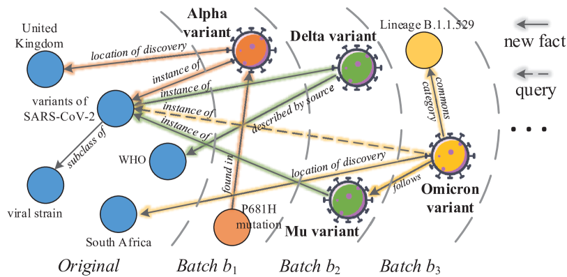
Figure 1. An illustration of how new entities emerge in real life, excerpted from Wikidata (Vrandečić and Krötzsch, 2014). Solid glowing links are new facts as new entities emerge, while dashed glowing links are queries, e.g., (Omicron variant, instance of, ?), to be inferred in the inductive KG reasoning task.

However, conventional KG reasoning models, e.g., (Bordes et al., 2013; Wang et al., 2014; Yang et al., 2015; Dettmers et al., 2018; Vashishth et al., 2020a; Chao et al., 2021; Yu et al., 2021; Vashishth et al., 2020b), are based on the closed-world assumption, where all entities must be seen during training. When new entities emerge, conventional models are unable to learn the embeddings for them unless re-training the whole KG from scratch. Although there have been some studies (Hamaguchi et al., 2017; Bhowmik and de Melo, 2020; Teru et al., 2020; Liu et al., 2021) to fill this deficiency, three critical defects of them in the settings put their actual reasoning ability into questions. First, existing work simulates only one single batch of emerging entities, which oversimplifies the real-world scenario where new entities are popping up continually. A real-world case extracted from Wikidata is illustrated in Fig. 1, which depicts how new virus variants continually emerge. Second, newly emerging entities usually have sparse links (Baek et al., 2020). We observe in many existing benchmark datasets (Hamaguchi et al., 2017; Wang et al., 2019) that the average degree of emerging entities is even higher than that of entities in the original KG. See Table 1 for example. Third, some existing studies (Hamaguchi et al., 2017; Wang et al., 2019) do not consider emerging facts between emerging entities, e.g., the fact (P681H mutation, found in, Alpha variant) in Fig. 1, where both “P681H mutation” and “Alpha variant” newly appear in batch $b_{1}$.

Table 1. Comparison between the average degree of original entities in the KG and that of new entities over all emerging batch(es). The left four datasets are taken from two existing works, MEAN (Hamaguchi et al., 2017) and LAN (Wang et al., 2019), as examples, whereas the right three datasets are constructed in this work.

Avg. degree	MEAN		LAN		Our MBE datasets
	H-1000	T-1000	Sub-10	Obj-10	WN	FB	NELL
$\mathcal{E}_{\text{Original}}$	5.7	5.3	21.1	18.8	3.7	34.9	5.3
$\mathcal{E}_{\text{New}}$	9.5	11.8	63.1	72.2	2.0	14.4	1.2

Towards a more realistic modeling of emerging entities, we provide a re-definition of emerging entities and the inductive KG reasoning task in a multi-batch emergence (MBE) scenario. Unlike previous work, in this scenario new entities emerge in chronological multiple batches, and their degrees are restrained to make sure that they have relatively few links. Under this MBE scenario with fewer auxiliary facts for new entities, inductive KG reasoning becomes much more challenging.

In this paper, we formulate the KG reasoning problem as reinforcement learning, and propose a new walk-based inductive model. We aim to resolve three key challenges:

1. How to transfer knowledge to the emerging batches?
   Inductive learning aims at transferring knowledge learned from seen data to unseen data. To better exploit transferable knowledge, a walk-based agent is used to conduct the reasoning process in our model. It can learn to explicitly leverage the neighboring information, which is transferable to new entities. (Section 3.2)

2. How to encode new entities without re-training?
   We design ARGCN, a graph convolutional network (GCN) with adaptive relation aggregation, to not only encode new entities as they come, but also update the embeddings of existing entities that are affected by the new entities. (Section 3.3) To attentively encode for specific queries, we devise a feedback attention mechanism which leverages logic rules extracted from reasoning trajectories to capture the varying neighbor importance of entities. (Section 3.4)

3. How to resolve the link sparsity of new entities?
   Oftentimes, emerging entities only have a few links, which limits the walk-based reasoning. To alleviate this problem, we introduce a link augmentation strategy to add trustworthy facts into KGs for providing more clues. (Section 3.5)

Because there is no off-the-shelf dataset for the MBE scenario, we develop three new datasets in this work. The new entities in our datasets are divided into multiple batches and contain relatively sparse neighbors. Furthermore, our datasets contain not only emerging facts that link new entities with existing entities (a.k.a. unseen-seen facts), but also emerging facts that connect two new entities (a.k.a. unseen-unseen facts). (Section 4)

We carry out extensive experiments on the new MBE datasets to compare with existing inductive models. The experimental results show that our model achieves the best reasoning performance on the inductive KG reasoning task. (Section 5)

In summary, the key contributions of this paper are threefold:

• To the best of our knowledge, we are the first to explore inductive KG reasoning under the MBE scenario, which is more realistic and challenging.

• We analyze the defects of the datasets in existing work, and construct new multi-batch datasets simulating real-world ever-growing KGs.

• We propose a walk-based inductive KG reasoning model to cope with this new scenario. Our experimental results demonstrate the superiority of the proposed model against various kinds of state-of-the-art inductive models.

2. Related Work

In this section, we review existing embedding-based, walk-based and rule-based inductive KG reasoning models.

2.1. Embedding-based Inductive KG Reasoning

Conventional embedding-based KG reasoning models (Bordes et al., 2013; Yang et al., 2015; Dettmers et al., 2018; Guo et al., 2019) rest on static KGs. As aforementioned, these models are unable to handle emerging entities. As far as we know, MEAN (Hamaguchi et al., 2017) is the first inductive work that can learn the embeddings of emerging entities without re-training. It simply aggregated the transitioned neighboring information and took the mean results as the embeddings of entities. Based on MEAN, LAN (Wang et al., 2019) incorporated the rule-based and neural attentions to measure the varying importance of different neighbors during aggregation. Both MEAN and LAN used a triple scoring function to rank each candidate fact. A limitation of them is that they can only deal with unseen-seen facts due to their dependence on existing entities for aggregation. GraIL (Teru et al., 2020) and TACT (Chen et al., 2021) scored an extracted subgraph between two entities of each candidate fact. They learned the entity-independent relational semantic patterns with graph neural networks (GNNs) to predict the missing relation for the entity pair. INDIGO (Liu et al., 2021) further exploited the structure information of KGs by fully encoding the annotated graphs which initialize entity features using their neighboring relation and node type information.

Other embedding-based work addressed specific settings or tasks of inductive KG reasoning. GEN (Baek et al., 2020) and HRFN (Zhang et al., 2021) explored the meta-learning setting where the edge degrees of entities are less than a small number. PathCon (Wang et al., 2021) encoded each entity pair via aggregating its neighboring edges, which is similar to our ARGCN. Note that the query setting of PathCon is relation prediction in the form of $(h,?,t)$, rather than the harder entity prediction studied in this paper. Since the settings and tasks of these studies cannot be directly adapted to the reasoning task under the MBE scenario, we do not discuss them in the rest of this paper.

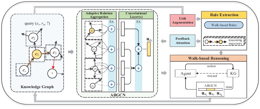
Figure 2. Our model consists of four modules: walk-based agent, ARGCN, feedback attention and link augmentation. Given a query $(e_{s},r_{q},?)$, we first use link augmentation to add trustworthy facts (e.g., the dotted red link from $e_{3}$ to $?$) into the KG. Then, we use ARGCN with feedback attention to attentively encode entities and relations. Based on the embeddings, the walk-based agent conducts reasoning in the KG. Particularly, during training, our model extracts the walk-based rules from the reasoning trajectories to support feedback attention and link augmentation.

2.2. Walk-based Inductive KG Reasoning

Instead of scoring candidate facts based on entity and relation embeddings, the KG reasoning problem can also be formulated in a reinforcement learning fashion, where a walk-based agent explores the reasoning paths to reach the target entities. DeepPath (Xiong et al., 2017) designed a KG-specific reinforcement learning environment and predicted the missing relations between entity pairs. MINERVA (Das et al., 2018) encoded the path history of an agent in a policy network and answered the missing tail entity of each query. Multi-Hop (Lin et al., 2018) advanced MINERVA by introducing reward reshaping and action dropout to enrich the reward signals and improve generalization. Other studies (Lv et al., 2019; Wan et al., 2020; Wan and Du, 2021) proposed more complex reward functions, policy networks or reinforcement learning frameworks. Particularly, GT (Bhowmik and de Melo, 2020) incorporated a graph Transformer for the walk-based reasoning and found that the walk-based models such as Multi-Hop can adapt well to the inductive setting, despite the emerging entities being randomly initialized. RuleGuider (Lei et al., 2020) leveraged the pre-mined high-quality rules generated from AnyBURL (Meilicke et al., 2019) to provide more reward supervision. Both RuleGuider and our model leverage the rules to provide more knowledge for reasoning. However, unlike RuleGuider, we do not need an extra rule mining model to obtain rules.

2.3. Rule-based Inductive KG Reasoning

Rule-based inductive models mine rules from KGs to help the prediction of missing facts. Early rule mining models, e.g., AMIE (Galárraga et al., 2013) and AMIE+ (Galárraga et al., 2015), aimed at accelerating the mining process using parallelization and partitioning. They used specific confidence measures to discover the rules of high quality. NeurLP (Yang et al., 2017) and DRUM (Sadeghian et al., 2019) learned the rules in an end-to-end differentiable manner, which computed a score for each fact and learned the rules by maximizing all fact scores. AnyBURL (Meilicke et al., 2019) extended the definition of rules to utilize more context information and devised a bottom-up method for efficient rule learning. The training process of walking-based models can also be regarded as rule mining, but their rules are implicit in the policy networks, rather than explicit in the form of Horn clauses. In this paper, we extract explicit rules from the walk-based trajectories to assist reasoning over growing KGs.

3. Proposed Model

In this section, we first introduce background concepts. Then, we present four key modules in our model, namely walk-based reasoning, ARGCN, feedback attention and link augmentation. The overview of our model is shown in Fig. 2.

3.1. Preliminaries

Expanding KG. In the MBE scenario, an expanding KG includes an existing KG called original and $N$ batches of emerging entities with concomitant facts:

• Original. Let $\mathcal{K}_{o}=\{(e_{h},r,e_{t})\,|\,e_{h}\in\mathcal{E}_{o},r\in\mathcal{R},e_{t}\in\mathcal{E}_{o}\}$ be the existing KG. $\mathcal{E}_{o}$, $\mathcal{R}$ are the entity and relation sets of $\mathcal{K}_{o}$, respectively. $(e_{h},r,e_{t})$ is called a fact, where $e_{h},r$ and $e_{t}$ are the head entity, relation and tail entity, respectively.

• Batches. The $i$-th ($0\leq i\leq N$) emerging batch is denoted by $\mathcal{K}_{i}=\{(e_{h},r,e_{t})\,|\,r\in\mathcal{R},e_{h}\in\mathcal{E}_{i}\lor e_{t}\in\mathcal{E}_{i}\}$, where $\mathcal{E}_{i}$ is the set of emerging entities appearing in this batch. $e_{h}$ and $e_{t}$ can both be emerging entities. Particularly, $\mathcal{K}_{0}=\mathcal{K}_{o}$. Note that we do not consider emerging relations in this paper.

Inductive KG reasoning aims to predict missing links for emerging entities. In this paper, each inductive KG reasoning query $q$ is a triple of $(e_{s},r_{q},?)$, where $?$ denotes the target entity to be inferred. At least one of $e_{s}$ and $?$ in $q$ is an emerging entity.

Walk-based reasoning is a process that an agent starts from a head entity, continuously takes actions to move, and reaches a final entity. For an $r_{q}$-specific query $(e_{s},r_{q},?)$, a reasoning trajectory is defined as a sequence of facts $(e_{s},r_{1},e_{1})\rightarrow(e_{1},r_{2},e_{2})\rightarrow\cdots\rightarrow(e_{n-1},r_{n},e_{\text{final}})$. We can extract a relation chain $r_{1}\rightarrow r_{2}\rightarrow\cdots\rightarrow r_{n}$ from the trajectory as a walk-based rule, denoted by $p$ for this $r_{q}$-specific query, i.e., $p:r_{q}\Leftarrow r_{1}\wedge r_{2}\wedge\ldots\wedge r_{n}$. If the final entity $e_{\text{final}}$ is the target entity, this trajectory is called a positive trajectory, otherwise it is called a negative trajectory. We record the numbers of positive and negative trajectories that each $p$ resides in as $\text{pos}(p)$ and $\text{neg}(p)$, respectively. We denote the set of walk-based rules by $\mathcal{M}$ and the rule set for the $r_{q}$-specific query by $\mathcal{M}_{r_{q}}$.

3.2. Walk-based Reasoning

We design a walk-based model to carry out the reasoning process.

Environment setting. We formulate the inductive KG reasoning as a Markov decision process (MDP) (Lin et al., 2018) and train a reinforcement learning agent to perform the walk-based reasoning on the KG. A typical MDP is a quadruple $(\mathcal{S},\mathcal{A},\delta,\mathcal{B})$. In this paper, each element is defined as follows:

• States. We define each state $s_{t}=\big{(}(e_{s},r_{q}),e_{t}\big{)}$ by combining the known part of query $(e_{s},r_{q},?)$ and entity $e_{t}$ where the agent locates at step $t$. $\mathcal{S}$ is the set of all possible states.

• Actions. In state $s_{t}$, the possible action space $\mathcal{A}_{t}=\big{\{}(r,e^{\prime})\,|\,$ $(e_{t},r,e^{\prime})\in\mathcal{K}_{o}\big{\}}\cup\big{\{}(r^{-},e^{\prime})\,|\,(e^{\prime},r^{-},e_{t})\in\mathcal{K}_{o}\big{\}}\cup\big{\{}(r_{\text{sl}},e_{t})\big{\}}$ is the union of neighboring edges of $e_{t}$ and a self-loop edge. $r^{-}$ denotes the reverse relation of $r$. The self-loop edge of an entity enables the agent to stay in the current state.

• Transitions. The transition function $\delta:\mathcal{S}\times\mathcal{A}\rightarrow\mathcal{S}$ defines the transitions among states. Following an action $a_{t}\in\mathcal{A}_{t}$, the agent moves from $s_{t}$ to the next state $s_{t+1}$.

• Rewards. After reaching the maximum number of moves, the agent stops on a final entity $e_{l}$ in state $s_{l}$. At that moment, a reward $\mathcal{B}$ is given to the agent, which is

  (1) $$\mathcal{B}(s_{l}\,|\,e_{s},r_{q})=\begin{cases}1,&\mbox{if }(e_{s},r_{q},e_{l})\in\mathcal{K}_{o}\\ 0,&\mbox{otherwise}\end{cases}.$$

Policy network. To solve the MDP problem, the agent needs a policy to determine which action to take in each state. We apply a neural network to parameterize the policy. In our policy network, the input consists of three parts: the embedding of $e_{t}$, the embedding of $r_{q}$ and the encoding of path history $(e_{s},r_{1},e_{1},\ldots,r_{t},e_{t})$. Here, we encode the path history with an LSTM as follows:

(2) $$\mathbf{h}_{0} =\mathrm{LSTM}\big{(}\mathbf{0},[\mathbf{u}_{r_{0}};\mathbf{u}_{e_{s}}]\big{)},$$

(3) $$\mathbf{h}_{t} =\mathrm{LSTM}\big{(}\mathbf{h}_{t-1},[\mathbf{u}_{r_{t}};\mathbf{u}_{e_{t}}]\big{)},\quad t>0,$$

where $\mathbf{u}_{r_{0}}\in\mathbb{R}^{d}$ is the embedding of a special starting relation $r_{0}$, and $\mathbf{h}_{t}\in\mathbb{R}^{2d}$ is the encoding of the path history. Then, the policy network is defined as

(4) $$\pi_{\theta}(a_{t}\,|\,s_{t})=\sigma\Big{(}\mathbf{A}_{t}\times\mathbf{W}_{\mathrm{fc2}}\mathrm{ReLU}\big{(}\mathbf{W}_{\mathrm{fc1}}[\mathbf{u}_{e_{t}};\mathbf{u}_{r_{q}};\mathbf{h}_{t}]\big{)}\Big{)},$$

where $\mathbf{A}_{t}\in\mathbb{R}^{|\mathcal{A}_{t}|\times 2d}$ is the stacked embeddings of all actions. $\sigma()$ is the softmax operator. $\mathbf{W}_{\mathrm{fc1}}\in\mathbb{R}^{2d\times 4d}$ and $\mathbf{W}_{\mathrm{fc2}}\in\mathbb{R}^{2d\times 2d}$ are the learnable weight matrices of two fully-connected layers.

Optimization. The objective of the policy network is to maximize the expected reward of all training queries:

(5) $$J(\theta)=\mathbb{E}_{(e_{s},r_{q},e_{o})\in\mathcal{K}_{o}}\Big{[}\mathbb{E}_{a_{1},\ldots,a_{l}\sim\pi_{\theta}}\big{[}\mathcal{B}(s_{l}\,|\,e_{s},r_{q})\big{]}\Big{]},$$

where $a_{l},s_{l}$ are the action and state of the last step, respectively.

We use the REINFORCE optimization algorithm (Williams, 1992) to train our model, and the stochastic gradient is formulated as

(6) $$\nabla_{\theta}J(\theta)\approx\nabla_{\theta}\sum_{t}\mathcal{B}(s_{l}\,|\,e_{s},r)\log\pi_{\theta}(a_{t}\,|\,s_{t}).$$

It is worth noting that the embeddings of entities are also parameters to be learned. So, when new entities are added into the KG, the trained model cannot properly handle them since they do not have trained embeddings yet.

3.3. ARGCN

As just mentioned, the walk-based agent cannot encode emerging entities properly. To solve this problem, we propose a GCN with adaptive relation aggregation (ARGCN) as our encoder. Specifically, we first adopt an adaptive relation aggregation layer to aggregate the information of linked relations for each entity, and then use the stacked convolutional layers proposed in CompGCN (Vashishth et al., 2020b) to aggregate the information of multi-hop neighbors.

Adaptive relation aggregation layer. Different from existing relational GNNs (Schlichtkrull et al., 2018; Vashishth et al., 2020b) which randomly initialize the base embedding of each entity for training, we introduce an adaptive relation aggregation layer to learn the base embedding of each entity by solely aggregating its linked relations.

For an entity $e$ in $\mathcal{K}_{o}$, we generate its base embedding $\mathbf{u}_{e}^{b}\in\mathbb{R}^{d}$ as follows:

(7) $$\mathbf{u}_{e}^{b}=\tanh\Big{(}\sum_{(r,e^{\prime})\in\mathcal{N}_{\mathrm{in}}(e)}\mathbf{W}_{\mathrm{in}}\mathbf{z}_{r}+\sum_{(r,e^{\prime})\in\mathcal{N}_{\mathrm{out}}(e)}\mathbf{W}_{\mathrm{out}}\mathbf{z}_{r}\Big{)},$$

where $\mathcal{N}_{\mathrm{in}}(e)=\big{\{}(r,e^{\prime})\,|\,(e^{\prime},r,e)\in\mathcal{K}_{o}\big{\}},\mathcal{N}_{\mathrm{out}}(e)=\big{\{}(r,e^{\prime})\,|\,(e,r,$ $e^{\prime})\in\mathcal{K}_{o}\big{\}}$. $\mathbf{W}_{\mathrm{in}},\mathbf{W}_{\mathrm{out}}\in\mathbb{R}^{d\times d}$ are two learnable weight matrices. $\mathbf{z}_{r}\in\mathbb{R}^{d}$ is the learnable embedding of relation $r$ initialized with the Xavier normal initialization. $\tanh()$ is employed as the activation function.

Stacked convolutional layers. We use a stacked multi-layered GCN to aggregate the multi-level neighboring information. The entity and relation embeddings are updated as follows:

(8) $$\begin{split}\mathbf{u}^{l+1}_{e}&=\tanh\Big{(}\mathbf{W}^{l}_{\mathrm{self}}\mathbf{u}_{e}^{l}+\sum_{(r,e^{\prime})\in\mathcal{N}_{\mathrm{in}}(e)}\mathbf{W}_{\mathrm{in}}^{l}\phi\big{(}\mathbf{u}_{e^{\prime}}^{l},\mathbf{u}^{l}_{r}\big{)}\\ &\qquad\qquad\qquad\quad+\sum_{(r,e^{\prime})\in\mathcal{N}_{\mathrm{out}}(e)}\mathbf{W}_{\mathrm{out}}^{l}\phi\big{(}\mathbf{u}_{e^{\prime}}^{l},\mathbf{u}^{l}_{r}\big{)}\Big{)},\end{split}$$

(9) $$\mathbf{u}_{r}^{l+1} =\mathbf{W}_{\mathrm{rel}}^{l}\mathbf{u}_{r}^{l},$$

where $\mathbf{u}^{0}_{e}=\mathbf{u}^{b}_{e},\mathbf{u}^{0}_{e^{\prime}}=\mathbf{u}^{b}_{e^{\prime}},\mathbf{u}^{0}_{r}=\mathbf{z}_{r}$. $\mathbf{W}^{l}_{\mathrm{in}},\mathbf{W}^{l}_{\mathrm{out}},\mathbf{W}^{l}_{\mathrm{self}}\in\mathbb{R}^{d\times d}$ are three learnable weight matrices for entity embedding update, and $\mathbf{W}^{l}_{\mathrm{rel}}\in\mathbb{R}^{d\times d}$ is a learnable weight matrix for relation embedding update. The transition function $\phi:\mathbb{R}^{d}\times\mathbb{R}^{d}\to\mathbb{R}^{d}$ receives relation-entity pairs as input and aggregates the messages from neighboring links. We use the element-wise product for $\phi(\mathbf{u}_{e^{\prime}},\mathbf{u}_{r})=\mathbf{u}_{e^{\prime}}\circ\mathbf{u}_{r}$.

3.4. Feedback Attention

Transferring knowledge from seen data to unseen data is crucial for inductive reasoning. To transfer the KG reasoning patterns to emerging batches, we introduce a feedback attention mechanism which leverages the walk-based rules to capture the importance of neighboring relations for ARGCN.

First, we calculate the confidence value of each walk-based rule $p$ as follows:

(10) $$\text{conf}(p)=\frac{\text{pos}(p)}{\text{pos}(p)+\text{neg}(p)}.$$

Then, for $r_{q}$-specific queries, we calculate the correlation between $r_{q}$ and each other relation $r_{j}$ in the KG. We collect the walk-based rules containing $r_{j}$, and take the maximum confidence value of these rules as the correlation between $r_{q}$ and $r_{j}$:

(11) $$\text{corr}(r_{q},r_{j})=\max\big{\{}\text{conf}(p_{i})\,|\,p_{i}\in\mathcal{M}_{r_{q}}\wedge r_{j}\in p_{i}\big{\}}.$$

If $r_{j}$ is not in any walk-based rules, the correlation is set to 0.

At last, the weight of each $r_{j}$ given the query relation $r_{q}$ is

(12) $$\alpha_{r_{j}\,|\,r_{q}}=\lambda_{r_{q}}\,\text{corr}(r_{q},r_{j})+(1-\lambda_{r_{q}}),$$

where $\lambda_{r_{q}}=\tanh\big{(}\frac{1}{\epsilon}\sum_{p_{i}\in\mathcal{M}_{r_{q}}}\text{pos}(p_{i})\big{)}\in(0,1)$ and $\epsilon$ is a fixed hyperparameter. Here we leverage $\lambda_{r_{q}}$ as a reliability measure to adjust the attention because the confidence of walk-based rules may not be reliable in the first few training iterations due to the small number of reasoning trajectories.

Put it all together, the re-formulated Eqs. (7) and (8) after incorporating the feedback attentions are

(13) $$\begin{split}\mathbf{u}_{e}^{b}&=\tanh\Big{(}\sum_{(r,e^{\prime})\in\mathcal{N}_{\mathrm{in}}(e)}\alpha_{r\,|\,r_{q}}\mathbf{W}_{\mathrm{in}}\mathbf{z}_{r}\\ &\qquad\qquad\qquad\quad+\sum_{(r,e^{\prime})\in\mathcal{N}_{\mathrm{out}}(e)}\alpha_{r\,|\,r_{q}}\mathbf{W}_{\mathrm{out}}\mathbf{z}_{r}\Big{)},\end{split}$$

(14) $$\begin{split}\mathbf{u}^{l+1}_{e}&=\tanh\Big{(}\mathbf{W}_{\mathrm{self}}\mathbf{u}_{e}^{l}+\sum_{(r,e^{\prime})\in\mathcal{N}_{\mathrm{in}}(e)}\alpha_{r\,|\,r_{q}}\mathbf{W}_{\mathrm{in}}^{l}\phi\big{(}\mathbf{u}_{e^{\prime}}^{l},\mathbf{u}^{l}_{r}\big{)}\\ &\qquad\qquad\qquad\quad+\sum_{(r,e^{\prime})\in\mathcal{N}_{\mathrm{out}}(e)}\alpha_{r\,|\,r_{q}}\mathbf{W}_{\mathrm{out}}^{l}\phi\big{(}\mathbf{u}_{e^{\prime}}^{l},\mathbf{u}^{l}_{r}\big{)}\Big{)}.\end{split}$$

We take the output of the last layer as the final embeddings and use them in the walk-based reasoning process. With new entities and facts emerging, ARGCN adaptively aggregates relations in the new KG to generate and update the embeddings.

3.5. Link Augmentation

KGs are widely acknowledged as incomplete (Wang et al., 2017; Ji et al., 2021; Rossi et al., 2021). Especially, emerging entities often suffer from the sparse link problem. Many links of emerging entities have not been added to the KG, which hinders the reasoning on them. For example, as shown in Fig. 2, due to the sparse links between the start entity $e_{s}$ and the target entity ?, the walk-based agent can hardly answer this query. However, if we can complement the missing link between $e_{3}$ and ?, this query would be likely to be answered. Motivated by this, we propose a link augmentation strategy to add trustworthy facts into the KG for providing more reasoning clues.

Specifically, the link augmentation consists of two stages: generate candidate links and identify trustworthy ones. For candidate link generation, there are two methods: one is combining each entity in $\mathcal{E}$ and each relation in $\mathcal{R}$ one by one; the other is only combining the head entities that exist in the current facts $\mathcal{K}$ and their relations. The time complexity of the first method is $O(|\mathcal{E}|\times|\mathcal{R}|)$, which is very time-consuming. In practice, we find that this would also introduce a lot of noises, since there are no negative samples in the walk-based learning process. So, we apply the second method, which only has a time complexity of $O(|\mathcal{K}|)$.

To identify the trustworthy ones from candidate links, we leverage the walk-based rules as prior knowledge to select the trustworthy tail entities. Inspired by the traditional rule-based models (Galárraga et al., 2013, 2015), we use two metrics, confidence and support, to measure the trustworthiness of rules, and use it to identify trustworthy rules:

(15) $$\mathcal{P}=\big{\{}p\in\mathcal{M}\,|\,\text{conf}(p)\geq\gamma_{1}\wedge\text{pos}(p)\geq\gamma_{2}\big{\}}.$$

where $\mathcal{P}$ is the set of trustworthy rules, $\gamma_{1}$ is the confidence threshold, and $\gamma_{2}$ is the support threshold.

Then, we use the rules in $\mathcal{P}$ to select trustworthy facts. Specifically, for each candidate $(e_{s},r_{q})$, we use the $r_{q}$-specific rules to select tail entities to constitute the trustworthy facts. The generated fact set $\mathcal{L}$ can be formulated as

$$\mathcal{L} =\Big{\{}(e_{s},r_{q},e_{t})\,|\,\exists\big{\{}(e_{s},r_{1},e_{1}),(e_{1},r_{2},e_{2}),\ldots,(e_{n},r_{n},e_{t})\big{\}}\in\mathcal{K}$$

(16) $$\qquad\qquad\wedge(r_{1}\rightarrow r_{2}\rightarrow\cdots\rightarrow r_{n})\in\mathcal{P}_{r_{q}}\wedge r_{q}\in\mathcal{R}\Big{\}},$$

where $\mathcal{P}_{r_{q}}$ is a set of $r_{q}$-specific rules and $\mathcal{P}_{r_{q}}\subseteq\mathcal{P}$.

Finally, we add $\mathcal{L}$ into the KG at the start of reasoning. Note that some trustworthy facts are duplicates of facts in the KG, but we still add them into the KG as the special rule-based facts. When an original fact is masked in the training stage, the agent may directly walk to the target entity through a duplicate rule-based fact. With new entities and facts emerging, the link augmentation also generates trustworthy facts for new queries.

Input: Training set $\mathcal{T}$ of the original KG $\mathcal{K}_{o}$.

Output: Model parameters $\theta$ and walk-based rule set $\mathcal{M}$.

1 Initialize $\theta;\mathcal{M}\leftarrow\emptyset$, and augmentation fact set $\mathcal{L}\leftarrow\emptyset$;

2 for $epoch$ $\leftarrow 1$ to $max\_epochs$ do

3       Update $\mathcal{L}$ and feedback attentions based on $\mathcal{M}$;

4       Update the embeddings based on ARGCN with feedback attentions;

5       foreach query $(e_{s},r_{q})$ in $\mathcal{T}$ do

6             for $step\leftarrow 1$ to $max\_steps$ do

7                   The agent selects an action from $\mathcal{T}\cup\mathcal{L}$;

8                   The agent walks to the next entity;

9                  

10            Calculate the loss using Eq. (1);

11             Update $\theta$ using Eq. (5);

12             Update $\mathcal{M}$ based on the generated reasoning trajectories;

13            

14      

Algorithm 1 Training process

Table 2. Statistics of the three constructed MBE datasets. $\mathcal{T},\mathcal{V},\mathcal{E}_{o},\mathcal{R}$ denote the sets of training facts, validation facts, entities and relations in the original KG, respectively. $\mathcal{S}_{i},\mathcal{Q}_{i},\mathcal{E}_{i}$ ($1\leq i\leq 5$) are the sets of emerging facts, query facts and new entities of the $i$-th batch, respectively.

Datasets	Original				Batch $b_{1}$			Batch $b_{2}$			Batch $b_{3}$			Batch $b_{4}$			Batch $b_{5}$
	$|\mathcal{T}|$	$|\mathcal{V}|$	$|\mathcal{E}_{o}|$	$|\mathcal{R}|$	$|\mathcal{S}_{1}|$	$|\mathcal{Q}_{1}|$	$|\mathcal{E}_{1}|$	$|\mathcal{S}_{2}|$	$|\mathcal{Q}_{2}|$	$|\mathcal{E}_{2}|$	$|\mathcal{S}_{3}|$	$|\mathcal{Q}_{3}|$	$|\mathcal{E}_{3}|$	$|\mathcal{S}_{4}|$	$|\mathcal{Q}_{4}|$	$|\mathcal{E}_{4}|$	$|\mathcal{S}_{5}|$	$|\mathcal{Q}_{5}|$	$|\mathcal{E}_{5}|$
WN-MBE	35,426	8,858	19,361	11	5,678	1,352	3,723	6,730	1,874	4,122	7,545	2,054	4,300	8,623	2,493	4,467	9,608	2,762	4,514
FB-MBE	125,769	31,442	7,203	237	18,394	9,240	1,458	19,120	9,669	1,461	19,740	9,887	1,467	22,455	11,127	1,467	22,214	11,059	1,471
NELL-MBE	88,814	22,203	33,348	200	4,496	853	4,488	5,411	1,059	6,031	6,543	1,277	7,660	7,667	1,427	9,056	8,876	1,595	10,616

3.6. Training and Answering Pipeline

We integrate the above modules together and present a pipeline of training process in Algorithm 1. We are given a set of facts as the training data. After initialization, for each training epoch, we first update the augmentation fact set and feedback attentions based on the rule set $\mathcal{M}$. Then, we update entity embeddings using ARGCN with feedback attention in Line 4. In Lines 6–10, we perform the walk-based reasoning and calculate the loss to update the parameters $\theta$ of our model. In Line 11, we update the rule set $\mathcal{M}$ using the generated reasoning trajectory. Finally, the output is the learned model parameters and the set of walk-based rules.

With new entities and facts coming, we freeze parameters and perform query answering on the new KG, in the same way as Lines 6–8 in Algorithm 1.

4. Datasets

To conduct a realistic evaluation for inductive KG reasoning, we construct three MBE datasets based on WN18RR (Dettmers et al., 2018), FB15K-237 (Toutanova and Chen, 2015) and NELL-995 (Xiong et al., 2017), and name them as WN-MBE, FB-MBE and NELL-MBE, respectively. Here, we describe the steps to construct our MBE datasets. Given a static KG $\mathcal{G}$ (e.g., NELL), we generate a MBE dataset consisting of an original KG $\mathcal{K}_{o}$ and five emerging batches. $\mathcal{K}_{o}$ contains a training set $\mathcal{T}$ and a validation set $\mathcal{V}$. Each emerging batch $b_{i}$ contains an emerging fact set $\mathcal{S}_{i}$ and a query set $\mathcal{Q}_{i}$. The construction steps are as follows:

• Seeding. We randomly sample $n$ entities in $\mathcal{G}$ as the seeds, and use them to constitute $\mathcal{E}_{o}$.

• Growing. We treat the seed entities in $\mathcal{E}_{o}$ as root nodes and conduct the breadth-first-search in $\mathcal{G}$. During the traversal, we add each visited entity into $\mathcal{E}_{o}$ with a probability $p$. This step is repeated until $|\mathcal{E}_{o}|\geq\frac{|\mathcal{E}_{\mathcal{G}}|}{2}$. Then, the entities not in $\mathcal{E}_{o}$ form another set $\mathcal{E}_{n}$.

• Dividing. For each fact in $\mathcal{G}$, we add it into $\mathcal{K}_{o}$ if both of its entities are in $\mathcal{E}_{o}$. We divide $\mathcal{K}_{o}$ into a training set $\mathcal{T}$ and a validation set $\mathcal{V}$ by a ratio $4:1$ on fact size. $\mathcal{E}_{n}$ is evenly divided into five batches, which simulates the MBE scenario. Then, for each batch, its corresponding emerging facts are chosen out from $\mathcal{G}$. Next, these facts are divided into an emerging fact set $\mathcal{S}_{i}$ and a query set $\mathcal{Q}_{i}$ using the minimal-spanning tree algorithm. The facts appearing in the trees are classified into $\mathcal{S}_{i}$ and the ones not in the trees constitute $\mathcal{Q}_{i}$. Using this algorithm avoids emerging entities to appear in the query sets only.

• Cleaning. Lastly, a few extra operations are done to ensure: (1) no new relations appear in the five batches; (2) for each batch, it should not contain any later emerging entity (i.e., chronological correctness); and (3) $\mathcal{E}_{\mathcal{V}}\subseteq\mathcal{E}_{\mathcal{T}}$, $\mathcal{E}_{\mathcal{O}_{i}}\subseteq\mathcal{E}_{\mathcal{T}}$ $\cup\,\mathcal{E}_{\mathcal{S}_{1}}\cup\ldots\cup\mathcal{E}_{\mathcal{S}_{i}}$. Note that these operations may cause some isolated new entities, which are discarded.

In implementation, we set $n=5,000,p=0.5$; $n=4,000,p=0.5$ and $n=3,000,p=0.6$ for constructing WN-MBE, FB-MBE and NELL-MBE, respectively. The construction steps can easily repeat to discretionary amounts of emerging batches.

Table 2 depicts the statistics of the three datasets. Our datasets satisfy the characteristic that new entities have sparse links (see Table 1 in Section 1).

5. Experiments and Results

In this section, we assess the proposed model and report our experimental results. The source code and constructed datasets are available at https://github.com/nju-websoft/MBE.

Table 3. Hits@1 results of tail entity prediction under 1 vs. all. The best Hits@1 scores in each batch are marked in bold.

Models	WN-MBE					FB-MBE					NELL-MBE
	$b_{1}$	$b_{2}$	$b_{3}$	$b_{4}$	$b_{5}$	$b_{1}$	$b_{2}$	$b_{3}$	$b_{4}$	$b_{5}$	$b_{1}$	$b_{2}$	$b_{3}$	$b_{4}$	$b_{5}$
MEAN	2.3	2.0	0.5	0.6	0.2	17.9	19.7	19.4	17.0	17.5	8.2	4.5	4.2	2.6	4.9
LAN	2.7	2.9	2.6	4.3	1.5	21.2	21.3	18.8	16.5	16.9	14.1	11.2	10.3	8.3	7.0
Multi-Hop	80.6	79.7	78.8	79.0	79.9	31.1	30.3	29.9	28.2	28.2	59.6	60.2	60.8	64.6	63.9
GT	82.0	82.4	82.9	81.8	81.1	31.7	31.2	30.6	29.2	29.9	61.5	61.0	60.9	64.3	64.2
RuleGuider	79.2	80.2	77.8	75.9	75.9	24.6	25.1	23.9	22.3	23.0	57.1	52.9	56.9	58.7	59.8
NeurLP	80.1	76.5	72.5	73.8	73.7	23.1	23.1	23.2	22.5	23.3	47.4	43.4	43.1	46.8	46.1
DRUM	81.9	79.0	75.6	76.4	76.7	24.0	24.2	24.4	24.0	25.1	47.5	43.2	43.3	47.2	46.6
AnyBURL	83.6	82.9	79.2	78.3	77.4	29.1	27.5	16.5	26.0	26.5	56.4	57.4	61.8	62.8	64.4
Ours	84.5	84.9	85.1	84.4	83.9	32.6	32.6	31.8	30.9	32.1	61.5	63.0	67.0	67.2	69.9

Table 4. MRR results of tail entity prediction under 1 vs. all. The best MRR scores in each batch are marked in bold.

Models	WN-MBE					FB-MBE					NELL-MBE
	$b_{1}$	$b_{2}$	$b_{3}$	$b_{4}$	$b_{5}$	$b_{1}$	$b_{2}$	$b_{3}$	$b_{4}$	$b_{5}$	$b_{1}$	$b_{2}$	$b_{3}$	$b_{4}$	$b_{5}$
MEAN	13.1	10.3	8.2	7.1	6.2	29.0	31.3	30.5	28.3	28.0	16.5	11.0	9.1	7.9	8.5
LAN	17.6	17.3	17.7	17.6	16.7	31.9	33.0	30.3	27.4	26.7	22.2	20.4	18.1	16.7	14.5
Multi-Hop	83.4	82.9	82.2	82.3	83.1	40.6	40.1	39.4	37.9	38.2	65.9	65.9	69.4	71.9	72.4
GT	83.9	85.1	84.9	84.2	84.6	41.6	40.3	39.7	39.1	39.2	66.0	67.0	70.6	71.8	72.6
RuleGuider	82.9	83.0	82.1	81.3	81.5	33.4	34.2	32.4	30.6	31.4	64.5	62.0	66.8	69.1	70.1
NeurLP	82.1	79.0	75.4	76.7	76.7	30.7	30.6	30.7	30.4	31.0	52.4	47.3	47.4	51.4	50.3
DRUM	80.1	76.6	72.9	73.3	74.0	31.6	31.4	31.7	31.5	32.5	53.1	47.7	47.7	51.6	50.6
AnyBURL	85.7	85.8	83.5	83.2	82.8	37.6	36.1	23.7	34.7	35.0	63.0	62.7	67.0	68.8	70.9
Ours	86.6	86.8	86.6	86.9	86.4	42.6	42.4	42.0	40.1	41.5	66.2	67.2	71.9	72.7	75.4

5.1. Experiment Settings

Competitors. We compare our model with ten inductive KG reasoning models, including four embedding-based models: MEAN (Hamaguchi et al., 2017), LAN (Wang et al., 2019) GraIL (Teru et al., 2020) and INDIGO (Liu et al., 2021)); three walk-based models: Multi-Hop (Lin et al., 2018), GT (Bhowmik and de Melo, 2020) and RuleGuider (Lei et al., 2020); and three rule-based models: NeurLP (Yang et al., 2017), DRUM (Sadeghian et al., 2019) and AnyBURL (Meilicke et al., 2019).

Implementation details. Since some comparative models are not originally designed for multi-batch emerging entities, we do some particular modifications to enable them. For the embedding-based models, after they generate embeddings for one batch, we combine them into $\mathcal{K}_{o}$ for the next batch. For the walk-based models, when testing queries in the $i$-th batch, we conduct reasoning on $\mathcal{K}_{o}\cup\mathcal{S}_{1}\cup\ldots\cup\mathcal{S}_{i}$. Note that Multi-Hop is not inherently inductive. Following (Bhowmik and de Melo, 2020), we use the Xavier normal initialization to assign a random vector to each emerging entity as its embedding. As for the rule-based models, they mine rules in $\mathcal{T}$. We use the official code to run all competing models. To run a model on the constructed datasets, we train it on $\mathcal{T}$ and validate it on $\mathcal{V}$. During testing, we freeze all parameters and only perform reasoning on $\mathcal{K}_{o}\cup\mathcal{S}_{1}\cup\ldots\cup\mathcal{S}_{i}$. In detail, we train 1,000 epochs for MEAN and LAN, 3,000 epochs for INDIGO, which are the same as those in their papers. We train 100 epochs for Multi-Hop, GT and our model. The model with the best validation performance is used for inductive reasoning on the test sets. All experiments are performed on a server with two NVIDIA RTX 3090 GPUs, two Intel Xeon Gold 5122 CPUs and 384GB RAM.

Parameter configuration. During training, we tune the hyperparameters of competing models and our model with grid search. For MEAN and LAN, the range of entity and relation embedding dimension is {50, 100}, the learning rate is {0.0005, 0.001, 0.01}, the training batch size is {512, 1,024}, the neighbor number is {15, 25, 35} for FB-MBE and {3, 5, 10} for WN-MBE and NELL-MBE. For INDIGO, the hidden vector dimension is set to 64, the range of learning rate is {0.0005, 0.001}, and the dropout rate is {0.2, 0.5}. For Multi-Hop, GT and RuleGuider, the dimension of relations and entities is set to 100, the range of learning rate is {0.001, 0.005, 0.001}, the beam size is set to 128, the number of LSTM (i.e., history encoder) layers is set to 3, the range of maximum walk steps is {3, 4, 5}, the action dropout rate is set to 0.1 for WN-MBE, 0.5 for FB-MBE, and 0.3 for NELL-MBE. For RuleGuider, the rule threshold is set to 0.15. For our model, the settings are the same as the above walk-based models except the range of GCN layer number is {1, 2, 3}, and $\epsilon$ is set to 1,000.

Evaluation metrics. Following the convention (Lin et al., 2018; Bhowmik and de Melo, 2020; Lei et al., 2020), we conduct the experiments on tail entity prediction. Two different comparison settings are considered. In the first setting (named “1 vs. all”), we compare with MEAN, LAN and all walk-based and rule-based competitors. These competitors, together with our model, calculate a score $f(e_{s},r_{q},e_{c})$ for each candidate entity $e_{c}$, where the total pool of candidates is all seen entities including emerging entities in previous batches. For the walk-based models, we set the scores of unreachable entities to $-\infty$. In the second setting (named “1 vs. 100”), we compare with GraIL and INDIGO. These two competitors need subgraph building and scoring to rank candidate entities for each test query, which are very time- and space-consuming. Thus, rather than using all seen entities as the candidate pool, we follow the setting of GraIL and INDIGO (Teru et al., 2020; Liu et al., 2021) and randomly choose 100 negative entities for each gold target entity in ranking. Moreover, because FB-MBE has denser links which cause the subgraph building and scoring process very slow (e.g., GraIL takes about 154 seconds to answer one query, while INDIGO takes about 22 seconds), we do not compare on FB-MBE but only perform the experiments on WN-MBE and NELL-MBE.

Again, following the convention, we pick two metrics of entity prediction: Hits@1 and mean reciprocal rank (MRR). We take the filtered mean ranks of gold target entities to calculate Hits@1 and MRR. Larger scores indicate better performance.

Table 5. Hits@1 results of tail entity prediction of GraIL, INDIGO and our model under 1 vs. 100. The best scores are marked in bold.

Models	WN-MBE					NELL-MBE
	$b_{1}$	$b_{2}$	$b_{3}$	$b_{4}$	$b_{5}$	$b_{1}$	$b_{2}$	$b_{3}$	$b_{4}$	$b_{5}$
GraIL	94.5	94.3	95.2	95.3	95.4	43.4	51.1	62.1	68.1	73.5
INDIGO	17.9	18.2	19.3	21.2	21.4	49.2	47.7	46.8	47.1	47.2
Ours	94.2	94.8	93.4	94.2	93.8	79.1	78.7	84.1	86.1	87.4

Table 6. MRR results of tail entity prediction of GraIL, INDIGO and our model under 1 vs. 100. The best scores are marked in bold.

Models	WN-MBE					NELL-MBE
	$b_{1}$	$b_{2}$	$b_{3}$	$b_{4}$	$b_{5}$	$b_{1}$	$b_{2}$	$b_{3}$	$b_{4}$	$b_{5}$
GraIL	95.7	95.8	96.4	96.5	96.5	56.8	63.3	72.3	77.6	81.3
INDIGO	30.7	31.1	31.5	33.7	34.2	62.6	60.5	59.5	59.9	60.0
Ours	95.2	95.3	93.8	94.5	94.2	79.8	79.5	84.7	86.6	87.6

5.2. Main Results

1 vs. all. The inductive KG reasoning results under this setting are presented in Tables 3 and 4. We observe that (1) our model outperforms all competitors on all emerging batches of the three datasets. (2) The embedding-based models MEAN and LAN have the worst Hits@1 and MRR results among all three types of competitors. Also, their performance on the sparse datasets WN-MBE and NELL-MBE is much worse compared to their performance on FB-MBE, which indicates the dependency of embedding-based models on dense links to well learn neighbor aggregators. (3) Among the walk-based models Multi-Hop, GT, RuleGuider and ours, Multi-Hop performs worse than GT and our model because it randomly initializes the embeddings of emerging entities and infers based solely on the query relations and neighboring links. GT leverages Transformer to handle emerging entities. It achieves the second-best performance, and is only inferior to ours. Although RuleGuider introduces more rewards into reinforcement learning than Multi-Hop, it performs worse. We believe that the deterioration is due to the two agent design of RuleGuider increases its dependence on well-learned entity embeddings, but RuleGuider can only randomly initialize new entity embeddings. (4) NeurLP, DRUM and AnyBURL are naturally adaptable to the inductive setting. But the rule-based models have poorer ability on exploring extensive potential paths and capturing complex structural patterns, which limits their inference performance especially on the dense dataset FB-MBE.

1 vs. 100. The Hits@1 and MRR results under this setting are shown in Tables 5 and 6. As mentioned in Section 5.1, GraIL uses a very time- and space-consuming testing process. It extracts and utilizes subgraphs between start entities and candidate tail entities, which capture more structural information to calculate scores. Even so, the results of GraIL are still worse than ours on NELL-MBE and only slightly better than ours on WN-MBE. From a high level, INDIGO and ARGCN in our model are similar in the way of dynamically generating base embeddings for entities. However, the performance of INDIGO is inferior to ours, especially on WN-MBE with only 11 relations. The reason for this is that the entity encoding dimension of INDIGO is fixed with the relation number, therefore it may not be trained sufficiently.

Table 7. Hits@1 results of ablation study.

Variants	WN-MBE					FB-MBE
	$b_{1}$	$b_{2}$	$b_{3}$	$b_{4}$	$b_{5}$	$b_{1}$	$b_{2}$	$b_{3}$	$b_{4}$	$b_{5}$
Base model	80.6	79.7	78.8	79.0	79.9	31.1	30.3	29.9	28.2	28.2
+ ARGCN	81.1	80.8	80.5	81.4	81.8	32.2	31.2	31.6	29.9	31.2
+ ARGCN & FA	82.2	81.3	81.1	81.6	82.2	32.5	31.9	32.5	30.2	31.4
+ LA	84.1	84.6	84.7	84.2	83.5	31.9	30.5	30.3	28.4	29.1
Intact model	84.5	84.9	85.1	84.4	83.9	32.6	32.6	31.8	30.9	32.1

Table 8. MRR results of ablation study.

Variants	WN-MBE					FB-MBE
	$b_{1}$	$b_{2}$	$b_{3}$	$b_{4}$	$b_{5}$	$b_{1}$	$b_{2}$	$b_{3}$	$b_{4}$	$b_{5}$
Base model	83.4	82.9	82.2	82.3	83.1	40.6	40.1	39.4	37.9	38.2
+ ARGCN	83.6	84.4	83.3	83.9	84.1	41.8	41.9	41.4	39.9	40.7
+ ARGCN & FA	84.0	84.4	83.7	84.1	84.8	41.9	42.1	41.9	40.1	41.0
+ LA	85.5	86.3	86.0	86.7	85.8	41.6	40.6	40.0	38.6	39.1
Intact model	86.6	86.8	86.6	86.9	86.4	42.6	42.4	42.0	40.1	41.5

Ablation study. To validate the effect of different modules in our model, we conduct an ablation study. Due to the space limitation, we only show the results on WN-MBE and FB-MBE in Tables 7 and 8. Similar conclusions can be observed on NELL-MBE. Specifically, we design four variants of our intact model: base model, “+ ARGCN”, “+ ARGCN & FA” (i.e., ARGCN with feedback attention), and “+ LA” (link augmentation). The base model is a vanilla multi-hop inductive model without any additional modules proposed in our model, and it is identical to the competitor Multi-Hop. The later three variants add specific module(s) into the base model. We observe that the three modules have different impacts on the sparse and dense datasets. (1) Compared with the base model, other three variants with additional modules all achieve better reasoning performance. (2) Compared to the base model, “+ ARGCN” variant stabilizes the performance as more batches come. This shows that ARGCN can effectively handle new entities. (3) “+ ARGCN & FA” outperforms “+ ARGCN”, which implies that the feedback attention module helps the aggregation layer focus more on important relations that are relevant to specific queries. (4) “+ LA” variant performs better than the base model especially on WN-MBE, which indicates the significance to conduct link augmentation for sparse KGs.

Table 9. Hits@1 results of replacing the walk-based rules with the pre-mined rules by AnyBURL on WN-MBE.

Models	$b_{1}$	$b_{2}$	$b_{3}$	$b_{4}$	$b_{5}$
Our model w/ AnyBURL	83.2	84.5	84.3	84.2	83.6
Our model w/ walk-based rules	84.5	84.9	85.1	84.4	83.9

Table 10. MRR results of replacing the walk-based rules with the pre-mined rules by AnyBURL on WN-MBE.

Models	$b_{1}$	$b_{2}$	$b_{3}$	$b_{4}$	$b_{5}$
Our model w/ AnyBURL	84.8	86.3	86.0	87.0	86.3
Our model w/ walk-based rules	86.4	87.2	87.4	87.3	86.9

5.3. Further Analyses

Table 11. Hits@1 and MRR results over unseen-seen and unseen-unseen queries. The last row denotes the proportion of unseen-unseen queries in the test set of each batch.

Metrics	Queries	WN-MBE					FB-MBE					NELL-MBE
		$b_{1}$	$b_{2}$	$b_{3}$	$b_{4}$	$b_{5}$	$b_{1}$	$b_{2}$	$b_{3}$	$b_{4}$	$b_{5}$	$b_{1}$	$b_{2}$	$b_{3}$	$b_{4}$	$b_{5}$
Hits@1	Unseen-seen	84.3	85.1	86.2	85.8	85.0	32.3	32.2	31.7	30.9	31.9	57.7	57.6	59.7	61.0	71.9
	Unseen-unseen	85.4	83.8	77.5	74.1	73.6	38.1	41.1	33.3	30.6	36.2	91.7	83.5	85.2	81.3	65.7
MRR	Unseen-seen	86.4	87.0	87.5	88.3	87.4	42.4	42.1	42.0	40.1	41.4	62.7	61.5	64.5	65.7	75.2
	Unseen-unseen	87.4	86.0	80.5	76.9	76.8	46.5	49.1	41.1	40.2	44.0	93.8	88.5	90.5	88.5	75.9
% of unseen-unseen		16.0	16.6	13.1	12.2	5.7	4.6	4.2	4.4	4.3	9.5	11.3	21.0	28.5	30.6	32.4

Incorporating pre-mined rules. In this analysis, we replace the walk-based rules with pre-mined rules. Specifically, we first use AnyBURL (Meilicke et al., 2019) as the rule miner to discover rules. Then, we use the found rules to generate feedback attentions and augmentation facts. Note that the pre-mined rules are not updated during training. Tables 9 and 10 show the results on WN-MBE. We see that our model can still gain satisfactory results, despite that the results are slightly lower than those of using the walk-based rules. The same conclusions can also be observed on the other two datasets which are not shown due to the lack of space.

Investigation on unseen-unseen queries. As described in Section 2, some work (Hamaguchi et al., 2017; Wang et al., 2019) ignores the emerging fact $(e_{h},r,e_{t})$ such that both $e_{h}$ and $e_{t}$ are new entities. This motivates us to investigate the performance of our model over the unseen-seen and unseen-unseen queries, respectively. We calculate the proportion of unseen-unseen queries in the whole query set of each batch, and analyze the tail entity prediction results. We report the results on WN-MBE, FB-MBE and NELL-MBE in Table 11. We can see that the results of unseen-unseen queries are even better than those of unseen-seen ones on some batches of the three datasets. The results validate the versatility and robustness of our model to tackle both unseen-seen and unseen-unseen queries.

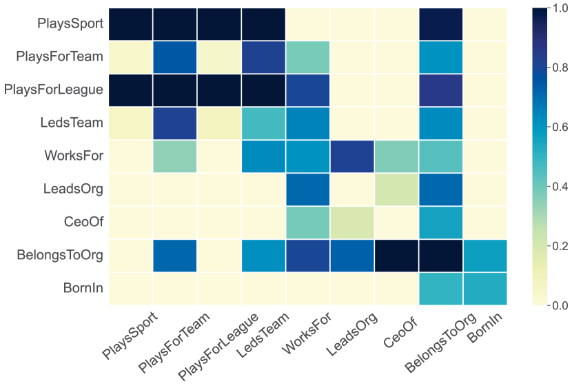
Figure 3. Feedback attentions of nine person-related relations from NELL-MBE. Each horizontal axis tick label is a query relation, and the vertical axis tick labels are the relations to be aggregated.

Heat map of feedback attentions. In this experiment, we take insight into how feedback attentions capture the varying correlation of relations regarding specific queries. In consideration of the readability, we choose several relations from NELL-MBE as examples for illustration. WN-MBE consists of conceptual-semantic and lexical relations of which the relation correlation is hard to measure, and the relations in FB-MBE are complex in structure and lack of readability. Specifically, we select nine person-related relations from NELL-MBE and show the feedback attentions between them in Fig. 3. The feedback attention mechanism encourages the agent to pay more attention to the query-related relations. For example, when answering the query ($e_{s}$, play_sport, ?), the irrelevant relations such as born_in would be assigned a small attention.

Case study. To demonstrate the reasoning ability of our model, we perform a case study on the trajectories that the agent walks. We take three sport-related queries also from NELL-MBE as examples, and compare the reasoning trajectories of our model and the second-best model GT. For each case, we do beam search with the evaluated model and treat the probability of searching each trajectory as the score of this trajectory. Table 12 presents the top-ranked trajectories and their scores. Note that we remove the self-loop actions for clarity. It can be seen from the three cases that our model reaches all gold target entities, but GT fails in the first two cases, which shows the superiority of our model. In Case 2, although the trajectory is long, our model still succeeds because ARGCN with feedback attention focuses on the correlation between relations and can better learn complex relational path patterns. In Case 3, both our model and GT reach the target entity, but our model is more confident about this trajectory. This is because the feedback attention is able to filter out noisy information for the query and make the action selection more stable.

Table 12. Case study. $r^{-}$ denotes the reverse relation of $r$. Target entities are underlined.

Case 1.	(xabi, athlete_home_stadium, stadium_anfield)	Scores
Ours	$\to$ (athlete_plays_for_team, team_liverpool)	0.37
	$\to$ (team_home_stadium, stadium_anfield)
GT	$\to$ (athlete_plays_for_team, team_liverpool)	0.14
	$\to$ (athlete_plays_for_team-, xabi)
Case 2.	(bowling_green_falcons, team_plays_in_league, ncaa)
Ours	$\to$ (agent_collaborates_with_agent, mexico_ncaa)	0.16
	$\to$ (agent_controls, unc_wilmington_seahawks)
	$\to$ (team_plays_in_league, ncaa)
GT	$\to$ (agent_collaborates_with_agent, mexico_ncaa)	0.12
Case 3.	(brett_carroll, athlete_plays_for_team, team_bobcats)
Ours	$\to$ (athlete_led_sports_team, team_bobcats)	0.17
GT	$\to$ (athlete_led_sports_team, team_bobcats)	0.04

6. Conclusion and Future Work

In this paper, we study a more challenging but realistic inductive KG reasoning scenario that new entities continually emerge in multiple batches and have sparse links. To address this new problem, we propose a novel walk-based inductive KG reasoning model. The experimental results on three newly constructed datasets show that our model outperforms the embedding-based, walk-based and rule-based competitors. In future work, we plan to study the reasoning task for expanding KG with emerging relations. We also want to investigate the effectiveness of our model in other applications such as multi-hop question answering.

Acknowledgments. This work was funded by National Natural Science Foundation of China (No. 62272219) and Collaborative Innovation Center of Novel Software Technology & Industrialization.

References

- (1)
- Baek et al. (2020) Jinheon Baek, Dong Bok Lee, and Sung Ju Hwang. 2020. Learning to Extrapolate Knowledge: Transductive Few-shot Out-of-Graph Link Prediction. In NeurIPS. Curran Associates, Inc., Vancouver, Canada, 546–560.
- Bhowmik and de Melo (2020) Rajarshi Bhowmik and Gerard de Melo. 2020. Explainable Link Prediction for Emerging Entities in Knowledge Graphs. In ISWC. Springer, Online, 39–55.
- Bordes et al. (2013) Antoine Bordes, Nicolas Usunier, Alberto García-Durán, Jason Weston, and Oksana Yakhnenko. 2013. Translating Embeddings for Modeling Multi-relational Data. In NeurIPS. Curran Associates, Inc., Lake Tahoe, NV, USA, 2787–2795.
- Carlson et al. (2010) Andrew Carlson, Justin Betteridge, Bryan Kisiel, Burr Settles, Estevam R. Hruschka Jr., and Tom M. Mitchell. 2010. Toward an Architecture for Never-Ending Language Learning. In AAAI. AAAI Press, Atlanta, GA, USA, 1306–1313.
- Chao et al. (2021) Linlin Chao, Jianshan He, Taifeng Wang, and Wei Chu. 2021. PairRE: Knowledge Graph Embeddings via Paired Relation Vectors. In ACL. ACL, Bangkok, Thailand, 4360–4369.
- Chen et al. (2021) Jiajun Chen, Huarui He, Feng Wu, and Jie Wang. 2021. Topology-Aware Correlations Between Relations for Inductive Link Prediction in Knowledge Graphs. In AAAI, Vol. 35. AAAI Press, Online, 6271–6278.
- Das et al. (2018) Rajarshi Das, Shehzaad Dhuliawala, Manzil Zaheer, Luke Vilnis, Ishan Durugkar, Akshay Krishnamurthy, Alex Smola, and Andrew McCallum. 2018. Go for a Walk and Arrive at the Answer: Reasoning Over Paths in Knowledge Bases using Reinforcement Learning. In ICLR. OpenReview.net, Vancouver, Canada, 18 pages.
- Dettmers et al. (2018) Tim Dettmers, Pasquale Minervini, Pontus Stenetorp, and Sebastian Riedel. 2018. Convolutional 2D Knowledge Graph Embeddings. In AAAI. AAAI Press, New Orleans, LA, USA, 1811–1818.
- Galárraga et al. (2015) Luis Galárraga, Christina Teflioudi, Katja Hose, and Fabian M. Suchanek. 2015. Fast Rule Mining in Ontological Knowledge Bases with AMIE+. The VLDB Journal 24, 6 (2015), 707–730.
- Galárraga et al. (2013) Luis Antonio Galárraga, Christina Teflioudi, Katja Hose, and Fabian M. Suchanek. 2013. AMIE: Association Rule Mining under Incomplete Evidence in Ontological Knowledge Bases. In WWW. ACM, Rio de Janeiro, Brazil, 413–422.
- Guo et al. (2019) Lingbing Guo, Zequn Sun, and Wei Hu. 2019. Learning to Exploit Long-term Relational Dependencies in Knowledge Graphs. In ICML, Vol. 97. PMLR, Long Beach, CA, USA, 2505–2514.
- Hamaguchi et al. (2017) Takuo Hamaguchi, Hidekazu Oiwa, Masashi Shimbo, and Yuji Matsumoto. 2017. Knowledge Transfer for Out-of-Knowledge-Base Entities: A Graph Neural Network Approach. In IJCAI. IJCAI, Melbourne, Australia, 1802–1808.
- Ji et al. (2021) Shaoxiong Ji, Shirui Pan, Erik Cambria, Pekka Marttinen, and S Yu Philip. 2021. A Survey on Knowledge Graphs: Representation, Acquisition, and Applications. IEEE Transactions on Neural Networks and Learning Systems 33, 2 (2021), 494–514.
- Lei et al. (2020) Deren Lei, Gangrong Jiang, Xiaotao Gu, Kexuan Sun, Yuning Mao, and Xiang Ren. 2020. Learning Collaborative Agents with Rule Guidance for Knowledge Graph Reasoning. In EMNLP. ACL, Online, 8541–8547.
- Lin et al. (2018) Xi Victoria Lin, Richard Socher, and Caiming Xiong. 2018. Multi-Hop Knowledge Graph Reasoning with Reward Shaping. In EMNLP. ACL, Brussels, Belgium, 3243–3253.
- Liu et al. (2021) Shuwen Liu, Bernardo Cuenca Grau, Ian Horrocks, and Egor V. Kostylev. 2021. INDIGO: GNN-Based Inductive Knowledge Graph Completion Using Pair-Wise Encoding. In NeurIPS. Curran Associates, Inc., Online, 2034–2045.
- Lv et al. (2019) Xin Lv, Yuxian Gu, Xu Han, Lei Hou, Juanzi Li, and Zhiyuan Liu. 2019. Adapting Meta Knowledge Graph Information for Multi-Hop Reasoning over Few-Shot Relations. In EMNLP. ACL, Hong Kong, China, 3376–3381.
- Meilicke et al. (2019) Christian Meilicke, Melisachew Wudage Chekol, Daniel Ruffinelli, and Heiner Stuckenschmidt. 2019. Anytime Bottom-Up Rule Learning for Knowledge Graph Completion. In IJCAI. IJCAI, Macao, China, 3137–3143.
- Rossi et al. (2021) Andrea Rossi, Denilson Barbosa, Donatella Firmani, Antonio Matinata, and Paolo Merialdo. 2021. Knowledge Graph Embedding for Link Prediction: A Comparative Analysis. ACM Transactions on Knowledge Discovery from Data 15, 2 (2021), 1–49.
- Sadeghian et al. (2019) Ali Sadeghian, Mohammadreza Armandpour, Patrick Ding, and Daisy Zhe Wang. 2019. DRUM: End-To-End Differentiable Rule Mining On Knowledge Graphs. In NeurIPS. Curran Associates Inc., Vancouver, Canada, 15321–15331.
- Schlichtkrull et al. (2018) Michael Schlichtkrull, Thomas N. Kipf, Peter Bloem, Rianne van den Berg, Ivan Titov, and Max Welling. 2018. Modeling Relational Data with Graph Convolutional Networks. In ESWC. Springer, Heraklion, Greece, 593–607.
- Shi and Weninger (2018) Baoxu Shi and Tim Weninger. 2018. Open-World Knowledge Graph Completion. In AAAI. AAAI Press, New Orleans, LA, USA, 1957–1964.
- Teru et al. (2020) Komal Teru, Etienne Denis, and Will Hamilton. 2020. Inductive Relation Prediction by Subgraph Reasoning. In ICML. PMLR, Online, 9448–9457.
- Toutanova and Chen (2015) Kristina Toutanova and Danqi Chen. 2015. Observed versus latent features for knowledge base and text inference. In CVSC. ACL, Beijing, China, 57–66.
- Vashishth et al. (2020a) Shikhar Vashishth, Soumya Sanyal, Vikram Nitin, Nilesh Agrawal, and Partha P. Talukdar. 2020a. InteractE: Improving Convolution-Based Knowledge Graph Embeddings by Increasing Feature Interactions. In AAAI. AAAI Press, New York, NY, USA, 3009–3016.
- Vashishth et al. (2020b) Shikhar Vashishth, Soumya Sanyal, Vikram Nitin, and Partha P. Talukdar. 2020b. Composition-based Multi-Relational Graph Convolutional Networks. In ICLR. OpenReview.net, Online, 16 pages.
- Vrandečić and Krötzsch (2014) Denny Vrandečić and Markus Krötzsch. 2014. Wikidata: A Free Collaborative Knowledgebase. Commun. ACM 57, 10 (2014), 78–85.
- Wan and Du (2021) Guojia Wan and Bo Du. 2021. GaussianPath: A Bayesian Multi-Hop Reasoning Framework for Knowledge Graph Reasoning. In AAAI. AAAI Press, Online, 4393–4401.
- Wan et al. (2020) Guojia Wan, Shirui Pan, Chen Gong, Chuan Zhou, and Gholamreza Haffari. 2020. Reasoning Like Human: Hierarchical Reinforcement Learning for Knowledge Graph Reasoning. In IJCAI. IJCAI, Yokohama, Japan, 1926–1932.
- Wang et al. (2021) Hongwei Wang, Hongyu Ren, and Jure Leskovec. 2021. Relational Message Passing for Knowledge Graph Completion. In KDD. ACM, Online, 1697–1707.
- Wang et al. (2019) Peifeng Wang, Jialong Han, Chenliang Li, and Rong Pan. 2019. Logic Attention Based Neighborhood Aggregation for Inductive Knowledge Graph Embedding. In AAAI. AAAI Press, Honolulu, HI, USA, 7152–7159.
- Wang et al. (2017) Quan Wang, Zhendong Mao, Bin Wang, and Li Guo. 2017. Knowledge Graph Embedding: A Survey of Approaches and Applications. IEEE Transactions on Knowledge and Data Engineering 29, 12 (2017), 2724–2743.
- Wang et al. (2014) Zhen Wang, Jianwen Zhang, Jianlin Feng, and Zheng Chen. 2014. Knowledge Graph Embedding by Translating on Hyperplanes. In AAAI. AAAI Press, Québec City, Canada, 1112–1119.
- Williams (1992) Ronald J Williams. 1992. Simple Statistical Gradient-Following Algorithms for Connectionist Reinforcement Learning. Machine Learning 8, 3–4 (1992), 229–256.
- Xiong et al. (2017) Wenhan Xiong, Thien Hoang, and William Yang Wang. 2017. DeepPath: A Reinforcement Learning Method for Knowledge Graph Reasoning. In EMNLP. ACL, Copenhagen, Denmark, 564–573.
- Yang et al. (2015) Bishan Yang, Wen-tau Yih, Xiaodong He, Jianfeng Gao, and Li Deng. 2015. Embedding Entities and Relations for Learning and Inference in Knowledge Bases. In ICLR. OpenReview.net, San Diego, CA, USA, 12 pages.
- Yang et al. (2017) Fan Yang, Zhilin Yang, and William W. Cohen. 2017. Differentiable Learning of Logical Rules for Knowledge Base Reasoning. In NeurIPS. Curran Associates Inc., Long Beach, CA, USA, 2319–2328.
- Yu et al. (2021) Donghan Yu, Yiming Yang, Ruohong Zhang, and Yuexin Wu. 2021. Knowledge Embedding Based Graph Convolutional Network. In WWW. ACM, Ljubljana, Slovenia, 1619–1628.
- Zhang et al. (2021) Yufeng Zhang, Weiqing Wang, Wei Chen, Jiajie Xu, An Liu, and Lei Zhao. 2021. Meta-Learning Based Hyper-Relation Feature Modeling for Out-of-Knowledge-Base Embedding. In CIKM. ACM, Queensland, Australia, 2637–2646.