Supplementary Material:
Neural Light Field Estimation for Street Scenes with Differentiable Virtual Object Insertion

In the supplementary material, we include additional details and results of our approach. We provide technical details in Section 1. We show additional auxiliary results which further ablate and explain our method in Section 2. We discuss limitations and broader impact in Section 3.

1 Implementation Details

1.1 Sky Modeling Architecture

The primary goal of the sky modeling neural network is to learn a low-dimensional feature space for the sky dome. The resulting network can also predict HDR information given input LDR panorama. The model architecture is illustrated in Figure A.

A 2D CNN encoder takes as input an LDR panorama with a positional encoding, and predicts the sky vector $\hat{\mathbf{f}}$ in the feature space. As each pixel in the panorama corresponds to a direction through equi-rectangular projection, the positional encoding $(\mathbb{R}^{3\times H\times W})$ encodes the directional information, where each pixel contains a unit vector indicating the direction of that pixel location. The decoder is a 2D UNet [15] decoding the sky vector into an HDR sky panorama. We carefully design its architecture to facilitate the reconstruction of the HDR sun peak. The input to the 2D UNet is a 7-channel panorama, including a 4-channel peak encoding and a 3-channel positional encoding, as shown in Figure A. Specifically, we embed the peak direction $\hat{\mathbf{f}}_{\text{dir}}$ information into a 1-channel peak direction encoding $\mathbb{R}^{1\times H\times W}$ with a spherical Gaussian lobe. For each pixel location corresponding to the direction $\mathbf{u}$, we compute the peak direction encoding as:

$$\text{PeakDirEncoding}(\mathbf{u})=e^{100(\mathbf{u}\cdot\hat{\mathbf{f}}_{\text{dir}}-1)}.$$ (1)

We encode the peak intensity into a 3-channel panorama by assigning the peak pixels to the predicted peak intensity $\hat{\mathbf{f}}_{\text{intensity}}$,

$$\text{PeakIntensityEncoding}(\mathbf{u})=\left\{\begin{aligned} &\hat{\mathbf{f}}_{\text{intensity}},&\ \ \text{if}\ \text{PeakDirEncoding}(\mathbf{u})\geq 0.98\\ &0,&\text{Otherwise}\end{aligned}\right.$$ (2)

This results in 7-channel input to the 2D UNet by concatenating the 1-channel peak direction encoding, 3-channel peak intensity encoding, and the 3-channel positional encoding used in the sky encoder. The sky latent code $\hat{\mathbf{f}}_{\text{latent}}$ is concatenated with the latent vector output by the 2D UNet to jointly decode the HDR sky dome.

The sky encoder contains two separate 2D CNNs with one predicting the peak information and the other predicting the latent code, where each CNN contains 5 downsampling conv-blocks with intermediate output channel dimensions of: $(64,128,256,256,256)$. For the sky decoder, the 2D UNet contains 5 downsampling conv-blocks and 5 upsampling conv-blocks, connected with residual links [8]. The intermediate output channel dimensions are $(64,128,256,256,256,256,128,64,32,16)$. Each conv-block contains two 2D convolution layers followed by batch normalization and ReLU activation.

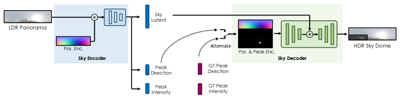
Figure A: Architecture of our sky modeling network. The encoder takes as input an additional positional encoding, concatenated with the input LDR panorama. We compute a panorama image encoding peak and positional information, and feed it into a 2D UNet [15] decoder. The sky latent code is fused in the latent space of the decoder. During training, we alternate between end-to-end training and teacher forcing.

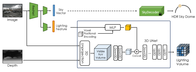
Figure B: Architecture of our hybrid lighting prediction network. For HDR sky dome prediction (top), we directly predict the sky feature vector from the ResNet backbone. For lighting volume prediction (bottom), inspired by [20], we unproject the 2D input image into a 3D volume and process it with a 3D UNet. The global lighting feature is converted to a feature volume with an MLP and later fused into the 3D UNet.

1.2 Hybrid Lighting Prediction Architecture

The 2D CNN backbone for the Hybrid Lighting Joint Prediction module (depicted in Figure B and main paper Figure 2(a)) is ResNet50 [8], with two separate branches predicting the sky feature vector and the scene lighting feature.

For the sky prediction branch, the sky feature vector $(\mathbb{R}^{64})$ is then passed into the pre-trained sky decoder, with frozen weights, to decode the HDR sky dome $(\mathbb{R}^{3\times 64\times 256})$.

We adapt the architecture used in [20] for the lighting volume prediction branch. To encode the visible field-of-view (FoV) information, we unproject the input image into the initial visible surface volume $(\mathbb{R}^{4\times 64\times 256\times 256})$ [20]. The scene lighting feature $(\mathbb{R}^{128})$ extracted with the ResNet backbone is passed into a coordinate MLP [16], and decoded into a global scene feature volume $(\mathbb{R}^{32\times 16\times 64\times 64})$. Here, the coordinate network [16] contains three residual MLP blocks and the hidden size is $64$. We use 3D UNet [15] to process the visible surface volume $(\mathbb{R}^{4\times 64\times 256\times 256})$, which contains five downsampling and upsampling conv-blocks with residual connections [8], and each conv-block contains two 3D convolution layers. The global scene feature volume $(\mathbb{R}^{32\times 16\times 64\times 64})$ is fused into the 3D UNet after 2 downsampling conv-blocks. The intermediate output channels of each conv-block have dimensions of $(12,16,32,128,256,256,128,64,32,16)$. The final conv-layer produces the lighting volume prediction $(\mathbb{R}^{8\times 64\times 256\times 256})$.

1.2.1 Pre-trained depth estimation.

In this work, we rely on the existing state-of-the-art off-the-shelf monocular depth estimator PackNet [7] to obtain the 2.5D geometry of the scene. We empirically find that the depth perception is robust with reasonable performance, and provide analysis on the influence of depth prediction error below.

The predicted depth is first used in lighting volume prediction, where the scene pixel values are unprojected into 3D with the depth prediction. More accurate depth prediction informs more precise geometric information of the scene, and will improve the performance of lighting estimation, e.g. the quantitative metric in main paper Table 2.

Then, during differentiable object insertion, we use depth to decide on the 3D placement of the object we want to insert. Since the location of the inserted object is computed from the depth map, the scale error of the depth prediction leads to error in the size of the inserted objects. To address this, we use the projected sparse LiDAR points as ground-truth depth to rescale the estimated depth by minimizing the L2 error between them.

When rendering shadows of the inserted object, we rely on the pre-computed depth to compute the 3D location of each scene pixel, which is needed to perform the ray-mesh queries. Thus, errors in the estimated depth may result in incorrect shadows. We empirically find that this error is usually negligible as we insert mostly on flat surfaces.

Prior works that contain submodules with depth prediction [14, 20] typically do not focus on improving depth perception, but simply use synthetic data with paired ground-truth to train the depth estimation branch, which may easily suffer from the domain gap. With a focus on lighting estimation and realistic object insertion, we believe that using the existing mature depth prediction models as a building block is a plausible design choice and does not decrease our technical contribution.

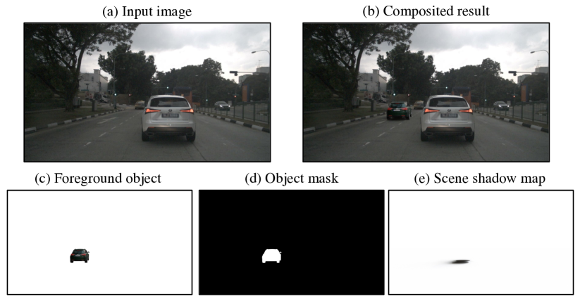
Figure C: Visualization of object insertion composition. Given an input image (a), we estimate our hybrid lighting representation. We render the foreground inserted object with standard deferred rendering [3] and obtain the rendering result (c) and object mask (d). We render the shadow cast by the inserted object into a ratio map (e) as described in main paper Section 3.3. The final editing result (b) is produced by compositing (c-e).

1.3 Differentiable Object Insertion

We visualize the object insertion composition process in Figure C. We composite the input image $I$, foreground object $I_{\text{object}}$, alpha mask $M$, scene shadow map $I_{\text{shadow}}$ into the final editing result $I_{\text{edit}}$ by

$$I_{\text{edit}}=M\odot I_{\text{object}}+(1-M)\odot I\odot I_{\text{shadow}}.$$ (3)

We include the implementation details below.

1.3.1 Rendering details.

For rendering the foreground object, we use the BRDF used by Unreal Engine 4, which is a simplified version of Disney BRDF [1, 12]. Specifically, we use the base color $c_{\text{base}}\in\mathbb{R}^{3}$, metallic $m\in[0,1]$, roughness $r\in[0,1]$ and specular $s\in[0,1]$ to describe material properties of object surfaces. The BRDF is defined as

$$f(\mathbf{l},\mathbf{v})=\frac{c_{\text{diffuse}}}{\pi}+\frac{DFG}{4(\mathbf{n}\cdot\mathbf{l})(\mathbf{n}\cdot\mathbf{v})},$$ (4)

where

$$c_{\text{diffuse}} =(1-m)\,c_{\text{base}}$$ (5)

$$c_{\text{specular}} =(1-m)\,0.08s+m\,c_{\text{base}}$$ (6)

$$D =\frac{\alpha^{2}}{\pi((\mathbf{n}\cdot\mathbf{h})^{2}(\alpha^{2}-1)+1)^{2}}$$ (7)

$$G =\frac{(\mathbf{n}\cdot\mathbf{l})(\mathbf{n}\cdot\mathbf{v})}{((\mathbf{n}\cdot\mathbf{l})(1-k)+k)((\mathbf{n}\cdot\mathbf{v})(1-k)+k)}$$ (8)

$$F =c_{\text{specular}}+(1-c_{\text{specular}})2^{(-5.55473(\mathbf{v}\cdot\mathbf{h})-6.98316)(\mathbf{v}\cdot\mathbf{h})}$$ (9)

$$\alpha =r^{2},k=\frac{(r+1)^{2}}{8},\mathbf{h}=\frac{\mathbf{l}+\mathbf{v}}{||\mathbf{l}+\mathbf{v}||}.$$ (10)

The rendered raw pixel values is HDR in linear RGB space. To convert to LDR sRGB images, we apply gamma correction ($\gamma=2.2$), and do soft clipping following [20]

$$\varphi(x)=\left\{\begin{aligned} &x&\text{if}\ x\leq\tau\\ &1-(1-\tau)e^{-\frac{x-\tau}{1-\tau}}&\text{if}\ x>\tau\end{aligned}\right.$$ (11)

where we set $\tau=0.95$.

During training, to save on the computational cost and GPU memory, we uniformly sample $5000$ rays for object center alone, and render the foreground object on a 320x180 image canvas. For background shadows, we render a 160x90 resolution shadow map. We sample $50$ rays for each scene pixel, and aggregate the 8-neighbors of each pixel to obtain $450$ rays in total. The average rendering time for foreground objects and background shadows are 0.2s and 2s respectively. The current efficiency bottleneck in the renderer is the ray-mesh query function, which is a CPU implementation using trimesh with the potential to further speedups. It consumes 12G GPU memory during training, including both the forward and the backward pass. During inference, we sample rays for each object pixel using per-pixel importance sampling following [3] to achieve high quality rendering, where we sample 1024 rays for the diffuse component and 256 rays for the specular component.

1.3.2 Ray sampling scheme.

A larger number of ray samples may lead to higher quality rendering, but usually limited by the affordable memory and computation, especially for a differentiable rendering module in end-to-end learning tasks. To improve the efficiency of ray sampling especially for the process of shadow rendering, we select equi-spaced rays for each pixel on the upper-hemisphere with Fibonacci lattice [6] to render the spatially-varying shadows. As shown in Figure D, the Fibonacci lattice ray selection strategy better utilizes the rays compared to naive uniform sampling.

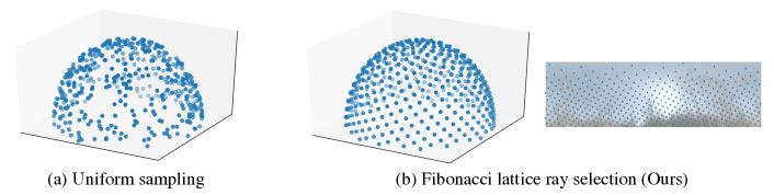
Figure D: Visualization of ray directions. Instead of using naive uniform ray sampling (a), we select equi-spaced rays with Fibonacci lattice (b). This scheme better utilizes the rays and can ensure the sun light is properly sampled.

1.3.3 Object insertion details.

During training, we use the task of object insertion to provide additional supervision. Specifically, we differentiably insert a virtual object into the photograph and encourage the photorealism of the final image editing results. We adopt a relatively conservative scheme to avoid unrealistic editing results due to asset quality and object placement. For assets, we collect a set of 283 high quality 3D car models from Turbosquid. To place the cars into plausible locations, we use the dense depth map prediction [7], lidar semantic segmentation and 3D bounding box annotation in nuScenes [2]. The location candidates for insertion should satisfy the following conditions: (1) Semantics: belong to the semantic class “driveable surface”, (2) Distance: within the range of 10 to 40 meters, (3) Collision: candidate location is 1 meter away from the static background classes (such as “sidewalk”) and 3 meters away from dynamic classes (such as “vehicles”), and (4) Occlusion: the 3D bounding box corners of the inserted object do not get occluded by other objects. The car orientation is randomly set to the same or opposite direction as the ego camera, with a Gaussian random perturbation in the yaw angle (sigma value set to $3^{\circ}$).

1.3.4 Object insertion for data augmentation.

For downstream tasks, we use object insertion as a data augmentation approach, to enhance the data with additional diversity. We use the 283 car CAD models and randomize the car paint with 60 diverse colors. For diversity, we also include 30 high quality construction vehicle CAD models that are rarely observed on the street. We remove the occlusion check mentioned above, and naively handle the occlusion by comparing the depth map of the scene and inserted object. For orientation, we increase the Gaussian perturbation with sigma value set to $15^{\circ}$.

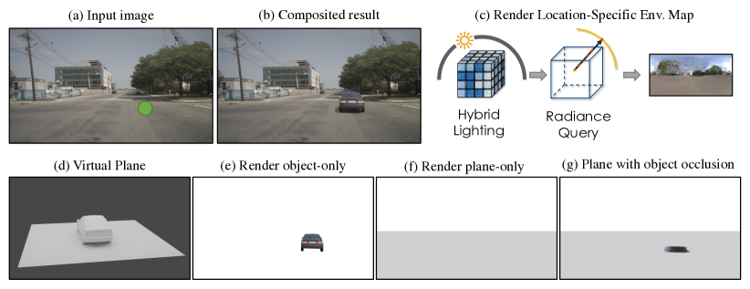
Figure E: Rendering object insertion with Blender. Our lighting representation can be converted to the standard environment map to be compatible with commercial renderers (thus gaining the benefits of richer material support and speed of commercial renderers). Given the input image (a) and the 3D location shown in green to insert object, we first convert our hybrid lighting into a local environment map with volume rendering (c). We place a virtual plane under the inserted object (d), and render three images – Object-only (e), plane-only (f) and plane with object occlusion (g). The shadow map can be computed by the ratio of (f) and (g). The final editing result is shown in (b).

1.3.5 Rendering object insertion with commercial renderer.

While we adopt our proposed custom differentiable object insertion module during training to provide valuable supervision signal, our rendering is fully physics-based with standard PBR material definition. Thus, our estimated lighting can also be made useable in commercial rendering engines such as the Cycles renderer in Blender [5]. This allows us to utilize faster rendering as well as richer material support available in the commercial renderers.

Commercial renderers usually only support standard environment map lighting and do not support spatially-varying lighting such as our hybrid lighting representation. In addition, the radiance-level API is not available for shadow rendering. We modify our object insertion pipeline to be compatible with Blender Cycles renderer in Figure E. Given the 3D location to insert the virtual object, we first render our lighting representation into a standard HDR environment map by doing radiance query at the specified 3D location (main paper Eq. 1), and load into Blender as lighting. To render cast shadows, we insert a virtual plane beneath the inserted object, and render three images: (1) render only inserted object $I_{\text{object}}$, (2) render only virtual plane $I_{\text{plane}}$, (3) render the virtual plane but take into account of the inserted object when doing ray-tracing $I_{\text{shadowed}}$. The shadow map can be computed as $I_{\text{shadow}}=\frac{I_{\text{shadowed}}}{I_{\text{plane}}}$, followed by the image composition in Figure C. Note that this maximally preserves scene-level spatially-varying effects, but still ignores the local geometry of object and virtual plane, and thus cannot render localized shadow effects as shown in main paper Figure 6.

We show qualitative results from Blender in Figure N. In most cases, with the Cycles renderer at inference time, we can benefit from more bounces of ray-tracing and complex materials such as transparency and sub-surface scattering.

1.4 Training Details

1.4.1 Sky modeling network.

We use a multi-task loss to train the sky encoder-decoder network:

$$\mathcal{L}^{\text{skym}}=\lambda_{\text{dir}}\mathcal{L}_{\text{dir}}^{\text{skym}}+\lambda_{\text{intensity}}\mathcal{L}_{\text{intensity}}^{\text{skym}}+\lambda_{\text{hdr}}\mathcal{L}_{\text{hdr}}^{\text{skym}}$$ (12)

where the weights are all set to 1. During training, we introduce “teacher forcing” on HDR reconstruction loss $\mathcal{L}_{\text{hdr}}$ by alternating the input to sky decoder between $(\hat{\mathbf{f}}_{\text{dir}},\hat{\mathbf{f}}_{\text{intensity}},\hat{\mathbf{f}}_{\text{latent}})$ and $({\mathbf{f}}_{\text{dir}},{\mathbf{f}}_{\text{intensity}},\hat{\mathbf{f}}_{\text{latent}})$. This is because the prediction of the peak direction $\hat{\mathbf{f}}_{\text{dir}}$ and peak intensity $\hat{\mathbf{f}}_{\text{intensity}}$ are usually inaccurate in the early stages of training. This also helps to efficiently disentangle the peak and the background (Figure I), encouraging the network to accurately reconstruct HDR peak when given groundtruth peak information ${\mathbf{f}}_{\text{dir}},{\mathbf{f}}_{\text{intensity}}$. We use the Adam optimizer [13] and train for 4000 epochs, with the learning rate set to 1e-3 and decaying by $0.3$ every 1000 epochs.

1.4.2 Lighting prediction network.

We use a weighted sum of loss terms introduced in the main paper in Section 3.4, including the sky regression loss $\mathcal{L}_{\text{sky}}$, radiance and depth reconstruction loss $\mathcal{L}_{\text{recon}}$, sky separation loss $\mathcal{L}_{\text{transmit}}$, and adversarial supervision $\mathcal{L}_{\text{adv}}$. To address the ambiguity of depth rendering, we also follow [20] and use a regularization loss $\mathcal{L}_{\text{reg}}$ to encourage the alpha channel of the volume to be either 0 or 1. The final loss function

$$\mathcal{L}^{\text{hybrid}}=\lambda_{\text{sky}}\mathcal{L}_{\text{sky}}+\lambda_{\text{recon}}\mathcal{L}_{\text{recon}}+\lambda_{\text{reg}}\mathcal{L}_{\text{reg}}+\lambda_{\text{transmit}}\mathcal{L}_{\text{transmit}}+\lambda_{\text{adv}}\mathcal{L}_{\text{adv}}$$ (13)

where we set $\lambda_{\text{sky}},\lambda_{\text{recon}},\lambda_{\text{transmit}}$ to 1, $\lambda_{\text{reg}}$ to 1e-4, and $\lambda_{\text{adv}}$ to 3e-3. For the sky regression loss $\mathcal{L}_{\text{sky}}$, we linearly fade out the L1 loss for latent code in the first 50 epochs. For the adversarial supervision $\mathcal{L}_{\text{adv}}$, the discriminator $\mathcal{D}$ is a 5-layer PatchGAN with spectral norm [11, 18]. We use hinge loss for the discriminator

$$\mathcal{L}^{\text{D}}= \max(0,1-\mathcal{D}(I_{\text{real}}))+\max(0,1+\mathcal{D}(\hat{I}_{\text{edit}})).$$ (14)

where we use the training set of real world images $\{I_{\text{real}}\}$ from nuScenes [2] and perspective image crops from HoliCity street views [22] as positive examples. We set the batch size to 1. The full model takes 20G GPU memory during training (8G for network inference and 12G for rendering). We first pre-train without $\mathcal{L}_{\text{adv}}$ for 50 epochs and then jointly train another 50 epochs. We train with the Adam optimizer [13] with learning rate of 3e-4, decaying by $0.3$ every 30 epochs.

1.5 Experimental Settings

1.5.1 Data processing.

We train our model on nuScenes [2], HoliCity [22], and a set of 724 outdoor HDR panoramas collected from three data sources: HDRIHaven, DoschDesign and HDRMaps. For HDRI data, we use 90% and 10% for training and evaluation. During training, we apply random flipping and random azimuth shifting as data augmentation. For nuScenes, we use the official split containing 700 scenes for training and 150 scenes for evaluation. For each key frame, we take the front camera as the input image and use the captured views at a novel viewpoint (1.5 seconds after the input frame) to supervise lighting. For HoliCity dataset, we follow [10] and detect the sun location as the centriod of largest connected region after thresholding with the 98-th percentile. For evaluation, we manually annotated the sun location for the test set. Considering that the peak direction is ambiguous for an almost uniform sky dome, we only use a subset of the HoliCity data with a strong peak to train and evaluate the peak direction prediction. Specifically, we pass the LDR panoramas to the pre-trained sky encoder and get the intensity prediction $\tilde{\mathbf{f}}_{\text{intensity}}$. Loss is only used when the peak intensity is greater than 10. This results in 1897 panoramas for training and 183 panoramas for evaluation.

1.5.2 Human perception study details.

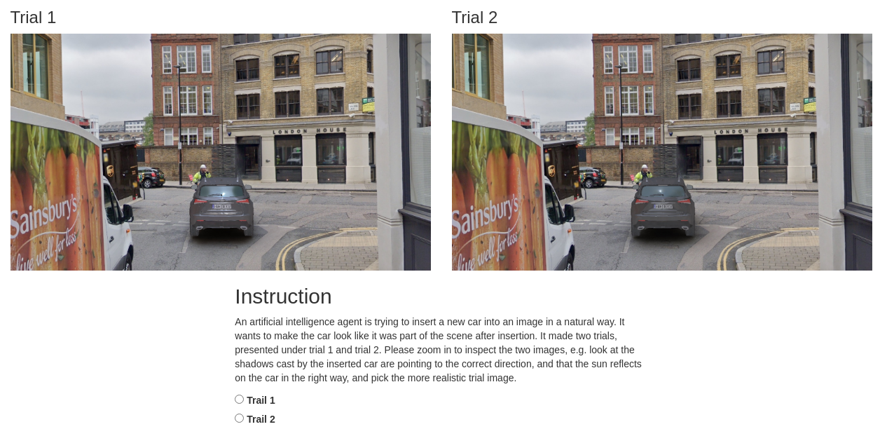
Figure F: User Study Interface (AMT): We insert two cars, which are rendered with different lighting approaches, into the same background image, and ask a human participant to select the more realistic one. We conduct 3 comparisons, where we first compare our full model with the baseline lighting methods [20, 9], then ablate against our method without adversarial supervision. We randomize their order in each HIT.

In this section, we provide additional details of our user study. We perform the user study on Amazon Mechanical Turk (AMT) and visualize the interface in Figure F. In each HIT, we provide two images and ask the user to select the more realistic one. Among the two images, one is relighted by our approach and the other is either one of the baselines [20, 9] or the ablation setting (Ours w/o adversarial supervision). To avoid bias in order, we always randomize which of the methods is shown on the left vs right. We provide instructions as follows:

An artificial intelligence agent is trying to insert a new car into an image in a natural way. It wants to make the car look like it was part of the scene after insertion. It made two trials, presented under trial 1 and trial 2. Please zoom in to inspect the two images, e.g. look at the shadows cast by the inserted car are pointing to the correct direction, and that the sun reflects on the car in the right way, and pick the more realistic trial image.

We synthesize 23 insertion examples. For each example, we ask 15 users to judge the realism of the inserted object and adopt a majority vote to compute the final preference. In summary, it results in $3\text{ comparisons}\times 23\text{ examples}\times 15\text{ selections}\times 3\text{ repeat experiments}=3105\text{ HITs}$. We provide results in Table 3 in the main paper, demonstrating that users prefer our approach over the baselines [20, 9], and adding adversarial supervision further improves the realism of object insertion.

2 Additional Results

2.1 Sky modeling

The sky encoder-decoder takes as input an LDR sky panorama, and produces a low-dimensional vector representation of the sky $\hat{\mathbf{f}}$ and a reconstructed HDR sky dome. The qualitative results are shown in Figure I. Our model can accurately reconstruct HDR sky, especially the peaks with extreme intensity values. As the sky vector $\hat{\mathbf{f}}=(\hat{\mathbf{f}}_{\text{intensity}},\hat{\mathbf{f}}_{\text{dir}},\hat{\mathbf{f}}_{\text{latent}})$ contains explicit peak information, it enables peak editing by feeding into edited sky vector $(\hat{\mathbf{f}}_{\text{intensity}}^{\text{edit}},\hat{\mathbf{f}}_{\text{dir}}^{\text{edit}},\hat{\mathbf{f}}_{\text{latent}})$. As the results shown, our sky decoder can efficiently disentangle the HDR peak from the background, and enables precise peak editing. The controllable property allows for potential post-editing of inaccurate predictions.

We quantitatively ablate our architecture design and show the results in Table A. We evaluate by comparing the MSE of reconstructed HDR sky dome and the ground truth, and the median angular error between the reconstructed peak and the ground-truth peak direction. For the ablated version, “ours w/o encoding” removes the positional encoding and peak encoding concatenated to the Sky Encoder and Sky Decoder, and “ours w/o peak information” removes the peak direction and peak intensity and only relies on the latent code to reconstruct HDR sky. The quantitative results validated the effectiveness of our design choices to achieve the best performance. We also compare under the same experiment setting with the sky representation used in [9], where the HDR sky is represented with a latent vector and explicit azimuth of the sun. Our method outperforms [9], which shows the benefits from the explicit representation and supervision of peak direction and intensity.

Method	HDR reconstruction MSE $(\times 10^{-2})$ $\downarrow$	Peak direction median angular error $\downarrow$
Latent code w/ explicit azimuth [9]	$10.56$	$5.67^{\circ}$
Ours	$\bm{7.49}$	$\bm{3.38}^{\circ}$
Ours (w/o encoding)	$8.31$	$4.09^{\circ}$
Ours (w/o peak information)	$11.01$	$7.93^{\circ}$

Table A: Quantitative results of sky modeling. We compare the HDR reconstruction MSE and the median angular error of the reconstructed peak direction.

2.2 Auxiliary Quantitative Evalutation of Lighting Estimation

Prior works [21] that ignore spatially-varying effects may also enforce that a known rendered virtual scene $\mathcal{O}_{\text{scene}}$ (e.g. a sphere) appears consistent when using the predicted envenvironment map and groundtruth envenvironment map, i.e., $||\text{Render}(L_{\text{pred}},\mathcal{O}_{\text{sphere}})-\text{Render}(L_{\text{gt}},\mathcal{O}_{\text{sphere}})||$. Compared to the direct envenvironment map regression loss $||L_{\text{pred}}-L_{\text{gt}}||$, this is still regression but smartly weighted. This can be used as both training loss and evaluation metric, when prior works simplify the lighting to only one environment map.

However, for spatially-varying lighting estimation which is the focus of our work, there is no groundtruth lighting provided for the specific 3D location of the inserted object, and thus we cannot directly utilize this as a training loss.

Despite not a precise metric, we show the quantitative evaluation of this metric as an auxiliary result. Specifically, we take a cropped perspective image of groundtruth HDR panorama as input, and insert a diffuse or specular sphere with the estimated lighting. We report MSE between insertion results generated with predicted lighting and groundtruth HDR panorama, as shown in Table. B. Hold-Geoffroy et al. [9] ignores spatially-varying effects and usually cannot recover the high-frequency details, and thus lead to inferior performance on specular sphere insertion. Wang et al. [20] cannot reconstruct the HDR component well and especially suffers when inserting a diffuse sphere. Our method outperforms baselines with better quantitative performance.

Rendering MSE ($\times 10^{-3}$) $\downarrow$	Diffuse Sphere	Specular Sphere
Hold-Geoffroy et al. [9]	2.30	4.44
Wang et al. [20]	3.36	3.13
Ours	1.79	2.41

Table B: Rendering error of inserted objects. Note that this evaluation ignores spatially-varying effects.

2.3 Quantitative Ablation of Multi-view Input

While we focus on monocular estimation, our model is extendable to multi-view input, such as the six surrounding perspective cameras in nuScenes sensor rig [17]. For extremely challenging cases such as predicting precise shadow boundaries, multi-view input images can provide more field-of-view information and predict more accurate lighting, as shown in main paper Figure 6. We additionally provide quantitative result in Table C, following the experiment settings in main paper Table 1, 2. Although the six surrounding views still only cover a subset of the panorama, it can significantly improve upon monocular lighting prediction.

Method	HoliCity [22] sun location Median angular error $\downarrow$	nuScenes [2] PSNR $\uparrow$	nuScenes [2] si-PSNR $\uparrow$
Ours	$22.43^{\circ}$	$14.49$	$15.35$
Ours (6 views)	$\bm{19.91}^{\circ}$	$\bm{17.96}$	$\bm{18.45}$

Table C: Quantitative ablation study of multi-view input.

2.4 Analysis of the Adversarial Supervision

The adversarial supervision (main paper Section 3.4, Training Lighting via Object Insertion) uses a discriminator to encourage the photorealism of the lighting-aware image editing results, where this signal is backpropagated to the predicted lighting through the Differentiable Object Insertion module (main paper Section 3.3).

To understand the “photorealism” implicitly perceived by the discriminator during the training process, we perform test-time optimization on the object insertion results and visualize the optimization process (main paper Figure 7). Specifically, we take the network weights of the lighting prediction network $\Theta$ and the discriminator $\mathcal{D}$ in the middle of the training process (10-th epoch), and optimize the lighting prediction network weights $\Theta$ to minimize the discriminator loss $\mathcal{L}_{\text{adv}}=-\mathcal{D}(\hat{I}_{\text{edit}})$. Note that the discriminator and the pre-trained sky decoder are kept frozen.

We use Adam optimizer [13] with learning rate 1e-4, and show the optimized results after 5 and 10 iterations in Figure O. We refer to the accompanied video for animated results.

In high-level, the scene appearance (encoded by image pixel values) is an interaction between scene geometry, material and lighting, where this process can be approximated by the rendering equation. With known groundtruth image distribution implicitly learned with a discriminator, we utilize groundtruth material and geometry to supervise lighting prediction, by inserting artist-designed virtual objects into the scene images. This objective matches the end goal of our predicted lighting – the photorealism of image editing results. Both quantitative results and qualitative visualization indicate its value as a complementary supervision signal to existing datasets.

2.5 Improving Downstream Perception with Data Augmentation

2.5.1 Qualitative results of data augmentation.

We show the augmented data using our AR pipeline in Figure J, K, L, M. The 3D assets are provided courtesy of TurboSquid and their artists Hum3D, be fast, rabser, FirelightCGStudio, amaranthus, 3DTree_LLC, 3dferomon and Pipon3D. Note that the 3D bounding box and orientation of the inserted objects are known and become free labels to train a 3D object detector.

As shown in Figure J, our data augmentation inserts a diverse set of car assets into captured images from the nuScenes dataset [2] based on the estimated lighting. The data generation process is fully automatic. Our editing results can produce realistic lighting effects, such as cast shadows, which requires accurate HDR prediction, and “clear coat” reflection on the car body, which requires high-frequency lighting prediction and HDR highlights.

While many existing image manipulation methods [4, 17] have underlying assumptions about object categories, our method predicts physics-based scene lighting information, and thus is agnostic to the category of the virtual object to insert. This enables editing with object classes rarely observed in real world – a critical use case for data augmentation. Figure K shows insertion results of construction vehicles, where our method demonstrates consistent performance.

In Figure L, we show results of occlusion handling. We adopt a simple strategy by comparing the depth of the inserted object (cached in G-buffer) with the scene depth map, and take the closer pixel to display.

While we primarily focus on daytime outdoor scenes, our method can also predict reasonable results for night-time scenes, as shown in Figure M. Note that our model has no HDR data supervision for this domain, due to the scarcity of ground truth lighting for night time street scenes, and only relies on limited FoV LDR data and the adversarial supervision to learn.

2.5.2 Quantitative results.

We compare against the baseline that uses real-world data only, and a strong baseline that augments virtual objects with a fixed dome lighting. In Table D, we can observe that the performance of the detector improves by $2\%$ comparing to the same detector when trained on real data alone. Moreover, we can also see that while naively adding objects leads to a $1\%$ improvement, another $1\%$ is a result of having better light estimation. We believe that further improvements are possible with more sophisticated placement strategies as well as using more assets (both for each class, and more classes). Interestingly, notice that the performance of the object detector also improves in other object categories even though we do not directly augment those. We attribute this to various factors, including providing the detector with more challenging negatives for other classes, improving the detector’s confidence in classes that may get confused with construction vehicles (e.g. bus vs construction vehicles and trailer vs construction vehicles), as well as the way certain objects are annotated. For example, we notice that cranes and extremities of construction vehicles are only included in nuScenes annotations if they interfere with traffic (see Figure H), therefore what constitutes a 3D bounding box for that object category is not uniquely defined. We additionally notice that in nuScenes trucks used to hauling rocks or building materials are considered as truck rather than construction vehicles. These factors might also explain why we do not see a big improvement in the class of construction vehicles even though we directly augment it.

Method	mAP	car	truck	bus	trailer	const.veh.	pedestrian	motorcycle	bicycle	traffic cone	barrier
Real Data	0.190	0.356	0.112	0.124	0.011	0.016	0.327	0.127	0.116	0.389	0.317
+ Aug No Light	0.201	0.363	0.149	0.163	0.029	0.021	0.311	0.146	0.120	0.394	0.309
+ Aug Light	0.211	0.369	0.146	0.182	0.036	0.020	0.317	0.161	0.146	0.400	0.332

Table D: Performance of a SoTA 3D object detector on the nuScenes 3D object detection task. mAP represents the mean for the 10 object categories. We additionally report the average precision (AP) for all categories. Real Data corresponds to a subset of the nuScenes training set (10%). Performance of the detector improves by $2\%$ when comparing to Real Data, and 1% is due to better lighting estimation.

(a) Model Trained on Real Data	(b) Model Trained on Real Data + Lighting Aug

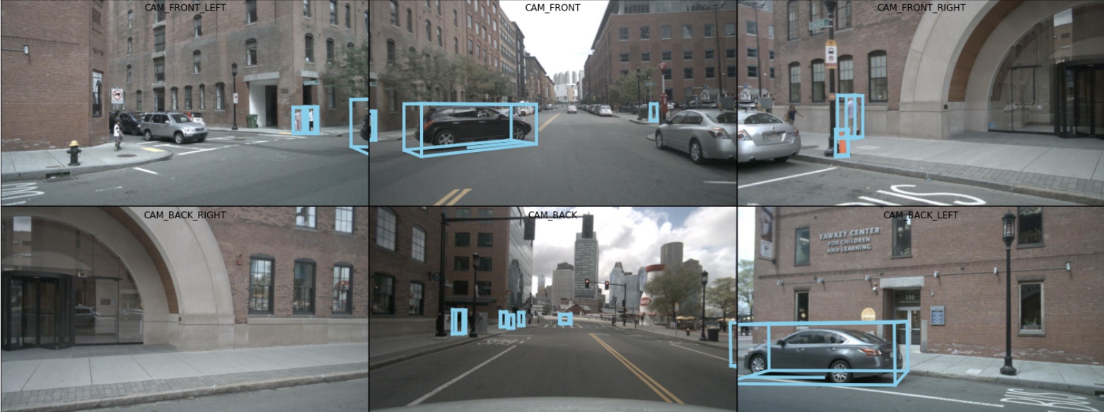
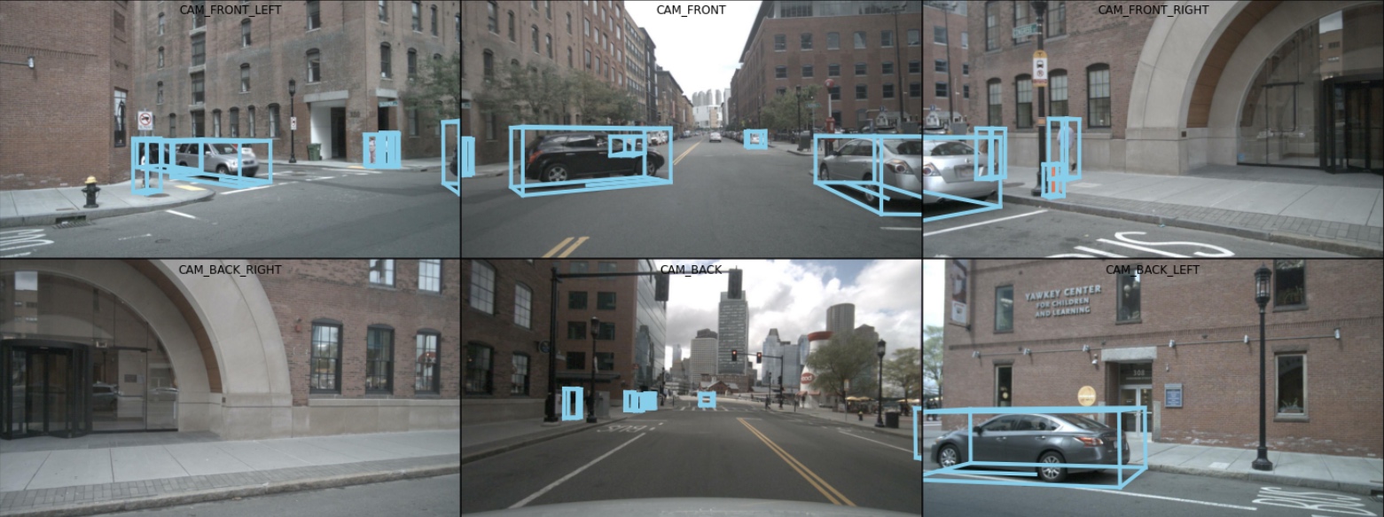
Figure G: Downstream 3D Detection. (a) Results of a 3D object detector trained on Real Data. (b) Results of the same detector trained on Real Data + Aug Lighting. We obtain improved detections after training on data generated with our method.

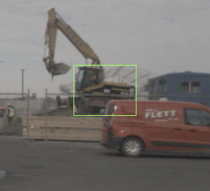
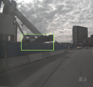
Figure H: Example of nuScenes annotations of construction vehicles. Extremities of construction vehicles are only included in nuScenes annotations if they interfere with traffic. Therefore, 3D bounding boxes for that object category are not uniquely defined.

3 Discussion

3.0.1 Failure cases and future works.

We show failure cases of our method in Figure P and describe below.

In our current object insertion pipeline, the inserted object pixels will not pass exactly the same image capturing process as the background scene pixels, and thus cannot simulate the sun halo effects and blurry rain-drop effects. In addition, a better modeling of the camera image signal processor (ISP) pipeline, such as tone-mapping, could potentially lead to more realistic object insertion. We believe it is an interesting future work to learn camera sensor parameters, and handle the diverse weather such as rainy, snowy and foggy effects.

With unknown scene material properties, our current shadow map rendering (main paper Eq. 4) assumes a Lambertian scene surface. This assumption enables measuring the residual effects caused by the inserted object with a ratio image. Although the Lambertian assumption is usually a good approximation and widely adopted in prior works [19, 20], the shadow map quality will decrease when this assumption no longer holds. For example, the wet road surfaces in rainy days become quite specular and should reflect the appearance of the inserted object, as shown in the second column of Figure P. It is an interesting direction to jointly estimate scene material properties to address such complex effects. In the third column of Figure P, our editing results exhibit occlusion artifacts when the scene depth map is inaccurate. While predicting more accurate depth is out of the scope of our paper, we believe an additional geometry refinement adopted in prior works [4] could be beneficial to address this issue.

3.0.2 Broader impact.

Our paper focuses on a neural Augmented Reality (AR) pipeline for outdoor scenes, which first estimates the lighting information and insert virtual objects into the input image. We show that our carefully designed hybrid lighting representation handles both the spatially-varying effects and the extreme HDR intensity of outdoor scenes. The differentiable object insertion formulation with an adversarial discriminator serves as a valuable supervision signal, which for the first time enables lighting supervision by jointly leveraging ground truth material, geometry and real world images. We show the benefits of our AR approach on a downstream 3D object detector, indicating its potential as a valuable data augmentation technique for safety-critical applications such as autonomous driving.

Our method falls into the category of works that enable image editing. While we believe that there are many positive implications, however – just like with the deep fake technology, we can also foresee nefarious use cases, such as rendering offensive content into photographs. Technology targeting detecting offensive content could help alleviate such use cases.

	Example 1	Example 2
Input LDR & GT HDR
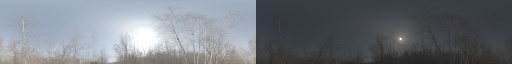
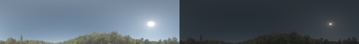
Reconstructed HDR sky
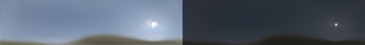
Peak direction editing
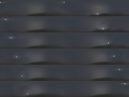
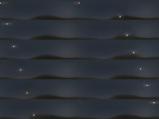
Input LDR & GT HDR
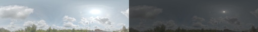
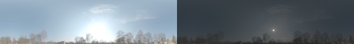
Reconstructed HDR sky
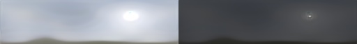
Peak direction editing
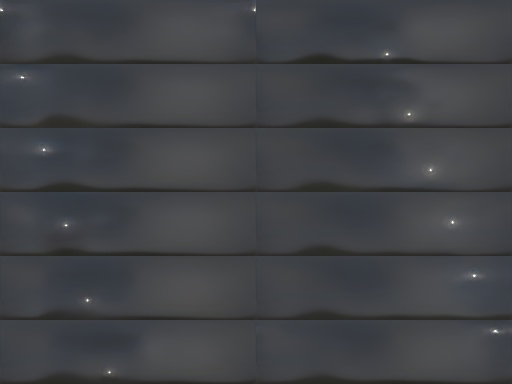
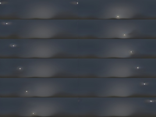
Input LDR & GT HDR
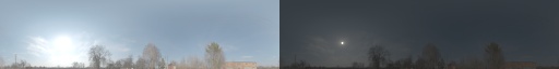
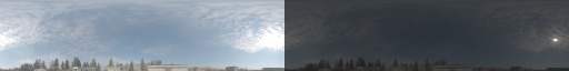
Reconstructed HDR sky
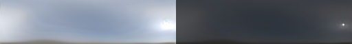
Peak direction editing

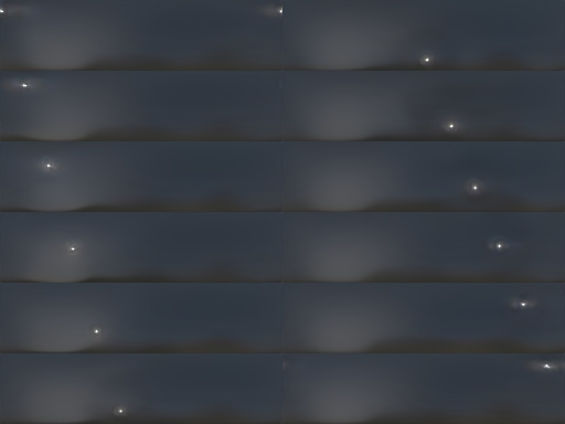
Figure I: Qualitative results of the sky modeling network. We show two examples each row, and visualize with two exposure values to show LDR and HDR. Given an LDR sky panorama as input, our sky modeling network can reconstruct HDR peaks with extreme intensity values. We also provide peak editing results by changing the peak direction of the sky feature vector, where we change $\mathbf{f}_{\text{dir}}$ but fix $\mathbf{f}_{\text{intensity}},\mathbf{f}_{\text{latent}}$. As a result, we successfully generate HDR sky map with the same content but different sun directions. This allows for potential post-editing.

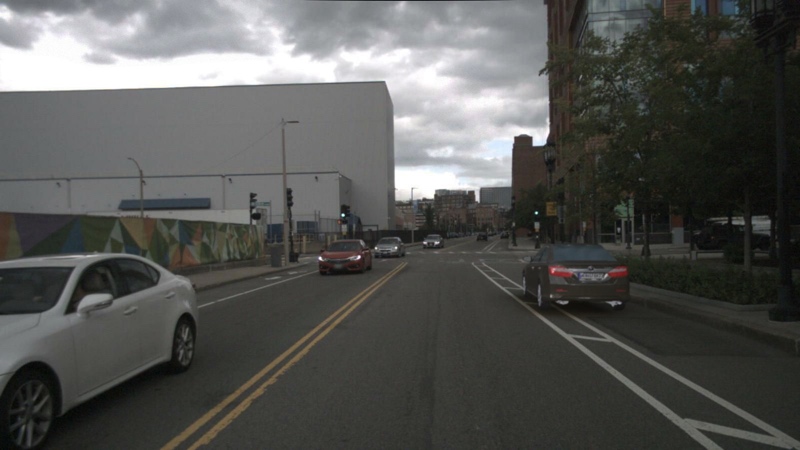
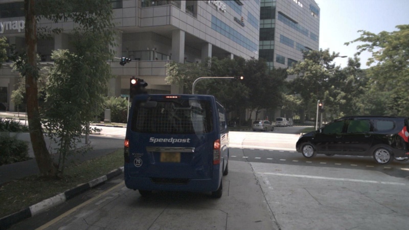
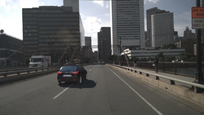
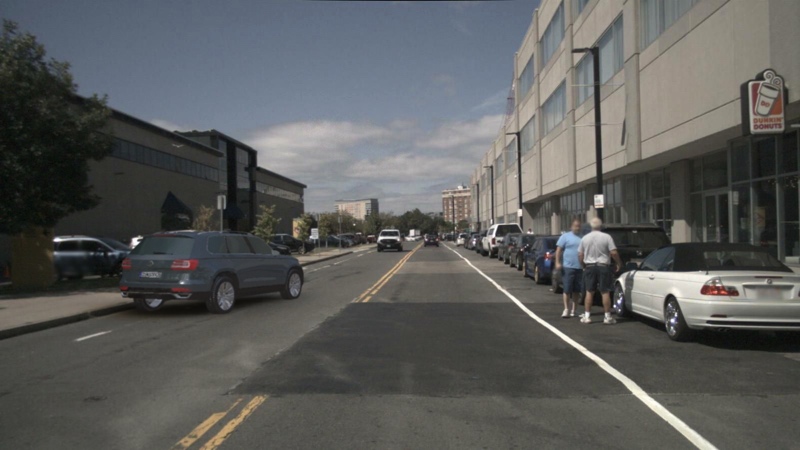
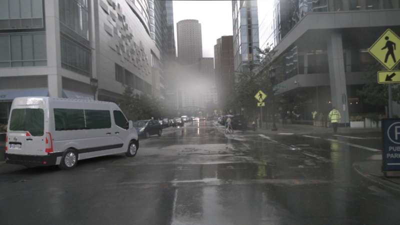
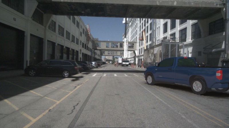
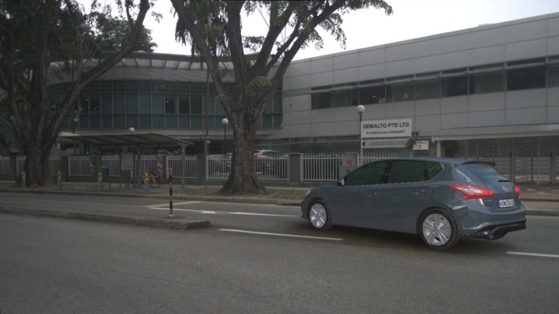
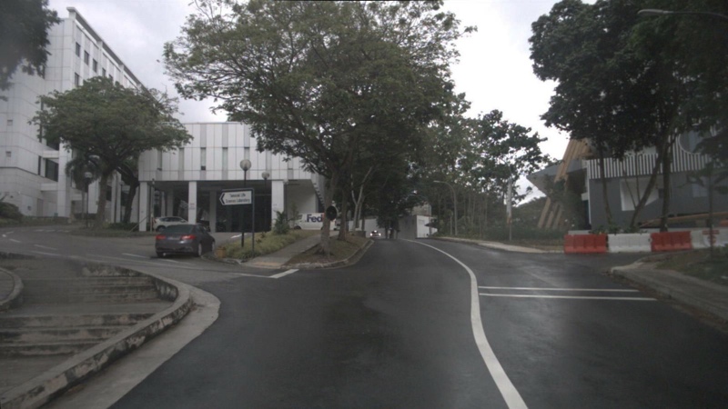
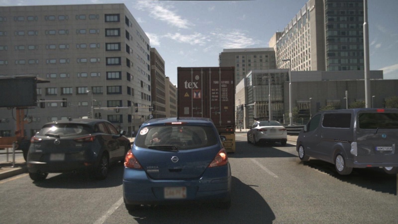
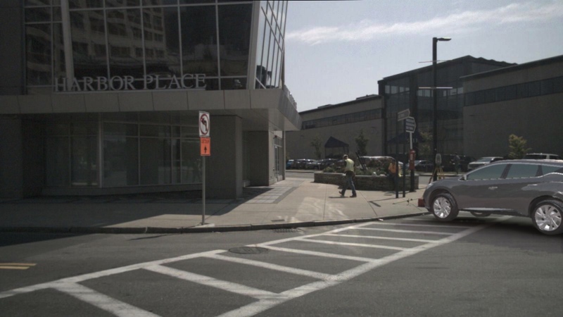
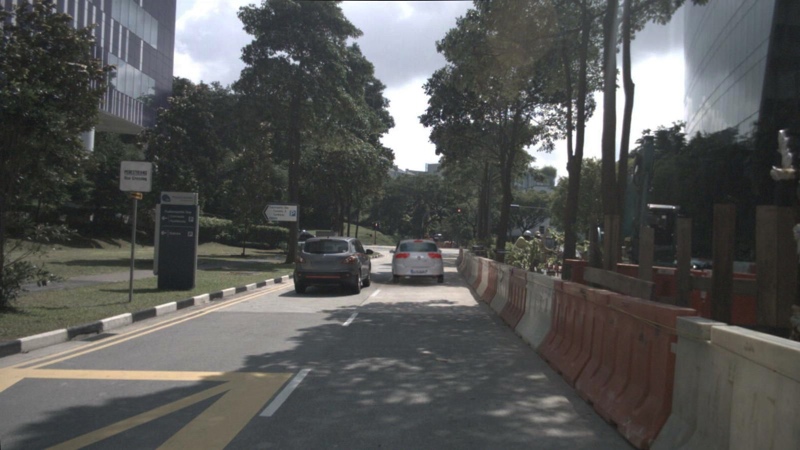
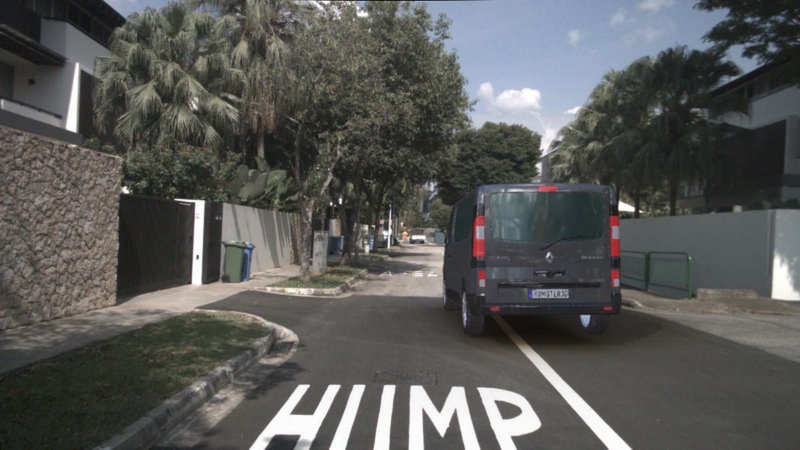
Figure J: Qualitative results of automatic data augmentation on nuScenes dataset [2]. Each image contains one inserted virtual car rendered with our neural AR approach.

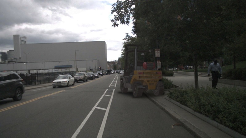
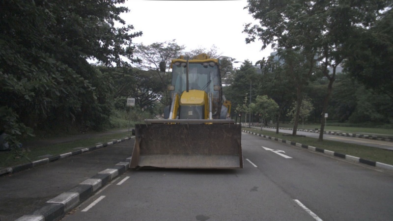
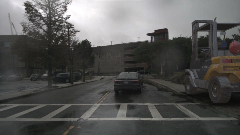
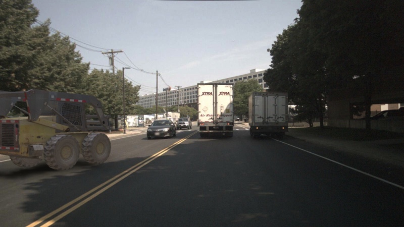
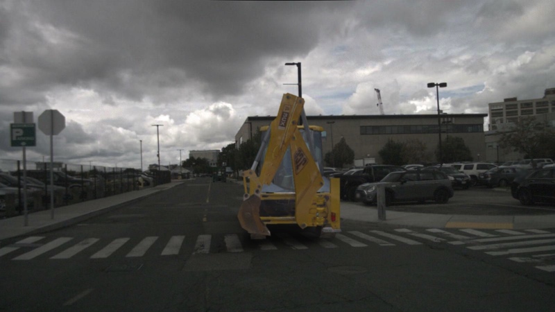
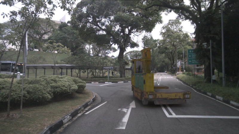
Figure K: Construction vehicle insertion results of automatic data augmentation on nuScenes dataset [2]. Our neural AR approach is agnostic to the category of 3D assets and can realistically insert virtual objects belonging to rare classes.

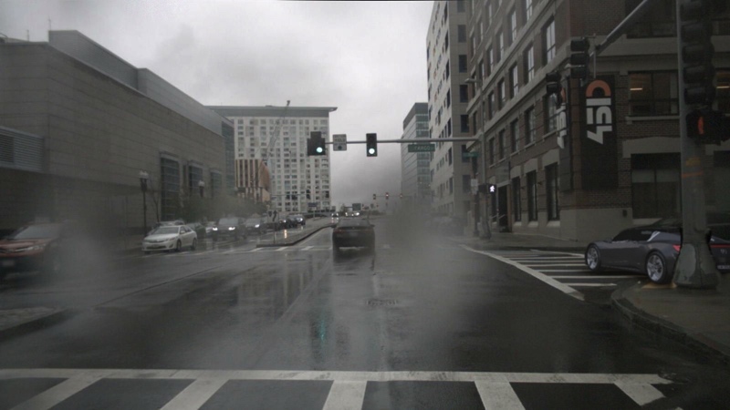
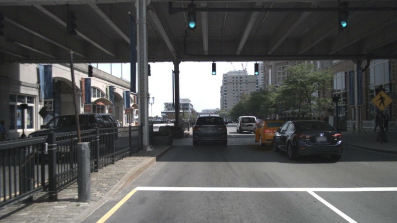
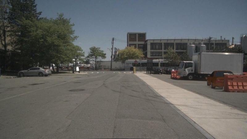
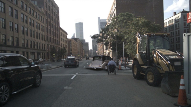
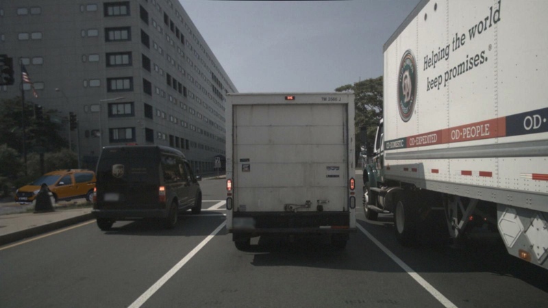
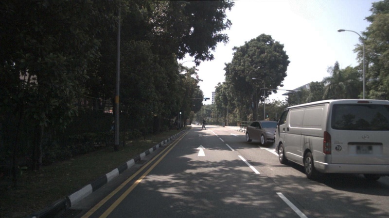
Figure L: Occlusion results of automatic data augmentation on nuScenes [2]. We naively handle occlusion by comparing the scene depth map and object Z buffer. Scene depth map is predicted with a pre-trained state-of-the-art monocular depth estimation model PackNet [7].

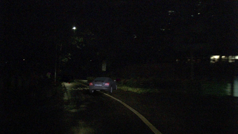
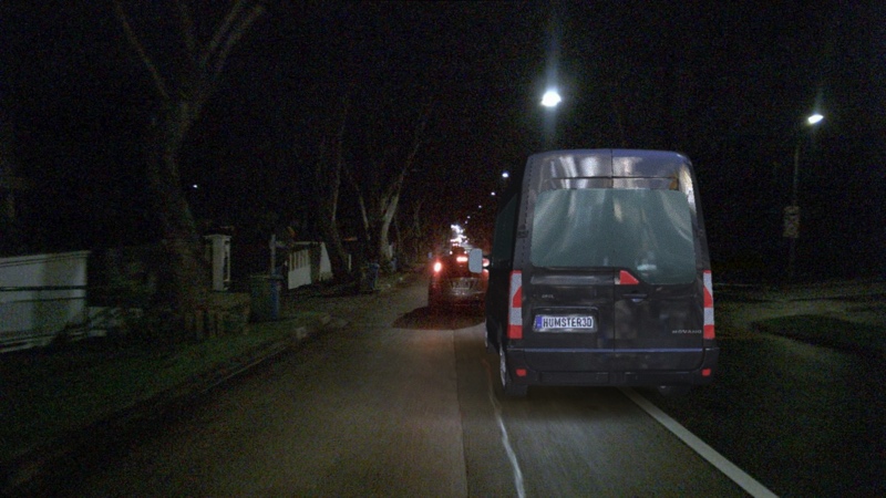
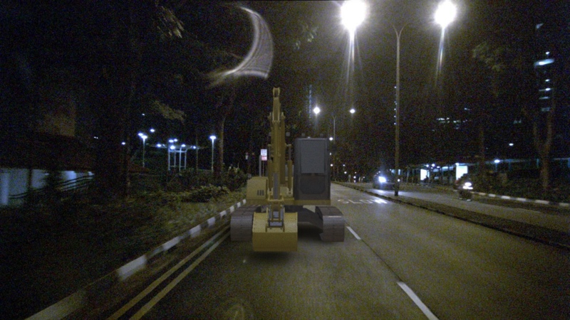
Figure M: Night time results of automatic data augmentation on the nuScenes dataset [2]. Our method can produce reasonable results without any HDR data supervision for the night time outdoor scenes.

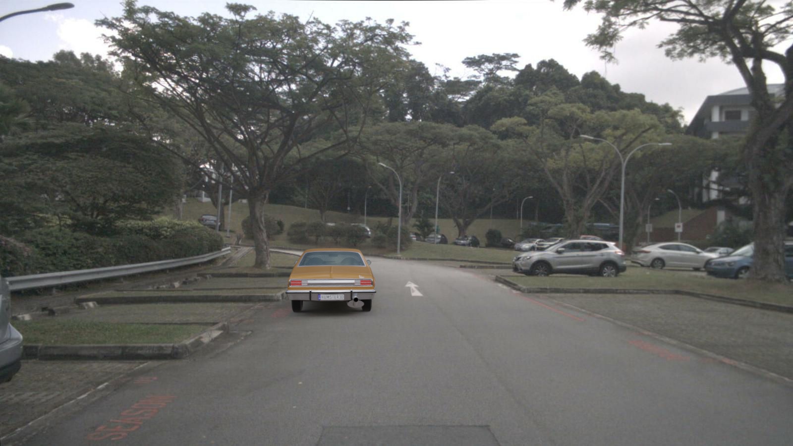
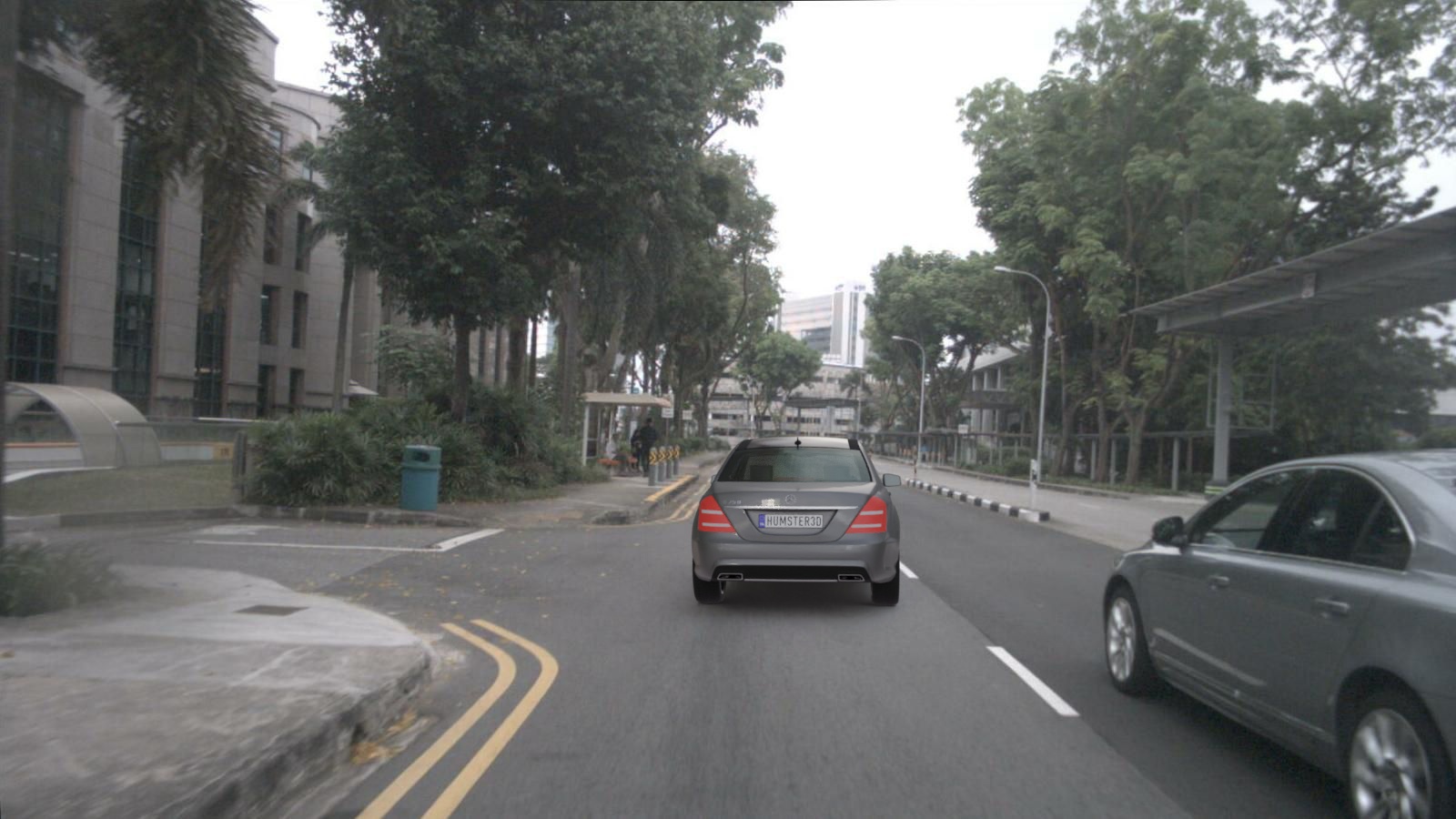
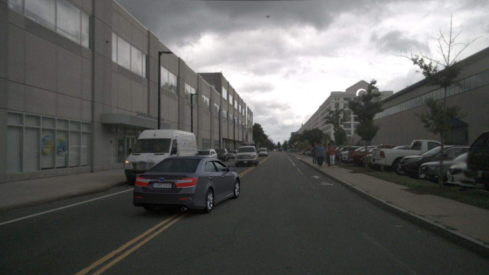
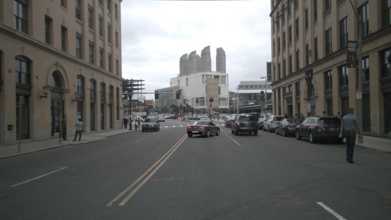
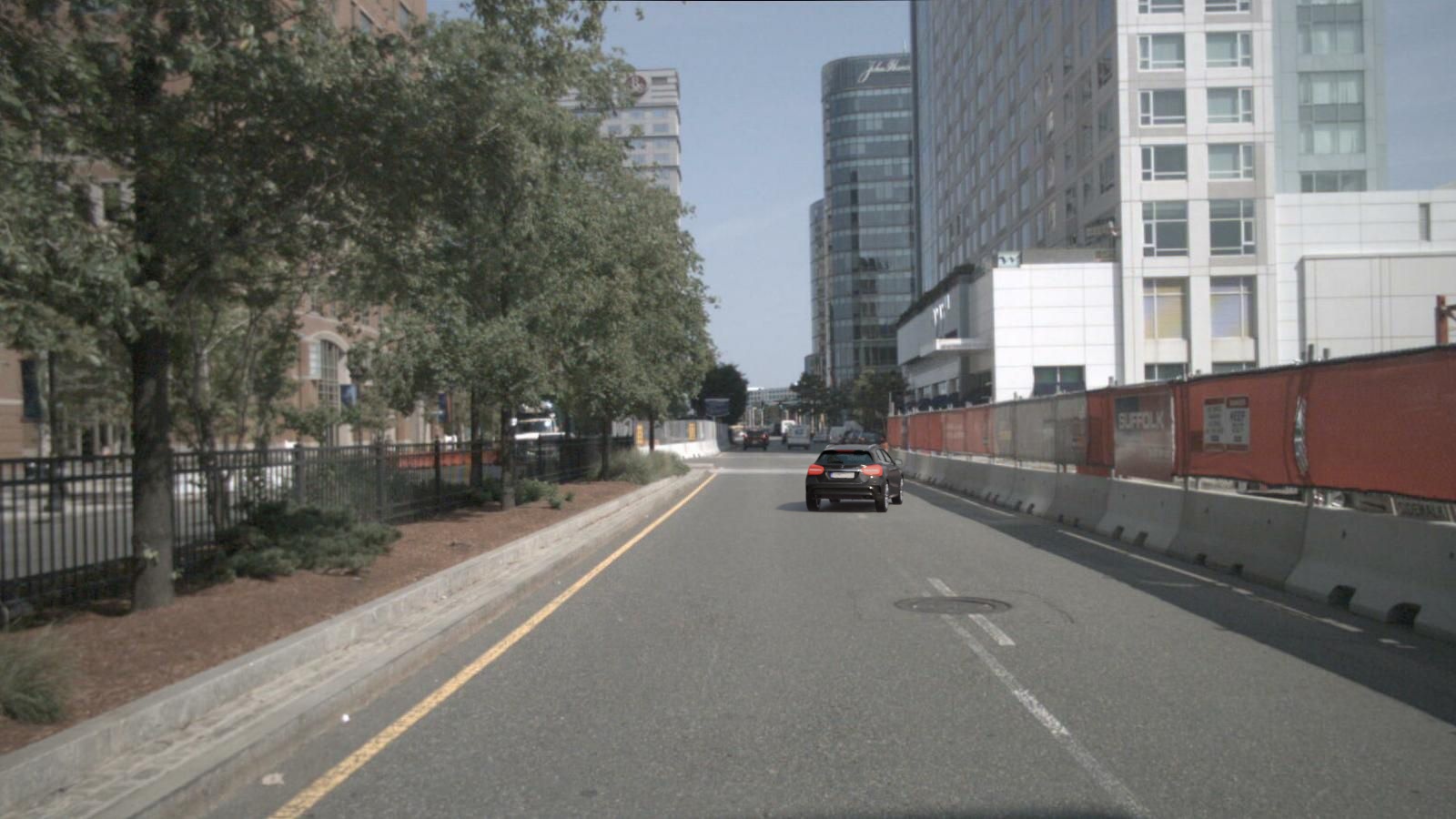
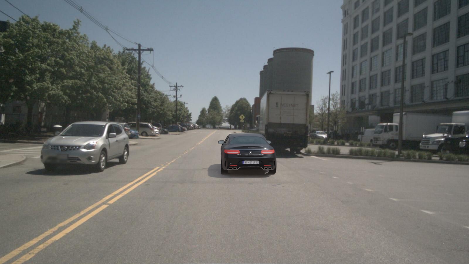
Figure N: Qualitative results of object insertion rendered by Blender. Our lighting representation can be rendered into location-specific environment map, which is compatible with commercial renderers. Integrated with powerful rendering engines, our method can leverage complex materials such as transparency and multi-bounce ray-tracing.

Initial editing results	5 iterations	10 iterations

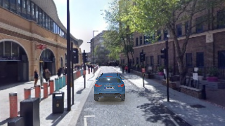
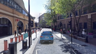
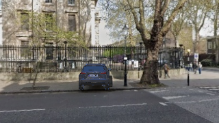
Figure O: Qualitative visualization of the test-time optimization. To understand the behaviour of the discriminator, we perform test-time optimization for the network parameters, where the only objective is to minimize the discriminator loss $\mathcal{L}_{\text{adv}}$. On the first column, we display the 320x180 resolution image editing results, which are consumed by the discriminator. The second and the third column shows the image editing results after 5 and 10 iterations. Note how the discriminator corrects the shadow direction in the first row, and removes obvious erroneous highlight in the second row. (Best viewed zooming in. We refer to additional animated result in the accompanied video.)

(a) Sensor effects	(b) Non-Lambertian shadows	(c) Occlusion

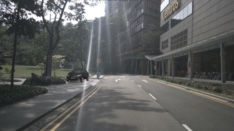
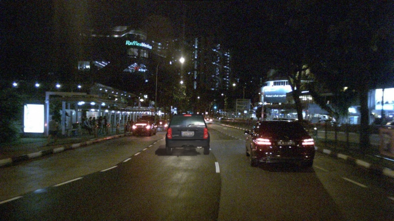
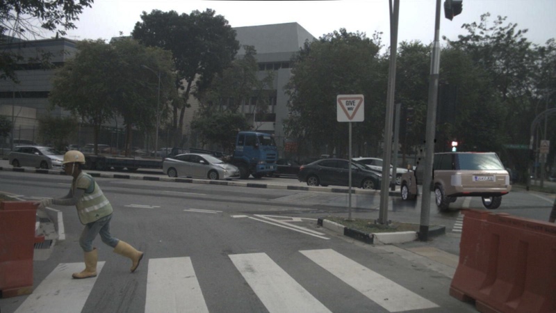
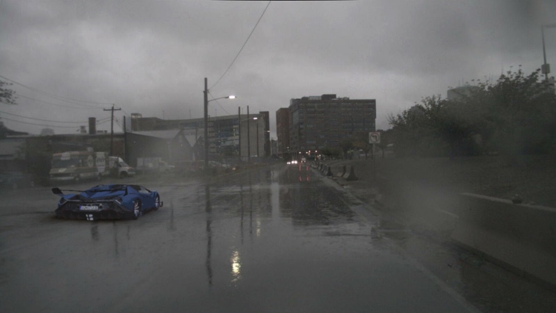
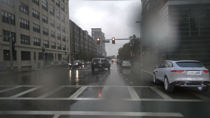
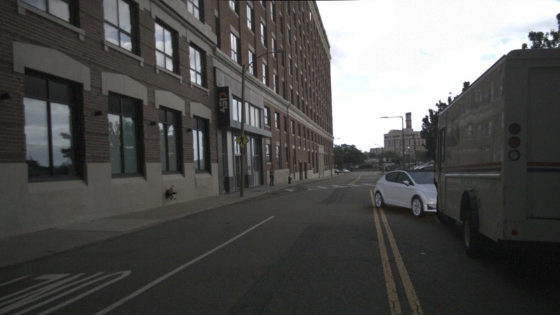
Figure P: Qualitative results – failure cases. (a) The virtually inserted object may not pass exactly the same environment and signal processing pipeline as the real-world captured scene pixels, e.g. the virtual object cannot reconstruct the halo effects of the sun and blurry regions caused by rain drops on the camera. (b) We assume a Lambertian scene surface when rendering the shadows, and thus the quality of editing results may decrease for wet specular road surfaces on rainy days. (c) Our occlusion handling relies on depth ordering, and may generate artifacts when the scene depth map prediction is inaccurate.

References

- [1] Burley, B., Studios, W.D.A.: Physically-based shading at disney. In: ACM SIGGRAPH. vol. 2012, pp. 1–7. vol. 2012 (2012)
- [2] Caesar, H., Bankiti, V., Lang, A.H., Vora, S., Liong, V.E., Xu, Q., Krishnan, A., Pan, Y., Baldan, G., Beijbom, O.: nuscenes: A multimodal dataset for autonomous driving. arXiv preprint arXiv:1903.11027 (2019)
- [3] Chen, W., Litalien, J., Gao, J., Wang, Z., Tsang, C.F., Khalis, S., Litany, O., Fidler, S.: DIB-R++: Learning to predict lighting and material with a hybrid differentiable renderer. In: Advances in Neural Information Processing Systems (NeurIPS) (2021)
- [4] Chen, Y., Rong, F., Duggal, S., Wang, S., Yan, X., Manivasagam, S., Xue, S., Yumer, E., Urtasun, R.: Geosim: Realistic video simulation via geometry-aware composition for self-driving. In: CVPR (2021)
- [5] Community, B.O.: Blender - a 3D modelling and rendering package. Blender Foundation, Stichting Blender Foundation, Amsterdam (2018), http://www.blender.org
- [6] González, Á.: Measurement of areas on a sphere using fibonacci and latitude–longitude lattices. Mathematical Geosciences 42(1), 49–64 (2010)
- [7] Guizilini, V., Ambrus, R., Pillai, S., Raventos, A., Gaidon, A.: 3d packing for self-supervised monocular depth estimation. In: IEEE Conference on Computer Vision and Pattern Recognition (CVPR) (2020)
- [8] He, K., Zhang, X., Ren, S., Sun, J.: Deep residual learning for image recognition. CoRR abs/1512.03385 (2015), http://arxiv.org/abs/1512.03385
- [9] Hold-Geoffroy, Y., Athawale, A., Lalonde, J.F.: Deep sky modeling for single image outdoor lighting estimation. In: Proceedings of the IEEE/CVF Conference on Computer Vision and Pattern Recognition. pp. 6927–6935 (2019)
- [10] Hold-Geoffroy, Y., Sunkavalli, K., Hadap, S., Gambaretto, E., Lalonde, J.F.: Deep outdoor illumination estimation. In: Proceedings of the IEEE Conference on Computer Vision and Pattern Recognition. pp. 7312–7321 (2017)
- [11] Isola, P., Zhu, J.Y., Zhou, T., Efros, A.A.: Image-to-image translation with conditional adversarial networks. CVPR (2017)
- [12] Karis, B., Games, E.: Real shading in unreal engine 4. Proc. Physically Based Shading Theory Practice 4(3) (2013)
- [13] Kingma, D.P., Ba, J.: Adam: A method for stochastic optimization (2017)
- [14] Li, Z., Shafiei, M., Ramamoorthi, R., Sunkavalli, K., Chandraker, M.: Inverse rendering for complex indoor scenes: Shape, spatially-varying lighting and svbrdf from a single image. In: Proceedings of the IEEE/CVF Conference on Computer Vision and Pattern Recognition. pp. 2475–2484 (2020)
- [15] Long, J., Shelhamer, E., Darrell, T.: Fully convolutional networks for semantic segmentation. In: Proceedings of the IEEE conference on computer vision and pattern recognition. pp. 3431–3440 (2015)
- [16] Mescheder, L., Oechsle, M., Niemeyer, M., Nowozin, S., Geiger, A.: Occupancy networks: Learning 3d reconstruction in function space. In: Proceedings of the IEEE Conference on Computer Vision and Pattern Recognition. pp. 4460–4470 (2019)
- [17] Ost, J., Mannan, F., Thuerey, N., Knodt, J., Heide, F.: Neural scene graphs for dynamic scenes. In: Proceedings of the IEEE/CVF Conference on Computer Vision and Pattern Recognition (CVPR). pp. 2856–2865 (June 2021)
- [18] Park, T., Liu, M.Y., Wang, T.C., Zhu, J.Y.: Semantic image synthesis with spatially-adaptive normalization. In: Proceedings of the IEEE Conference on Computer Vision and Pattern Recognition (2019)
- [19] Sengupta, S., Gu, J., Kim, K., Liu, G., Jacobs, D.W., Kautz, J.: Neural inverse rendering of an indoor scene from a single image. In: International Conference on Computer Vision (ICCV) (2019)
- [20] Wang, Z., Philion, J., Fidler, S., Kautz, J.: Learning indoor inverse rendering with 3d spatially-varying lighting. In: Proceedings of International Conference on Computer Vision (ICCV) (2021)
- [21] Zhang, J., Sunkavalli, K., Hold-Geoffroy, Y., Hadap, S., Eisenman, J., Lalonde, J.F.: All-weather deep outdoor lighting estimation. In: Proceedings of the IEEE Conference on Computer Vision and Pattern Recognition. pp. 10158–10166 (2019)
- [22] Zhou, Y., Huang, J., Dai, X., Luo, L., Chen, Z., Ma, Y.: HoliCity: A city-scale data platform for learning holistic 3D structures (2020), arXiv:2008.03286 [cs.CV]