GJ 1252b: A Hot Terrestrial Super-Earth With No Atmosphere

Abstract

In recent years the discovery of increasing numbers of rocky, terrestrial exoplanets orbiting nearby stars has drawn increased attention to the possibility of studying these planets’ atmospheric and surface properties. This is especially true for planets orbiting M dwarfs, whose properties can best be studied with existing observatories. In particular, the minerological composition of these planets and the extent to which they can retain their atmospheres in the face of intense stellar irradiation both remain unresolved. Here we report the detection of the secondary eclipse of the terrestrial exoplanet GJ 1252b, obtained via ten eclipse observations using the Spitzer Space Telescope’s IRAC2 4.5 µm channel. We measure an eclipse depth of 0pt${}^{+25}_{-32}$ ppm, corresponding to a day-side brightness temperature of 1410${}^{+91}_{-125}$ K. This measurement is consistent with the prediction for a bare rock surface. Comparing the eclipse measurement to a large suite of simulated planetary spectra indicates that GJ 1252b has a surface pressure of $\lesssim 10$ bar — i.e., substantially thinner than the atmosphere of Venus. Assuming energy-limited escape, even a 100 bar atmosphere would be lost in $<$1 Myr, far shorter than our gyrochronological age estimate of 3.9$\pm$0.4 Gyr. The expected mass loss could be overcome by mantle outgassing, but only if the mantle’s carbon content were $>$7% by mass — over two orders of magnitude greater than that found in Earth. We therefore conclude that GJ 1252b has no significant atmosphere. Model spectra with granitoid or feldspathic surface composition, but with no atmosphere, are disfavored at $>$2$\sigma$. The eclipse occurs just +1.4${}^{+2.8}_{-1.0}$ min after orbital phase 0.5, indicating $e\cos\omega$=+0.0025${}^{+0.0049}_{-0.0018}$, consistent with a circular orbit. Tidal heating is therefore likely to be negligible to GJ 1252b’s global energy budget. Finally, we also analyze additional, unpublished TESS transit photometry of GJ 1252b which improves the precision of the transit ephemeris by a factor of ten, provides a more precise planetary radius of 1.180$\pm$0.078 $R_{\oplus}$, and rules out any transit timing variations with amplitudes $\gtrsim 1$ min.

1 Introduction

Rocky planets on short-period orbits are among the most common planetary bodies known to emerge from the process of star and planet formation (e.g., Fulton & Petigura, 2018). Though too small to retain a primordial hydrogen envelope, such planets may produce secondary atmospheres later in their evolution. For example, in the Solar System, rocky bodies exhibit a wide diversity of atmospheric surface pressures from Venus (92 bar) to Earth and Titan ($\sim$1 bar) to Mars (6 mbar) to Mercury and the Moon (negligible atmospheres).

The conditions under which terrestrial planets can retain sizable atmospheres under different irradiation levels, timescales, types of host star, and planet masses, radii, and surface gravity all remain areas of active research. While an exoplanet’s atmosphere can be studied via transit and/or eclipse observations, transmission spectroscopy has so far failed to conclusively determine the properties (or absence of) any rocky planet’s atmosphere (e.g., see Wordsworth & Kreidberg, 2021). To date, emission measurements have offered the best prospects for studying the properties of terrestrial exoplanets.

Secondary eclipses of several rocky planets were detected at optical wavelengths by the Kepler/K2 missions (e.g., Batalha et al., 2011; Sheets & Deming, 2014; Malavolta et al., 2018). Unfortunately, such measurements often suffer from a degeneracy: optical eclipses represent a combination of reflected/scattered light and thermal emission, with no empirical way to determine the relative contributions of each.

Until now thermal infrared radiation has been measured from only two terrestrial exoplanets, LHS 3844b (Kreidberg et al., 2019) and K2-141b (Zieba et al., 2022). Spitzer 4.5 µm observations of these planets’ eclipse and phase curves revealed no phase offset and suggested an upper limit to the atmospheric surface pressure; for example, the data set for LHS 3844b indicates $P_{\mathrm{surf}}\lesssim 10$ bar.

In this paper we report 4.5 µm eclipse photometry that reveals thermal emission, and similar constraints on the atmosphere, of GJ 1252b, the smallest exoplanet for which such a measurement has been made to date. The planet has an Emission Spectroscopy Metric (ESM; Kempton et al., 2018) of 17, slightly larger than that of K2-141b and a factor of two smaller than LHS 3844b. GJ 1252b was identified by the TESS project as TESS Object of Interest (TOI) 1078.01 in data from Sector 13, the last southern sector to be observed in the first year of TESS operations. Shporer et al. (2020) confirmed the planetary nature of the signal using a combination of TESS photometry and HARPS radial velocities. They reported a planet orbiting an M3V star with radius of $1.193\pm 0.074\,R_{\oplus}$, and the planet’s mass is $1.32\pm 0.28\,M_{\oplus}$ (Luque et al., in review).

In Sec. 2 we present our TESS and Spitzer observations and our analyses of these data. Sec. 3 then discusses these measurements in light of a set of models of planetary spectra, leading us to conclude that any atmosphere on GJ 1252b likely has a surface pressure of $\lesssim$10 bar. Sec. 4 presents our predictions for atmospheric escape from GJ 1252b, which leads us to conclude that even an atmosphere with surface pressure $>$10 bar would be lost on a timescale much shorter than the system age. Finally, we close with a discussion of GJ 1252b in the context of similar measurements of other rocky exoplanets in Sec. 5.

2 Observations

2.1 New TESS Transit Photometry

Subsequent to the mid-2019 TESS Sector 13 photometry used to first discover GJ 1252b (Shporer et al., 2020), the system was re-observed during the TESS Sector 27 Campaign using Camera 2 from 2020 July 5 to 2020 July 30. In this section we describe our combined analysis of both the original Sector 13 and the new Sector 27 data. By performing a global fit on data sets separated by nearly a year, we further refine the orbital and planetary properties of GJ 1252b.

We downloaded both Sector 13 and 27 Presearch Data Conditioning (PDC) time series measurements from MAST. PDC-level data products are corrected for instrumental systematics and contamination from nearby stars. Our analysis used the LightKurve package (Lightkurve Collaboration et al., 2018) to perform 5 iterations of $3\sigma$ outlier rejection on data points above the median flux level. This removed 0.2% of data from the lightcurve. To remove any remaining flux variations we flattened the lightcurve using a Savitzky-Golay filter (Savitzky & Golay, 1964) after first masking out the transits (with one transit duration on either side) before applying the filter to ensure the transit features are not affected.

We fit the flattened lightcurve using the exoplanet package (Foreman-Mackey et al., 2021) which uses a Hamiltonian Monte Carlo (HMC) routine to explore the posterior probability distribution. Assuming a circular orbit with the period ($P$), time of inferior conjunction ($T_{0}$), scaled planet radius ($R_{P}/R_{*}$), impact parameter ($b$), transit duration ($T_{14}$), and mean flux offset ($\mu$) as free parameters we minimized a negative log-likelihood function. Our analysis held quadratic limb-darkening coefficients constant at $u_{0}$=0.2800 and $u_{1}$=0.3683 (values taken from Claret, 2017). We used the values obtained from the minimizer as initial positions for 32 parallel chains and ran the HMC for 2,000 tuning steps and 4,000 sampling steps per chain. Loose Gaussian priors (much wider than the final posteriors) were placed on $P$ (mean 0.51 days, width $\sigma$ 0.05 days) and $T_{\mathrm{conj}}$ (mean 1668.0, width 0.1) to prevent the sampler from wandering too far astray. The final Gelman-Rubin statistic of the HMC runs were $<1.01$ for all parameters.

The median values and their 1-$\sigma$ uncertainties are listed in Table 1, and the model fit to binned TESS data is shown in Figure 1. Our results agree well with those of the original discovery paper (Shporer et al., 2020). As an independent check, we also analyzed the full, two-sector TESS data set using the transit light curve code described in numerous similar K2 studies (e.g., Crossfield et al., 2015, 2016) and found consistent parameters in all cases.

We analyze only the transits because the current TESS data cannot usefully constrain the planet’s eclipse depth. In the TESS bandpass the contribution from either thermal emission (Fig. 6) or reflected light (Sec. 3.2.1) is $\lesssim$15 ppm, significantly smaller than our TESS transit depth precision of 61 ppm (Table 1).

Finally, we also performed a search for transit-timing variations (TTVs) in the TESS data, again using the exoplanet package. If present, TTV signals could indicate the presence of undiscovered companions due to mutual gravitational interactions or orbital decay due to tidal effects. Although the S/N of individual transit events is quite low, we find no evidence for TTVs with amplitudes $\gtrsim 1$ min, consistent with a lack of strongly perturbing companions. The deviation of GJ 1252b’s individually-measured transit times is consistent with a linear ephemeris across both sectors of TESS data. With nearly a year separating these two Sectors of TESS data, our analysis reduces the uncertainty on the period by an order of magnitude (see Table 1).

Table 1: Planet Parameters

Parameter	Units	Value	Source
Stellar parameters:
$R_{*}$	$R_{\odot}$	$0.391\pm 0.020$	Shporer et al. (2020)
$M_{*}$	$M_{\odot}$	$0.381\pm 0.019$	Shporer et al. (2020)
$T_{\mathrm{eff}}$	K	$3458\pm 137$	Shporer et al. (2020)
age	Gyr	3.9$\pm$0.4	This work, derived
TESS Transit parameters:
$T_{0}$	$BJD_{TDB}$	$2458668.09748\pm 0.00032$	This work, fit
$P$	d	$0.51824160\pm{0.00000069}$	This work, fit
$i$	deg	$84.8\pm 3.2$	This work, derived
$R_{P}/R_{*}$	–	$0.0277\pm 0.0011$	This work, fit
$a/R_{*}$	–	$5.03\pm 0.27$	This work, derived
$T_{14}$	hr	$0.724\pm 0.013$	This work, fit
$b$	–	$0.42\pm 0.24$	This work, fit
$a$	AU	$0.00915^{+0.00015}_{-0.00015}$	This work, derived
$S_{inc}$	$S_{\oplus}$	$233^{+48}_{-41}$	This work, derived
$R_{P}$	$R_{\oplus}$	1.180$\pm$0.078	This work, derived
$M_{P}$	$M_{\oplus}$	$1.32\pm 0.28$	Luque et al., in review
Spitzer Eclipse parameters:
$T_{E}$	$BJD_{TDB}$	2458668.3575${}^{+0.0019}_{-0.0007}$	This work, fit
$\delta_{IRAC2}$	ppm	0pt${}^{+25}_{-32}$	This work, fit
$dt$	min	+1.4${}^{+2.8}_{-1.0}$	This work, derived
$e\cos\omega$	–	+0.0025${}^{+0.0049}_{-0.0018}$	This work, derived
$T_{\mathrm{day}}$	K	1410${}^{+91}_{-125}$	This work, derived
$f$	–	$>$0.40	This work, derived
$A_{B}$	–	$<$0.41	This work, derived
$f\left(1-A_{B}\right)$	–	$>$0.37	This work, derived

Table 2: Spitzer/IRAC 4.5 µm Observations

	Start Date	Start	End	$\delta$	$\sigma_{\delta}$
AOR	[$BJD_{TDB}$]	Phase	Phase	[ppm]	[ppm]
71407360	2458868.859948	0.3917	0.6228	86	88
71407872	2458867.834249	0.4125	0.6436	101	97
71408384	2458866.277380	0.4084	0.6395	$-$4	88
71408640	2458864.190715	0.3819	0.6131	168	83
71408896	2458863.686588	0.4092	0.6403	44	87
71409152	2458863.163738	0.4003	0.6314	123	86
71409408	2458861.090252	0.3993	0.6304	221	83
71409664	2458860.062523	0.4162	0.6473	357	103
71409920	2458859.008577	0.3825	0.6136	307	88
71410176	2458869.902201	0.4028	0.6340	137	83

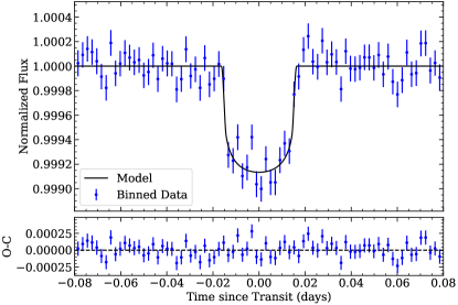
Figure 1: Folded and binned two-sector TESS lightcurve (blue points) with the median model plotted in black. Residuals (data minus model) are shown in the lower panel.

2.2 Spitzer Eclipse Photometry and Analysis

2.2.1 Eclipse Observations

Soon after the TESS project’s announcement of a planet candidate around GJ 1252, and before the planet’s confirmation by Shporer et al. (2020), we identified the planet candidate as a promising target for thermal infrared emission measurements obtained during secondary eclipse. Using preliminary information provided in the TESS alert and the TESS Input Catalog (TIC; Stassun et al., 2018), we estimated that a coordinated campaign of Spitzer eclipse observations could detect the planet’s eclipses. We therefore scheduled ten 4.5 µm eclipse observations as part of Spitzer Program 14084 (Crossfield et al., 2018).

We observed the ten eclipses of GJ 1252b over ten days in January 2020. The final observations were taken on UT 2020-01-21, less than ten days before Spitzer was deactivated on 2020-01-30. Each eclipse observation was an identical, 2.9 hr, continuous, staring observation centered on the predicted time of secondary eclipse (i.e., orbital phase 0.5). The visits consisted of 5120 subarray frames with 2 s integrations, taken with the IRAC2 4.5 µm camera (Fazio et al., 2004). The observations used IRAC’s peak-up mode to place the star near a well-characterized and well-behaved region of the detector, in order to minimize the effect of IRAC’s well-known intrapixel sensitivity variations. Table 2 lists the times and orbital phases of each of the ten eclipse observations.

2.2.2 Eclipse Analysis

We analyzed the Spitzer photometry using Pixel-Level Decorrelation (PLD; Deming et al., 2015), which models the systematics-dominated Spitzer light curve as a linear combination of basis vectors derived from each pixel’s time series. Specifically, we use the formulation

$$f_{ik}=\left(\sum_{j=1}^{N+M}c_{jk}v_{ijk}\right)m_{ik}$$ (1)

where $f_{ik}$ is the modeled flux at the $i^{\mathrm{th}}$ timestep of the $k^{\mathrm{th}}$ eclipse visit, $c_{jk}$ is the scaling coefficient for the corresponding basis vector $v_{ijk}$, and $m_{ik}$ is the purely astrophysical model of a secondary eclipse. The basis vectors $v_{ijk}$ always include the $N$ individual pixel time series from the $k^{\mathrm{th}}$ visit (the “pixel-level” data essential to PLD) and may also include $M$ low-order temporal trends (for which $v_{ijk}=t_{ijk}^{p}$ for $p=0,1,...(M-1)$ ) or other systematic vectors against which the data will be decorrelated. In our analysis we included a linear trend with time in order to remove a slow, long-term drift. We parameterized the eclipse model ($m_{ik}$) using the Mandel & Agol (2002) formulae for the occultation of an object with uniform surface brightness, with its only free parameters being the time of mid-eclipse $T_{E}$ and the fractional eclipse depth $\delta$.

PLD is often applied by simultaneously sampling the posterior distribution of the nuisance parameters $c_{jk}$ as well as the astrophysical parameters of interest. In our case, this turned out to be intractable. With ten eclipse visits, the use of $N=9$ pixels and $M=1$ (constant scaling, linear polynomial trend) would require marginalizing over 100 nuisance parameters to obtain measurements of just two astrophysical parameters, $T_{E}$ and $\delta$.

Instead, we determine $T_{E}$ and $\delta$, and their uncertainties, as follows. For each combination of these parameters, we calculate a model eclipse light curve and divide the observed flux $F_{ik}$ by it. The result is

$$\frac{F_{ik}}{m_{ik}}\approx\sum_{j=1}^{N+M}c_{jk}v_{ijk}+\epsilon_{ik}$$ (2)

where $\epsilon_{ik}$ represent the measurement errors. We then directly solve Eq. 2 at each point for the $c_{jk}$ using weighted linear least squares. This approach allows us to directly sample the two-dimensional $(T_{E},\delta)$ plane while also accounting for the interrelationships of these astrophysical parameters on the $c_{jk}$ nuisance parameters. This approach is similar in some ways to the PLD analysis of Spitzer/IRAC microlensing observations (Dang et al., 2020); the main difference is that that work had more than two astrophysical parameters of interest and so used MCMC sampling instead of directly calculating a grid of likelihood values.

We set the weight of each observation equal to $1/\sigma^{2}$, where $\sigma$ is the 68.3% central confidence interval on the dispersion of the residuals to an initial fit. Flux measurements $F_{ik}$ are set to zero weight if they deviate by more than $5\sigma$ from the nominal model.

The resulting stacked, detrended eclipse light curve shown in Fig. 2 shows a clear flux decrement of 0pt${}^{+25}_{-32}$ ppm at the expected time of eclipse. Our measured eclipse parameters are listed in Table 1, while the light curves for each individual visit, as well as Allan deviation plots of the residuals to each visit, are shown in the Appendix. As two checks on our measured eclipse depth, we also calculated the weighted mean of the eclipse depths from each individual visit, and also conducted a joint analysis in which the time of eclipse was held fixed to orbital phase 0.5. The weighted mean is $150\pm 28$ ppm, while the fixed-time analysis yields a depth of $140^{+35}_{-20}$ ppm; both these values are consistent with the value obtained from our joint fit.

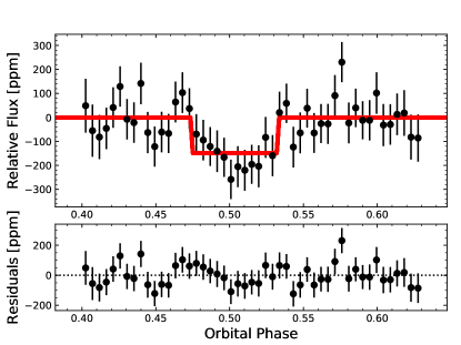
Figure 2: Spitzer 4.5 µm photometry and secondary eclipse fit (top) and residuals to the fit (bottom). The photometry is shown after detrending for systematic effects, combining the photometry from all ten eclipse visits, and binning down to a two-minute cadence. The measured depth is 0pt${}^{+25}_{-32}$ ppm.

2.3 Stellar Age From Gyrochronology

Finally, to interpret our measurements of GJ 1252b’s thermal emission and estimate its atmospheric evolution (described below), we need to estimate a stellar age. Inferring ages for mature, field M dwarfs is notoriously challenging; one promising avenue for all but the latest M spectral subtypes is the use of gyrochronology. Using the spindown analysis of Engle & Guinan (2018) together with GJ 1252’s stellar rotation period of $64\pm 4$ d (Shporer et al., 2020), we estimate GJ 1252’s age to be 3.9$\pm$0.4 Gyr. This indicates that GJ 1252 is somewhat younger than LHS 3844 (7.8$\pm$1.6 Gyr; Kane et al., 2020), an estimate broadly consistent with the non-detection of stellar flares during the first sector of TESS observations of GJ 1252 (Howard, 2022). This result also indicates that the GJ 1252 system is somewhat younger than the $7.8\pm 1.6$ Gyr LHS 3844b (Kane et al., 2020).

3 Timing, Tides, and Atmospheres

Our analysis of the Spitzer/IRAC2 4.5 µm photometry clearly detects the secondary eclipse signal, which has a depth of $\delta$=0pt${}^{+25}_{-32}$ ppm and a timing offset from orbital phase 0.5 of just +1.4${}^{+2.8}_{-1.0}$ min (the joint posterior distribution of eclipse depth and eclipse timing is shown in the Appendix). Here we discuss the implications of these measurements: first of the eclipse timing in Sec. 3.1, and then of the measured depth in Sec. 3.2

3.1 Eclipse Time and Implications

The offset of the eclipse time from orbital phase 0.5 constrains the combination of orbital parameters $e\cos\omega$ (Winn, 2010); for GJ 1252b we find $e\cos\omega$=+0.0025${}^{+0.0049}_{-0.0018}$. This result is consistent with zero at the 1.4$\sigma$ level, so we do not take this measurement as evidence of an eccentric orbit. Regardless, the $e\cos\omega$ measurement further justifies the assumption of low eccentricity in the radial velocity analysis of Shporer et al. (2020). We conducted a reanalysis of their radial velocity data while incorporating this new constraint on $e\cos\omega$, finding results consistent with those of the discovery paper.

Although GJ 1252b’s orbit would quickly circularize in the absence of other perturbers, small planets orbiting M dwarfs are often found in multi-planet systems and additional bodies in the system could cause GJ 1252b to stay on an eccentric orbit. Although no such bodies were indicated by our TTV analysis, it is still possible that tidal heating could act as an additional heat source in GJ 1252b. We estimate this heating level following the prescription of Henning et al. (2009) and assuming a Love number $k_{2}=0.3$ and tidal quality factor $Q=10^{4}$, approximately appropriate for super-Earths (Miguel et al., 2011; Millholland & Laughlin, 2019). Further assuming that $e=0.0025$, we find that tidal heating should contribute only $4\times 10^{16}$ W to GJ 1252b’s total energy budget, negligible (unless tidal heating is enhanced via a significantly nonzero axial tilt; Millholland & Laughlin, 2019) compared to the roughly $6\times 10^{19}$ W of starlight absorbed by the planet.

3.2 Eclipse Depth and Implications

Here we consider the implications of our eclipse measurement on the surface and atmospheric properties of GJ 1252b. We first consider our results in the context of global energy balance in Sec. 3.2.2, and then in the context of a suite of one-dimensional radiative transfer models in Sec. 3.2.3.

3.2.1 From Eclipse Depth to Brightness Temperature

Converting an eclipse depth measurement into a brightness temperature requires an estimate of both $R_{P}/R_{*}$ and of the stellar flux density at the relevant wavelengths. Since M dwarfs such as GJ 1252 have emergent spectra that differ considerably from simple blackbodies, appropriate stellar spectra must be used. We used the BT-Settl suite of stellar models (Allard, 2014), interpolating across the model grid using the $T_{\mathrm{eff}}$, $\log_{10}g$, and [Fe/H] from Shporer et al. (2020). The result is that GJ 1252b’s day side has a 4.5 µm brightness temperature of 1410${}^{+91}_{-125}$ K, considerably hotter than the equilibrium temperature of $1089\pm 69$ K reported by Shporer et al. (2020).

We note that reflection or scattered light contributes only $\left(R_{p}/a\right)^{2}A_{g}\approx\left(30\,\mathrm{ppm}\times A_{g}\right)$ to the eclipse depth, where $A_{g}$ is the planet’s 4.5 µm broadband geometric albedo. With $A_{g}<0.5$ expected for most typical minerals (Mansfield et al., 2019) and $<0.1$ for lava or volcanic glasses (Essack et al., 2020; Modirrousta-Galian et al., 2021), the contribution of surface reflection to our measurement is $<15$ ppm, smaller than our Spitzer (or TESS) measurement precision.

3.2.2 Energy Balance and Atmospheric Circulation

One phenomenological framework for interpreting single-band secondary eclipse measurements is to assume the planet radiates as a blackbody at the measured brightness temperature, then to use the measurement to constrain some combination of day-to-night heat redistribution parameter $f$ and Bond Albedo $A_{B}$ (e.g., Seager, 2010). In particular, the combination $f(1-A_{B})$ directly determines the planet’s day-side equilibrium temperature via

$$T_{\mathrm{eq}}=T_{\mathrm{eff}}\sqrt{\frac{R_{*}}{a}}\left(f\left[1-A_{B}\right]\right)^{1/4}.$$ (3)

In this formulation, the limiting values of $f$ are $\frac{2}{3}$, indicating no heat redistribution (e.g., consistent with no atmosphere) and $\frac{1}{4}$, indicating uniform heat redistribution around the planet. Fig. 3 shows our joint constraints on $f$ and $A_{B}$, assuming flat priors on both quantities and the system parameters listed in Table 1. In all cases the most likely values are the ones that give the highest day-side $T_{\mathrm{eq}}$, i.e. $f=\frac{2}{3}$ and $A_{B}=0$. We set upper limits (at 95.4%, or 2$\sigma$ confidence) of: a low albedo of $A_{B}<$ 0.41, a high redistribution parameter of $f>$ 0.40, and a high combination of the two, $f(1-A_{B})>$ 0.37.

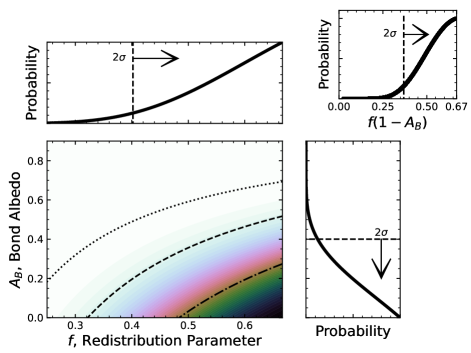
Figure 3: Joint constraints on Bond albedo and the heat redistribution parameter, assuming that GJ 1252b radiates as a blackbody at its 4.5 µm brightness temperature. More heavily shaded regions indicate higher probabilities in the main panel, with the contour lines demarcating the enclosed 1$\sigma$, 2$\sigma$, and $3\sigma$ confidence intervals. The dashed lines in the 1D posterior distribution plots show the 95.4% (2$\sigma$) confidence limit for the indicated parameter. Our measurements of GJ 1252b constrain $f>$ 0.40, $A_{B}<$ 0.41, and $f(1-A_{B})>$ 0.37.

3.2.3 One-dimensional Atmosphere Models

Finally, we also present a large suite of atmospheric models and spectra of GJ 1252b. These models are all available as machine-readable supplements to this paper. Our models and spectra are generated using the open-source, 1D radiative transfer code HELIOS (Malik et al., 2017, 2019b, 2019a), which simulates the planet in radiative-convective equilibrium and also provides the functionality to include the radiative effects of a non-gray surface on both the atmosphere and the planetary spectrum (see Whittaker et al., in prep.).

In HELIOS the temperature profile and surface temperature are obtained using the k-distribution method, with 420 wavelength bins (0.245 — 10⁵ $\mu$m). Then, starting from the equilibrium temperature profile, the planetary spectrum is calculated using opacity sampling with a resolution of $R$ = 4000. Convectively unstable atmospheric layers are corrected using convective adjustment. We model dayside-averaged conditions and use the scaling theory of Koll (2022) to estimate the amount of heat transported from the day-side to the night-side of the planet. In the bare-rock case, the heat redistribution parameter ($f$ in Eq. 3) is set to $2/3$, equivalent to no horizontal heat transport (Burrows et al., 2008; Hansen, 2008).

Gaseous opacities are calculated with HELIOS-K (Grimm & Heng, 2015; Grimm et al., 2021), including O₂ (Gordon et al., 2017), N₂(Gordon et al., 2022), H₂O (Polyansky et al., 2018), CO (Li et al., 2015), CO₂ (Rothman et al., 2010), CH₄ (Yurchenko et al., 2017) and SO₂ (Underwood et al., 2016). All opacities are calculated on a fixed grid with a resolution of 0.01 cm^-1, assuming a Voigt profile truncated at 100 cm^-1 from line center. For H₂O, CH₄ and SO₂ the default pressure broadening coefficients provided by the Exomol database are included. For O₂, N₂, CO and CO₂ the HITRAN broadening formalism for self-broadening is used. Further included are collision induced absorption (CIA) by O₂-O₂, O₂-CO₂, CO₂-CO₂, N₂-N₂, and N₂-CH₄ pairs (Richard et al., 2012) and Rayleigh scattering of H₂O, O₂, N₂, CO₂ and CO (Cox, 2000; Sneep & Ubachs, 2005; Wagner & Kretzschmar, 2008; Thalman et al., 2014).

To model the radiative effects of the surface, we use the geometric albedo spectra from Hu et al. (2012). For the bare-rock scenario, HELIOS again iterates the surface temperature until the surface is in radiative equilibrium, i.e., the downward stellar radiation equals the reflected plus emitted radiation at the surface boundary. This takes the non-gray surface albedo into account across the range of 0.3–25 µm, thus correctly treating both the stellar flux absorption and reflection as well as the planetary emission.

When modeling the planetary envelope we include the main infrared absorbers that may be plausibly found in secondary atmospheres — H₂O, CO₂, CO, CH₄, and SO₂ (see, e.g., Gillmann et al., 2022) — and vary their mixing ratios between 1 ppm and 1% (Gaillard & Scaillet, 2014). As background gas we use O₂ or N₂ (Wordsworth & Pierrehumbert, 2014; Luger & Barnes, 2015; Schaefer et al., 2016; Lammer et al., 2019). As limiting cases we also approximate post-water-runaway, Venus-like and carbon-rich (elemental C/O $\sim$ 1) atmospheres by adding pure H₂O, CO₂, and CO scenarios (Goldblatt, 2015; Kane et al., 2014; Madhusudhan, 2012). Specifically, the full range of our models included either CO or CH₄ in an N₂-dominated atmosphere; CO₂, SO₂, or H₂O in an O₂-dominated atmosphere; and atmospheres of pure CO₂, SO₂, or H₂O. These models are not intended to be exhaustive (nor may they all be chemically stable on geological timescales); our goal is to explore a representative range of atmospheres without overinterpreting our single-channel measurement.

For each model emission spectrum, we calculated the eclipse depth that would be measured in the 4.5 µm IRAC2 bandpass. Figs. 4 and 5 compare our measured 4.5 µm eclipse depths to the predictions of our atmospheric models dominated by N₂ and O₂, respectively. For the N₂-dominated models, Fig. 4 shows that the only models consistent with our eclipse measurement at 2$\sigma$ or better have $P_{\mathrm{surf}}\lesssim 1$ bar (for CO as the active IR absorber) and $\lesssim 10$ bar (for CH₄). Similarly, Fig. 5 shows that the O₂-dominated models consistent with our measurement at 2$\sigma$ have $P_{\mathrm{surf}}\lesssim 1$ bar (for CO₂) and $\lesssim 10$ bar (for SO₂ or H₂O).

We also find that models lacking any atmosphere are also consistent with our eclipse measurement. Fig. 6 shows that while only the gray and metal-rich bare-rock models are consistent with our measurement at $<$1$\sigma$, models with an oxidized Fe, basaltic, and ultramafic surface composition are all consistent with our eclipse at $<$2$\sigma$. Models with a feldspathic or granitoid surface composition are inconsistent with the data at $>$2$\sigma$. However, we note that the substellar region of GJ 1252b is likely hot enough for such materials to melt. Although our atmosphere-free models may not be strictly accurate for this planet’s surface, we leave more detailed models involving both solid and melted regions for future study.

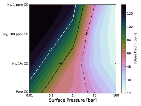
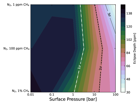
Figure 4: Predicted IRAC2 4.5 µm eclipse depths (colored shading) from our suite of atmospheric models for atmospheres dominated by N₂; each model has a single dominant, active IR absorber of either CO (top) or CH₄ (bottom). The contour lines indicate the level of agreement with our eclipse measurement of 0pt${}^{+25}_{-32}$, with darker regions being more consistent with our data. Thick atmospheres with $P_{\mathrm{surf}}\gtrsim 10$ bar are disfavored by all modeled mixing ratios.

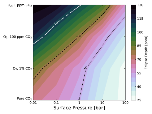
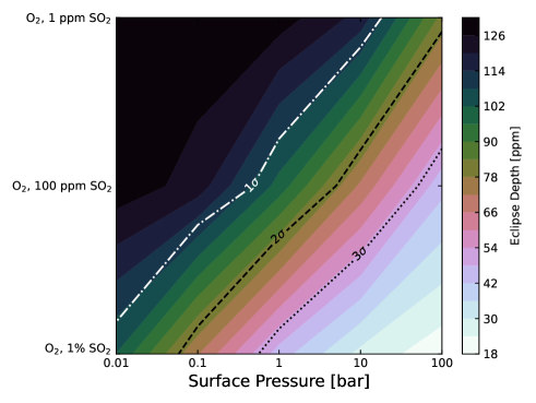
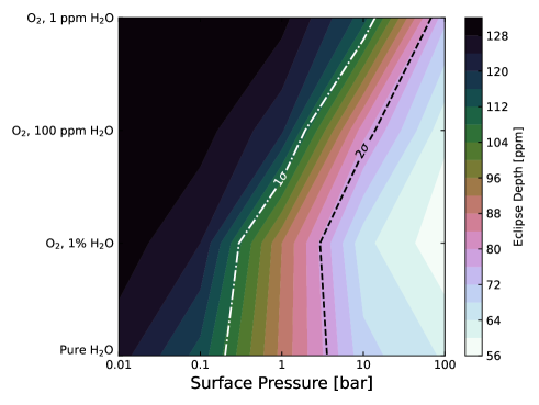
Figure 5: Same as Fig. 4 but for atmospheres dominated by O₂, and with active IR absorbers of CO₂ (top), SO₂ (middle), and H₂O (bottom). Thick atmospheres ($P_{\mathrm{surf}}\gtrsim 10$ bar) with mixing ratios of $\gtrsim 10^{-4}$ are disfavored in all cases.

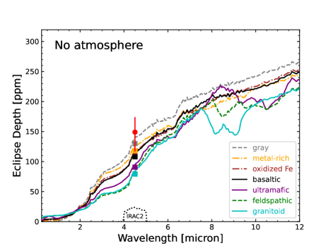
Figure 6: Simulated eclipse spectra of GJ 1252b from our suite of no-atmosphere models for different types of solid, unmelted surface mineralogies (lines; from Hu et al., 2012) compared to our measured depth and uncertainty (red circle with error bars). Squares show the values obtained by averaging the models over the IRAC2 bandpass (dotted line). All but the granitoid and feldspathic models are consistent with our measurement at $\leq$2$\sigma$.

4 Atmospheric Evolution and Escape

Zahnle & Catling (2017) postulate a “cosmic shoreline” in which the ability of a body to retain an atmosphere depends on some combination of its escape velocity $v_{\mathrm{esc}}$, bolometric irradiation $S$, and extreme UV (XUV) irradiation. Given its irradiation and $v_{\mathrm{esc}}$=5.4$\pm$0.8 m s^-1, GJ 1252b would lie well into the atmosphere-free zone — but then so would 55 Cnc e, where infrared measurements seem to indicate the presence of an atmosphere (Demory et al., 2016a; Tamburo et al., 2018; Demory et al., 2016b; Angelo & Hu, 2017; Hammond & Pierrehumbert, 2017). Thus the cosmic shoreline may not apply universally to smaller exoplanets irradiated so much more intensely than anything in the Solar System.

The evolution of a planetary atmosphere into its end-state depends on the mantle’s cooling rate, regions of oxidization, and potential sinks for these volatiles (e.g., Gillmann et al., 2022). For example, N₂ is interesting because there are relatively few sinks and so, despite N₂ being a relatively small amount of the Earth’s total volatile inventory, it dominates the present atmosphere. Another interesting species to think about is SO₂: the sulfur cycle on Venus is an important component of its overall atmospheric chemistry, and so SO₂ is a significant component of volcanic outgassing on Venus (Esposito, 1984; Korenaga, 2010; Zhang et al., 2012; Kane et al., 2019). Nonetheless SO₂ does not constitute nearly as much of the Venusian atmosphere as one might expect, largely because it reacts with calcium carbonates to produce CO (Hong & Fegley, 1997). Thus one possible end-state for a desiccated rocky planet’s atmosphere would be an atmosphere consisting of mainly CO₂, N₂, CO, CH₄, and SO₂. Any H₂O would remain through the moist greenhouse phase (if any), but would probably end up the same fate as past water on Venus: disassociation, loss of H₂, and oxidization of the surface and reaction with CH₄ to produce more CO₂ (Kane et al., 2020).

4.1 Energy-Limited Escape

We first estimate the atmospheric loss rate from GJ 1252b using the formalism of energy-limited atmospheric escape (Salz et al., 2016), leaving more involved estimates of the planet’s mass-loss rate for future work. Using the MUSCLES treasury survey’s spectra of nearby M dwarfs (France et al., 2016; Youngblood et al., 2016; Loyd et al., 2016) we estimate an XUV flux incident on GJ 1252b of $(6-8)\times 10^{3}$ erg s^-1 cm^-2. Assuming a heating efficiency of 0.3 (Salz et al., 2015) and that the planet’s optical transit radius is the same as its effective radius of XUV absorption, this XUV flux translates into an atmospheric mass loss rate of roughly $0.1M_{\oplus}$ Gyr^-1. The mass of a planet’s atmosphere is just $4\pi R_{p}^{2}P_{\mathrm{surf}}/g_{\mathrm{surf}}$, which for GJ 1252b is $\left(5.3\times 10^{18}\mathrm{~{}kg}\right)\left(P_{\mathrm{surf}}/\mathrm{1~{}bar}\right)$. Thus even a 100 bar atmosphere would be ablated in $<1$ Myr. Note that although GJ 1252 exhibited no detectable stellar flares during its first sector of TESS observations (Howard, 2022) the star was presumably more active, and thus mass-loss rates from GJ 1252b would have been even higher, earlier in the system’s lifetime.

4.2 Comparing Outgassing and Escape Rates

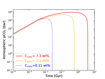
Figure 7: Time evolution of atmospheric pressure with variations in mantle carbon concentration (C_conc) for models assuming an otherwise Earth-like core. An Earth-like initial carbon concentration of 0.011 wt% (not shown) results in an atmospheric mass loss rate always greater than the outgassing rate, so no atmosphere can build up. Models with greater carbon inventories than found on Earth build up temporary secondary atmospheres that are nonetheless lost within 4 Gyr. Even with orders of magnitude greater initial carbon inventory than Earth, GJ 1252b would have no significant remaining atmosphere due to its prodigious atmospheric loss rate.

To further evaluate the prospects for volatile loss from GJ 1252b  we modify the model of Foley & Smye (2018); Foley (2019) to apply to GJ 1252b and explore varying initial mantle CO₂ inventories that will still allow for a completely desiccated planet at the estimated planetary age of $\sim$3.9 Gyr. Mantle gravity and core-radius-fraction model inputs were calculated using the mass-radius-composition solver, ExoPlex (Unterborn & Panero, 2019). As the planet lacks any significant volatile atmosphere, we assumed the planet was made entirely of a FeO-free silicate mantle and pure-liquid-Fe core. Using a planet radius of 1.213 $R_{\oplus}$, mass of 1.32 $M_{\oplus}$ and assuming an Earth-like core radius fraction of 0.55%, ExoPlex calculates an average mantle density of 5026 kg m^-3 and gravity 14.4 m s^-2. Due to the high surface temperature of the planet and the low likelihood of liquid water on the surface, we assume that the planet is in the stagnant lid regime of tectonics (e.g., as is Venus; Gillmann et al., 2022). Our model then assumes all CO₂ outgassed from the mantle will accumulate in the atmosphere, as there is no known method of weathering or recycling carbon without water (Walker et al., 1981; Kasting & Catling, 2003; Foley & Driscoll, 2016). Our model also assumes an Earth-like heat producing element budget, initial mantle temperature of 2000 K, and reference viscosity $\mu_{\mathrm{ref}}=1.3\times 10^{20}\mathrm{~{}Pa~{}s}$ (Foley & Smye, 2018).

Assuming an atmosphere mass loss rate of $5\times 10^{6}$ kg s^-1, we vary the initial mantle CO₂ inventory of our model between an Earth-like initial inventory of 0.011 wt% (mass percentage), based on an estimate of $10^{22}$ mol of CO₂ in the mantle and surface reservoirs of Earth (Sleep & Zahnle, 2001), to 7.3 wt% (over two orders of magnitude greater CO₂ than on present-day Earth, by mass fraction).

Fig. 7 shows the time evolution of total atmospheric pressure with varying initial mantle CO₂ inventories. For the larger carbon inventories considered, the planet’s initial rapid outgassing is greater than the atmospheric loss rate, allowing the atmospheric pressure to build before gradually being eroded once the mantle’s carbon store is depleted. However, for the Earth-like initial CO₂ ($1.1\times 10^{-2}$ wt%) the atmospheric loss rate is always greater than the outgassing rate and so the planet never builds a significant secondary atmosphere. All models tested result in a planet with a completely eroded atmosphere by 3.9 Gyr. Thus GJ 1252b may have had orders of magnitude greater carbon inventory than Earth yet still have no remaining atmosphere today.

Taken together, our model spectra and escape calculations strongly indicate that GJ 1252b has no significant atmosphere.

5 Discussion and Conclusions

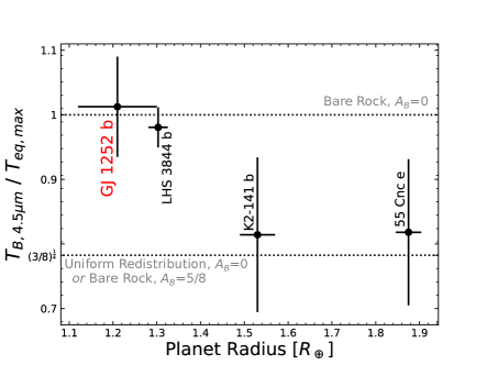
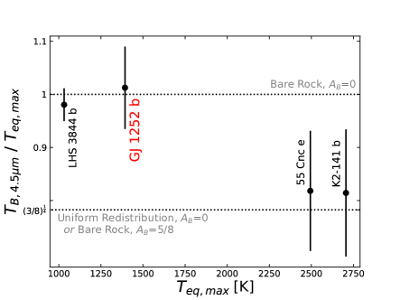
Figure 8: Normalized day-side brightness temperatures, $T_{B,4.5\,\micron}$, of all super-earths with infrared flux measurements plotted vs. planet radius (left) and $T_{\mathrm{eq,max}}$ (right). The two smaller, cooler planets have 4.5 µm brightness temperatures consistent with no atmosphere and zero albedo while the larger, hotter planets are significantly cooler and consistent with uniform redistribution of incident radiation and/or nonzero albedo.

5.1 Comparisons With Similar Exoplanets

GJ 1252b joins the handful of small planets ($<2R_{\oplus}$) with infrared flux detections. The prior examples are 55 Cnc e (whose size and mass imply a sizable volatile mass fraction), LHS 3844b, and K2-141b; some relevant parameters for all these systems (including GJ 1252b) are listed in Table 3. GJ 1252b is smaller than all of these other planets but intermediate in irradiation. We used the system parameters in Table 3, along with BT-Settl model stellar spectra (Allard, 2014) interpolated to these stars’ parameters, to homogeneously calculate the irradiation and 4.5 µm day-side brightness temperatures of all these planets. The model spectra used for all four planets are included as machine-readable files with this paper.

As shown in Fig. 8, a curious dichotomy emerges. The two smallest and coolest planets (GJ 1252b and LHS 3844b) both have day-side brightness temperatures $\left(T_{B,4.5\micron}\right)$ consistent with the maximum possible day-size equilibrium temperature (i.e., $f=\frac{2}{3}$ and $A_{B}=0$ in Eq. 3):

$$T_{\mathrm{eq,max}}=\left(\frac{2}{3}\right)^{1/4}T_{\mathrm{eff}}\sqrt{\frac{R_{*}}{a}}.$$ (4)

On the other hand, the two largest and hottest planets (55 Cnc e and K2-141b) both have notably lower normalized day-side temperatures that are consistent with uniform heat redistribution ($f=\frac{1}{4}$).

This dichotomy may be coincidental: 55 Cnc e’s emission measurements are best interpreted as indicating a massive atmosphere, while the interpretation for K2-141b is a nonzero albedo but negligible atmosphere (Zieba et al., 2022). Some calculations predict that rocky planets with sufficiently intense irradiation could exhibit a high substellar albedo induced by photovolatilization of day-side rocky materials (Kite et al., 2016; Mansfield et al., 2019). One possibility is therefore that there is an irradiation threshold for this albedo enhancement, with GJ 1252b and LHS 3844b lying below it and K2-141b lying above it.

Alternatively, both 55 Cnc e and K2-141b may have atmospheres thick enough that they can transport sufficient heat to measurably cool their day-sides. Evidence of 55 Cnc e’s thick atmosphere is seen in its asymmetric 4.5 µm phase curve (Demory et al., 2016b), but K2-141b’s 4.5 µm phase curve showed no such evidence for a thick atmosphere (Zieba et al., 2022) – this despite K2-141b’s day-side being heated high enough above the silicate solidus that an optically thick, $\sim$0.1 bar mineral atmosphere is predicted. Future modeling and observations will both be needed to determine whether Fig. 8 represents a coherent trend between some combination of irradiation, planet size, heat redistribution, and albedo.

Fortunately, GJ 1252 is bright enough to offer high S/N while faint enough to be observable with all of JWST’s instruments. With an Emission Spectroscopy Metric (ESM; Kempton et al., 2018) greater than K2-141b and within a factor of two of LHS 3844b (see Table 3), GJ 1252b is likely to join the select group of eminently observable and highly irradiated terrestrial exoplanets and to be subjected to many productive future investigations.

Table 3: Planets $<2R_{\oplus}$ and With Measured Infrared Emission

Parameter	GJ 1252b	LHS 3844b	K2-141 b	55 Cnc e
$R_{p}/R_{\oplus}$	1.180	$1.32$	$1.53$	$1.88$
$a/R_{*}$	$5.03$	7.08	2.36	3.51
$T_{\mathrm{eff}}$ / K	$3458$	$3036$	4599	$5172$
$T_{\mathrm{eq,max}}$ / K	1390	1030	2705	2550
$\delta_{4.5\,\micron}$ / ppm	0pt${}^{+25}_{-32}$	$380\pm 40$	$143\pm 39$	$83\pm 23$
$T_{B,4.5\,\micron}$ / K	1410${}^{+91}_{-125}$	$1011^{+32}_{-33}$	$2200^{+310}_{-330}$	$2040^{+270}_{-290}$
ESM${}_{7.5\,\micron}$	16.7	30.0	15.4	70.1

5.2 Conclusions

We have presented our measurement of 4.5 µm thermal emission from the highly irradiated terrestrial planet GJ 1252b. With a radius of just 1.180 $R_{\oplus}$, our target is the smallest planet for which such a measurement has been reported. After presenting our Spitzer data analysis, along with an updated transit analysis using new TESS data in Sec. 2, Sec. 3 compared this measurement to a large suite of atmospheric models and simulated spectra. Our modeling demonstrated that for a broad range of possible atmospheric compositions surface pressures $P_{\mathrm{surf}}\lesssim 10$ bar are required to be consistent with the measured eclipse at 2$\sigma$ confidence. Furthermore, Sec. 4 then showed that the energy-limited atmospheric mass loss from GJ 1252b could quickly erode atmospheres with $P_{\mathrm{surf}}>100$ bar on timescales far shorter than the system lifetime.

We therefore conclude that GJ 1252b possesses no significant atmosphere. In this case, it presumably retains only a tenuous mineral exosphere; such an atmosphere would be expected to have $P_{\mathrm{surf}}\lesssim 10^{-6}$ bar and to be dominated by species such as Na, molecular O₂ and atomic O, and K (Miguel et al., 2011; Ito et al., 2015). Such an atmosphere is likely thin enough that atmospheric circulation would contribute negligibly to global heat and mass transfer (e.g., Nguyen et al., 2020), although detailed simulations will be needed to confirm this. Since GJ 1252b’s atmosphere would be quite optically thin, observations of GJ 1252b therefore offer the opportunity to directly probe surface minerology via emission spectroscopy during eclipse and throughout the planet’s orbit.

Infrared emission has been measured from only three exoplanets with sizes placing them firmly in the terrestrial planet regime. A larger sample is urgently needed to better identify the surface and atmospheric properties of this class of planets; fortunately, this number is already set to increase somewhat in the dawning JWST era (see discussion by Zieba et al., 2022). A further pressing need is to obtain more precise mass measurements for these planets: no mass has been reported for LHS 3844b and GJ 1252b has only a roughly 3$\sigma$ mass. The combination of more precise masses and bulk densities, more precise eclipse spectra, and stellar abundance measurements will ultimately enable more accurate models to link these planets’ surface minerologies and atmospheres to their observed thermal emission.

Fig. 9 shows the joint posteriors on eclipse depth and time of eclipse for our primary, joint analysis. Figs. 10 and 11 show the raw Spitzer photometry for each individual eclipse visit, the photometry after removal of systematics, and the residuals to the fits. Fig. 12 shows how the residuals to these individual fits bin down with time.

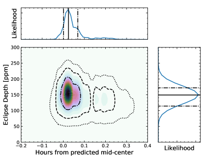
Figure 9: Joint posterior distributions of eclipse depth and time of eclipse center from the analysis plotted in Fig. 2. The eclipse depth exhibits no covariance with the eclipse timing, despite the latter’s long tail toward high values,

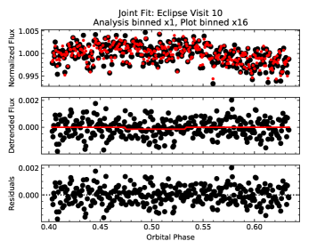
Figure 10: Spitzer 4.5 µm light curves for our joint analysis of all eclipse visits. In each triptych the top panel shows the raw Spitzer photometry (black circles) vs. the PLD model (red points); the middle panel shows the systematics-corrected photometry (black circles) vs. the best-fit eclipse model (red line); the bottom panel shows the residuals. Although we performed our analysis without binning the data, the data are binned here by a factor of 16 for plotting purposes. Fig. 2 shows the stacked average of all ten eclipses.

Figure 11: Same as Fig. 10, but for the final four Spitzer eclipse visits.

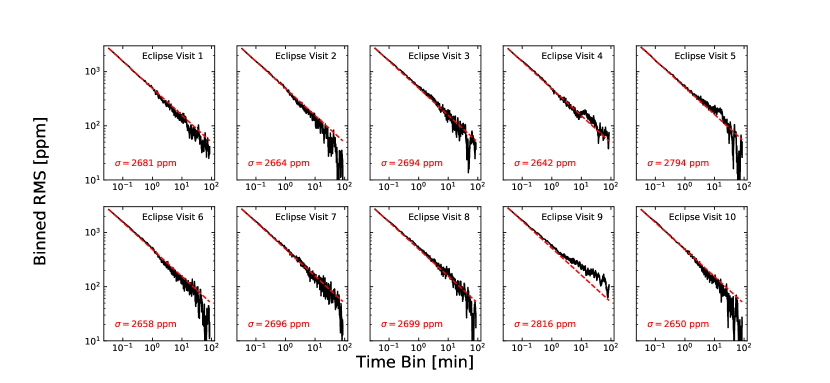
Figure 12: The dispersion of the binned residuals (solid black line) to the 4.5 µm light curves show limited evidence for correlated noise. The dashed line shows the expectation for wholly uncorrelated errors, which scale as $N^{-1/2}$.

References

- Allard (2014) Allard, F. 2014, in IAU Symposium, Vol. 299, IAU Symposium, ed. M. Booth, B. C. Matthews, & J. R. Graham, 271–272
- Angelo & Hu (2017) Angelo, I., & Hu, R. 2017, AJ, 154, 232
- Batalha et al. (2011) Batalha, N. M., Borucki, W. J., Bryson, S. T., et al. 2011, ApJ, 729, 27
- Bourrier et al. (2018) Bourrier, V., Dumusque, X., Dorn, C., et al. 2018, A&A, 619, A1
- Burrows et al. (2008) Burrows, A., Budaj, J., & Hubeny, I. 2008, ApJ, 678, 1436
- Burt et al. (2020) Burt, J. A., Nielsen, L. D., Quinn, S. N., et al. 2020, AJ, 160, 153
- Claret (2017) Claret, A. 2017, A&A, 600, A30
- Cox (2000) Cox, A. N. 2000, Allen’s astrophysical quantities ((New York: AIP Press))
- Crossfield et al. (2018) Crossfield, I., Werner, M., Dragomir, D., et al. 2018, Spitzer Transits of New TESS Planets, Spitzer Proposal
- Crossfield et al. (2015) Crossfield, I. J. M., Petigura, E., Schlieder, J. E., et al. 2015, ApJ, 804, 10
- Crossfield et al. (2016) Crossfield, I. J. M., Ciardi, D. R., Petigura, E. A., et al. 2016, ApJS, 226, 7
- Dang et al. (2020) Dang, L., Calchi Novati, S., Carey, S., & Cowan, N. B. 2020, MNRAS, 497, 5309
- Deming et al. (2015) Deming, D., Knutson, H., Kammer, J., et al. 2015, ApJ, 805, 132
- Demory et al. (2016a) Demory, B.-O., Gillon, M., Madhusudhan, N., & Queloz, D. 2016a, MNRAS, 455, 2018
- Demory et al. (2016b) Demory, B.-O., Gillon, M., de Wit, J., et al. 2016b, Nature, 532, 207
- Engle & Guinan (2018) Engle, S. G., & Guinan, E. F. 2018, Research Notes of the American Astronomical Society, 2, 34
- Esposito (1984) Esposito, L. W. 1984, Science, 223, 1072
- Essack et al. (2020) Essack, Z., Seager, S., & Pajusalu, M. 2020, ApJ, 898, 160
- Fazio et al. (2004) Fazio, G. G., Hora, J. L., Allen, L. E., et al. 2004, ApJS, 154, 10
- Foley (2019) Foley, B. J. 2019, ApJ, 875, 72
- Foley & Driscoll (2016) Foley, B. J., & Driscoll, P. E. 2016, Geochemistry, Geophysics, Geosystems, 17, 1885
- Foley & Smye (2018) Foley, B. J., & Smye, A. J. 2018, Astrobiology, 18, 873
- Foreman-Mackey et al. (2021) Foreman-Mackey, D., Luger, R., Agol, E., et al. 2021, arXiv e-prints, arXiv:2105.01994
- France et al. (2016) France, K., Parke Loyd, R. O., Youngblood, A., et al. 2016, ApJ, 820, 89
- Fulton & Petigura (2018) Fulton, B. J., & Petigura, E. A. 2018, AJ, 156, 264
- Gaillard & Scaillet (2014) Gaillard, F., & Scaillet, B. 2014, Earth and Planetary Science Letters, 403, 307
- Gillmann et al. (2022) Gillmann, C., Way, M. J., Avice, G., et al. 2022, arXiv e-prints, arXiv:2204.08540
- Goldblatt (2015) Goldblatt, C. 2015, Astrobiology, 15, 362
- Gordon et al. (2017) Gordon, I., Rothman, L., Hill, C., et al. 2017, Journal of Quantitative Spectroscopy and Radiative Transfer, 203, 3 , hITRAN2016 Special Issue
- Gordon et al. (2022) Gordon, I., Rothman, L., Hargreaves, R., et al. 2022, Journal of Quantitative Spectroscopy and Radiative Transfer, 277, 107949
- Grimm & Heng (2015) Grimm, S. L., & Heng, K. 2015, ApJ, 808, 182
- Grimm et al. (2021) Grimm, S. L., Malik, M., Kitzmann, D., et al. 2021, ApJS, 253, 30
- Hammond & Pierrehumbert (2017) Hammond, M., & Pierrehumbert, R. T. 2017, ApJ, 849, 152
- Hansen (2008) Hansen, B. M. S. 2008, ApJS, 179, 484
- Henning et al. (2009) Henning, W. G., O’Connell, R. J., & Sasselov, D. D. 2009, ApJ, 707, 1000
- Hong & Fegley (1997) Hong, Y., & Fegley, B. 1997, Icarus, 130, 495
- Howard (2022) Howard, W. S. 2022, MNRAS, 512, L60
- Hu et al. (2012) Hu, R., Ehlmann, B. L., & Seager, S. 2012, ApJ, 752, 7
- Ito et al. (2015) Ito, Y., Ikoma, M., Kawahara, H., et al. 2015, ApJ, 801, 144
- Kane et al. (2014) Kane, S. R., Kopparapu, R. K., & Domagal-Goldman, S. D. 2014, ApJ, 794, L5
- Kane et al. (2020) Kane, S. R., Roettenbacher, R. M., Unterborn, C. T., Foley, B. J., & Hill, M. L. 2020, PSJ, 1, 36
- Kane et al. (2019) Kane, S. R., Arney, G., Crisp, D., et al. 2019, Journal of Geophysical Research (Planets), 124, 2015
- Kasting & Catling (2003) Kasting, J. F., & Catling, D. 2003, ARA&A, 41, 429
- Kempton et al. (2018) Kempton, E. M. R., Bean, J. L., Louie, D. R., et al. 2018, PASP, 130, 114401
- Kite et al. (2016) Kite, E. S., Fegley, Bruce, J., Schaefer, L., & Gaidos, E. 2016, ApJ, 828, 80
- Koll (2022) Koll, D. D. B. 2022, ApJ, 924, 134
- Korenaga (2010) Korenaga, J. 2010, ApJ, 725, L43
- Kreidberg et al. (2019) Kreidberg, L., Koll, D. D. B., Morley, C., et al. 2019, Nature, 573, 87
- Lammer et al. (2019) Lammer, H., Sproß, L., Grenfell, J. L., et al. 2019, Astrobiology, 19, 927
- Li et al. (2015) Li, G., Gordon, I. E., Rothman, L. S., et al. 2015, The Astrophysical Journal Supplement Series, 216, 15
- Lightkurve Collaboration et al. (2018) Lightkurve Collaboration, Cardoso, J. V. d. M., Hedges, C., et al. 2018, Lightkurve: Kepler and TESS time series analysis in Python, Astrophysics Source Code Library, record ascl:1812.013, ascl:1812.013
- Loyd et al. (2016) Loyd, R. O. P., France, K., Youngblood, A., et al. 2016, ApJ, 824, 102
- Luger & Barnes (2015) Luger, R., & Barnes, R. 2015, Astrobiology, 15, 119
- Madhusudhan (2012) Madhusudhan, N. 2012, ApJ, 758, 36
- Malavolta et al. (2018) Malavolta, L., Mayo, A. W., Louden, T., et al. 2018, AJ, 155, 107
- Malik et al. (2019a) Malik, M., Kempton, E. M. R., Koll, D. D. B., et al. 2019a, ApJ, 886, 142
- Malik et al. (2019b) Malik, M., Kitzmann, D., Mendonça, J. M., et al. 2019b, AJ, 157, 170
- Malik et al. (2017) Malik, M., Grosheintz, L., Mendonça, J. M., et al. 2017, AJ, 153, 56
- Mandel & Agol (2002) Mandel, K., & Agol, E. 2002, ApJ, 580, L171
- Mansfield et al. (2019) Mansfield, M., Kite, E. S., Hu, R., et al. 2019, ApJ, 886, 141
- Miguel et al. (2011) Miguel, Y., Kaltenegger, L., Fegley, B., & Schaefer, L. 2011, ApJ, 742, L19
- Millholland & Laughlin (2019) Millholland, S., & Laughlin, G. 2019, Nature Astronomy, 3, 424
- Modirrousta-Galian et al. (2021) Modirrousta-Galian, D., Ito, Y., & Micela, G. 2021, Icarus, 358, 114175
- Nguyen et al. (2020) Nguyen, T. G., Cowan, N. B., Banerjee, A., & Moores, J. E. 2020, MNRAS, 499, 4605
- Polyansky et al. (2018) Polyansky, O. L., Kyuberis, A. A., Zobov, N. F., et al. 2018, MNRAS, 480, 2597
- Richard et al. (2012) Richard, C., Gordon, I. E., Rothman, L. S., et al. 2012, J. Quant. Spec. Radiat. Transf., 113, 1276
- Rothman et al. (2010) Rothman, L., Gordon, I., Barber, R., et al. 2010, JQSRT, 111, 2139
- Salz et al. (2015) Salz, M., Schneider, P. C., Czesla, S., & Schmitt, J. H. M. M. 2015, A&A, 576, A42
- Salz et al. (2016) —. 2016, A&A, 585, L2
- Savitzky & Golay (1964) Savitzky, A., & Golay, M. J. E. 1964, Analytical Chemistry, 36, 1627
- Schaefer et al. (2016) Schaefer, L., Wordsworth, R. D., Berta-Thompson, Z., & Sasselov, D. 2016, ApJ, 829, 63
- Seager (2010) Seager, S. 2010, Exoplanet Atmospheres: Physical Processes
- Sheets & Deming (2014) Sheets, H. A., & Deming, D. 2014, ApJ, 794, 133
- Shporer et al. (2020) Shporer, A., Collins, K. A., Astudillo-Defru, N., et al. 2020, ApJ, 890, L7
- Sleep & Zahnle (2001) Sleep, N. H., & Zahnle, K. 2001, J. Geophys. Res., 106, 1373
- Sneep & Ubachs (2005) Sneep, M., & Ubachs, W. 2005, J. Quant. Spec. Radiat. Transf., 92, 293
- Stassun et al. (2018) Stassun, K. G., Oelkers, R. J., Pepper, J., et al. 2018, AJ, 156, 102
- Tamburo et al. (2018) Tamburo, P., Mandell, A., Deming, D., & Garhart, E. 2018, AJ, 155, 221
- Thalman et al. (2014) Thalman, R., J. Zarzana, K., Tolbert, M., & Volkamer, R. 2014, Journal of Quantitative Spectroscopy and Radiative Transfer, 147, 171–177
- Underwood et al. (2016) Underwood, D. S., Tennyson, J., Yurchenko, S. N., et al. 2016, Monthly Notices of the Royal Astronomical Society, 459, 3890
- Unterborn & Panero (2019) Unterborn, C. T., & Panero, W. R. 2019, Journal of Geophysical Research (Planets), 124, 1704
- Vanderspek et al. (2019) Vanderspek, R., Huang, C. X., Vanderburg, A., et al. 2019, ApJ, 871, L24
- Wagner & Kretzschmar (2008) Wagner, W., & Kretzschmar, H.-J. 2008, International Steam Tables - Properties of Water and Steam Based on the Industrial Formulation IAPWS-IF97 (Springer, Berlin, Heidelberg), doi:https://doi.org/10.1007/978-3-540-74234-0
- Walker et al. (1981) Walker, J. C. G., Hays, P. B., & Kasting, J. F. 1981, J. Geophys. Res., 86, 9776
- Winn (2010) Winn, J. N. 2010, ArXiv e-prints, arXiv:1001.2010
- Wordsworth & Kreidberg (2021) Wordsworth, R., & Kreidberg, L. 2021, arXiv e-prints, arXiv:2112.04663
- Wordsworth & Pierrehumbert (2014) Wordsworth, R., & Pierrehumbert, R. 2014, ApJ, 785, L20
- Youngblood et al. (2016) Youngblood, A., France, K., Loyd, R. O. P., et al. 2016, ApJ, 824, 101
- Yurchenko et al. (2017) Yurchenko, S. N., Amundsen, D. S., Tennyson, J., & Waldmann, I. P. 2017, A&A, 605, A95
- Zahnle & Catling (2017) Zahnle, K. J., & Catling, D. C. 2017, ApJ, 843, 122
- Zhang et al. (2012) Zhang, X., Liang, M. C., Mills, F. P., Belyaev, D. A., & Yung, Y. L. 2012, Icarus, 217, 714
- Zieba et al. (2022) Zieba, S., Zilinskas, M., Kreidberg, L., et al. 2022, arXiv e-prints, arXiv:2203.00370