Haifa, 32000, Israel
bbinstitutetext: School of Science, Huzhou University
Huzhou 313000, Zhejiang, China ccinstitutetext: Center for Gravitational Physics and Quantum Information
Yukawa Institute for Theoretical Physics, Kyoto University
Kitashirakawa-Oiwakecho, Sakyo-ku, Kyoto 606-8502, Japan
The holography of duality in Super-Yang-Mills theory
Abstract
The space of supersymmetric Yang-Mills theories exhibits an intricate structure of global one-form symmetries and duality orbits. In this paper we study this structure from the point of view of the holographic dual Type IIB string theory. Generalizing work by Witten, we map the different theories based on the gauge algebras , , and to a choice of boundary conditions on bulk gauge fields. We show how the one-form symmetries and their anomalies, as well as the duality properties of the gauge theories, arise in the holographic picture. Along the way we prove that the number of disjoint duality orbits for the theories is given by the number of square divisors of .
1 Introduction
One of the most interesting properties of SYM theory is duality, namely the property that one SYM theory with a given value of the complexified coupling parameter is physically equivalent to another, generically different, SYM theory with a different value of , given by an action by an element of a discrete duality group on the original value. For simply laced gauge groups the duality group is , which is generated by the GNO-duality transformation, and the perturbative transformation that shifts the Yang-Mills theta angle by . For non-simply laced groups the duality group is slightly different. The duality acts on the gauge algebra in a simple way: acts trivially, and maps the algebra to the GNO-dual algebra . On the other hand the action of the duality on the gauge theories turns out to be rather intricate Aharony:2013hda . For example the theory with is related by to the theory with . More generally gauge theories based on the same algebra can differ in the global structure of the gauge group, as well as in values of discrete theta-like parameters. The different theories have the same spectrum of local operators, but a different spectrum of extended line operators Aharony:2013hda , and correspondingly a different global one-form symmetry Gaiotto:2014kfa . The different gauge theories based on and are related by the duality, but generically form several disjoint duality orbits Aharony:2013hda . In particular for with square-free there is only one duality orbit, but otherwise there are more.
The correspondence, the most famous example of which relates SYM theory to Type IIB string theory in , provides an alternative and complementary point of view on these topics. Soon after Maldacena’s discovery of Maldacena:1997re , Witten showed that different theories based on correspond to different choices of boundary conditions for the NSNS and RR 2-form gauge fields and in Witten:1998wy . In particular any theory related by an duality transformation to the theory with corresponds to a boundary condition on that is related by the same element of the symmetry of Type IIB string theory to the boundary condition on corresponding to the theory.
In this paper we will extend Witten’s results to include all the SYM theories based on the , , , and algebras. We will match all the different gauge theories of Aharony:2013hda to a corresponding set of boundary conditions on the appropriate gauge fields in the dual background. Using the dual Type IIB string theory description we will reproduce the spectrum of line operators, the one-form symmetries and their anomalies, as well as the structure of the duality orbits. Along the way we will also prove that the number of duality orbits for the theories based on is given by the number of square divisors of .
The rest of the paper is organized according to the gauge algebras. In section 2 we discuss the theories. We begin by reviewing the results of Aharony:2013hda ; Gaiotto:2014kfa on the different theories and their one-form global symmetries, and how they are related by duality. We also review two mixed anomalies in this class of theories following Hsin:2020nts and Cordova:2019uob . We then discuss the holographic description of the different theories in terms of the boundary conditions imposed on the NSNS and RR 2-form fields in the bulk, and how the spectrum of line operators and one-form symmetries of the gauge theories are realized in terms of branes in the bulk. We also explain how the 5d anomaly actions corresponding to the mixed anomalies arise as Chern-Simons terms in the supergravity action. Finally, we provide a brane realization, and the corresponding fully backreacted supergravity solution, of an interface in the gauge theory, separating regions with theta parameters differing by a multiple of . In section 3 we discuss the theories, starting again with a review of the results of Aharony:2013hda on the spectrum of line operators and the action of duality. We then move to the holographic description, find the dual boundary conditions, and discuss the brane realization of the line operators and one-form symmetries. In particular we highlight the distinction between and , and the distinction between and . Section 4 contains the analogous discussion of the and theories. Section 5 contains our conclusions and future directions.
2 The theories
2.1 One form symmetry and duality
YM theories with gauge algebra are characterized in general by the global structure of the gauge group, , where is a divisor of , and by the value of a discrete theta-like parameter taking values in Aharony:2013hda . The local properties of all the theories are the same, but the spectrum of line operators depends on and :
| (1) |
where and . A priori the charges take values in the center of , but they are constrained by mutual locality via the Dirac pairing condition
| (2) |
It was argued in Aharony:2013hda that for a consistent quantum field theory the set of charges must be maximal and complete. The different maximal sets can be represented as .
The different theories are related by duality in a non-trivial way Aharony:2013hda . The generator of takes , and therefore
| (3) |
The generator takes , which implies that
| (4) |
where is a member of a Bezout pair of integers associated to the pair .111This is determined by finding the minimal charges in of the form and . For these are given by , and therefore . Then for we have and , which implies that are a Bezout pair associated to . For example maps the theory to the theory, and then acting with leads to all the other theories. However in general not all theories are related by to the theory. This is only the case if is square-free, i.e. if all of its prime factors appear only once Aharony:2013hda . More generally the theories form different orbits under . As we will show below, the number of different orbits is equal to the number of different square divisors of , and is therefore given by
| (5) |
where is the integer part of , and is the exponent of the prime in the prime factorization of ,
| (6) |
For a square-free integer all are either 0 or 1, and therefore .
The structure of the different theories can also be described in terms of higher form symmetry Gaiotto:2014kfa . The theory has a global one-form symmetry, corresponding to the center of , acting on “electric” Wilson lines in arbitrary representations of . The charge of a Wilson line is given by the -ality of the representation, i.e. the number of boxes in the corresponding Young diagram. The theory is obtained by gauging a subgroup of . This removes electric lines with charges that are not a multiple of , leaving an electric one-form symmetry acting on the remaining electric lines. The new theory also admits additional line operators carrying magnetic charges that are multiples of . If these lines carry no electric charge then they are acted on by a magnetic one-form symmetry , and the total one-form symmetry is . If and are mutually prime this is equivalent to . More generally the spectrum of line operators is given by (1), and the one-form symmetry of the theory is given by
| (7) |
The first factor acts on the electric lines , the second factor acts on the dyonic lines , and the quotient accounts for the relation mod . This can be more simply expressed as
| (8) |
by bringing the matrix of fundamental line charges to Smith normal form:
| (13) |
where are matrices.222The explicit transformation is presented in Appendix A. For this reduces to .
The transformation in (13) shows that any theory of the form may be mapped by duality to the theory , with .333Indeed the quantity is invariant under . Under the transformation , and under the transformation , where we have used the fact that implies that that the integers and are a co-prime pair. The different orbits are therefore classified by the possible values of . For example for there are two separate orbits of theories corresponding to and . The former contains the six theories , , and , and the latter contains just the theory Aharony:2013hda . The number of orbits for is given by the number of distinct values that the integer can have. Since we can take the seed theory for each orbit to be , this translates to the number of different divisors of satisfying , or equivalently to the number of square divisors of .
2.2 Anomalies
There is a mixed anomaly between the and factors in the one-form symmetry (8) determined by the extension
| (14) |
The degree of the anomaly is equal to the degree of the extension, which is . For the special case of this is a mixed anomaly between the electric one-form symmetry and the magnetic one-form symmetry Gaiotto:2014kfa . The 5d anomaly action in this case is given by Hsin:2020nts
| (15) |
where and are background fields of the electric and magnetic symmetries, respectively, namely
| (16) |
The order of the anomaly in this case is . We can see this explicitly using the fact that we can write for some pair of integers , and multiplying the anomaly action by this quantity. Integrating the second term by parts gives
| (17) |
and since and , this is a multiple of .
More generally we have and . If the order of the anomaly is reduced to . This can be seen by performing the following change of basis
| (18) | |||||
| (19) |
where is an integer satisfying
| (20) |
and is a pair of integers satisfying
| (21) |
(See the Appendix A for the proof of their existence). It follows that
| (22) | |||||
| (23) |
We can then express the anomaly action as
| (24) |
where the last two terms can be cancelled by 4d counterterms. This has the same form as (15) with replaced by . Therefore the order of the anomaly is .
There is another kind of mixed anomaly in these theories that involves the electric one-form symmetry and the periodicity of the parameter Cordova:2019uob . For example in the theory the parameter has a periodicity, . Turning on a background field for the electric one-form symmetry leads to a phase in the path integral under ,
| (25) |
A non-trivial corresponds to a fractional instanton, an bundle that cannot be lifted to an bundle. Gauging the one-form symmetry, by summing over all elements , would then violate the periodicity of .444For this also implies that there is a mixed anomaly between the one-form symmetry and time reversal Gaiotto:2017yup . We can express this anomaly in terms of a 5d anomaly action given by
| (26) |
Note that the part of the anomaly, namely the in the numerator, is trivial for spin manifolds, since is an even integer for spin manifolds. The same anomaly action (26) holds more generally for the theory. In this case the periodicity of the parameter increases to , and the analogous phase in the path integral is given by
| (27) |
where now . Note that is still the background field of the electric one-form symmetry, which is the subgroup of (7) or (8).
2.3 Holography
The holographic dual of SYM theory with gauge algebra is Type IIB string theory on Maldacena:1997re . The global structure of the theory depends on the boundary conditions satisfied by the NSNS and RR 2-forms Witten:1998wy . These boundary conditions are constrained by a 5d Chern-Simons term
| (28) |
which is the dominant term near the boundary of . This implies that the boundary values of and are flat, and therefore completely characterized by their holonomies on closed two-surfaces at the boundary,555What one should really have in mind is a topologically non-trivial boundary with homology 2-cycles, such as .
| (29) | |||||
| (30) |
The CS action also implies that and are quantum-mechanically conjugate variables, and in particular that
| (31) |
where is the intersection number of the surfaces and . In other words generates a “translation” symmetry acting on as , and vice versa. The quantum mechanical variables and can therefore be viewed as discrete position-like and momentum-like variables taking values in :
| (32) |
with
| (33) |
The different boundary theories correspond to a choice of a maximal set of commuting observables. The set must be maximal, since every quantum state is a simultaneous eigenstate of a maximal set of commuting observables.666This can be shown as follows. Let be a simultaneous eigenstate of a maximal set of commuting observables , namely . Let be an arbitrary state in the Hilbert space. Then there exists a unitary operator such that . We then have , and therefore the state is a simultaneous eigenstate of the maximal set of commuting observables . We thank Shlomo Razamat for the proof. For example if we choose to fix at the boundary we can only simultaneously fix , which means that is free as an element of . The state in this case is dual to the theory. More generally the set of observables of the form
| (34) |
that we can simultaneously fix at the boundary must satisfy
| (35) |
This is precisely the Dirac pairing condition of (2). In other words the condition of mutual locality of the line operators in the boundary theory corresponds to the condition of mutual commutativity of the observables in the bulk. Furthermore, the requirement that the the spectrum of line operators be maximal follows from the requirement that the set of observables be maximal. The maximal set has at most two independent observables satisfying . By a convenient choice of basis we can set
| (36) |
where and . This pair of observables corresponds to the theory. In particular we can read off the one form symmetry (7) from the observables that are fixed at the boundary. The observable gives the factor, the observable gives the factor, and the relation gives the quotient by .
Once we have identified the boundary conditions dual to the gauge theory, the action of on the gauge theory follows from the action of in Type IIB string theory. The generator takes and therefore
| (37) |
which reproduces (3). The generator takes and therefore
| (38) |
We can recast these in the form of (4) by a change of basis
| (45) |
where are a Bezout pair associated to .
2.4 Holographic anomaly actions
Anomaly actions are a useful way of encoding anomalies in terms of “anomaly inflow” from a fictional space with one more dimension. In holography this space is real, and the anomaly actions are part of the bulk physics. They are given by Chern-Simons terms in the bulk. In our case the relevant CS term is (28). The Type IIB 2-form gauge fields and are the continuum versions of the background fields and . Identifying and , we see that the 5d CS action (28) reproduces the 5d anomaly action of the first mixed anomaly (15).
The second mixed anomaly involves the parameter, which is realized in the bulk in terms of the RR scalar field . There is no bulk CS term in Type IIB supergravity that involves this field directly. However couples indirectly to the NSNS 2-form via the modified RR 3-form field strength,
| (46) |
It is this combination that appears in the kinetic term. This allows us to rewrite the CS term in (28) as
| (47) |
The first term reproduces the part of the anomaly action in (26). The part is missing. On the other hand, since we are considering a supersymmetric theory, and are therefore restricted to spin manifolds, the part of the anomaly is anyway trivial.
2.5 Branes, lines, and surfaces
Line operators in the 4d gauge theory correspond to one-dimensional boundaries of string worldsheets that end on the boundary of . The 4d theory also has two-dimensional surface operators described in the bulk by string worldsheets approaching, and parallel to, the boundary. These surface operators implement the one-form symmetries acting on the line operators. The spectrum of line and surface operators, and correspondingly the one-form symmetry group, depends crucially on the boundary conditions on .
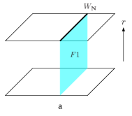
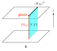
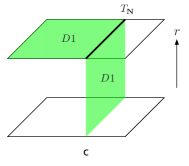
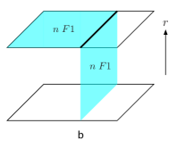
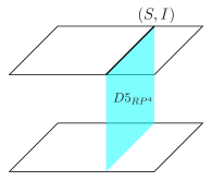
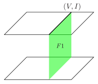
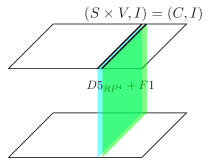
Consider for example the theory. The fixed boundary condition on the NSNS holonomy implies that the worldsheet of a fundamental string (or F-string) at the boundary corresponds to a trivial surface operator. On the other hand the free boundary condition on the RR holonomy implies that the worldsheet of a D-string at the boundary describes a non-trivial surface operator acting on the line operators described by F-strings ending on the boundary, Fig. 1a.777A more precise description of a surface operator is given by an D3-brane with magnetic flux perpendicular to the 2-surface which represents a D-string Gukov:2006jk ; Drukker:2008wr . That the one-form symmetry is is seen in the bulk by the screening of F-strings ending on the boundary by a Euclidean D5-brane wrapping and ending on the boundary, Fig. 1b.888One might be concerned with the possibility that this D5-brane might instead attach to a D5-brane at the boundary. However the free boundary condition on , which allows D-strings to approach the boundary, forbids wrapped D5-branes from doing so. This is because Hodge duality exchanges free and fixed boundary conditions. Defining as the 5d gauge field that couples to the wrapped D5-brane, we have (48) where denotes the derivative normal to the boundary, and the derivative tangent to the boundary. This is a Euclidean version of Witten’s Baryon vertex Witten:1998xy . In some sense it identifies the wrapped Euclidean D5-brane as the gluon operator of the 4d gauge theory. D-strings ending on the boundary do not give rise to genuine line operators, since they can attach to a D-string surface at the boundary, Fig. 1c. For the S-dual theory the situation is very similar, with the roles of the F-string and D-string exchanged. Indeed we get basically the same thing for any transform of the theory: the non-trivial line operators are described by worldsheets of -strings ending on the boundary, and such strings are screened by a wrapped Euclidean 5-brane ending on the boundary.
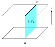
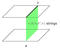
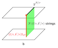
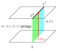
More generally, the first boundary condition in (36) fixing implies that a multiple of F-strings at the boundary corresponds to a trivial surface operator. We therefore have genuine electric lines described by multiples of F-strings ending on the boundary, Fig. 2a. A smaller number of F-strings ending on the boundary can attach to F-strings at the boundary, Fig. 2b. A multiple of F-strings ending on the boundary can be screened by a D5-brane wrapping , Fig. 2c. This explains the factor in (7). The second boundary condition fixing imposes an analogous constraint on strings with . Namely a multiple of -strings at the boundary corresponds to a trivial surface operator, and therefore multiples of such strings ending on the boundary describe genuine dyonic line operators, Fig. 3a. A smaller number of -strings ending on the boundary can attach to strings at the boundary. An multiple of of these strings can be screened by an 5-brane wrapping , Fig. 3b. This explains the factor in (7). Finally, the divisor in (7) corresponds to the identification of -strings with F-strings via an NS5-brane on (Fig. 3c).
Altogether this reproduces the spectrum of line operators in (1), and the one form symmetry in (7), or equivalently (8).

2.6 The interface as a two-face
In pure YM theory, the mixed anomaly at implies that CP is spontaneously broken in the IR, and therefore that there exists a domain wall separating the distinct vacuua with and Gaiotto:2017tne .999Spontaneous CP breaking is actually one of three logical possibilities for the IR theory. The other two are a non-trivial gapless theory or a gapped topological theory. However it is known that CP is spontaneously broken for , and so it is plausible that this is true for finite and large . The anomaly implies that the 3d domain wall theory is an CS theory. The theory, on the other hand, is a conformal field theory, so CP cannot be spontaneously broken, and there is no domain wall. However one can still have a nontrivial interface separating two regions with values of differing by a multiple of , say and . In the pure YM theory the 3d interface theory depends on the magnitude of the derivative of relative to the dynamical scale of the theory Gaiotto:2017tne . For the interface corresponds essentially to domain walls, and the interface theory is . For the interface theory is . There must therefore be a transition between these two theories at some intermediate scale. In contrast, the theory does not have a dynamical scale, and the interface theory is just . Using level-rank duality we can equivalently describe the interface theory as .
The holographic dual of an interface should involve a D7-brane, which sources the Type IIB axion dual to the parameter of the SYM theory. In the original brane configuration in flat space we have:
| 0 | 1 | 2 | 3 | 4 | 5 | 6 | 7 | 8 | 9 | |
| D3 | ||||||||||
| D7 |
This is an brane system and therefore non-supersymmetric. At non-zero separation along , the D3-branes and D7-branes repel each other. Replacing the D3-branes with their near-horizon background, these D7-branes wrap the and are transverse to the and radial coordinates of . The D7-branes are pushed towards the horizon.
A related configuration was studied in Fujita:2009kw . There the coordinate was compactified such that , leading to a background, known as the soliton, in which the circle shrinks at a non-zero radial position . The space is then topologically a disk with the D7-branes located at its center. Taking D7-branes, and ignoring their backreaction on the metric and dilaton, the axion field takes the form
| (49) |
From the point of view of the boundary theory, namely the low-energy 3d worldvolume theory of the compactified D3-branes, this gives a level CS term. On the other hand, from the point of the D7-branes, the 5-form flux on gives a level CS term. Thus this construction gives a holographic realization of level-rank duality.
In our case is not compact, and the dependence of the axion on and is more complicated. But in principle this should provide a realization of an interface that interpolates between and . Remarkably, there exists a fully backreacted solution with precisely this property. This is the axionic Janus (the Roman two-faced god) solution, which we now describe.
The Janus geometry is given by a specific preserving deformation of most easily expressed using the slicing of Bak:2003jk ; DHoker:2006vfr ,
| (50) | |||||
| (51) |
For , the coordinate is related to the usual coordinates as
| (52) |
and it ranges from , corresponding to one half of the boundary with , to , corresponding to the other half of the boundary with . The warp factor for is given by , and the axio-dilaton is a constant. More generally, the reduced equation for the axio-dilaton is given by
| (53) |
Integrating the real part of (53) gives
| (54) |
which can then be used to integrate the equations for the warp factor to give
| (55) |
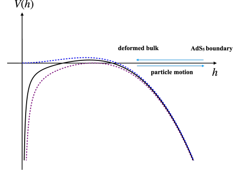
This equation can be viewed as the integrated equation of motion of a zero energy particle in a potential with (see Fig. 4). The particle comes in from infinity, corresponding to one half of the boundary at , and bounces back (at the greatest root of ) to infinity, corresponding to the other half at . The case corresponds to the undeformed solution, for which . More generally . There is a critical value of , given by , above which the particle does not bounce back and reaches the singularity at .
Integrating the imaginary part of (53) gives101010This only holds if is not a constant. If is a constant, the imaginary part of (53) is trivially satisfied, and the solution reduces to the purely dilatonic Janus solution of Bak:2003jk .
| (56) |
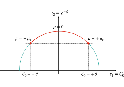
In other words the axio-dilaton resides on a semicircle of radius in the upper half complex plain. The general solution interpolates between a particular value of on this circle on one half of the boundary at and another value on the other half at . Of particular interest to us are trajectories such that the dilaton is the same on both halves of the boundary. For example, if we set , the solution will interpolate between and , Fig. 5. Note that the dilaton remains small everywhere as long as .
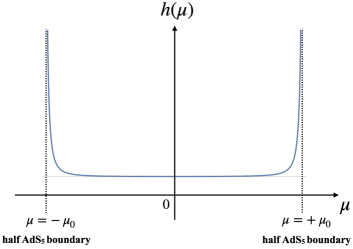
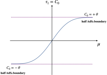
The analytic solution is known and can be expressed in terms of elliptic functions DHoker:2006vfr . In Fig. 6 we present numerical plots of the warp factor and the axion . Note that the axion is a smooth function of , but is a step function as a function of on the boundary. The coordinate relation in (52) can be rewritten as
| (57) |
At the boundary this becomes
| (58) |
Since the Janus geometry is asymptotically , the coordinate relation is essentially the same for , modulo a rescaling of , and we have
| (59) |
Charge quantization requires , where is the number of D7-branes sourcing the Janus deformation.
3 The theories
3.1 One form symmetries and dualities
The different theories are obtained by gauging subgroups of the one-form symmetry of the covering group . The group has four classes of representations: the adjoint, or trivial, class , the vector class , and the two spinor classes and .
For odd the center of is , with the different classes of representations transforming under the generator as
| (60) |
In particular for odd we have the relations , , , and . The possible gauge groups are , , and . The line operator charges take values in , with the generator corresponding to . The Dirac pairing condition is given by
| (61) |
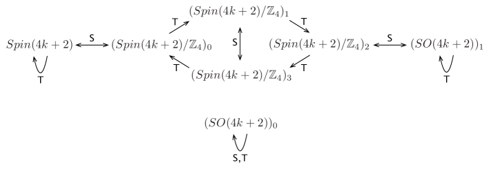
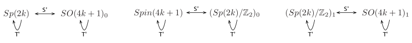
There are seven different maximal charge lattices satisfying this condition. The corresponding theories and their one-form symmetries are shown in Table 1.111111In Aharony:2013hda the additional parameter for was denoted as . Note that this generalizes from the previous section. The action of is shown in Fig. 7. There are two orbits of theories for any , one containing the six theories with , and one with just the theory which has .
| theory | ||
|---|---|---|
For even the center of is , with the different classes transforming as
| (62) |
under the generator of , and as
| (63) |
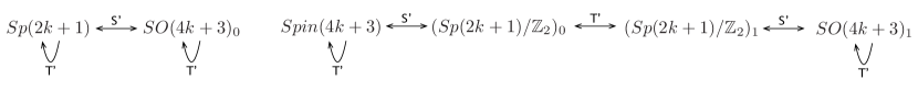
under the generator of . In this case the classes are related as , , , and . The possible gauge groups are , (where is the diagonal subgroup of ), , , and . The line operator charges now take values in , with the generator of corresponding to the spinor class , and the generator of corresponding to the spinor class . The mutual locality condition is now given by Aharony:2013hda
| (64) | |||||
| (65) |
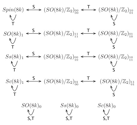
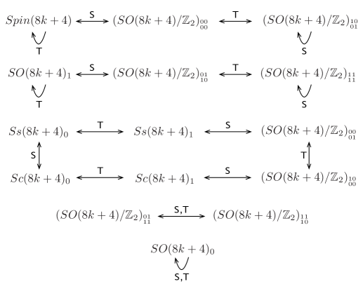
In either case there are fifteen maximal charge lattices, all two-dimensional, as summarized in Table 2.121212For a proof see Appendix B. The action of in the two cases is shown in Figs. 8 and 9.
| theory | ||
|---|---|---|
3.2 Holography
The holographic dual of the theories is , corresponding to the near horizon background of D3-branes on an orientifold 3-plane Witten:1998xy . The orientifold action relates antipodal points on the , and at the same time acts as on both the NSNS and RR 2-form potentials , . The corresponding strings are therefore charged. There are two additional 2-form potentials coming from the reduction of the 6-forms, dual to the NSNS and RR 2-forms in ten dimensions, on the 4-cycle :
| (66) |
These survive the orientifold projection since the volume form of the is odd. The objects that are charged under these fields are 5-branes wrapping , which Witten called “fat strings” in Witten:1998xy . A crucial observation made by Witten in Witten:1998xy is that a pair of identical wrapped 5-branes annihilate into mod strings.131313Witten demonstrated this by constructing a five-dimensional manifold with two boundaries, such that a 5-brane on describes the annihilation process of two 5-branes on . The manifold is in fact isomorphic to the whole compact space , and therefore the 5-brane on has a tadpole due the RR 5-form flux that must be cancelled by attaching to it mod 2 strings. In other words if is even two 5-branes of the same type annihilate into nothing, but if is odd they leave behind a string of an appropriate type. For a pair of D5-branes this is a fundamental string, and for a pair of NS5-branes it is a D-string. The wrapped 5-branes, or “fat strings” correspond to line operators in spinor representations, and the strings correspond to line operators in the vector representation. We will discuss these identifications more below.
The dominant part of the low energy action near the boundary of now has three CS couplings:
| (67) |
The first CS term comes from the ten-dimensional CS term, and the two other CS terms originate from the ten-dimensional kinetic terms for and . As before, this action implies that all the potentials are flat, and characterized entirely by their holonomies . Note that although and are odd under the orientifold action, there is a remnant in the holonomies .
In the quantum theory we can choose as our position operators and . The corresponding conjugate momenta are given by
| (68) |
This implies the non-trivial commutation relations
| (69) |
and
| (70) |
All other commutators vanish mod . However due to the 5-brane annihilation process described above, we have the following constraints relating the variables,
| (71) |
If is odd, namely for , the commutator in (70) implies that and take values in . The constraints (71) imply that and , namely that and take values in . This is consistent with the commutators in (69). The holonomy variables correspond to electric and magnetic spinors, respectively, and to electric and magnetic vectors, respectively. A maximal set of commuting observables of the form then corresponds to a maximal lattice satisfying the condition
| (72) |
So again we see that the condition of mutual commutativity of the boundary conditions corresponds to the condition of mutual locality of the line operators. The resulting assignment of boundary conditions to the theories is shown in Table 3. The action of on the 6-form gauge fields in Type IIB string theory gives
| (73) |
This reproduces the orbits of Fig. 7.
| theory | BC’s |
|---|---|
| , | |
If is even, namely for , the four holonomy variables are independent, and all valued in . The difference between the case and the case is the commutator (70), which is trivial in the former case and non-trivial in the latter case. Now we consider a set of observables of the form . Mutual commutativity requires that for any pair of observables we have
| (74) |
This reproduces the mutual locality conditions for the line operators in (64) once we identify , , , and . The assignment of boundary conditions to the theories is shown in Table 4. The duality orbits of Figs. 8,9 are reproduced by the action of on and .
| theory | boundary conditions |
|---|---|
3.3 Branes and line operators
As before, the line operators in the 4d gauge theory correspond to the boundaries of string worldsheets ending on the boundary of . Now we have both the 10d strings, namely the fundamental strings, the D-strings, and more generally strings, as well as the various “fat strings” corresponding to 5-branes wrapping . The boundaries of the fat strings correspond to line operators in one of the spinor representations of , which we will take to be ,141414This follows from the fermionic zero modes on the 5-3 strings Witten:1998xy . and the boundaries of the ten-dimensional strings correspond to line operators in the vector representation . More specifically, the fundamental string corresponds to an electric vector, the D-string to a magnetic vector, the wrapped D5-brane to an electric spinor , and the wrapped NS5-brane to a magnetic spinor . A line operator in the other spinor representation is described by a bound state of a wrapped 5-brane and the appropriate string. The full spectrum of line operators depends on the boundary conditions on the fields , since these boundary conditions determine which strings are allowed to end on the boundary of . Let us consider just a few examples.
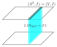
: The dual boundary condition fixes , and therefore also . This means that only wrapped D5-branes and fundamental strings can end on the boundary of , and two wrapped D5-branes are equivalent to one fundamental string. One wrapped D5-brane corresponds to an electric line in the spinor representation , two wrapped D5-branes (or one string) to an electric line in the vector representation , three wrapped D5-branes to an electric line in the spinor representation , and four correspond to a trivial line operator (see Fig. 10). This is precisely the spectrum shown at the top of table 1.
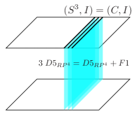
: For even the dual boundary conditions fix and separately. So as in our first example, both D5-branes and fundamental strings can end on the boundary, but here there is no relation between them. In this case one wrapped D5-brane corresponds to electric -line and two are trivial, and one fundamental string corresponds to an electric -line and two are trivial. We can also consider a D5-F1 combination, which corresponds to an electric -line (see Fig. 11). This is precisely the spectrum shown at the top of table 2.

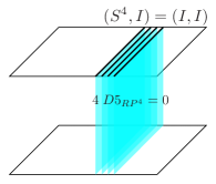
: The dual boundary conditions fix and . For odd these are equivalent to and . This means that only the fundamental string (or equivalently pairs of D5-branes for odd ) and the D-string (or equivalently pairs of NS5-branes for odd ) can end on the boundary. The spectrum of line operators therefore consists of electric and magnetic vectors, in agreement with the second line in both tables 1, 2.
Note that screening by another brane does not play a role here. There is no “baryon vertex” in .
4 The and theories
4.1 One form symmetries and dualities
In either case the center is and so the line operator charges take values in . For the electric charge is carried by the spinor representation and the magnetic charge by the vector representation of the GNO-dual algebra, and vice versa for the algebra . We note also that and . Electric lines in the vector representation of are screened by the Pfaffian operator, which carries one loose gauge index in this case. The Dirac pairing condition is given by
| (75) |
There are three different theories in either case, see Table 5.
| theory | ||
|---|---|---|
The duality group in this case is not exactly , but rather the subgroup generated by Dorey:1996hx ; Girardello:1995gf
| (80) |
This acts in the standard way on the properly normalized complexified coupling,
| (81) |
where
| (82) |
In particular
| (83) |
This subtlety will be important when we discuss the string theory dual. The duality orbits are slightly different for even and odd , and are show in Figs. 12,13.
4.2 Holography
The background admits torsion-valued fluxes of the RR and NSNS 2-forms given by Witten:1998xy . The four possibilities correspond to the four O3-plane variants: and Hanany:2000fq . The trivial flux background with , corresponding to the plane, was discussed in the previous section. This is dual to the theories. The three other backgrounds with , , and , correspond, respectively to the , , and planes, and are dual, respectively, to the , , and theories. The theories are based on the same algebra as the theories, but differ from them in the spectrum of magnetically charged states on the Coulomb branch Hanany:2000fq . In what follows we will concentrate on the and backgrounds, and briefly comment on the background and the dual theories in a separate section.
While the background is invariant under the symmetry of Type IIB string theory, the other backgrounds transform as follows:
| (84) |
These transformations are clearly related to the duality transformations of the gauge theory, however this relation is not as straightforward as in the previous cases. We start by noting that the Type IIB axio-dilaton is related to the complexified coupling of the gauge theory as follows:
| (85) |
The Type IIB supergravity action is given in the Einstein frame by
| (86) |
where
| (89) |
Consider the simple field redefinition
| (90) |
It follows that
| (91) |
Under the action
| (92) |
and therefore
| (93) |
This is precisely what one would get by acting with the generator of , so we find that . On the other hand under the action of
| (94) |
which translates to the action on and
| (95) |
and therefore . This implies in particular that the set of theories based on and the set based on , dual to the and backgrounds, are separately invariant under . As we mentioned above, we will discuss the background and the theories in a separate section.
The 5d CS action is the same as before (67), but there are additional constraints on the fields due to the torsion NSNS or RR flux. Recall that in the background we had the constraints (71) for odd originating from a condition on wrapped 5-branes. These constraints continue to hold in the other backgrounds. The additional constraints arise from additional conditions on wrapped branes Witten:1998xy . The first is a topological restriction on wrapping 5-branes: a D5-brane (NS5-brane) can wrap only if (). More generally there is an obstruction to wrapping an odd number of D5-branes (or NS5-branes) if (or ). We interpret this as a constraint on (or ) allowing only classes that are even multiples of the generator. The second condition is on the D3-brane wrapping . The RR (NSNS) flux gives rise to a tadpole which must be cancelled by attaching a fundamental string (D-string) to the D3-brane. Equivalently, this means that a fundamental string can be screened by a wrapped D3-brane in the background, and a D-string can be screened by a wrapped D3-brane in the background. This implies an additional constraint in the background, and in the background.151515These constraints suggest that the holonomies are K-theory classes rather than cohomology classes. Indeed in lifting cohomology to K-theory it is common that some classes may be obstructed while others may be trivialized. See for example Bergman:2001rp .
In either case we therefore have a single pair of canonically conjugate boundary holonomy variables valued in . In the background dual to the theories these are and , corresponding to a magnetic vector and an electric spinor, respectively, with
| (96) |
There are three allowed boundary conditions: corresponding to , corresponding to , and corresponding to . For we only have and , corresponding to an electric vector and a magnetic spinor, respectively, with
| (97) |
There are three allowed boundary conditions: corresponding to , corresponding to , and corresponding to . We summarize this in Table 6.
| theory | boundary conditions |
|---|---|
Next we consider the action of the field theory duality symmetry. As we showed above the generator is equal to the Type IIB transformation, . This exchanges and , and so exchanges the algebras and . The action on the holonomy variables is given by
| (98) |
This reproduces all the maps in Figs. 12 and 13. The second generator of the field theory duality group is given by . The fluxes and are invariant, so each algebra maps to itself, and the action on the holonomy variables is given by
| (99) |
This reproduces all the maps in Figs. 12 and 13. Note in particular the different action of on for even and odd . This is due to the relations in (71). The boundary condition dual to is . Under this becomes . Using (71) this becomes if is even, and if is odd. In other words maps to itself under if is even (and similarly for ), and to if is odd.
4.3 Branes and line operators
The discussion here can be relatively brief, since the spectrum of strings here is the same as in the previous section modulo the additional constraints that we discussed above. Fundamental strings and D-strings correspond to electric and magnetic vectors, respectively, and wrapped D5-branes and NS5-branes correspond to electric and magnetic spinors, respectively. In the background dual to the theories the NS5-brane is obstructed and the fundamental string is screened by a wrapped D3-brane. That leaves only the electric spinor and the magnetic vector as potential line operators. The boundary condition dual to the theory allows only the wrapped D5-brane to end on the boundary, giving the electric spinor line. The boundary condition dual to the theory allows only the D-string to end on the boundary, giving the magnetic vector line. The boundary condition dual to the theory allows only the combination of a D-string and a wrapped D5-brane to end on the boundary, giving the dyonic line. This is all in agreement with the spectrum of line operators in Table 5. A similar conclusion holds for the line operators of the theories, by exchanging the roles of the NS5-brane and D5-brane, and of the fundamental string and the D-string.
4.4 The background and the theories
Let us briefly comment on the theories and their dual background with . From the gauge theory point of view the and theories are related by “half” of a transformation, namely by a shift of , which is half its periodicity. They should not therefore be regarded as different theories. The holographic duals are related by a Type IIB transformation that takes to . The analysis of the allowed boundary conditions is similar to the and cases above. In the case with both fluxes turned on the constraint from wrapped 5-branes requires the combination to be even, and the constraint from the wrapped 3-brane sets . Therefore we again have only one canonically conjugate pair, which we can take as either or . The identification of the boundary conditions dual to the different theories is the same as for .
5 Conclusions
We have shown how the different consistent boundary conditions for 2-form gauge fields in Type IIB string theory on distinguish the different Super-Yang-Mills theories based on the gauge algebras , , , and , in terms of their spectra of line operators and global one-form symmetries. We have also shown how the intricate structure of duality orbits arises in the holographic description. So far we have only discussed connected groups such as , , and .
An obvious natural extension would be to disconnected groups like , , and .161616The group is the principle extension of by the outer automorphism that exchanges the fundamental and antifundamental representations Bourget:2018ond . In the first two cases the relevant term in the 5d action is given by
| (100) |
where and are given by the reductions of the RR 4-form on an and subspace of , respectively. For the theories discussed in this paper, namely , , etc., is fixed at the boundary, and is free. The one-form gauge field is dual to a 0-form symmetry that all these theories have. In particular, for even it is the outer automorphism that exchanges the two Weyl spinors and . For this is also identified with charge conjugation. For odd it is just charge conjugation. The theories with disconnected groups, namely , , etc., correspond to different boundary conditions, for example fixing and allowing to be free. The details of this should be worked out. The case of is also an interesting problem.
Another natural extension would be to non-Lagrangian -fold theories such as the theories of Garcia-Etxebarria:2015wns . The holographic duals of some of these theories are known Garcia-Etxebarria:2015wns ; Aharony:2016kai , and it would be interesting to understand the different possibilities corresponding to the different choices of allowed boundary conditions.
In the and cases we saw that various obstructions and relations were imposed on the discrete holonomy variables by brane dynamics. These are familiar symptoms of the fact that in string theory fluxes are often classified in K theory rather than cohomology. It would be interesting to make this more explicit.
Acknowledgments
We thank O. Aharony, P-S Hsin, S. Razamat, T. Sakai and G. Zafrir for useful discussions. The work of Oren Bergman is supported in part by the Israel Science Foundation under grant No. 1390/17. The work of Shinji Hirano is supported in part by the National Natural Science Foundation of China under Grant No.12147219.
Appendix A An explicit isomorphism between (7) and (8)
Let denote the generators of and , respectively, in (7), and denote the generators of and , respectively, in (7). The quotient in (7) imposes the relation . In general we have
| (101) |
where . For we require that . The general solution is
| (102) |
where . The group generated by is in general :
| (103) |
We therefore require the pair to satisfy
| (104) |
The proof that such a pair of integers exists will be given below (in fact one can take ), but let us now proceed assuming that it does. In order for the map to be an isomorphism we require that it be invertible, namely that we can express and in terms of and ,
| (105) |
where . If we assume that the four integers satisfy
| (106) |
it is easy to see that the following choice for does the job
| (107) |
Is our assumption in (106) valid? Substituting in the expressions for and from (102) and using (104) gives
| (108) |
The two integers in square brackets are clearly co-prime, and therefore we are guaranteed by Bezout’s identity that there exists a coprime pair such that this equal to 1, so (106) is indeed satisfied.
The matrices of (13) are then given by
| (113) |
A.1 Proof of (104)
All that remains to show is that there exists a pair of integers that satisfy (104). Let us simplify the notation a bit by defining
| (114) |
Clearly . We can rewrite the conjecture (104) as
| (115) |
We can rewrite the LHS as
We therefore need to show that there exists a pair of integers such that
| (117) |
First let us take . Then we can show that there exists an integer satisfying these two conditions iteratively as follows. If , and therefore , we can just take . Otherwise, define , and then
| (118) |
Then if , and therefore , we can take . Otherwise define , and then
| (119) | |||||
Then if , and therefore , we can take . We repeat this process until at the ’th step we get
| (120) |
at which point the solution is .
Appendix B Counting the maximal charge lattices for
The mutual locality conditions (64) can be expressed more succinctly as
| (121) |
where and are matrix-valued vectors of the form
| (122) |
Thus the mutual locality conditions can be interpreted as orthogonality of two vectors which are null with respect to the inner product defined on the LHS of (121). It is more illuminating to represent the vector in the following basis:
| (123) | ||||
Using , we see that the two pairs of bases, and , are not orthogonal to each other. This implies that there are only four mutually orthogonal pairs of bases: , , , and in contrast to 4d vectors with the standard inner product for which there are mutually orthogonal pairs. In particular, there are no triplet or quartet of mutually orthogonal bases. For example, the triplet are not mutually orthogonal. This thus shows that the charge lattices are two-dimensional.
How can we find all 15 pairs of mutually orthogonal pairs of vectors? The simplest are the 4 pairs of bases, , , , and . The linear combinations of two of them generate 4 new independent pairs of (non-basis) vectors: , , , and . Similarly, the linear combinations of these new pairs generate a new independent pair of vectors: . Now, due to the mod 2 property of orthogonality, even though the pairs and are not individually orthogonal, the sums of them can be. This yields 2 more pairs, and . From these 2 pairs, we can generate the remaining 4 pairs: since is orthogonal to itself and , we can construct a new pair from . Note that . A similar consideration yields the remaining 3 pairs, from and , from .
References
- (1) O. Aharony, N. Seiberg and Y. Tachikawa, JHEP 1308, 115 (2013) doi:10.1007/JHEP08(2013)115 [arXiv:1305.0318 [hep-th]].
- (2) D. Gaiotto, A. Kapustin, N. Seiberg and B. Willett, JHEP 1502, 172 (2015) doi:10.1007/JHEP02(2015)172 [arXiv:1412.5148 [hep-th]].
- (3) J. M. Maldacena, Adv. Theor. Math. Phys. 2, 231-252 (1998) doi:10.1023/A:1026654312961 [arXiv:hep-th/9711200 [hep-th]].
- (4) E. Witten, JHEP 9812, 012 (1998) doi:10.1088/1126-6708/1998/12/012 [hep-th/9812012].
- (5) P. S. Hsin and H. T. Lam, SciPost Phys. 10, no.2, 032 (2021) doi:10.21468/SciPostPhys.10.2.032 [arXiv:2007.05915 [hep-th]].
- (6) C. Córdova, D. S. Freed, H. T. Lam and N. Seiberg, SciPost Phys. 8, no.1, 002 (2020) doi:10.21468/SciPostPhys.8.1.002 [arXiv:1905.13361 [hep-th]].
- (7) D. Gaiotto, A. Kapustin, Z. Komargodski and N. Seiberg, JHEP 05, 091 (2017) doi:10.1007/JHEP05(2017)091 [arXiv:1703.00501 [hep-th]].
- (8) E. Witten, JHEP 9807, 006 (1998) doi:10.1088/1126-6708/1998/07/006 [hep-th/9805112].
- (9) S. Gukov and E. Witten, “Gauge Theory, Ramification, And The Geometric Langlands Program,” [arXiv:hep-th/0612073 [hep-th]].
- (10) N. Drukker, J. Gomis and S. Matsuura, “Probing N=4 SYM With Surface Operators,” JHEP 10 (2008), 048 doi:10.1088/1126-6708/2008/10/048 [arXiv:0805.4199 [hep-th]].
- (11) D. Gaiotto, Z. Komargodski and N. Seiberg, JHEP 01, 110 (2018) doi:10.1007/JHEP01(2018)110 [arXiv:1708.06806 [hep-th]].
- (12) M. Fujita, W. Li, S. Ryu and T. Takayanagi, JHEP 06, 066 (2009) doi:10.1088/1126-6708/2009/06/066 [arXiv:0901.0924 [hep-th]].
- (13) D. Bak, M. Gutperle and S. Hirano, JHEP 05, 072 (2003) doi:10.1088/1126-6708/2003/05/072 [arXiv:hep-th/0304129 [hep-th]].
- (14) E. D’Hoker, J. Estes and M. Gutperle, Nucl. Phys. B 757, 79-116 (2006) doi:10.1016/j.nuclphysb.2006.08.017 [arXiv:hep-th/0603012 [hep-th]].
- (15) N. Dorey, C. Fraser, T. J. Hollowood and M. A. C. Kneipp, “S duality in N=4 supersymmetric gauge theories with arbitrary gauge group,” Phys. Lett. B 383, 422-428 (1996) doi:10.1016/0370-2693(96)00773-3 [arXiv:hep-th/9605069 [hep-th]].
- (16) L. Girardello, A. Giveon, M. Porrati and A. Zaffaroni, “S duality in N=4 Yang-Mills theories with general gauge groups,” Nucl. Phys. B 448, 127-165 (1995) doi:10.1016/0550-3213(95)00177-T [arXiv:hep-th/9502057 [hep-th]].
- (17) A. Hanany and B. Kol, JHEP 06, 013 (2000) doi:10.1088/1126-6708/2000/06/013 [arXiv:hep-th/0003025 [hep-th]].
- (18) O. Bergman, E. G. Gimon and S. Sugimoto, JHEP 05, 047 (2001) doi:10.1088/1126-6708/2001/05/047 [arXiv:hep-th/0103183 [hep-th]].
- (19) A. Bourget, A. Pini and D. Rodríguez-Gómez, Nucl. Phys. B 940, 351-376 (2019) doi:10.1016/j.nuclphysb.2019.02.004 [arXiv:1804.01108 [hep-th]].
- (20) I. García-Etxebarria and D. Regalado, JHEP 03, 083 (2016) doi:10.1007/JHEP03(2016)083 [arXiv:1512.06434 [hep-th]].
- (21) O. Aharony and Y. Tachikawa, JHEP 06, 044 (2016) doi:10.1007/JHEP06(2016)044 [arXiv:1602.08638 [hep-th]].