Local inhomogeneous weighted summary statistics for marked point processes

Abstract

We introduce a family of local inhomogeneous mark-weighted summary statistics, of order two and higher, for general marked point processes. Depending on how the involved weight function is specified, these summary statistics capture different kinds of local dependence structures. We first derive some basic properties and show how these new statistical tools can be used to construct most existing summary statistics for (marked) point processes. We then propose a local test of random labelling. This procedure allows us to identify points, and consequently regions, where the random labelling assumption does not hold, e.g. when the (functional) marks are spatially dependent. Through a simulation study we show that the test is able to detect local deviations from random labelling. We also provide an application to an earthquake point pattern with functional marks given by seismic waveforms.

Keywords: earthquakes; functional marked point process; local envelope test; mark correlation function; marked $K$-function; random labelling

1 Introduction

The analysis of a point pattern, given as a collection of points in a region, typically begins with computing an estimate of some summary statistic which which may be used to find specific structures in the data and suggest suitable models (Chiu et al.,, 2013; Daley and Vere-Jones,, 2008; Gelfand et al.,, 2010; Illian et al.,, 2008; Van Lieshout,, 2000). The choice of summary statistic depends both on the pattern at hand and on the feature or hypothesis of interest.

A widely used summary statistic for descriptive analyses and diagnostics, which is obtained as an instance of the so-called reduced second moment measure (Cressie and Collins,, 2001; Chiu et al.,, 2013; Møller,, 2003), is Ripley’s $K$-function (Ripley,, 1976), which is based on the assumption of a non-marked stationary and isotropic point process. In the marked case, assuming discrete marks and stationarity, cross versions of the $K$- or nearest neighbour distance distribution functions have been proposed (Diggle,, 2013). For real-valued marks, the mark correlation type-functions in Penttinen and Stoyan, (1989); Illian et al., (2008) are widely used and such second order statistics have been studied in more detail and reformulated by Schlather, (2001), in order to obtain a more rigorous formulation. However, although the assumption of stationarity is mathematically appealing, unfortunately it can rarely be justified in practice, where, mostly, the intensity tends to change over the study region. This is to say that the underlying point process is inhomogeneous and, in the unmarked case, Baddeley et al., (2000) proposed an inhomogeneous extension of the $K$-function for a class of point processes, which are referred to as second order intensity-reweighted stationary. Their ideas were extended to spatio-temporal point processes in Gabriel and Diggle, (2009); Møller and Ghorbani, (2012). Further, Møller and Waagepetersen, (2003) proposed an extension of this $K$-function to second order intensity-reweighted stationary multivariate point processes. As indicated in Cronie and van Lieshout, (2016); Iftimi et al., (2019), this structure may be extended to $K$-functions for general marked point processes. To analyse higher order interactions in general stationary marked point processes, Van Lieshout, (2006) proposed marked versions of the nearest neighbour distance distribution functions, the empty space function and the $J$-function. These summary statistics, which allow us to study spatial interactions between different mark groupings of the points, were later extended to the inhomogeneous setting by Cronie and van Lieshout, (2016); Iftimi et al., (2019). In particular, to test for random labelling, Cronie and van Lieshout, (2016) proposed inhomogeneous Lotwick-Silverman-type Monte Carlo tests based on their new summary statistics, while Iftimi et al., (2019) proposed second order Monte Carlo tests based on permuting the attached marks. Further details on the random shift-type testing considered in Lotwick-Silverman-type tests can be found in Mrkvička et al., (2021).

Despite the relatively long history of point process theory (see e.g. Diggle,, 2013; Stoyan and Stoyan,, 1994; Daley and Vere-Jones,, 2008), few approaches have been proposed to analyse spatial point patterns where the features of interest are functions/curves instead of qualitative or quantitative variables. Examples of point patterns with associated functional data include forest patterns where for each tree we have a growth function, curves representing the incidence of an epidemic over a period of time, and the evolution of distinct economic parameters such as unemployment and price rates, all for distinct spatial locations. The study of such configurations allows analysing the effects of the spatial structure on individual functions. Illian et al., (2006) consider for each point a transformed Ripley, (1976)’s $K$-function to characterise spatial point patterns of ecological plant communities, whilst Mateu et al., (2007) build new marked point processes formed by spatial locations and curves defined in terms of Local Indicators of Spatial Association (LISA) functions, which describe local characteristics of the points. They use this approach to classify and discriminate between points belonging to a clutter and those belonging to a feature. Finally, the idea of analysing point patterns with attached functions has been presented coherently by Comas et al., (2011); Ghorbani et al., (2021).

Ghorbani et al., (2021) introduced a very broad framework for the analysis of Functional Marked Point Processes (FMPPs), indicating how they connect the point process framework with both Functional Data Analysis (FDA; Ramsay and Silverman, (2002)) and geostatistics. In particular, they defined a new family of summary statistics, so-called weighted $n$-th order marked inhomogeneous $K$-functions, together with their non-parametric estimators, which they exploited to analyse Spanish population structures, such as demographic evolution and sex ratio over time. This summary statistic family can be used to run a Monte Carlo test of random labelling, e.g. by means of global envelopes test (GET; Myllymäki et al., (2017)), to assess whether the functional marks of the analysed pattern are spatially dependent. However, this procedure is essentially global, since it does not provide information on the points which mostly contributed to the rejection of the random labelling hypothesis. Therefore, motivated by the need of detecting such points, and thus the regions in which they are located, where the functional marks really do depend on the surrounding structure, in this paper we introduce a new class of summary statistics, local $t$-weighted marked $n$-th order inhomogeneous $K$-functions. These are used to propose a local test of random labelling. Here $t$ refers to a function which governs how much weight we put on different aspects of the marked point process/pattern.

Further, we use the developed tools to analyse seismic data. Note that while the spatial (and temporal) locations of the epicenters of earthquakes are typically analysed within the framework of point processes, the associated seismic waveforms are commonly investigated in separate analyses through FDA. Applying the local test allows us to identify where one would expect waveforms (i.e. functional marks) to be similar to those of nearby points.

All the performed analyses are carried out through the R Core Team, (2022) software, and the codes are available from the first author. Preliminary data manipulation is performed through the software Python (Van Rossum and Drake Jr,, 1995).

The structure of the paper is as follows. In Section 2, the motivation of this paper is presented, showing the dataset and problem that will be further analysed along the paper. Section 3 contains some preliminaries on functional marked point processes. In Section 4, we present our proposed local t-weighted $n$-th order inhomogeneous $K$-functions and their main properties, also relating them to their global counterparts. Section 5 outlines the main steps to run a local test of random labelling. In Section 6, we present a motivating example to show the further advantages of a local test, compared to a global one. To have a comprehensive understanding of the performance of the proposed local test, we show simulation results under different scenarios. Section 7 provides an application to seismic data. Finally, conclusions are drawn in Section 8.

2 Data and motivation

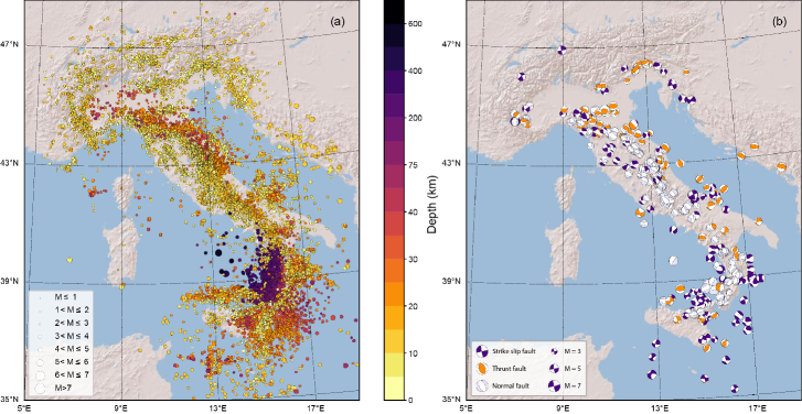
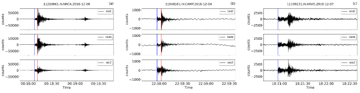
Figure 1: Top-left panel: Earthquake locations; Top-right panel: Seismic stations used for waveforms extraction. The symbol sizes are proportional to earthquake magnitude and number of arrival phases recorded by stations, respectively; Bottom panels: Seismic waveforms of some events with magnitude in the range $[2,4]$. Source: Michelini et al., (2021).

Earthquakes’ detection provides a whole set of data which are usually studied separately, i.e. spatial (and temporal) occurrence of points through point process theory (Siino et al., (2017); Iftimi et al., (2019); D’Angelo et al., 2022b , to cite just a few recent works), and the analysis of waveforms through FDA (Adelfio et al.,, 2011, 2012; Chiodi et al.,, 2013).

A recently released set of data on Italian seismic activity encompasses both of these data types. The Italian seismic dataset for machine learning (INSTANCE) is a dataset of seismic waveforms data and associated metadata (Michelini et al.,, 2021), which includes 54008 earthquakes for a total of 1159249 3-channel waveforms. It also contains 132330 3-channel noise waveforms. For each of these waveforms, 115 metadata (i.e. statistical variables) are available, providing information on station, trace, source, path and quality. Overall, the data are collected by 19 networks which consist of 620 seismic stations. The dataset is available on http://www.pi.ingv.it/instance/.

The earthquake list in the dataset is based on the Italian seismic bulletin (http://terremoti.ingv.it/bsi) of the “Istituto Nazionale di Geofisica e Vulcanologia”, includes events which occurred between January 2005 and January 2020, and in the magnitude range between 0.0 and 6.5. The waveform data have been recorded primarily by the Italian National Seismic Network. The top panels of Figure 1 depict the earthquake locations and the seismic stations which recorded the events.

In the bottom panels of Figure 1, some waveforms contained in the dataset are represented. All the waveform traces have a length of 120 seconds, are sampled at 100 Hz, and are provided both in counts and ground motion physical units after deconvolution of the instrument transfer functions. The waveform dataset is accompanied by metadata consisting of more than 100 variables providing comprehensive information on the earthquake source, the recording stations, the trace features, and other derived quantities.

3 Preliminaries on marked point processes

Throughout the paper, we consider marked point processes $Y=\{(x_{i},m_{i})\}_{i=1}^{N}$ (Daley and Vere-Jones,, 2008, Definition 6.4.1), with ground points $x_{i}$ in the $d$-dimensional Euclidean space $\mathbb{R}^{d}$, $d\geq 1$, which is equipped with the Lebesgue measure $|A|=\int_{A}\text{d}z$ for Borel sets $A\in\mathcal{B}(\mathbb{R}^{d})$; a closed Euclidean $r$-ball around $x\in\mathbb{R}^{d}$ will be denoted by $b[x,r]$. By definition, the ground process $Y_{g}=\{x_{i}\}_{i=1}^{N}$, obtained from $Y$ by ignoring the marks, is a well-defined point process on $\mathbb{R}^{d}$ in its own right. We shall assume that $Y$ is simple, that is, it almost surely (a.s.) does not contain multiple points. Note that, formally, $Y$ is a random element in the measurable space $(N_{lf},\mathcal{N})$ of locally finite point configurations/patterns $\mathbf{x}=\{((x_{1},m_{1}),\ldots,(x_{n},m_{n}))\}$, $n\geq 0$ (Daley and Vere-Jones,, 2008; Van Lieshout,, 2000). We assume that the mark space $\mathcal{M}$ is Polish and equipped with a finite reference measure $\nu$ on the Borel $\sigma$-algebra $\mathcal{B(M)}$. The Borel $\sigma$-algebra $\mathcal{B}(\mathbb{R}^{d}\times\mathcal{M})=\mathcal{B}(\mathbb{R}^{d})\otimes\mathcal{B}(\mathcal{M})$ is endowed with the product measure $A\times E\mapsto|A|\nu(E)$, $A\times E\in\mathcal{B}(\mathbb{R}^{d}\times\mathcal{M})$. We will let $Y(A\times E)=\sum_{(x,m)\in Y}\mathbf{1}\{(x,m)\in A\times E\}$, where $\mathbf{1}$ is the indicator function, denote the cardinality of the random set $Y\cap(A\times E)$.

Given this general setup, one may obtain various forms of marked point processes, most notably multivariate/multitype point processes with $\mathcal{M}=\{1,\ldots,k\}$ (Diggle,, 2013) and functional marked point processes with $\mathcal{M}$ given by a suitable function space (Ghorbani et al.,, 2021).

3.1 Functional Marked Point Processes

In this section, we provide the definition of functional marked point processes following Ghorbani et al., (2021).

In classical FDA, one analyses a collection of functions $\{f_{1}(t),\ldots,f_{n}(t)\}$, $t\in\mathcal{T}\subset[0,\infty)$, $n\geq 1$, which take values in some Euclidean space $\mathbb{R}^{k}$, $k\geq 1$, and belong to some suitable function space, typically an $L_{2}$-space. Although $t$ usually represents time, it could also represent some other quantity, for example, spatial distance. Classically, one would assume that such a collection of functions constitute realisations or samples of some collection of independent and identically distributed (iid) random functions or stochastic processes $\{F_{1}(t),\ldots,F_{n}(t)\}$, $t\in\mathcal{T}$. Such an assumption may, however, be questioned in certain settings. For example, two functions $f_{i}$ and $f_{j}$, which are spatially close to each other in $\mathbb{R}^{k}$, could gain (or lose) from being close to each other. Accordingly, it seems natural to relax the iid assumption for $F_{1},\ldots,F_{N}$. A natural way to handle such a scenario is to generate $F_{1},\ldots,F_{N}$ conditionally on some collection of (dependent) random spatial locations. Note that the conditional distribution of $F_{1},\ldots,F_{N}$ could render them both dependent and independent.

To facilitate such a setting, we consider a functional marked point process (Ghorbani et al.,, 2021), which is defined as a marked point process where the marks are random elements in some (Polish) function space, $\mathcal{M}$, most notably the space of $L_{2}$-functions $f:\mathcal{T}\to\mathbb{R}^{k}$. Realisations of FMPPs are called functional marked point patterns. It is noteworthy that the original formal construction of functional marked point processes by Ghorbani et al., (2021) also included an additional non-functional mark, so that each ground process point would be marked by a pair which consists of a function and a non-functional variable. We here do not consider such auxiliary non-functional marks.

3.2 Product densities

Provided that it exists, the $n$-th order intensity/product density function $\rho^{(n)}$, $n\geq 1$, which is the density of the $n$-th order factorial moment measure $\alpha^{(n)}$, may be specified through the $n$-th order Campbell formula. It states that, for any non-negative measurable function $h$ on $(\mathbb{R}^{d}\times\mathcal{M})^{n}$, the expectation of the random sum of $h$ over $n$-tuples of distinct points of $Y$ satisfies

$$\begin{split}&\mathbb{E}\left[\sum^{\neq}_{(x_{1},m_{1}),\ldots,(x_{n},m_{n})\in Y}h((x_{1},m_{1}),\ldots,(x_{n},m_{n}))\right]=\\ &=\int\cdots\int h((x_{1},m_{1}),\ldots,(x_{n},m_{n}))\rho^{(n)}((x_{1},m_{1}),\ldots,(x_{n},m_{n}))\prod_{i=1}^{n}\text{d}x_{i}\nu(dm_{i}).\end{split}$$ (1)

Heuristically, $\rho^{(n)}((x_{1},m_{1}),\ldots,(x_{n},m_{n}))\text{d}x_{1}\nu(dm_{1})\cdots\text{d}x_{n}\nu(dm_{n})$ gives the probability that $Y$ has points in infinitesimal neighbourhoods $d(x_{i},m_{i})\ni(x_{i},m_{i})\in\mathbb{R}^{d}\times\mathcal{M}$ with measures $\text{d}x_{i}\nu(dm_{i})$, $i=1,\ldots,n$. Moreover, we retrieve $\alpha^{(n)}((A_{1}\times E_{1})\times\cdots\times(A_{n}\times E_{n}))$, $(A_{i}\times E_{i})\in\mathcal{B}(\mathbb{R}^{d}\times\mathcal{M})$, $i=1,\ldots,n$, by letting $h$ be given by the indicator function $\mathbf{1}\{(x_{1},m_{1})\in(A_{1}\times E_{1}),\ldots,(x_{n},m_{n})\in(A_{n}\times E_{n})\}$. It further follows that

$$\rho^{(n)}((x_{1},m_{1}),\ldots,(x_{n},m_{n}))=f_{x_{1},\dots,x_{n}}(m_{1},\ldots,m_{n})\rho_{g}^{(n)}(x_{1},\ldots,x_{n}),$$

where $\rho_{g}^{(n)}$ is the $n$-th order product density of $Y_{g}$ and $f_{x_{1},\dots,x_{n}}(\cdot)$ is a conditional density function on $\mathcal{M}^{n}$ which governs the joint distribution of $n$ marks, given that their associated ground process points are given by $x_{1},\dots,x_{n}\in\mathbb{R}^{d}$. These, in turn, yield the corresponding mark distributions

$$M^{x_{1},\ldots,x_{n}}(E_{1},\ldots,E_{n})=\int_{E_{1}}\cdots\int_{E_{n}}f_{x_{1},\dots,x_{n}}(m_{1},\ldots,m_{n})\prod_{i=1}^{n}\nu(dm_{i}),$$

which govern the joint distribution on $n$ marks, given the associated ground process locations.

The intensity measure of $Y$, which coincides with the first order factorial moment measure, here satisfies

$$\alpha(A\times E)= \mathbb{E}[Y(A\times E)]=\int_{A}\int_{E}\rho(x,m)\text{d}x\nu(dm)$$

$$= \int_{A}\int_{E}f_{x}(m)\rho_{g}(x)\text{d}x\nu(dm)=\int_{A}M^{x}(E)\rho_{g}(x)\text{d}x,$$ (2)

where the first order intensity functions $\rho=\rho^{(1)}$ and $\rho_{g}=\rho_{g}^{(1)}$ are typically referred to as the intensity functions of $Y$ and $Y_{g}$. Note that $\rho$ may be viewed as a “heat map” which reflects the infinitesimal chance of having a point of $Y$ at/around an arbitrary location in $\mathbb{R}^{d}\times\mathcal{M}$. When the intensity function (of the ground process) is constant, we say that the (ground) process is homogeneous, otherwise it is called inhomogeneous.

When, conditional on the ground process, all marks have the same marginal univariate distribution, so that $M^{z}(E)=\int_{E}f_{z}(m)\text{d}\nu(dm)=\int_{E}f(m)\text{d}\nu(m)=M(E)$, we say that $X$ has a common (marginal) mark distribution. This holds e.g. when $Y$ is stationary, i.e. when its distribution is invariant under translations of the ground points; here $\alpha(A\times E)=\rho_{g}M(E)|A|$ and $\rho_{g}>0$ is the constant intensity of the ground process. We will see that, at times, it is particularly convenient to have here that the reference measure $\nu$ coincides with the common mark distribution $M$, which implies that the common mark density $f$ is set to $1$ and $\rho(x,m)=\rho_{g}(x)$.

When $Y$ is independently marked, i.e. when the marks are independent conditional on the ground process, $f_{x_{1},\ldots,x_{n}}(m_{1},\ldots,m_{n})=f_{x_{1}}(m_{1})\cdots f_{x_{n}}(m_{n})$ for any $n\geq 1$ and if, in addition, there is a common mark distribution, whereby the marks are iid conditional on the ground process, we say that $Y$ is randomly labelled and note that $f_{x_{1},\ldots,x_{n}}(m_{1},\ldots,m_{n})=f(m_{1})\cdots f(m_{n})$.

3.2.1 Intensity reweighted stationarity

We next turn to the notion of a $k$-th order marked intensity reweighted stationary ($k$-MIRS) marked point process $Y$ (Ghorbani et al.,, 2021). We say that $Y$ is $k$-MIRS, $k\in\{1,2,\ldots\}$, if $\rho$ is bounded away from 0 and the correlation functions

$$g^{(n)}((x_{1},m_{1}),\ldots,(x_{n},m_{n}))=$$

$$= \frac{\rho^{(n)}((x_{1},m_{1}),\ldots,(x_{n},m_{n}))}{\rho(x_{1},m_{1})\cdots\rho(x_{n},m_{n})}=\frac{f_{x_{1},\dots,x_{n}}(m_{1},\ldots,m_{n})}{f_{x_{1}}(m_{1})\cdots f_{x_{n}}(m_{n})}\frac{\rho_{g}^{(n)}(x_{1},\ldots,x_{n})}{\rho_{g}(x_{1})\cdots\rho_{g}(x_{n})},\quad n\geq 1,$$

satisfy $g^{(n)}((x_{1},m_{1}),\ldots,(x_{n},m_{n}))=g^{(n)}((z+x_{1},m_{1}),\ldots,(z+x_{n},m_{n}))$ for any $z\in\mathbb{R}^{d}$ and any $n\leq k$. Note that $g^{(1)}(\cdot)\equiv 1$ and that the second ratio on the right hand side is the $n$-th order correlation function, $g_{g}^{(n)}$, of the ground process. Provided that the product densities of all orders exist, stationarity implies $k$-MIRS for all orders $k\geq 1$. Note further that $g^{(n)}(\cdot)\equiv 1$, $n\geq 1$, for a Poisson process and when $g^{(n)}((x_{1},m_{1}),\ldots,(x_{n},m_{n}))>1$ points of $Y_{g}$ in infinitesimal neighbourhoods of $x_{1},\ldots,x_{n}$ with marks in infinitesimal neighbourhoods of $m_{1},\ldots,m_{n}$ tend to cluster/aggregate. Similarly, $g^{(n)}((x_{1},m_{1}),\ldots,(x_{n},m_{n}))<1$ indicates inhibition/regularity.

3.3 Palm distributions

Let $Y$ be a simple marked point process whose intensity function exists. Many of the summary statistics we will consider can be expressed in terms of reduced Palm distributions. These satisfy the reduced Campbell–Mecke formula which states that, for any non-negative measurable function $h$ on the product space $(\mathbb{R}^{d}\times\mathcal{M})\times N_{lf}$,

$$\mathbb{E}\left[\sum_{(z,m)\in Y}h((z,m),Y\backslash\{(z,m)\})\right]= \int\mathbb{E}[h((x,m),Y^{!(x,m)})]\rho(x,m)\text{d}x\nu(dm)$$ (3)

$$= \int\mathbb{E}^{!(x,m)}[h((x,m),Y)]\rho(x,m)\text{d}x\nu(dm).$$

Here $Y^{!(x,m)}$ is the reduced Palm process at $(x,m)\in\mathbb{R}^{d}\times\mathcal{M}$, which we interpret as $Y$ conditioned on the null event that there is a point in $(x,m)$, which is removed upon realisation. The probability distribution $P^{!(x,m)}(\cdot)=\mathbb{P}^{!(x,m)}(Y\in\cdot)=\mathbb{P}(Y^{!(x,m)}\in\cdot)$ on $(N_{lf},\mathcal{N})$, which corresponds to $\mathbb{E}^{!(x,m)}$, is called the reduced Palm distribution at $(x,m)$.

4 Local weighted marked summary statistics

Global summary statistics have had a prominent role in the statistical analysis of point processes. More precisely, their non-parametric estimators are typically used to characterise the degree of spatial interaction present in the underlying data-generating point process. In Section 1, we have reviewed a few such examples, for instance $K$-functions.

The individual contributions to a global statistic, which are commonly called Local Indicators of Spatial Association (LISA) functions, can be used to identify outlying components measuring the influence of each contribution to the global statistic (Anselin,, 1995). This is the case of the scatter plot based on the local Moran index (Anselin,, 1996). On the other hand, the individual contributions can be used to test for specific local structures, such as spatial association and hot spot detection in areal data (Getis and Ord,, 1992). Basically, the local statistics mentioned so far are often used to analyse areal data but Getis and Franklin, (1987) introduced a local version of the $K$-function for spatial point processes to show that trees exhibit different kinds of heterogeneity when examined at different scales of analysis. The notion of individual functions for certain statistics has also been studied in Stoyan and Stoyan, (1994) and Mateu et al., (2010) showed that the local product density function (Cressie and Collins,, 2001) is more sensitive to identifying different local structures and unusual points than the local $K$-function. Applications of LISA functions range from detection of features in images with noise (Mateu et al.,, 2007) to detection of disease clusters (Moraga and Montes,, 2011). In Siino et al., (2018) the authors extend local indicators of spatial association to the spatio-temporal context (LISTA functions) based on the second order product density, and these local functions have been used to define a proper statistical test for clustering detection. Recently, LISTA functions have been used both for diagnostic (Adelfio et al.,, 2020) and fitting purposes (D’Angelo et al., 2022a, ). Finally, D’Angelo et al., (2021) extended LISTA functions to spatio-temporal point processes living on linear networks.

As we have clearly indicated, an alternative to studying the aforementioned global summary statistics for marked point processes is considering local summary statistics which describe the spatial interaction in the vicinity of a given marked point. In order to do so here in the marked context, we introduce the function

$$L((x,m),\mathbf{x})=L_{n}((x,m),\mathbf{x};\tilde{t},\tilde{\rho})=\sum_{(x_{1},m_{1}),\ldots,(x_{n-1},m_{n-1})\in\mathbf{x}}^{\neq}\frac{\tilde{t}((x,m),(x_{1},m_{1}),\ldots,(x_{n-1},m_{n-1}))}{\tilde{\rho}(x,m)\tilde{\rho}(x_{1},m_{1})\cdots\tilde{\rho}(x_{n-1},m_{n-1})},$$ (4)

for $(x,m)\in\mathbb{R}^{d}\times\mathcal{M}$, point patterns $\mathbf{x}\in N_{lf}$ and measurable $\tilde{t}:(\mathbb{R}^{d}\times\mathcal{M})^{n}\to\mathbb{R}$, $n\geq 2$. Note that, formally, the argument $\tilde{\rho}$ does not need to be the true intensity function $\rho$ of $Y$, it could e.g. be a plug-in estimator. We will exploit Definition 1, and thereby (4), to define proper notions of (mark-weighted $n$-th order inhomogeneous) local summary statistics.

Definition 1.

Given a marked point process $Y$, we refer to $L((x,m),Y\setminus\{(x,m)\};\tilde{t},\tilde{\rho})$, $(x,m)\in Y$, as the family of $n$-th order local marked cumulative summary statistics of $Y$ associated with $\tilde{t}$ and $\tilde{\rho}$.

The construction of a specific local statistic is obtained by identifying when, for some function family $\{\tilde{t}_{r}\}$,

$$G(r,Y)=\sum_{(x,m)\in Y}L_{n}((x,m),Y\setminus\{(x,m)\};\tilde{t}_{r},\tilde{\rho})$$ (5)

forms an estimator of an existing global summary statistic.

Using $n$-th order local marked cumulative summary statistics to quantify local spatial interactions for a point pattern $\mathbf{x}$ entails inserting an estimate $\widehat{\rho}(x,m)=\widehat{f}_{z}(m)\widehat{\rho}_{g}(x)$ for the unknown intensity $\rho(x,m)=f_{z}(m)\rho_{g}(x)$, i.e. setting $\tilde{\rho}=\widehat{\rho}$. When we assume that there is a common mark distribution which coincides with the mark reference measure $\nu$, we obtain that $\widehat{\rho}(x,m)=\widehat{\rho}_{g}(x)$, i.e. the intensity estimate does not depend on the mark values. Imposing this assumption is particularly convenient when dealing with functional marks since estimation of the mark density, which here is a density on a function space, is rather challenging and beyond the scope of this paper. Note that when $Y$ is randomly labelled, it has a common mark distribution and in this setting the assumption $\widehat{\rho}(x,m)=\widehat{\rho}_{g}(x)$ thus makes sense.

Turning to the distributional properties of the $n$-th order local marked cumulative summary statistics, we next derive their expectations under the assumption of $k$-MIRS. Note, in particular, that the choice of $\tilde{t}$ plays a significant role here.

Theorem 1.

When $Y$ is $k$-MIRS and $\tilde{\rho}=\rho$, for any $W\in\mathcal{B}(\mathbb{R}^{d})$ the expectation of $L((x,m),Y\setminus\{(x,m)\}\cap W\times\mathcal{M};\tilde{t},\rho)$, $(x,m)\in Y\cap W\times\mathcal{M}$, is almost everywhere given by

$$\int_{W-x}\cdots\int_{W-x}\Bigg{(}\int_{\mathcal{M}}\cdots\int_{\mathcal{M}}\tilde{t}((x,m),(x_{1}+x,m_{1}),\ldots,(x_{n-1}+x,m_{n-1}))\times$$

$$\times\frac{f_{0,x_{1},\ldots,x_{n-1}}(m,m_{1},\ldots,m_{n-1})}{f_{0}(m)f_{x_{1}}(m_{1})\cdots f_{x_{n-1}}(m_{n-1})}\nu(dm_{1})\cdots\nu(dm_{n-1})\Bigg{)}g_{g}^{(n)}(0,x_{1},\ldots,x_{n-1})\text{d}x_{1}\cdots\text{d}x_{n-1},$$

when $2\leq n\leq k$. Moreover, the expectation of $G(r,Y\cap W\times\mathcal{M})$ is obtained by replacing $\tilde{t}$ by $\tilde{t}_{r}$ in the expression above and integrating it over $W\times\mathcal{M}$ with respect to the reference measure on $\mathbb{R}^{d}\times\mathcal{M}$.

Proof.

Note first that the expectation coincides with

$$\mathbb{E}^{!(x,m)}[L_{n}((x,m),Y\cap W\times\mathcal{M};\tilde{t},\rho)]=$$

$$= \mathbb{E}^{!(x,m)}\left[\sum_{(x_{1},m_{1}),\ldots,(x_{n-1},m_{n-1})\in Y\cap W\times\mathcal{M}}^{\neq}\frac{\tilde{t}((x,m),(x_{1},m_{1}),\ldots,(x_{n-1},m_{n-1}))}{\rho(x,m)\rho(x_{1},m_{1})\cdots\rho(x_{n-1},m_{n-1})}\right].$$

Hence, our starting point will be the reduced Campbell-Mecke formula. Consider an arbitrary bounded $A\times E\in\mathcal{B}(\mathbb{R}^{d}\times\mathcal{M})$. It follows that

$$\mathbb{E}\left[\sum_{(x,m)\in Y\cap A\times E}\sum_{(x_{1},m_{1}),\ldots,(x_{n-1},m_{n-1})\in Y\setminus\{(x,m)\}\cap W\times\mathcal{M}}^{\neq}\frac{\tilde{t}((x,m),(x_{1},m_{1}),\ldots,(x_{n-1},m_{n-1}))}{\rho(x,m)\rho(x_{1},m_{1})\cdots\rho(x_{n-1},m_{n-1})}\right]=$$

$$= \int_{A\times E}\mathbb{E}^{!(x,m)}\left[\sum_{(x_{1},m_{1}),\ldots,(x_{n-1},m_{n-1})\in Y\cap W\times\mathcal{M}}^{\neq}\frac{\tilde{t}((x,m),(x_{1},m_{1}),\ldots,(x_{n-1},m_{n-1}))}{\rho(x_{1},m_{1})\cdots\rho(x_{n-1},m_{n-1})}\right]\text{d}x\nu(dm).$$

On the other hand, by the Campbell formula we have that

$$\mathbb{E}\left[\sum_{(x,m)\in Y\cap A\times E}\sum_{(x_{1},m_{1}),\ldots,(x_{n-1},m_{n-1})\in Y\setminus\{(x,m)\}\cap W\times\mathcal{M}}^{\neq}\frac{\tilde{t}((x,m),(x_{1},m_{1}),\ldots,(x_{n-1},m_{n-1}))}{\rho(x,m)\rho(x_{1},m_{1})\cdots\rho(x_{n-1},m_{n-1})}\right]=$$

$$= \int_{A\times E}\int_{\mathbb{R}^{d}\times\mathcal{M}}\cdots\int_{\mathbb{R}^{d}\times\mathcal{M}}\mathbf{1}\{x_{1},\ldots,x_{n-1}\in W\}\tilde{t}((x,m),(x_{1},m_{1}),\ldots,(x_{n-1},m_{n-1}))\times$$

$$\times g^{(n)}((x,m),(x_{1},m_{1}),\ldots,(x_{n-1},m_{n-1}))\text{d}x_{1}\nu(dm_{1})\cdots\text{d}x_{n-1}\nu(dm_{n-1})\text{d}x\nu(dm)$$

$$= \int_{A\times E}\int_{\mathbb{R}^{d}\times\mathcal{M}}\cdots\int_{\mathbb{R}^{d}\times\mathcal{M}}\prod_{i=1}^{n-1}\mathbf{1}\{u_{i}\in W-x\}\tilde{t}((x,m),(u_{1}+x,m_{1}),\ldots,(u_{n-1}+x,m_{n-1}))\times$$

$$\times g^{(n)}((0,m),(u_{1},m_{1}),\ldots,(u_{n-1},m_{n-1}))\text{d}u_{1}\nu(dm_{1})\cdots\text{d}u_{n-1}\nu(dm_{n-1})\text{d}x\nu(dm)$$

by the imposed $k$-MIRS and a change of variables, $u_{i}+x=x_{i}$. Hence, since $A\times E\in\mathcal{B}(\mathbb{R}^{d}\times\mathcal{M})$ was arbitrary, for almost every $(x,m)$ we have that

$$\mathbb{E}^{!(x,m)}[L_{n}((x,m),Y;\tilde{t},\rho)]=$$

$$= \int_{(W-x)\times\mathcal{M}}\cdots\int_{(W-x)\times\mathcal{M}}\tilde{t}((x,m),(u_{1}+x,m_{1}),\ldots,(u_{n-1}+x,m_{n-1}))\times$$

$$\times g^{(n)}((0,m),(u_{1},m_{1}),\ldots,(u_{n-1},m_{n-1}))\text{d}u_{1}\nu(dm_{1})\cdots\text{d}u_{n-1}\nu(dm_{n-1})$$

$$= \int_{W-x}\cdots\int_{W-x}\Bigg{(}\int_{\mathcal{M}}\cdots\int_{\mathcal{M}}\tilde{t}((x,m),(u_{1}+x,m_{1}),\ldots,(u_{n-1}+x,m_{n-1}))\times$$

$$\times\frac{f_{0,u_{1},\ldots,u_{n-1}}(m,m_{1},\ldots,m_{n-1})}{f_{0}(m)f_{u_{1}}(m_{1})\cdots f_{u_{n-1}}(m_{n-1})}\nu(dm_{1})\cdots\nu(dm_{n-1})\Bigg{)}g_{g}^{(n)}(0,u_{1},\cdots,u_{n-1})\text{d}u_{1}\cdots\text{d}u_{n-1},$$

by Fubini’s theorem.

∎

The first thing we note is that when $Y$ is independently marked then the density ratio in the expression for the expectation vanishes. In addition, if $Y$ is a Poisson process on $\mathbb{R}^{d}\times\mathcal{M}$ which satisfies being a marked point process with mark space $\mathcal{M}$, then the expectation reduces to an integral with $\tilde{t}$ as integrand. These observations may be used as benchmarks for when $Y$ exhibits mark (in)dependence and spatial interaction locally.

4.1 Special cases

We next illustrate how (5), through Definition 1 and (4), reduces to several existing summary statistic estimators by varying $\tilde{t}$ and $\tilde{\rho}$.

4.1.1 Ground K-functions

First, set $n=2$ and $\tilde{t}$ to $\tilde{t}_{r}((x,m),(x_{1},m_{1}))=w(x,x_{1})\mathbf{1}\{x_{1}\in x+C\}/|W|$, $r\geq 0$, where $W\subseteq\mathbb{R}^{d}$, $|W|>0$, and $w(\cdot)$ is an edge correction term. If the ground process is stationary with intensity $\rho_{g}>0$ and $\tilde{\rho}(x,m)\equiv\rho_{g}$, then (5) with $Y$ set to $Y\cap W\times\mathcal{M}$ reduces to an estimator of Ripley’s $K$-function when $x+C=x+b[0,r]=b[x,r]$ whereas if the ground process is inhomogeneous and we set $\tilde{\rho}(x,m)=\rho_{g}(x)$, it follows that (5) reduces to an estimator of the inhomogeneous $K$-function (Baddeley et al.,, 2000) for $Y_{g}$. The extension to space-time is straightforward; replace the Euclidean ball $b[0,r]$ by $C=\{(x,s):\|x\|\leq r,|s|\leq t\}\in\mathcal{B}(\mathbb{R}^{d+1})$, where $\|\cdot\|$ denotes the Euclidean norm (Cronie and Van Lieshout,, 2015; Gabriel and Diggle,, 2009; Iftimi et al.,, 2019).

4.1.2 Marked K-functions

When $n=2$, by instead letting $\tilde{t}_{r}((x,m),(x_{1},m_{1}))=w(x,x_{1})\mathbf{1}\{x_{1}\in x+C\}\mathbf{1}\{m\in E,m_{1}\in E_{1}\}/(|W|\nu(E)\nu(E_{1}))$ and $\tilde{\rho}=\rho$ in (4), using a suitable edge correction function $w(\cdot)$, then $G(r,Y\cap W\times\mathcal{M})$ in (5) reduces to an estimator of the marked second order reduced moment measure $\mathcal{K}^{EE_{1}}(C)$ of Iftimi et al., (2019), which measures the intensity reweighted interactions between points with marks in $E$ and points with marks in $E_{1}$, when their separation vectors belong to $C\in\mathcal{B}(\mathbb{R}^{d})$. We note that measures of this kind are in general not symmetric, i.e.  $\mathcal{K}^{EE_{1}}(\cdot)\neq\mathcal{K}^{E_{1}E}(\cdot)$ (Iftimi et al.,, 2019). Furthermore, choosing $C$ to be the closed origin-centred ball $b[0,r]$ of radius $r\geq 0$, we consider the marked inhomogeneous $K$-function $K^{EE_{1}}_{inhom}(r)$ of Cronie and van Lieshout, (2016), which measures pairwise intensity reweighted spatial dependence within distance $r$ between points with marks in $E$ and points with marks in $E_{1}$.

By additionally letting $n>2$, we obtain a definition of a marked $n$-th order reduced moment measure, $\mathcal{K}^{E\times_{i=1}^{n-1}E_{i}}(C_{1}\times\cdots\times C_{n-1})$, which measures the intensity reweighted spatial interaction between an arbitrary point with mark in $E$ and distinct $(n-1)$-tuples of other points, where the separation vectors between the $E$-marked point and these $n-1$ points, which have marks in $E_{1},\ldots,E_{n-1}$, belong to $C_{1},\ldots,C_{n-1}$. We note that $C_{i}=b[0,r]$, $i=1,\ldots,n-1$, $r\geq 0$, yields an $n$-point version of the marked inhomogeneous $K$-function $K_{inhom}^{E\times_{i=1}^{n-1}E_{i}}(r)$ of Cronie and van Lieshout, (2016), which may be used to analyse intensity reweighted interactions between a point with mark in $E$ and $n-1$ of its $r$-close neighbours, which have marks belonging to the respective sets $E_{1},\ldots,E_{n-1}$.

4.1.3 Weighted marked reduced moment measures and K-functions

Finally, by letting $\tilde{\rho}=\rho$ and $\tilde{t}((x,m),(x_{1},m_{1}),\ldots,(x_{n-1},m_{n-1}))$ be given by the product of

$$\tilde{t}(m,m_{1},\ldots,m_{n-1})= t(m,m_{1},\ldots,m_{n-1})\frac{\mathbf{1}\{m\in E\}}{\nu(E)}\prod_{i=1}^{n-1}\frac{\mathbf{1}\{m_{i}\in E_{i}\}}{\nu(E_{i})},$$ (6)

$$\tilde{w}(x,x_{1},\ldots,x_{n-1})= w(x,x_{1},\ldots,x_{n-1})\prod_{i=1}^{n-1}\mathbf{1}\{x_{i}\in(x+C_{i})\},$$

for $E\in\mathcal{B(M)}$, $\nu(E)>0$, and $C_{i}\times E_{i}\in\mathcal{B}(\mathbb{R}^{d})\times\mathcal{B(M)}=\mathcal{B}(\mathbb{R}^{d}\times\mathcal{M})$, $\nu(E_{i})>0$, $i=1,\ldots,n-1$, we obtain an unbiased estimator $\hat{\mathcal{K}}_{t}^{E\times_{i=1}^{n-1}E_{i}}(C_{1}\times\cdots\times C_{n-1})=G(r,Y\cap W\times\mathcal{M})$ of the $t$-weighted marked $n$-th order reduced moment measure of Ghorbani et al., (2021),

$$\mathcal{K}_{t}^{E\times_{i=1}^{n-1}E_{i}}(C_{1}\times\cdots\times C_{n-1})=$$ (7)

$$= \frac{1}{|W|\nu(E)\prod_{i=1}^{n-1}\nu(E_{i})}\mathbb{E}\Bigg{[}\sum_{(x,m)\in Y\cap W\times E}\sum_{(x_{1},m_{1}),\ldots,(x_{n-1},m_{n-1})\in Y\setminus\{(x,m)\}}^{\neq}\frac{t(m,m_{1},\ldots,m_{n-1})}{\rho(x,m)}\times$$

$$\times\prod_{i=1}^{n-1}\frac{\mathbf{1}\{x_{i}-x\in C_{i}\}\mathbf{1}\{m_{i}\in E_{i}\}}{\rho(x_{i},m_{i})}\Bigg{]}$$

assuming that the edge correction function $w$ is such that unbiasedness holds. Examples of such $w$ include the minus sampling edge correction and the translational edge correction (Ghorbani et al.,, 2021). Note here that one just as well could have merged the scaled indicators in the expression for $\tilde{t}$ with $t$ so that $\tilde{t}=t$; Ghorbani et al., (2021) included this mark set filtering to highlight that their summary statistic generalises previously proposed ones.

4.2 Local t-weighted marked $n$-th order inhomogeneous K-function

In this section, we provide the estimator corresponding to the local contributions of (7) and discuss its properties.

Definition 2.

Let $\tilde{t}$ be (up to indicator-scaling) as in (6) and consider

$$\begin{split}&\hat{\mathcal{K}}_{t}^{(x,m)\times_{i=1}^{n-1}E_{i}}(C_{1}\times\cdots\times C_{n-1})=L_{n}((x,m),Y\setminus\{(x,m)\}\cap W\times\mathcal{M};\tilde{t},\tilde{\rho})=\\ =&\frac{1}{\tilde{\rho}(x,m)\nu(E)\prod_{i=1}^{n-1}\nu(E_{i})}\sum_{(x_{1},m_{1}),\ldots,(x_{n-1},m_{n-1})\in Y\setminus\{(x,m)\}\cap W\times\mathcal{M}}^{\neq}w(x,x_{1},\ldots,x_{n-1})\times\\ &\times t(m,m_{1},\ldots,m_{n-1})\prod_{i=1}^{n-1}\frac{\mathbf{1}\{x_{i}-x\in C_{i}\}\mathbf{1}\{m_{i}\in E_{i}\}}{\tilde{\rho}(x_{i},m_{i})},\qquad(x,m)\in Y\cap W\times\mathcal{M},\end{split}$$ (8)

for some suitable edge correction $w$ in (6), $W\in\mathcal{B}(\mathbb{R}^{d})$, $E\in\mathcal{B}(\mathcal{M})$, $\nu(E)>0$, and $C_{i}\times E_{i}\in\mathcal{B}(\mathbb{R}^{d}\times\mathcal{M})$, $\nu(E_{i})>0$, $i=1,\ldots,n-1$. We refer to $\hat{\mathcal{K}}_{t}^{(x,m)\times_{i=1}^{n-1}E_{i}}(r)=\hat{\mathcal{K}}_{t}^{(x,m)\times_{i=1}^{n-1}E_{i}}(b[0,r]^{n-1})$, $r\geq 0$, as a local t-weighted marked $n$-th order inhomogeneous $K$-function. In particular, $\hat{\mathcal{K}}_{t,n}^{(x,m)}(r)=\hat{\mathcal{K}}_{t}^{(x,m)\times\mathcal{M}^{n-1}}(r)$ does not perform any explicit mark set filtering.

Note first that when there is a common mark distribution which coincides with the reference measure on $\mathcal{M}$, setting $\tilde{\rho}=\rho$ we, for instance, obtain

$$\hat{\mathcal{K}}_{t,n}^{(x,m)}(r)= \sum_{(x_{1},m_{1}),\ldots,(x_{n-1},m_{n-1})\in Y\setminus\{(x,m)\}\cap(b[x,r]\cap W)\times\mathcal{M}}^{\neq}\frac{t(m,m_{1},\ldots,m_{n-1})w(x,x_{1},\ldots,x_{n-1})}{\rho_{g}(x)\rho_{g}(x_{1})\cdots\rho_{g}(x_{n-1})}$$

since $\nu$ must be a probability measure here.

Regarding the distributional properties of (8), when $Y$ is $k$-MIRS, Theorem 1 tells us that the expectation is given by

$$\frac{1}{\nu(E)}\prod_{i=1}^{n-1}\frac{1}{\nu(E_{i})}\int_{\mathbb{R}^{d}}\cdots\int_{\mathbb{R}^{d}}w(x,x_{1}+x,\ldots,x_{n-1}+x)\prod_{i=1}^{n-1}\mathbf{1}\{x_{i}\in(x+C_{i})\cap(W-x)\}\times$$

$$\times \Bigg{(}\int_{E_{1}}\cdots\int_{E_{n-1}}t(m,m_{1},\ldots,m_{n-1})\frac{f_{0,x_{1},\ldots,x_{n-1}}(m,m_{1},\ldots,m_{n-1})}{f_{0}(m)f_{x_{1}}(m_{1})\cdots f_{x_{n-1}}(m_{n-1})}\nu(dm_{1})\cdots\nu(dm_{n-1})\Bigg{)}\times$$

$$\times g_{g}^{(n)}(0,x_{1},\ldots,x_{n-1})\text{d}x_{1}\cdots\text{d}x_{n-1}.$$

In particular, under independent marking the mark related integral within brackets reduces to $\int_{E_{1}}\cdots\int_{E_{n-1}}t(m,m_{1},\ldots,m_{n-1})\nu(dm_{1})\cdots\nu(dm_{n-1})$, whereby (8) is given by the product of this term and a term measuring intensity reweighted spatial interaction.

4.2.1 Test functions for FMPPs

Turning to the FMPP case, by choosing different test functions $t(\cdot)$ for the functional marks, we may extract different features. We here focus on pairwise interactions, i.e. $n=2$.

The test function $t$ is intended to reflect similarities between functions. Hence, a natural starting point would be a metric $t(f_{1},f_{2})=d(f_{1},f_{2})$ on the function space $\mathcal{M}$, which does not necessarily need to be the underlying assumed metric on $\mathcal{M}$. The first candidate that comes to mind is an $L_{p}$-distance:

$$t(f_{1},f_{2})=\Bigg{(}\int_{a}^{b}|f_{1}(t)-f_{2}(t)|^{p}\text{d}t\Bigg{)}^{1/p},\quad 1\leq p\leq\infty,$$ (9)

where $p=\infty$ represents the supremum metric. For any choice of $p$ in (9), similarity between functions implies a small value of the test function. Other tentative functions are semi-metrics based on the $L_{p}$ distance between the $s$-th derivatives of the functions, for different combinations of $p$ and $s$, with the $L_{1}$ and $L_{2}$ distances being particular cases, and semi-metrics based on functional principal component analysis.

A further alternative is the functional marked counterpart of the test function for the classical variogram, given by

$$t(f_{1},f_{2})=\int_{a}^{b}(f_{1}(t)-\bar{F}(t))(f_{2}(t)-\bar{F}(t))\text{d}t,$$ (10)

with $\bar{F}(t)=(1/n)\sum_{i=1}^{n}f_{i}(t)$ being the average functional mark at time $t$ for the observed functional part of the point pattern; such averaging is motivated by the assumption of a common mark distribution.

5 Local test for random labelling

Simple hypotheses for spatial point patterns, such as Complete Spatial Randomness, are commonly tested using an estimator of a global summary statistic, e.g., Ripley’s $K$-function. In this context, one typically resorts to Monte Carlo testing. The first step is then to generate $Q$ simulations under the null hypothesis, and to estimate the chosen summary statistic for both the observed pattern and the simulations. In order to study whether there is random labelling in a (functional) marked point process, the simulations are obtained by permuting the (functional) marks, that is, randomly assigning them to the spatial points of the ground pattern, which are kept fixed. Then, the chosen summary statistic is estimated for each of these permutations and global envelopes at a given nominal level are generated based on them. The result of the test can be assessed graphically: if the summary statistic estimate for the observed pattern exits the envelopes, we proceed with the assumption that the underlying FMPP is not randomly labelled. Furthermore, it is possible to calculate a $p$-value based on the position of the observed summary statistic within the $q$th envelopes, following Myllymäki et al., (2017). We know, however, that the conclusion drawn from the application of the above-mentioned global test pertains to the whole analysed process, indicating whether all the functional marks are randomly labelled or not. Motivated by the will to further detect the specific points, and regions, where the functional marks really do depend on the other marked points, we propose a local test for random labelling. The main idea is to run a global envelope test on each point of the analysed pattern by means of the previously proposed local t-weighted marked inhomogeneous $K$-functions, to draw different conclusions about the individual points, based on the obtained $p$-values. In Algorithm 1 we outline the proposed local test. Note that we alternatively may use sampling without replacement in step 5 of Algorithm 1. Moreover, if convinced that multiple testing issues are present here, one may adjust the type I error probability $\alpha$ by using e.g. the Holm-Bonferroni method.

Algorithm 1 Local test of random labelling

1:Set a fixed nominal value $\alpha$ for type I error;

2:Consider a (functional) marked point pattern $\mathbf{x}=\{(x_{j},m_{j})\}_{j=1}^{k}$, $k\geq 1$;

3:Set a number of simulations, $Q\geq 1$;

4:for each $q=1,\ldots,Q$: do

5:      Randomly sample $k$ (functional) marks, with replacement, from the original $k$ ones;

6:     Denote the resulting point pattern by $\mathbf{x}_{q}=\{(x_{j},m_{j}^{q})\}_{j=1}^{k}$;

7:end for

8:for each $j=1,\ldots,k$, do

9:     Compute $L_{n}^{(j,q)}=\{\hat{\mathcal{K}}_{t}^{(x_{j},m_{j}^{q})\times_{i=1}^{n-1}E_{i}}(r;\mathbf{x}_{q})\}_{r\in[0,r_{max}]}$ for all $q=1,\ldots,Q$;

10:     Apply global envelope testing, using the functions $L_{n}^{(j,q)}$, $q=1,\ldots,Q$, to generate the envelopes;

11:     Obtain a $p$-value $p_{j}$ from the test;

12:      Reject the null hypothesis for the $j^{th}$ point if $p_{j}\leq\alpha$.

13:end for

6 Motivating example and simulation study

This section is dedicated to simulation studies to assess the performance of our proposed local test. First, section 6.1 provides a motivating example of the use of such a test, by means of simulated data resembling seismic events, which in turn have motivated this work. In particular, this means simulating the functional marks as seismic waveforms, following the typical abrupt change in variance of the signal in correspondence with the arrivals of the first P- and S-waves. Then, section 6.2 presents an extensive simulation study, showing diverse and more general settings. Specifically, we assess the performance of the test by summarising the results in terms of classification rates.

6.1 The need for a local test

We simulate a homogeneous spatial point pattern with 250 points on the unit square, $W=[0,1]\times[0,1]$, which represents the ground pattern. For each ground point $x_{i}$, we simulate a functional mark of the from

$$f_{i}(t)= y(t)=\mu(t)+\epsilon(t),\qquad t\in\mathcal{T}=[0,1],$$

$$\epsilon(t)\sim N(0,\sigma(t)^{2}),$$

$$\sigma(t)^{2}= 0.2+7.5\mathbf{1}\{t>0.4\}-5\mathbf{1}\{t>0.6\},$$

where the mean signal $\mu(t)$ is taken to be zero. The spatial ground point pattern and the corresponding waveform for a given point are shown in Figure 2(a)-(b). Since the marks/waveforms are simulated from the same model, and independently of each other and the spatial locations of the points, we see that such a process is indeed random labelled.

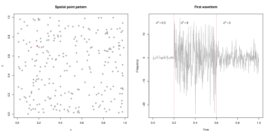
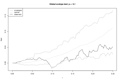
Figure 2: Simulated earthquake locations (a); Simulated waveform attached to the red point on the left (b); Result of global test (c).

Having generated the data, we first run a global envelope test for random labelling, by randomly permuting the simulated waveforms, i.e. the functional marks, keeping the location of the points fixed. We run the test by means of the t-weighted marked $n$-th order inhomogeneous $K$-function of Ghorbani et al., (2021), with $n=2$, making it a second order summary statistic, and $t$ given by the test function (10), i.e. the functional marked counterpart of the test function for the classical variogram. As previously mentioned, we assume that there is a common mark distribution which coincides with the reference measure on the mark space so that the intensity function is estimated by the ground process intensity estimate. To be as objective as possible, we do not use the homogeneous intensity estimator $\widehat{\rho}_{g}(\cdot)=Y_{g}(W)/|W|$ here but instead we use a kernel intensity estimator, as in practice it would be unknown to us whether the actual ground process is (in)homogeneous. We use a Gaussian kernel intensity estimator $\widehat{\rho}_{g}(\cdot)$, where we select the bandwidth, $h$, according to Cronie and Van Lieshout, (2018). More specifically, we minimise the discrepancy between the area of the observation window and the sum of reciprocal estimated intensity values at the points of the point pattern, i.e. we minimise $CvL(h)=(|W|-\sum_{i}1/\hat{\rho}_{g}(x_{i};h))^{2}$, where the sum is taken over all the data points $x_{i}$ and $\hat{\rho}_{g}(x_{i};h)$ is the kernel intensity estimate with bandwidth $h$, evaluated in $x_{i}$. Then, once the bandwidth has been selected, the intensity estimate is corrected for edge effects through global edge correction (the option diggle=FALSE in the spatstat function density.ppp), i.e. dividing the estimate by the convolution of the Gaussian kernel with the window of observation (Diggle,, 1985). Finally, for $w$ we use Ripley’s isotropic edge correction in the summary statistic to correct for edge effects. We repeated the procedure $39$ times, obtaining the result depicted in Figure 2(c). We stress that our approach seems to be robust with respect to the bandwidth specification, i.e. the choice of bandwidth selection approach plays a minor role for the final result.

As evident from Figure 2(c), the observed summary statistic completely lies within the envelopes, and this confirms the expected result of lack of spatial dependence/structure of the functional marks. This result is further corroborated by the non-significant $p$-value, equal to $0.1$.

6.1.1 Simulating spatially dependent functional marks

To make the functional marks spatially dependent, we then superimpose a homogeneous spatial point pattern with $50$ points, generated in the $[0,0.5]\times[0,0.5]$ square, i.e. the bottom left region of the entire study region $W$. For these additional points, we generate different functional marks than before, namely with the underlying trend $\mu(t)=10+6\sin(3\pi z_{t})$. Consequently, we have simulated a FMPP with spatially varying functional marks, i.e. not random labelled. We therefore expect a global test of random labelling to confirm this.

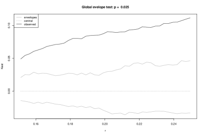
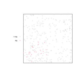
Figure 3: Result of global test for the spatially dependent simulated data (a); Output of the local test: significant points for which the hypothesis of random labelling is rejected are in pink (b).

We first run the same global test of random labelling as before. We use $Q=39$ and obtain a global $p$-value of $0.025$. This, together with the observed $K$-function lying outside the envelopes (Figure 3(a)), indicates the ability of the global test to correctly detect the spatial dependence of the functional marks.

We know, however, that this conclusion should not be drawn for each point of the pattern, if we consider local restrictions of it, but specifically for those in the vicinity of the $[0,0.5]\times[0,0.5]$ square. We therefore proceed by running our proposed local test, based on the proposed second order local $K$-function $\hat{\mathcal{K}}_{t,2}^{(x,m)}(r)$, $r\in[0,r_{max}]$, in Definition (2), with the same choice of test function $t(\cdot)$ and the same intensity estimation scheme as for the global one. Figure 3(b) depicts the points of the simulated point pattern, and it displays in pink those points for which the local test came out significant. Hence, this illustrates that the proposed local test is able to correctly identify some of the points, and consequently some parts of the region, where the hypothesis of random labelling does not hold locally. Note that a universally preferable option for $r_{max}$ does not exist. In this paper, it is set to $\min(x_{W},y_{W})/4$, where $x_{W}$ and $y_{W}$ represent the maximum width and height of the observation region $W$, respectively; note that this rule of thumb is supported by Diggle, (2013). Indeed, changing the value of $r_{max}$ has an impact on the final results, and we found that our choice provided the best compromise among the options.

6.2 Extended simulation study

This section aims to study the proposed method’s performance in terms of classification rates considering different scenarios, concerning both the ground processes and the functional marks’ structures. To this end, we simulate under different such scenarios, to obtain a comprehensive understanding of the results of the local test in different settings.

In detail, we consider three types of ground process structures, all with an expected point count of 200: (1) a homogeneous Poisson process; (2) an inhomogeneous Poisson process with intensity function $\rho_{g}(x)=\rho_{g}(x_{1},x_{2})=\exp(3.5+3x_{2})$, $x\in W$; (3) a Thomas process, with intensity of the Poisson process of cluster centres equal to 25, standard deviation of random displacement of a point from its cluster centre equal to 0.05, and mean number of points per cluster equal to 7. They are all generated in $W$, i.e. the unit square, and will be referred to as the base patterns. Then, we superimpose additional simulated patterns in the $[0,0.5]\times[0,0.5]$ square, coming from the same generating processes, but with an expected number of points of 50; hereby the expected total number of points on $[0,0.5]\times[0,0.5]$ is $50+200/4=100$ and on its complement it is $150$. These additional patterns will be referred to as feature patterns.

As for the functional marks, we consider the time domain $\mathcal{T}=[0,10]$ and, practically, we sample each simulated mark function in 100 equally spaced time points in $\mathcal{T}$. We assume that each functional mark satisfies $f_{i}(t)=Z(x_{i},t)$, where $x_{i}$ is the $i$th ground point and

$$Z(x,t)=\mu+\xi(x,t),\quad(x,t)\in W\times\mathcal{T},$$ (11)

for a zero-mean stationary Gaussian random field $\xi$ with covariance function $C(h,u)$; here $h$ and $u$ denote the spatial and the temporal lags, respectively. For the base patterns, we consider $\mu=5$ and a pure nugget effect model with covariance function $C(h,u)=\sigma^{2}\mathbf{1}\{h=0\}$, $\sigma^{2}=0.01$. In other words, each $f_{i}$ is random noise with mean 5 and variance 0.01 and all $f_{i}$’s are iid; see the grey curves in the bottom panel of Figure 4. For the feature patterns, we consider three different marking models:

1. Shifted base model: We here let $\xi$ have the same form as in the base model but let $\mu=5.5$.

2. Decreased variance base model: We here let $\xi$ have the same form as in the base model but let $\sigma^{2}=0.001$.

3. Non-separable space-time model: We here let $\mu=5$ and consider a space isotropic covariance function given by $C(h,u)=(\psi(u)+1)^{-\delta/2}\phi(h/\sqrt{\psi(u)+1})$. Here, $\phi$ is a normal mixture and the corresponding covariance function only depends on the distance between two points, while $\psi$ is a variogram model, which we choose according to a fractal Brownian motion with fractal dimension $\alpha=1$; this is an intrinsically stationary isotropic variogram model.

We note that the first two of these scenarios represent independent but not identically distributed marks, whereas in the third scenario we additionally have that the marks are also dependent. A graphical representation of the scenarios comes in Figure 4. On the top panel, we display the three ground patterns. On the bottom ones, the corresponding functional marks are depicted.

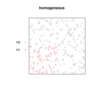
(a)

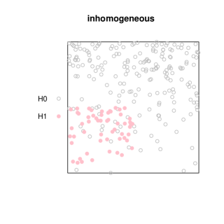
(b)

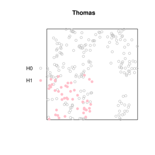
(c)

(d)

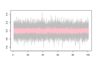
(e)

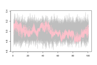
(f)

Figure 4: Simulation scenarios. Top panels: spatial ground patterns; Bottom panels: functional marks of model (11) (in grey) and of the marking models in item 1, 2, and 3, from left to right (in pink).

We show the results of the local test in terms of true-positive rate (TPR), false-positive rate (FPR), and accuracy (ACC), averaging over 100 simulated point patterns in Table 1. The rates are defined as

$$TPR=\frac{\text{true positives}}{\text{positives}},\quad FPR=\frac{\text{false negatives}}{\text{negatives}},\quad ACC=\frac{\text{true positives and negatives}}{\text{positives and negatives}}.$$

We of course wish to have TPR and ACC close to 1 and FPR close to 0.

As shown in Table 1, the performance of the local test in terms of classification rates strongly depends on the difference in the functional marks. Specifically, changing only the mean of the underlying random field is not enough for properly identifying the points of the feature patterns. This sufficiently improves when changing the variance only, but the best result is obtained when the whole model is changed, that is, changing the correlation structure. The effect of the type of ground pattern is less evident but still present. The inhomogeneous Poisson scenario reports the best classification rates, followed by the Thomas and homogeneous Poisson ones.

Finally, we found that the test function $t(\cdot)$ based on the $L_{2}$ distance in Equation (9) gave the better results overall. To further explore how the choice of test function influences the test, we also compared to a test function incorporating a derivative function accounting for the shape of the functional marks. This yielded similar results but turned out to be more computationally demanding.

Table 1: Results of the local test averaged over 100 simulated point patterns with an expected point count of 250 each.

Ground process	Marking model	TPR	FPR	ACC
Homogeneous Poisson	(1)	0.112	0.346	0.583
Homogeneous Poisson	(2)	0.583	0.066	0.820
Homogeneous Poisson	(3)	0.870	0.024	0.896
Inhomogeneous Poisson	(1)	0.032	0.585	0.449
Inhomogeneous Poisson	(2)	0.648	0.084	0.856
Inhomogeneous Poisson	(3)	0.895	0.023	0.932
Thomas	(1)	0.109	0.394	0.571
Thomas	(2)	0.637	0.088	0.846
Thomas	(3)	0.865	0.025	0.925

7 Real seismic data analysis

We analyse data coming from the ISTANCE dataset, presented in Section 2. More specifically, we analyse a sample dataset provided at http://www.pi.ingv.it/instance/. The dataset contains 10000 records of 300 events, together with the associated metadata. Figure 5 shows the earthquake locations and time occurrences.

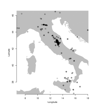
Figure 5: Earthquake locations and time occurrences

We first compute the proposed local $K$-function. The left panels of Figure 6 depict the estimated local summary statistics. In particular, the green lines represent the global statistics, while the grey ones represent the individual contributions. In blue we also represent the theoretical value. In the top-left panel, the $K$-function is based on a kernel intensity estimate whose bandwidth is selected by Diggle, (2013)’s rule, while in the bottom-left panel the bandwidth is chosen as in Cronie and Van Lieshout, (2018). We observe some relevant differences: while with Diggle, (2013)’s rule we depict different local $K$-functions deviating from the global one, following Cronie and Van Lieshout, (2018), we find a unique outlying local $K$-function. This may be explained by the fact that Cronie and Van Lieshout, (2018)’s approach tends to yield a bit too large bandwidths when large parts of the study region contain no points, while Diggle, (2013)’s approach tends to yield too small bandwidths in general; see Cronie and Van Lieshout, (2018) for details. Note that by increasing the bandwidth we decrease the intensity estimate and, as a consequence, the summand denominators in (8) are decreased. Therefore, we run the proposed local test of random labelling with both options for the bandwidth selection and, as expected, the differences observed in the computation of the local $K$-functions are reflected in the results of the test.

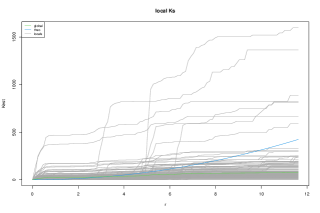
(a)

(b)

(c)

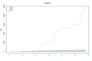
(d)

(e)

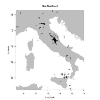
(f)

Figure 6: Left panels: Local $K$-functions. Center and right panels: Results of the local test at $\alpha=0.1$. Top panels: The $K$-function is based on a kernel intensity estimate whose bandwidth is selected by Diggle, (2013)’s rule. Bottom panels: The bandwidth is chosen as in Cronie and Van Lieshout, (2018).

Figure 6 displays the significant points (center panels) and the non-significant ones (right panels). The top panels show the results with Diggle, (2013)’s bandwidth while the bottom ones are obtained with Cronie and Van Lieshout, (2018)’s bandwidth. For both choices, we selected a significance level of $0.1$. We observe that the significant points tend to be similar in both cases, therefore the choice of bandwidth (selection method) does not seem to be crucial. We note that such bandwidth-induced differences were missing in the previously run simulation study. We attribute this sensitivity of the procedure to the shapes of the functional marks, that are obviously more variable, if compared to the simulated ones.

Nevertheless, both bandwidths lead to significant events belonging to important well known Italian seismic sequences. Of course these sequences are likely generated by different underlying processes, giving rise to long-term and highly correlated aftershocks.

8 Conclusions

In this work, we have proposed a general form for local summary statistics for marked point processes, which has been exploited to define the family of local inhomogeneous mark-weighted summary statistics for spatial point processes with functional marks, i.e. Functional Marked Point Processes (FMPP). We have employed such local summary statistics to construct a local test for random labelling, that is, to identify points, as well as regions, where this hypothesis does not hold.

More specifically, we first introduce a general local function for marked point patterns. With this specification, we are able to show that this function may be exploited to generate most summary statistics established in the literature. With particular reference to the functional marked context, we define the family of local $t$-weighted marked $n$-th order inhomogeneous summary statistics based on the $K$-function, which is a local contribution to a global summary statistic estimator. We obtain a result for the expectation of the general local summary statistic and exploit it to derive an expression for the expectation of our $t$-weighted local statistics.

Having access to these tools, we have proposed a local test of random labelling, resorting to the second order version of our proposed local estimator, obtaining a local test useful for identifying specific regions where a global test would not detect atypical behaviour of the points.

To study the performance of the test in terms of classification rates, we have conducted a simulation study, considering a number of scenarios with different ground processes and structures for the functional marks. Such simulations have shown that in many settings, the local test performs well in identifying points of a pattern where the hypothesis of random labelling is not verified.

We can draw a number of future work paths. Nevertheless, the local functions proposed in this paper can be considered as a very informative synthesis of the local second order behavior, useful for characterising the study area by an extended marked model, based on the FMPP theory. Incorporating local characteristics as functional marks would become part of the so called Constructed functional marks (CFMs), which are marks reflecting the geometries of point configurations in neighbourhoods of the individual points.

Concerning the application to seismic data, we aim at including also auxiliary (non-functional) marks into the analysis. These could contain synthetic information about the waveforms, such as the arrival times of the seismic event, or the inter-time between the two. The achievement of the unification of earthquake data and the FMPP theory would result in building a framework where it would be possible to exploit the available information of the seismic point process altogether.

A final comment concerns the possible extension of this paper’s tools to spatio-temporal ground processes, which of course are of importance for processes which typically exhibit spatio-temporal interactions, such as the seismic one.

References

- Adelfio et al., (2011) Adelfio, G., Chiodi, M., D’Alessandro, A., and Luzio, D. (2011). Fpca algorithm for waveform clustering. Journal of Communication and Computer, 8(6):494–502.
- Adelfio et al., (2012) Adelfio, G., Chiodi, M., D’Alessandro, A., Luzio, D., D’Anna, G., and Mangano, G. (2012). Simultaneous seismic wave clustering and registration. Computers & geosciences, 44:60–69.
- Adelfio et al., (2020) Adelfio, G., Siino, M., Mateu, J., and Rodríguez-Cortés, F. J. (2020). Some properties of local weighted second-order statistics for spatio-temporal point processes. Stochastic Environmental Research and Risk Assessment, 34(1):149–168.
- Anselin, (1995) Anselin, L. (1995). Local indicators of spatial association-lisa. Geographical analysis, 27(2):93–115.
- Anselin, (1996) Anselin, L. (1996). Chapter eight the moran scatterplot as an esda tool to assess local instability in spatial association. Spatial Analytical, 4:121.
- Baddeley et al., (2000) Baddeley, A. J., Møller, J., and Waagepetersen, R. (2000). Non-and semi-parametric estimation of interaction in inhomogeneous point patterns. Statistica Neerlandica, 54(3):329–350.
- Chiodi et al., (2013) Chiodi, M., Adelfio, G., D’Alessandro, A., and Luzio, D. (2013). Clustering and registration of multidimensional functional data. In Statistical Models for Data Analysis, pages 89–97. Springer.
- Chiu et al., (2013) Chiu, S. N., Stoyan, D., Kendall, W. S., and Mecke, J. (2013). Stochastic Geometry and Its Applications. John Wiley & Sons, third edition.
- Comas et al., (2011) Comas, C., Delicado, P., and Mateu, J. (2011). A second order approach to analyse spatial point patterns with functional marks. Test, 20(3):503–523.
- Cressie and Collins, (2001) Cressie, N. and Collins, L. B. (2001). Analysis of spatial point patterns using bundles of product density lisa functions. Journal of agricultural, biological, and environmental statistics, 6(1):118–135.
- Cronie and Van Lieshout, (2015) Cronie, O. and Van Lieshout, M. (2015). A J-function for inhomogeneous spatio-temporal point processes. Scandinavian Journal of Statistics, 42(2):562–579.
- Cronie and van Lieshout, (2016) Cronie, O. and van Lieshout, M. N. M. (2016). Summary statistics for inhomogeneous marked point processes. Annals of the Institute of Statistical Mathematics, 68(4):905–928.
- Cronie and Van Lieshout, (2018) Cronie, O. and Van Lieshout, M. N. M. (2018). A non-model-based approach to bandwidth selection for kernel estimators of spatial intensity functions. Biometrika, 105(2):455–462.
- Daley and Vere-Jones, (2008) Daley, D. J. and Vere-Jones, D. (2008). An Introduction to the Theory of Point Processes. Volume II: General Theory and Structure. Springer-Verlag, New York, second edition.
- D’Angelo et al., (2021) D’Angelo, N., Adelfio, G., and Mateu, J. (2021). Assessing local differences between the spatio-temporal second-order structure of two point patterns occurring on the same linear network. Spatial Statistics, 45:100534.
- (16) D’Angelo, N., Adelfio, G., and Mateu, J. (2022a). Locally weighted minimum contrast estimation for spatio-temporal log-gaussian cox processes. Submitted.
- (17) D’Angelo, N., Siino, M., D’Alessandro, A., and Adelfio, G. (2022b). Local spatial log-gaussian cox processes for seismic data. Advances in Statistical Analysis. https://doi.org/10.1007/s10182-022-00444-w.
- Diggle, (1985) Diggle, P. (1985). A kernel method for smoothing point process data. Journal of the Royal Statistical Society: Series C (Applied Statistics), 34(2):138–147.
- Diggle, (2013) Diggle, P. J. (2013). Statistical Analysis of Spatial and Spatio-Temporal Point Patterns. CRC Press.
- Gabriel and Diggle, (2009) Gabriel, E. and Diggle, P. J. (2009). Second-order analysis of inhomogeneous spatio-temporal point process data. Statistica Neerlandica, 63(1):43–51.
- Gelfand et al., (2010) Gelfand, A. E., Diggle, P., Guttorp, P., and Fuentes, M. (2010). Handbook of spatial statistics. CRC press.
- Getis and Franklin, (1987) Getis, A. and Franklin, J. (1987). Second-order neighborhood analysis of mapped point patterns. Ecology, 68(3):473–477.
- Getis and Ord, (1992) Getis, A. and Ord, J. K. (1992). The analysis of spatial association by use of distance statistics. Geographical Analysis, 24(3):189–206.
- Ghorbani et al., (2021) Ghorbani, M., Cronie, O., Mateu, J., and Yu, J. (2021). Functional marked point processes: a natural structure to unify spatio-temporal frameworks and to analyse dependent functional data. Test, 30(3):529–568.
- Iftimi et al., (2019) Iftimi, A., Cronie, O., and Montes, F. (2019). Second-order analysis of marked inhomogeneous spatiotemporal point processes: Applications to earthquake data. Scandinavian Journal of Statistics, 46(3):661–685.
- Illian et al., (2006) Illian, J., Benson, E., Crawford, J., and Staines, H. (2006). Principal component analysis for spatial point processes—assessing the appropriateness of the approach in an ecological context. In Case studies in spatial point process modeling, pages 135–150. Springer.
- Illian et al., (2008) Illian, J., Penttinen, A., Stoyan, H., and Stoyan, D. (2008). Statistical Analysis and Modelling of Spatial Point Patterns, volume 70. John Wiley & Sons.
- Mateu et al., (2007) Mateu, J., Lorenzo, G., and Porcu, E. (2007). Detecting features in spatial point processes with clutter via local indicators of spatial association. Journal of Computational and Graphical Statistics, 16(4):968–990.
- Mateu et al., (2010) Mateu, J., Lorenzo, G., and Porcu, E. (2010). Features detection in spatial point processes via multivariate techniques. Environmetrics, 21(3-4):400–414.
- Michelini et al., (2021) Michelini, A., Cianetti, S., Gaviano, S., Giunchi, C., Jozinović, D., and Lauciani, V. (2021). Instance–the italian seismic dataset for machine learning. Earth System Science Data, 13(12):5509–5544.
- Møller, (2003) Møller, J. (2003). Shot noise cox processes. Advances in Applied Probability, pages 614–640.
- Møller and Ghorbani, (2012) Møller, J. and Ghorbani, M. (2012). Aspects of second-order analysis of structured inhomogeneous spatio-temporal point processes. Statistica Neerlandica, 66(4):472–491.
- Møller and Waagepetersen, (2003) Møller, J. and Waagepetersen, R. P. (2003). Statistical Inference and Simulation for Spatial Point Processes. Chapman and Hall/CRC, Boca Raton.
- Moraga and Montes, (2011) Moraga, P. and Montes, F. (2011). Detection of spatial disease clusters with lisa functions. Statistics in Medicine, 30(10):1057–1071.
- Mrkvička et al., (2021) Mrkvička, T., Dvořák, J., González, J. A., and Mateu, J. (2021). Revisiting the random shift approach for testing in spatial statistics. Spatial Statistics, 42:100430.
- Myllymäki et al., (2017) Myllymäki, M., Mrkvička, T., Grabarnik, P., Seijo, H., and Hahn, U. (2017). Global envelope tests for spatial processes. Journal of the Royal Statistical Society: Series B (Statistical Methodology), 79(2):381–404.
- Penttinen and Stoyan, (1989) Penttinen, A. and Stoyan, D. (1989). Statistical analysis for a class of line segment processes. Scandinavian Journal of Statistics, pages 153–168.
- R Core Team, (2022) R Core Team (2022). R: A Language and Environment for Statistical Computing. R Foundation for Statistical Computing, Vienna, Austria.
- Ramsay and Silverman, (2002) Ramsay, J. O. and Silverman, B. W. (2002). Applied functional data analysis: methods and case studies, volume 77. Springer.
- Ripley, (1976) Ripley, B. D. (1976). The second-order analysis of stationary point processes. Journal of Applied Probability, 13:255–266.
- Schlather, (2001) Schlather, M. (2001). On the second-order characteristics of marked point processes. Bernoulli, pages 99–117.
- Siino et al., (2017) Siino, M., Adelfio, G., Mateu, J., Chiodi, M., and D’alessandro, A. (2017). Spatial pattern analysis using hybrid models: an application to the hellenic seismicity. Stochastic Environmental Research and Risk Assessment, 31(7):1633–1648.
- Siino et al., (2018) Siino, M., Rodríguez-Cortés, F. J., Mateu, J., and Adelfio, G. (2018). Testing for local structure in spatiotemporal point pattern data. Environmetrics, 29(5-6):e2463.
- Stoyan and Stoyan, (1994) Stoyan, D. and Stoyan, H. (1994). Fractals, Random Shapes and Point Fields: methods of geometrical statistics. Wiley, Chichester.
- Van Lieshout, (2000) Van Lieshout, M. (2000). Markov point processes and their applications. World Scientific.
- Van Lieshout, (2006) Van Lieshout, M. (2006). A j-function for marked point patterns. Annals of the Institute of Statistical Mathematics, 58(2):235–259.
- Van Rossum and Drake Jr, (1995) Van Rossum, G. and Drake Jr, F. L. (1995). Python reference manual. Centrum voor Wiskunde en Informatica Amsterdam.