Doubly-polarized $WZ$ hadronic production at NLO QCD+EW: Calculation method and further results

Abstract

The doubly-polarized production of $W^{\pm}Z$ pairs at the Large Hadron Collider (LHC) is presented at next-to-leading order (NLO) accuracy both for the electroweak (EW) and QCD corrections, including a detailed description of the calculational method using the double-pole approximation. Numerical results at the 13 TeV LHC are presented in particular for the $W^{-}Z$ case in the $e^{-}\bar{\nu}_{e}\mu^{+}\mu^{-}$ channel using ATLAS fiducial cuts and for polarized distributions defined in the $WZ$ center-of-mass system. The NLO EW corrections relative to the NLO QCD predictions are found to be smaller than $5\%$ in most kinematic distributions, but can reach the level of $10\%$ in some distributions such as lepton transverse momentum distributions or rapidity separation between the electron and the $Z$ boson. EW corrections are not uniform for different polarizations. A comparison between the new ATLAS measurement of polarization fractions to our theoretical prediction is presented.

1 Introduction

The Standard Model (SM) of particle physics is the current framework which describes how matter is organized at the most fundamental level. It allows for a consistent description of the interactions between quarks and leptons via the exchange of gauge bosons, in particular the $W$ and $Z$ bosons that are mediators of the electroweak (EW) interaction. The CERN Large Hadron Collider (LHC) has produced lots of such EW gauge bosons since the beginning of its operation, and the amount of collected data in both run I and run II has allowed for a detailed study of the properties of the $W$ and the $Z$ bosons. It is expected that with run III starting in 2022, theorists and experimentalists will be able to search for more potential new-physics effects in the tail of gauge boson differential distributions, as well as access to a precise determination of polarization observables of the $W$ and $Z$ bosons. The four-lepton channel via $ZZ$ production and the three-lepton channel via $WZ$ productions are of prime importance for such polarization studies, see for example the latest ATLAS ATLAS:2021wob and CMS results CMS:2021icx in the three-lepton channel, using the full run II dataset, as well as ATLAS differential results in the four-lepton channel ATLAS:2021kog .

In order to allow for a meaningful comparison with experiments, the theory prediction has to reach a high accuracy and higher order QCD and EW corrections are needed. The next-to-leading order (NLO) QCD corrections in the $WZ$ channel were calculated in Refs. Ohnemus:1991gb ; Frixione:1992pj for on-shell production and in Refs. Dixon:1998py ; Dixon:1999di for off-shell production including the leptonic decays. The NLO EW corrections were calculated in Refs. Accomando:2004de ; Bierweiler:2013dja ; Baglio:2013toa ; Biedermann:2017oae , demonstrating the importance of the quark-photon real corrections in an inclusive setup. The next-to-next-to-leading order (NNLO) QCD corrections were obtained for the first time in 2015 Gehrmann:2015ora ; Grazzini:2016swo ; Grazzini:2017ckn while the combination of NNLO QCD corrections with NLO EW corrections was performed in 2019 Grazzini:2019jkl . The comparison of theory predictions with experimental observables also requires soft gluon effects to be taken into account. This was performed in Refs. Melia:2011tj ; Nason:2013ydw at NLO QCD in parton shower programs and then later extended to a consistent matching of NLO QCD+EW corrections to parton shower in Ref. Chiesa:2020ttl . In order to study new physics effects, the effect of SM effective theory operators was included at NLO QCD+EW via anomalous couplings in Ref. Chiesa:2018lcs and taken into account in parton shower programs at NLO QCD in Refs. Baglio:2019uty ; Baglio:2020oqu . Full NLO QCD predictions including full off-shell and spin-correlation effects for leptonic final states can now be easily obtained with the help of computer tools such as MCFM Campbell:1999ah ; Campbell:2011bn or VBFNLO Arnold:2008rz ; Baglio:2014uba .

All this progress in the calculation of higher-order corrections has also helped to increase the accuracy of the theoretical predictions for angular observables and polarized cross sections. Thanks to the wealth of data at the LHC it is now possible to also get experimental results for polarization observables in the three- and four-lepton channels. Even the two-lepton channel has been given some attention, see the NNLO QCD theory perspective in Ref. Poncelet:2021jmj . As the two-lepton channel is more difficult to measure because of the amount of missing energy, this paper will focus on the three-lepton channel using $WZ$ production.

Experimental results for singly-polarized observables in the three-lepton channel were first presented by ATLAS in 2019 ATLAS:2019bsc using run II data at 13 TeV. They have been updated very recently including a measurement, for the first time, of the double polarization of $WZ$ events, in particular involving longitudinally polarized gauge bosons ATLAS:2022conf53 . The LO prediction for polarized cross sections were presented in the 80s Bilchak:1984gv ; Willenbrock:1987xz while the NLO QCD corrections were studied much later Stirling:2012zt . The NLO EW corrections to gauge boson polarization observables in the $WZ$ channel were first calculated in Refs. Baglio:2018rcu ; Baglio:2019nmc and combined with QCD corrections. The idea of this study is to define polarization observables, which we termed fiducial polarizations, directly from lepton angular distributions. The same idea has been implemented in Refs. Rahaman:2018ujg ; Rahaman:2019lab , using polarization asymmetries to constrain anomalous triple gauge boson couplings. The advantage of this approach is that the observables can be easily calculated at any order in perturbation theory with arbitrary kinematic cuts on the leptons using available calculations for unpolarized cross sections. This has been shown to work for single polarizations. Whether similar observables can be defined for double polarization is still an open question. The negative side of this method is that the values of those observables depend strongly on the lepton cuts, hence can be very different from the values obtained using the on-shell gauge boson approximation.

The traditional method to define gauge boson polarization is using the on-shell approximation, allowing for a separation of the gauge-boson polarizations at the amplitude level. Following this path, doubly-polarized predictions for the two-lepton channel ($W^{+}W^{-}$) Denner:2020bcz , three-lepton channel ($W^{\pm}Z$) Denner:2020eck , and four-lepton channel ($ZZ$) Denner:2021csi were obtained at NLO in QCD in 2020 and 2021 using the double-pole approximation (DPA). The calculation in the $ZZ$ channel includes EW corrections as well, see Ref. Denner:2021csi . It is worth noticing that, because this polarization separation is done at the amplitude level (in contrast to the above fiducial polarizations which are defined at the cross section level), it requires a careful definition of the on-shell momenta and other technical details. The nice thing of this approach is that it allows for generation of fully polarized events.

Inspired by these results, we have extended their method to cover the three-lepton channel ($W^{\pm}Z$), where a new ingredient must be added to deal with the photon radiation off the intermediate on-shell $W$ boson. In Le:2022lrp we have already presented our first results at the NLO QCD+EW level for the $W^{+}Z$ production using the same fiducial cuts and reference frame as ATLAS ATLAS:2019bsc . The goal of the paper is to present the complete description of the calculation method behind the results of Ref. Le:2022lrp , as well as give results for the $W^{-}Z$ channel. We will also perform a comparison between our NLO QCD+EW predictions and the new ATLAS measurement ATLAS:2022conf53 for the doubly-polarized cross sections.

The paper is organized as follows. The definition of polarizations is given in Section 2. The details of the calculation of the QCD corrections are briefly given in Section 3 while the EW corrections are explained in depth in Section 4, first with the description of the method to calculate the EW corrections to the production part in Subsection 4.1, and then to the decay part in Subsection 4.2. The numerical results using the ATLAS fiducial cuts and the $WZ$ center-of-mass system (c.m.s) reference frame at the LHC at 13 TeV, mainly for the $W^{-}Z$ channel, are presented in Section 5. This section starts with the integrated polarized cross sections that are given in Subsection 5.1, where the comparison with the ATLAS measurement is provided. The relevant kinematical distributions are then shown in Subsection 5.2. We conclude in Section 6.

2 Definition of polarizations

We study the polarized production of three charged leptons plus missing energy at hadron colliders, so that the process of interest is

$$p(k_{1})+p(k_{2})\to\ell_{1}(k_{3})+\ell_{2}(k_{4})+\ell_{3}(k_{5})+\ell_{4}(k_{6})+X,$$ (1)

where the final-state leptons can be either $e^{+}\nu_{e}\mu^{+}\mu^{-}$ or $e^{-}\bar{\nu}_{e}\mu^{+}\mu^{-}$. Representative Feynman diagrams at leading order (LO) are depicted in Fig. 1. They can be divided in two categories: either the upper row of Fig. 1 where the intermediate $W$ and $Z$ bosons (or photon) both split into final-state leptons, or the lower row of Fig. 1 which contains only singly-resonant diagrams with $W\to 4\ell$ splitting. We are interested in the kinematical region where the final-state leptons originate from nearly on-shell (OS) gauge bosons, so that the process in Eq. (1) can be seen as

$$p(k_{1})+p(k_{2})\to V_{1}(q_{1})+V_{2}(q_{2})\to\ell_{1}(k_{3})+\ell_{2}(k_{4})+\ell_{3}(k_{5})+\ell_{4}(k_{6})+X,$$ (2)

where the intermediate gauge bosons are $V_{1}=W^{\pm}$, $V_{2}=Z$. In practice this means we are neglecting the diagrams depicted in the lower row of Fig. 1 as well as the photon contribution of the upper row of Fig. 1. In this way we will be able to define polarized cross sections and get a clear separation of the polarizations of the intermediate gauge bosons. This is called the double-pole approximation (DPA), where contributions from $W\to 4\ell$ and very off-shell $WZ$ contributions are neglected because they are strongly suppressed by the kinematical cuts. In the DPA, the whole process can be viewed as an OS production of $WZ$ followed by the OS decays $W^{\pm}\to e^{\pm}\nu_{e}$ and $Z\to\mu^{+}\mu^{-}$, connected via off-shell $W$ and $Z$ propagators and keeping the spin correlations.

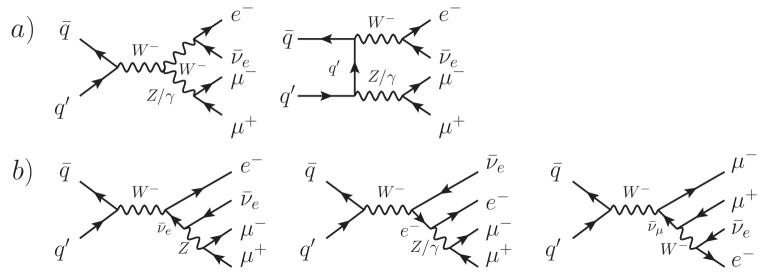
Figure 1: Double and single resonant diagrams at leading order. Group a) includes both double and single resonant diagrams, while group b) is only single resonant.

The (unpolarized) amplitude for the process in Eq. (1) is defined at LO in the DPA as (see also Ref. Denner:2000bj for $e^{+}e^{-}\to W^{+}W^{-}\to 4$ fermions)

$$\mathcal{A}_{\text{LO,DPA}}^{\bar{q}q^{\prime}\to V_{1}V_{2}\to 4l}=\frac{1}{Q_{1}Q_{2}}\sum_{\lambda_{1},\lambda_{2}=1}^{3}\mathcal{A}_{\text{LO}}^{\bar{q}q^{\prime}\to V_{1}V_{2}}(\hat{k}_{i})\mathcal{A}_{\text{LO}}^{V_{1}\to\ell_{1}\ell_{2}}(\hat{k}_{i})\mathcal{A}_{\text{LO}}^{V_{2}\to\ell_{3}\ell_{4}}(\hat{k}_{i}),$$ (3)

with

$$Q_{j}=q_{j}^{2}-M_{V_{j}}^{2}+iM_{V_{j}}\Gamma_{V_{j}}\,(j=1,2),$$ (4)

where $q_{1}=k_{3}+k_{4}$, $q_{2}=k_{5}+k_{6}$, $M_{V}$ and $\Gamma_{V}$ are the physical mass and width of the gauge bosons, and $\lambda_{j}$ are the polarization indices of the gauge bosons. A similar factorization in the terms of the sum holds at higher orders in perturbation theory. It is crucial that all helicity amplitudes $\mathcal{A}$ in the numerator are calculated using OS momenta $\hat{k}_{i}$ for the final-state leptons as well as OS momenta $\hat{q}_{j}$ for the intermediate gauge bosons, derived from the off-shell (full process) momenta $k_{i}$ and $q_{j}$, in order to ensure that gauge invariance in the amplitudes is preserved. An OS mapping is used to obtain the OS momenta $\hat{k}_{i}$ from the off-shell momenta $k_{i}$. This OS mapping is not unique, however it is known that the induced shift by different mappings is of order $\alpha\Gamma_{V}/(\pi M_{V})$ Denner:2000bj . The next sections will provide the explicit details on the mappings used in our calculation.

The sum over the polarization index $\lambda_{j}$ for a given gauge boson runs from 1 to 3, because a massive gauge boson has three physical polarization states: two transverse states $\lambda=1$ and $\lambda=3$ (left and right) and one longitudinal state $\lambda=2$. In total the diboson system has then 9 polarization states, each of them can be singled out of Eq. (3) by selecting only the desired $\lambda_{j}$ in the sum. We will define four main doubly-polarized cross sections in this paper:

• The longitudinal-longitudinal (LL, or $W^{\pm}_{L}Z_{L}$) contribution, obtained with selecting only $\lambda_{1}=\lambda_{2}=2$ in the sum of Eq. (3);

• The transverse-transverse (TT, or $W^{\pm}_{T}Z_{T}$) contribution, obtained with selecting only $\lambda_{1}\neq 2$ and $\lambda_{2}\neq 2$ in the sum of Eq. (3), taking into account the interference between the various individual transverse polarization states of the two gauge boson;

• The longitudinal-transverse (LT, or $W^{\pm}_{L}Z_{T}$) contribution, obtained with selecting only $(\lambda_{1},\lambda_{2})=(2,1)+(2,3)$;

• The transverse-longitudinal (TL, or $W^{\pm}_{T}Z_{L}$) contribution, obtained with selecting only $(\lambda_{1},\lambda_{2})=(1,2)+(3,2)$.

In addition we will call “interference” the difference between the unpolarized contribution (where all polarization amplitudes are summed before squaring) and the sum of the LL, TT, LT, and TL cross sections.

We will present in the next sections our detailed calculation of the NLO QCD and EW corrections in the DPA and focus on those doubly-polarized contributions that we have defined above. While the unpolarized cross section is Lorentz invariant because all possible helicity states are summed over, the doubly-polarized cross sections depend on the reference frame. As done in Ref. Le:2022lrp we will provide results in the $WZ$ center-of-mass system, following ATLAS choice in Ref. ATLAS:2019bsc . The same set of kinematic cuts will be used. Note that the NLO QCD corrections have already been presented in Ref. Denner:2020eck where the computation method is identical to the one used for the $WW$ channel Denner:2000bj and for the $ZZ$ production Denner:2021csi . We follow the same steps and re-describe here the NLO QCD calculation method to prepare the framework and notations for the NLO EW calculation.

3 NLO QCD

The master formulas for the virtual, real-gluon emission, and quark-gluon induced amplitudes are schematically written as follows,

$$\delta\mathcal{A}_{\text{virt,QCD}}^{\bar{q}q^{\prime}\to V_{1}V_{2}\to 4l} =\frac{1}{Q_{1}Q_{2}}\sum_{\lambda_{1},\lambda_{2}}\delta\mathcal{A}_{\text{virt,QCD}}^{\bar{q}q^{\prime}\to V_{1}V_{2}}(\hat{k})\mathcal{A}_{\text{LO}}^{V_{1}\to\ell_{1}\ell_{2}}(\hat{k})\mathcal{A}_{\text{LO}}^{V_{2}\to\ell_{3}\ell_{4}}(\hat{k}),$$ (5)

$$\delta\mathcal{A}_{\text{g-rad}}^{\bar{q}q^{\prime}\to V_{1}V_{2}g\to 4lg} =\frac{1}{Q_{1}Q_{2}}\sum_{\lambda_{1},\lambda_{2}}\delta\mathcal{A}_{\text{g-rad}}^{\bar{q}q^{\prime}\to V_{1}V_{2}g}(\hat{k})\mathcal{A}_{\text{LO}}^{V_{1}\to\ell_{1}\ell_{2}}(\hat{k})\mathcal{A}_{\text{LO}}^{V_{2}\to\ell_{3}\ell_{4}}(\hat{k}),$$ (6)

$$\delta\mathcal{A}_{\text{g-ind}}^{qg\to V_{1}V_{2}q^{\prime}\to 4lq^{\prime}} =\frac{1}{Q_{1}Q_{2}}\sum_{\lambda_{1},\lambda_{2}}\delta\mathcal{A}_{\text{g-ind}}^{qg\to V_{1}V_{2}q^{\prime}}(\hat{k})\mathcal{A}_{\text{LO}}^{V_{1}\to\ell_{1}\ell_{2}}(\hat{k})\mathcal{A}_{\text{LO}}^{V_{2}\to\ell_{3}\ell_{4}}(\hat{k}),$$ (7)

where the correction amplitudes $\delta\mathcal{A}_{\text{virt,QCD}}^{\bar{q}q^{\prime}\to V_{1}V_{2}}$, $\delta\mathcal{A}_{\text{g-rad}}^{\bar{q}q^{\prime}\to V_{1}V_{2}g}$, and $\delta\mathcal{A}_{\text{g-ind}}^{qg\to V_{1}V_{2}q^{\prime}}$ have been calculated in the OS production calculation in Ref. Baglio:2013toa and are reused here. The amplitudes are for the unpolarized process; for the polarized amplitudes the corresponding $\lambda_{i,j}$ have to be selected in the sum. Note that the amplitude factors on the r.h.s have to be calculated using suitable OS mapped momenta denoted by the hat. Details of the OS mappings are below provided. The propagator factors $Q_{i}$ are computed using the off-shell momenta.

For the real corrections Eq. (6) and Eq. (7), since the amplitudes are divergent in the IR limits we employ the dipole subtraction method Catani:1996vz ; Dittmaier:1999mb to calculate the NLO cross section. In this formalism, the full differential cross section is written as, using similar notation as in Ref. Denner:2021csi :

$$\left(\frac{d\sigma}{d\xi}\right)_{\text{NLO}}= \int d\Phi_{n}^{(4)}\mathcal{B}(\Phi_{n}^{(4)})\delta(\xi-\xi_{n})$$

$$+\int d\Phi_{n}^{(4)}\left[\mathcal{V}(\Phi_{n}^{(D)})+\mathcal{C}(\Phi_{n}^{(D)})+\int d\Phi_{\text{rad}}^{(D)}\mathcal{D}_{\text{int}}(\Phi_{n}^{(D)},\Phi_{\text{rad}}^{(D)})\right]_{D=4}\delta(\xi-\xi_{n})$$

$$+\int d\Phi_{n+1}^{(4)}\left[\mathcal{R}(\Phi_{n+1}^{(4)})\delta(\xi-\xi_{n+1})-\mathcal{D}_{\text{sub}}(\tilde{\Phi}_{n}^{(4)},\Phi_{\text{rad}}^{(4)})\delta(\xi-\tilde{\xi}_{n})\right],$$ (8)

where $\mathcal{B}$ and $\mathcal{V}$ are the Born and virtual contributions. The flux factor is included in the matrix elements. $\mathcal{R}$ is the real correction term, which includes the amplitudes $\delta\mathcal{A}_{\text{g-rad}}$ and $\delta\mathcal{A}_{\text{g-ind}}$ above defined. Note that $\xi$ is a placeholder for any differential variable that is of interest: the $p_{T}$ of one of the final-state leptons, the invariant masses, angle, etc. $\mathcal{D}_{\text{sub}}$ is the dipole subtraction term introduced in the Catani-Seymour (CS) formalism Catani:1996vz . For the NLO QCD, $\mathcal{D}_{\text{sub}}$ includes only the case of initial-state emitter and initial-state spectator. The corresponding integrated $\mathcal{D}_{\text{int}}$ term is placed in the same group with the virtual contribution and also depends on the radiation phase-space $\Phi_{\text{rad}}^{(D)}$ (here in $D$ dimensions). Finally, to cancel the left-over initial state collinear divergences, the collinear counter term $\mathcal{C}$ has to be added. The tilde placed on top of $\Phi_{n}$ and $\xi_{n}$ is to indicate that the momenta are calculated using the CS mappings. To regulate the IR divergences we use as default the mass regularization, i.e. introducing small mass parameters for the gluon and the light quarks (all but the top quark). We have verified that the result is in good agreement with the one obtained using dimensional regularization.

For the $\mathcal{R}$ contribution, we first generate a set of $(n+1)$ off-shell momenta $[k_{n+1}]$ in the partonic c.m.s. We then perform the following OS mapping:

• Boost all momenta to the $VV$ c.m.s;

• Perform the OS projection on the four lepton momenta. We call this OSVV4 mapping (which is the $\text{DPA}^{(2,2)}$ mapping in Denner:2021csi ),

  $$[\hat{k}_{n+1}]=\text{OSVV4 mapping}([k_{n+1}]),$$ (9)

  where VV indicates that this mapping has to be done in the $VV$ c.m.s and 4 to denote the $VV\to 4\,l$ transition (in the next section we will have $VV\to 4\,l+\gamma$ for NLO EW final-state radiation). We note that the $VV$ c.m.s of the new OS momenta $[\hat{k}_{n+1}]$ coincides with the $VV$ c.m.s of the off-shell momenta, because momentum conservation requires that

  $$\hat{q}_{1}+\hat{q}_{2}=q_{1}+q_{2},$$ (10)

  where $q_{1,2}$ are the momenta of the gauge bosons.

To be more explicit, the OSVV4 mapping is done as follows Denner:2021csi . After boosting all momenta to the VV c.m.s, we first calculate the OS momenta $\hat{q}_{i}$ which satisfy Eq. (10) together with the on-shellness $\hat{q}^{2}_{i}=M^{2}_{V_{i}}$. These conditions are however not enough to fix all the components of $\hat{q}_{i}$. For this, we choose that the spatial direction of the gauge bosons in the VV c.m.s is preserved as in Denner:2000bj , namely $\vec{\hat{q}}_{1}=b\vec{q}_{1}$ with $b$ being a real number. This coefficient $b$ is then easily calculated and the result is provided in Baglio:2018rcu (see Appendix A). The OS final-state lepton momenta are computed as Denner:2021csi :

• Boost $k_{e}$ and $k_{\nu_{e}}$ into the off-shell $W$ boson rest frame, calculate the spatial direction $\vec{n}_{e}$ in this frame;

• Set the spatial direction of $\hat{k}_{e}^{\prime}$ in the on-shell $W$ boson rest frame to be the same as in the off-shell $W$ boson rest frame, so that, in the on-shell $W$ boson rest frame, we have $\vec{\hat{k}}_{e}^{\prime}=\vec{n}_{e}\hat{k}_{e}^{\prime 0}$ with $\hat{k}_{e}^{\prime 0}=M_{W}/2$. For the neutrino $\vec{\hat{k}}_{\nu_{e}}^{\prime}=-\vec{\hat{k}}_{e}^{\prime}$ and $\hat{k}_{\nu_{e}}^{\prime 0}=\hat{k}_{e}^{\prime 0}$;

• Boost back the momenta $\hat{k}_{l}^{\prime}$ from the on-shell $W$ rest frame to the VV c.m.s using the boot parameters $\hat{q}_{1}$ to obtain the OS momenta $\hat{k}_{e}$ and $\hat{k}_{\nu_{e}}$.

The same procedure is applied to the $Z$ decay products, replacing above the $W$ boson by the $Z$ boson ($q_{1}$ by $q_{2}$, $k_{e}$ and $k_{\nu_{e}}$ by $k_{\mu^{+}}$ and $k_{\mu^{-}}$). The initial quark momenta are unchanged in this mapping.

For the subtraction term $\mathcal{D}_{\text{sub}}$, we first calculate the CS momenta (also called the CS reduced momenta) $[\tilde{k}_{n}]$ from the off-shell momenta $[k_{n+1}]$ (generated in the partonic c.m.s) using the CS mapping for the case of initial-state emitter and initial-state spectator as in Ref. Dittmaier:1999mb (massless case):

$$[\tilde{k}_{n}]=\text{CS mapping}([k_{n+1}]).$$ (11)

We then boost $[\tilde{k}_{n}]$ to the $VV$ c.m.s and perform the OSVV4 mapping to obtain a set of OS momenta:

$$[\hat{\tilde{k}}_{n}]=\text{OSVV4 mapping}([\tilde{k}_{n}]).$$ (12)

The DPA amplitudes for the subtraction terms are calculated similarly to Eq. (3) with the OS momenta $[\hat{\tilde{k}}_{n}]$ entering the amplitudes in the numerator and the off-shell momenta $[\tilde{k}_{n}]$ in the denominator factors $Q_{j}$. We note that $Q_{j}$ are Lorentz invariant hence it does not matter in which frame they are calculated. However, the helicity amplitudes in the numerator are not Lorentz invariant, hence they have to be calculated in the correct frame, which is the VV c.m.s in our case.

For kinematic cuts and distributions, we use the off-shell momenta $[k_{n+1}]$ for the $\mathcal{R}$ term and the CS mapped momenta $[\tilde{k}_{n}]$ for the $\mathcal{D}_{\text{sub}}$ term. These momenta have to be boosted from the partonic c.m.s to the Lab frame before applying cut constraints or filling histograms.

Concerning the integrated dipole terms, they are calculated as in Dittmaier:1999mb with the only addition that the OS mapping step has to be implemented when calculating the Born amplitudes. Since the same on-shell mapping is used in the $\mathcal{D}_{\text{sub}}$ term and in its integrated counterpart $\mathcal{D}_{\text{int}}$, the needed correspondence between these two terms are guaranteed.

4 NLO EW

NLO EW corrections in the DPA are divided into production and decay parts. For the production part, full NLO EW corrections to the process $\bar{q}q^{\prime}\to WZ$ are calculated. For the decay part, full NLO EW corrections to the decays $W\to e\nu_{e}$ and $Z\to\mu^{+}\mu^{-}$ are included. These are called factorizable corrections. The non-factorizable contribution, including interferences between the initial-state radiation and the final-state radiation, as defined in Baglio:2018rcu , is very small Beenakker:1997bp ; Denner:1997ia ; Denner:1998rh and hence neglected.

For the production part, the NLO amplitudes read

$$\delta\mathcal{A}_{\text{virt,prod}}^{\bar{q}q^{\prime}\to V_{1}V_{2}\to 4l} =\frac{1}{Q_{1}Q_{2}}\sum_{\lambda_{1},\lambda_{2}}\delta\mathcal{A}_{\text{virt,prod}}^{\bar{q}q^{\prime}\to V_{1}V_{2}}\mathcal{A}_{\text{LO}}^{V_{1}\to\ell_{1}\ell_{2}}\mathcal{A}_{\text{LO}}^{V_{2}\to\ell_{3}\ell_{4}},$$ (13)

$$\delta\mathcal{A}_{\text{$\gamma$-rad,prod}}^{\bar{q}q^{\prime}\to V_{1}V_{2}\to 4l\gamma} =\frac{1}{Q_{1}Q_{2}}\sum_{\lambda_{1},\lambda_{2}}\delta\mathcal{A}_{\text{$\gamma$-rad,prod}}^{\bar{q}q^{\prime}\to V_{1}V_{2}\gamma}\mathcal{A}_{\text{LO}}^{V_{1}\to\ell_{1}\ell_{2}}\mathcal{A}_{\text{LO}}^{V_{2}\to\ell_{3}\ell_{4}},$$ (14)

$$\delta\mathcal{A}_{\text{$\gamma$-ind,prod}}^{q\gamma\to V_{1}V_{2}q^{\prime}\to 4lq^{\prime}} =\frac{1}{Q_{1}Q_{2}}\sum_{\lambda_{1},\lambda_{2}}\delta\mathcal{A}_{\text{$\gamma$-ind,prod}}^{q\gamma\to V_{1}V_{2}q^{\prime}}\mathcal{A}_{\text{LO}}^{V_{1}\to\ell_{1}\ell_{2}}\mathcal{A}_{\text{LO}}^{V_{2}\to\ell_{3}\ell_{4}},$$ (15)

where the correction amplitudes $\delta\mathcal{A}_{\text{virt,prod}}^{\bar{q}q^{\prime}\to V_{1}V_{2}}$, $\delta\mathcal{A}_{\text{$\gamma$-rad,prod}}^{\bar{q}q^{\prime}\to V_{1}V_{2}\gamma}$, and $\delta\mathcal{A}_{\text{$\gamma$-ind,prod}}^{q\gamma\to V_{1}V_{2}q^{\prime}}$ have been calculated in the OS production calculation in Ref. Baglio:2013toa and are reused here.

For the $W$ decay part, we have

$$\delta\mathcal{A}_{\text{virt,W}}^{\bar{q}q^{\prime}\to V_{1}V_{2}\to 4l} =\frac{1}{Q_{1}Q_{2}}\sum_{\lambda_{1},\lambda_{2}}\mathcal{A}_{\text{LO}}^{\bar{q}q^{\prime}\to V_{1}V_{2}}\delta\mathcal{A}_{\text{virt}}^{V_{1}\to\ell_{1}\ell_{2}}\mathcal{A}_{\text{LO}}^{V_{2}\to\ell_{3}\ell_{4}},$$ (16)

$$\delta\mathcal{A}_{\text{$\gamma$-rad,W}}^{\bar{q}q^{\prime}\to V_{1}V_{2}\to 4l\gamma} =\frac{1}{Q^{\prime}_{1}Q_{2}}\sum_{\lambda_{1},\lambda_{2}}\mathcal{A}_{\text{LO}}^{\bar{q}q^{\prime}\to V_{1}V_{2}}\delta\mathcal{A}_{\text{$\gamma$-rad}}^{V_{1}\to\ell_{1}\ell_{2}\gamma}\mathcal{A}_{\text{LO}}^{V_{2}\to\ell_{3}\ell_{4}},$$ (17)

and for the $Z$ decay:

$$\delta\mathcal{A}_{\text{virt,Z}}^{\bar{q}q^{\prime}\to V_{1}V_{2}\to 4l} =\frac{1}{Q_{1}Q_{2}}\sum_{\lambda_{1},\lambda_{2}}\mathcal{A}_{\text{LO}}^{\bar{q}q^{\prime}\to V_{1}V_{2}}\mathcal{A}_{\text{LO}}^{V_{1}\to\ell_{1}\ell_{2}}\delta\mathcal{A}_{\text{virt}}^{V_{2}\to\ell_{3}\ell_{4}},$$ (18)

$$\delta\mathcal{A}_{\text{$\gamma$-rad,Z}}^{\bar{q}q^{\prime}\to V_{1}V_{2}\to 4l\gamma} =\frac{1}{Q_{1}Q^{\prime}_{2}}\sum_{\lambda_{1},\lambda_{2}}\mathcal{A}_{\text{LO}}^{\bar{q}q^{\prime}\to V_{1}V_{2}}\mathcal{A}_{\text{LO}}^{V_{1}\to\ell_{1}\ell_{2}}\delta\mathcal{A}_{\text{$\gamma$-rad}}^{V_{2}\to\ell_{3}\ell_{4}\gamma},$$ (19)

where the NLO decay amplitudes are generated by FormCalc Hahn:1998yk ; Hahn:2000kx . The new variables $Q^{\prime}_{1}$ and $Q^{\prime}_{2}$ are defined as in Eq. (4) but with the gauge-boson momenta being reconstructed from the off-shell $1\to 3$ decays.

As in the case of NLO QCD, the amplitude factors on the r.h.s of Eqs. (13-19) are calculated using on-shell momenta, while the factors $Q_{i}$ and $Q^{\prime}_{i}$ are off-shell.

4.1 NLO EW corrections to the production part

The differential cross section for the production part is calculated using the same formalism as in Eq. (8). The main differences compared to the NLO QCD case come from the real corrections because the photon can now be radiated off the on-shell $W$ boson, leading to new types of dipole terms in the CS subtraction function.

We split the $\mathcal{R}$ term in Eq. (8) into two parts

$$\mathcal{R}^{\text{prod}}=\mathcal{R}_{\text{$\gamma$-ind}}^{\text{prod}}+\mathcal{R}_{\text{$\gamma$-rad}}^{\text{prod}},$$ (20)

corresponding to two subtraction terms $\mathcal{D}_{\text{$\gamma$-ind}}^{\text{prod,sub}}$ and $\mathcal{D}_{\text{$\gamma$-rad}}^{\text{prod,sub}}$, respectively.

For the $\mathcal{R}_{\text{$\gamma$-ind}}^{\text{prod}}$ and $\mathcal{R}_{\text{$\gamma$-rad}}^{\text{prod}}$ terms, the OS momenta $[\hat{k}_{n+1}]$ are calculated using the same method as in the NLO QCD case. Concerning the dipole subtraction term ($\mathcal{D}_{\text{sub}}$) of the $\gamma$-induced process, the same method as in the NLO QCD case is used, meaning that the OS mapping is applied on top of the CS reduced momenta. The integrated counterpart is therefore treated accordingly with the same OS mapping. We note that the $\gamma\to W^{+}W^{-}$ splitting is finite due to the $W$ mass hence there is no subtraction term for this splitting. The Born amplitude in the subtraction term is therefore proportional to the $\bar{q}q^{\prime}\to V_{1}V_{2}\to 4l$ amplitude as in the NLO QCD case.

For the dipole subtraction term ($\mathcal{D}_{\text{sub}}$) of the $\gamma$-radiated process, there are two contributions: both emitter and spectator are initial-state particles or one is in the initial state the other is the OS $W$ boson. The latter one is needed, even though the $W$ is an intermediate particle, because the OS amplitude $\delta\mathcal{A}_{\text{$\gamma$-rad,prod}}^{\bar{q}q^{\prime}\to V_{1}V_{2}\gamma}$ in Eq. (14) contains soft divergences due to the photon radiation off an OS $W$. The case of initial-state emitter and initial-state spectator is treated identically to the NLO QCD process.

For the case of $W$ emitter and initial quark spectator, which is the case of final-state emitter and initial-state spectator in Dittmaier:1999mb , the subtraction function for the OS production $\bar{q}q^{\prime}\to WZ\gamma$ reads Dittmaier:1999mb

$$\mathcal{\hat{D}}_{\text{sub}}^{Wq}(\hat{k}) \sim\hat{g}_{\text{sub}}(\hat{k}_{a},\hat{k}_{W},\hat{k}_{\gamma})\mathcal{\hat{B}}(\tilde{\hat{k}}_{q},\tilde{\hat{k}}_{V}),$$ (21)

$$\hat{g}_{\text{sub}} =\frac{1}{(\hat{k}_{W}\hat{k}_{\gamma})\hat{x}_{ia}}\left(\frac{2}{2-\hat{x}_{ia}-\hat{z}_{ia}}-1-\hat{z}_{ia}-\frac{M_{W}^{2}}{\hat{k}_{W}\hat{k}_{\gamma}}\right),$$ (22)

$$\hat{x}_{ia} =\frac{\hat{k}_{a}\hat{k}_{W}+\hat{k}_{a}\hat{k}_{\gamma}-\hat{k}_{W}\hat{k}_{\gamma}}{\hat{k}_{a}\hat{k}_{W}+\hat{k}_{a}\hat{k}_{\gamma}},\quad\hat{z}_{ia}=\frac{\hat{k}_{a}\hat{k}_{W}}{\hat{k}_{a}\hat{k}_{W}+\hat{k}_{a}\hat{k}_{\gamma}},$$ (23)

$$\tilde{\hat{k}}_{W} =\hat{k}_{W}+\hat{k}_{\gamma}-(1-\hat{x}_{ia})\hat{k}_{a},\;\;\tilde{\hat{k}}_{a}=\hat{x}_{ia}\hat{k}_{a},$$ (24)

where the subscript $a$ denotes the initial spectator, $i$ denotes the final emitter and the remaining momenta $[\tilde{\hat{k}}]$ are the same as the corresponding momenta $[\hat{k}]$. The OS Born amplitude is $\mathcal{\hat{B}}$. When including the leptonic decays in the DPA framework we have

$$\mathcal{D}_{\text{sub}}^{Wq}(k)\delta(\xi-\tilde{\xi}_{n})\sim\hat{g}_{\text{sub}}(\hat{k}_{a},\hat{k}_{W},\hat{k}_{\gamma})\mathcal{B}(\hat{\tilde{k}}_{n},\tilde{Q}_{i})\delta(\xi-\tilde{\xi}_{n}),$$ (25)

where the OS momenta $[\hat{k}_{n+1}]$ are calculated from the off-shell $[k_{n+1}]$ as follows.

• Boost all lepton momenta from the partonic c.m.s to the $VV$ c.m.s;

• Perform the OS projection on the four lepton momenta as in Eq. (9);

• Boost all lepton momenta back to the partonic c.m.s.

We note that the singular function $\hat{g}_{\text{sub}}$ is Lorentz invariant and hence can be calculated in any reference frame. However, the helicity amplitude factor $\mathcal{B}(\hat{\tilde{k}}_{n},\tilde{Q}_{i})$ is not Lorentz invariant when calculating individual gauge-boson polarizations. It is therefore important in which frame the momenta $[\hat{\tilde{k}}_{n}]$ are calculated. In order to calculate $[\hat{\tilde{k}}_{n}]$, we first need to compute $[\tilde{k}_{n}]$. This is explained next.

In the above OS mapping, the initial state momenta and the photon momentum are untouched, hence we have $\hat{k}_{a}=k_{a}$, $\hat{k}_{\gamma}=k_{\gamma}$. For the reduced amplitude $\mathcal{B}$ we need the off-shell momenta $[\tilde{k}_{n}]$ for the denominators $\tilde{Q}_{i}$ as well as the corresponding on-shell momenta $[\hat{\tilde{k}}_{n}]$ for the amplitudes in the numerator. Moreover, the off-shell lepton momenta are needed for the kinematic cuts. These momenta are calculated as follows:

$$k_{W} =k_{e}+k_{\nu_{e}},$$ (26)

$$x_{ia} =\frac{k_{a}k_{W}+k_{a}k_{\gamma}-k_{W}k_{\gamma}}{k_{a}k_{W}+k_{a}k_{\gamma}},\quad z_{ia}=\frac{k_{a}k_{W}}{k_{a}k_{W}+k_{a}k_{\gamma}},$$ (27)

$$\tilde{k}_{W} =k_{W}+k_{\gamma}-(1-x_{ia})k_{a},\;\;\tilde{k}_{a}=x_{ia}k_{a},$$ (28)

and for the remaining momenta $\tilde{k}_{j}=k_{j}$ with $j=q^{\prime}$ (the other initial quark), $\mu^{+},\mu^{-}$ (the $Z$ decay products). We note that the only change compared to the OS production case is the replacement from the OS $\hat{k}_{W}$ to the off-shell $k_{W}$. It is easy to check that the condition $\tilde{k}_{W}^{2}=k_{W}^{2}$ is maintained by this mapping. We then need the off-shell momenta for the $W$ decay products, corresponding to the reduced momentum $\tilde{k}_{W}$. These lepton momenta must satisfy:

$$\tilde{k}_{e}+\tilde{k}_{\nu_{e}}=\tilde{k}_{W},\quad\tilde{k}_{e}^{2}=\tilde{k}_{\nu_{e}}^{2}=0.$$ (29)

They are calculated as follows.

• Boost the momenta $k_{e}$ and $k_{\nu_{e}}$ from the partonic center-of-mass system to the rest frame of $k_{W}$, calculate the spatial directions $\vec{n}_{e}$ and $\vec{n}_{\nu_{e}}$ in this frame.

• The new off-shell lepton energies in the $\tilde{k}_{W}$ rest frame are $\tilde{k}_{e}^{\prime 0}=\tilde{k}_{\nu_{e}}^{\prime 0}=\sqrt{\tilde{k}_{W}^{2}}/2$ (which is equal to $\sqrt{k_{W}^{2}}/2$). The spatial directions of the new off-shell lepton momenta in the $\tilde{k}_{W}$ rest frame are taken to be the same as the corresponding ones in the $k_{W}$ rest frame, i.e. $\vec{n}_{e}^{\prime}=\vec{n}_{e}$ and $\vec{n}_{\nu_{e}}^{\prime}=\vec{n}_{\nu_{e}}$. Using the on-shell condition for the leptons, all spatial components are then calculated, i.e. $\tilde{k}_{l}^{\prime i}=n_{l}^{i}\tilde{k}_{l}^{\prime 0}$ with $i=1,2,3$ and $l=e,\nu_{e}$.

• Boost the new momenta $\tilde{k}_{l}^{\prime}$ from the $\tilde{k}_{W}$ rest frame to the partonic center-of-mass system using the boost parameters $\tilde{k}_{W}$ to obtain the off-shell CS mapped momenta $\tilde{k}_{l}$ for the $W$ decay products.

We note that this off-shell mapping is exactly in the same spirit as the on-shell mapping OSVV4. With this step, we have successfully mapped the off-shell momenta $[k_{n+1}]$ to the off-shell momenta $[\tilde{k}_{n}]$ satisfying the energy-momentum conservation and

$$k_{W}^{2}=(k_{e}+k_{\nu_{e}})^{2}=(\tilde{k}_{e}+\tilde{k}_{\nu_{e}})^{2},\quad\tilde{k}_{I}^{2}=0\;\;(I=1,n).$$ (30)

Finally, as in the case of NLO QCD, we boost $[\tilde{k}_{n}]$ to the $VV$ c.m.s then apply the OSVV4 mapping to obtain $[\hat{\tilde{k}}_{n}]$. The case of initial quark emitter and $W$ spectator is calculated using the same method.

Concerning the integrated dipole terms, since the singular function $\hat{g}_{\text{sub}}$ in Eq. (25) is calculated using the OS momenta, the corresponding integrated functions $\hat{\mathcal{G}}_{\text{sub}}$ and $\hat{G}_{\text{sub}}$ provided in Appendix A.1 of Dittmaier:1999mb have to be calculated with the OS momenta as well (i.e. in Eqs. (A.2), (A.3), and (A.4) of Ref. Dittmaier:1999mb we set $m_{i}^{2}=M_{W}^{2}$ being the $W$ OS mass squared and $P_{ia}^{2}=(\hat{k}_{W}-\hat{k}_{q})^{2}$ is the on-shell quantity) to maintain the needed correspondence between the subtraction term and its integrated counterpart. The Born amplitudes are of course calculated using OS momenta. The other things are unchanged in comparison to Dittmaier:1999mb .

4.2 NLO EW corrections to the decay part

The $Z$ decay case is calculated following the method described in Denner:2021csi . We sketch here only the important points. First, the OS mapping $\text{DPA}^{(3,2)}$ defined in Denner:2021csi is used for the $Z\to\mu^{+}\mu^{-}\gamma$ decay to generate the OS momenta $[\hat{k}_{n+1}]$. For completeness we recall here the steps of this mapping $\text{DPA}^{(3,2)}$, reminding that the momenta are originally defined in the VV c.m.s, $k_{Z}=k_{\mu^{+}}+k_{\mu^{-}}+k_{\gamma}$, $\hat{k}_{Z}$ is the $Z$ OS momentum calculated as in the NLO QCD part:

• Boost $k_{\mu^{+}}$, $k_{\mu^{-}}$, and $k_{\gamma}$ into the off-shell $Z$ boson rest frame, to calculate the spatial directions $\vec{n}_{\mu^{+}}$, $\vec{n}_{\mu^{-}}$, and $\vec{n}_{\gamma}$;

• Rescale the lepton and photon energies according to the on-shell-ness of the $Z$ boson, so that we rescale $k_{l}^{0}$ (taken in the off-shell $Z$ boson rest frame) by $M_{Z}/\sqrt{k_{Z}^{2}}$ with $l=\mu^{+},\mu^{-},\gamma$;

• Set the spatial directions of $\hat{k}_{l}^{\prime}$ in the on-shell $Z$ boson rest frame to be the same as in the off-shell $Z$ boson rest frame, so that, in the on-shell $Z$ boson rest frame, we have $\hat{k}_{l}^{\prime i}=n_{l}^{i}\hat{k}_{l}^{\prime 0}$ with $i=1,2,3$, $l=\mu^{+},\mu^{-},\gamma$, and $\hat{k}_{l}^{\prime 0}=k_{l}^{0}M_{Z}/\sqrt{k_{Z}^{2}}$;

• Boost back the momenta $\hat{k}_{l}^{\prime}$ from the on-shell $Z$ rest frame to the VV c.m.s using the boost parameters $\hat{k}_{Z}$ to obtain the OS momenta $\hat{k}_{l}$, $l=\mu^{+},\mu^{-},\gamma$.

We then apply the CS mapping (the case of final-state emitter and final-state spectator as defined in Dittmaier:1999mb ) on $[\hat{k}_{n+1}]$ to obtain $[\tilde{\hat{k}}_{n}]$. These momenta are on-shell by definition. Applying the same CS mapping to the corresponding off-shell momenta $[k_{n+1}]$ gives the off-shell CS mapped momenta $[\tilde{k}_{n}]$ needed for the $Q_{i}$ factors and kinematic cuts in the subtraction term. The same CS mapping can be used for both OS and off-shell momentum sets because the OS mapping $\text{DPA}^{(3,2)}$ has been designed for this purpose Denner:2021csi . For the singular function $g_{ij}^{\text{sub}}$ (defined in Eq. (3.1) of Ref. Dittmaier:1999mb , emitter $i$, spectator $j$) in the subtraction term, we use the on-shell momentum, i.e. $k_{Z}^{2}=M_{Z}^{2}$ to match the corresponding on-shell requirement in the $Z\to\mu^{+}\mu^{-}\gamma$ decay. To maintain the needed correspondence between the subtraction term and its integrated counterpart, we must impose $k_{Z}^{2}=M_{Z}^{2}$ as well when calculating the endpoint function $G_{ij}^{\text{sub}}$ (defined in Eq. (3.7) of Ref. Dittmaier:1999mb ).

The new thing in this calculation is the $W$ decay where the photon can be radiated off the $W$ or the electron. It turns out that the above method for the $Z$ decay works for this case as well. We implement exactly the same steps. For the subtraction term and its integrated counterpart, the CS mapping and the singular functions $g_{ia}^{\text{sub}}$, $G_{ia}^{\text{sub}}$ are provided in Basso:2015gca .

5 Numerical results

We use the same set of input parameters as in Ref. Le:2022lrp . Results will be presented for the LHC at $13$ TeV center-of-mass energy. The factorization and renormalization scales are chosen at a fixed value $\mu_{F}=\mu_{R}=(M_{W}+M_{Z})/2$, where $M_{W}=80.385\,{\,\text{GeV}}$ and $M_{Z}=91.1876\,{\,\text{GeV}}$. The parton distribution functions (PDF) are computed using the Hessian set LUXqed17_plus_PDF4LHC15_nnlo_30 Watt:2012tq ; Gao:2013bia ; Harland-Lang:2014zoa ; Ball:2014uwa ; Butterworth:2015oua ; Dulat:2015mca ; deFlorian:2015ujt ; Carrazza:2015aoa ; Manohar:2016nzj ; Manohar:2017eqh via the library LHAPDF6 Buckley:2014ana .

The electromagnetic coupling is obtained from the Fermi constant as $\alpha=\sqrt{2}G_{F}M_{W}^{2}(1-M_{W}^{2}/M_{Z}^{2})/\pi$ with $G_{F}=1.16637\times 10^{-5}{\,\text{GeV}}^{-2}$. Since the widths are needed for the off-shell propagators in Eq. (4), we use $\Gamma_{W}=2.085\,{\,\text{GeV}}$ and $\Gamma_{Z}=2.4952\,{\,\text{GeV}}$. For the EW corrections we further need $M_{t}=173\,{\,\text{GeV}}$, $M_{H}=125\,{\,\text{GeV}}$. The leptons and the light quarks, i.e. all but the top quark, are approximated as massless. This is justified as the final results are insensitive to these small masses.

For NLO QCD results, an extra parton radiation occurs. This emission is treated inclusively and no jet cuts are used. For NLO EW predictions, an additional photon can be emitted. Before applying real analysis cuts on the charged leptons, we do lepton-photon recombination to define a dressed lepton. A dressed lepton is defined as $p^{\prime}_{\ell}=p_{\ell}+p_{\gamma}$ if $\Delta R(\ell,\gamma)\equiv\sqrt{(\Delta\eta)^{2}+(\Delta\phi)^{2}}<0.1$, i.e. when the photon is close enough to the bare lepton. Here the letter $\ell$ can be either $e$ or $\mu$ and $p$ denotes momentum in the Lab frame. Finally, the ATLAS fiducial phase-space cuts used in Refs. Aaboud:2016yus ; ATLAS:2019bsc ; ATLAS:2022conf53 are applied on the dressed leptons as follows

$$p_{T,e}>20{\,\text{GeV}},\quad p_{T,\mu^{\pm}}>15{\,\text{GeV}},\quad|\eta_{\ell}|<2.5,$$

$$\Delta R\left(\mu^{+},\mu^{-}\right)>0.2,\quad\Delta R\left(e,\mu^{\pm}\right)>0.3,$$ (31)

$$m_{T,W}>30{\,\text{GeV}},\quad\left|m_{\mu^{+}\mu^{-}}-M_{Z}\right|<10{\,\text{GeV}}\,,$$

where $m_{T,W}=\sqrt{2p_{T,\nu}p_{T,e}[1-\cos\Delta\phi(e,\nu)]}$ with $\Delta\phi(e,\nu)$ being the angle between the electron and the neutrino in the transverse plane.

The results presented in the next sections are mostly for the $W^{-}Z$ process as the results for the $W^{+}Z$ channel have been presented in Le:2022lrp , except in Table 2 and Fig. 5 where $W^{+}Z$ results are shown.

5.1 Integrated polarized cross sections

• 	$\sigma_{\text{LO}}\,\text{[fb]}$	$f_{\text{LO}}\,\text{[\%]}$	$\sigma^{\text{EW}}_{\text{NLO}}\,\text{[fb]}$	$f^{\text{EW}}_{\text{NLO}}\,\text{[\%]}$	$\sigma^{\text{QCD}}_{\text{NLO}}\,\text{[fb]}$	$f^{\text{QCD}}_{\text{NLO}}\,\text{[\%]}$	$\sigma^{\text{QCDEW}}_{\text{NLO}}\,\text{[fb]}$	$f^{\text{QCDEW}}_{\text{NLO}}\,\text{[\%]}$	$\bar{\delta}_{\text{EW}}\,\text{[\%]}$
  Unpolarized	$12.745^{+4.9\%}_{-6.2\%}$	$100$	$12.224^{+5.1\%}_{-6.3\%}$	$100$	$23.705(1)^{+5.5\%}_{-4.4\%}$	$100$	$23.184(1)^{+5.6\%}_{-4.5\%}$	$100$	$-2.2$
  $W^{-}_{L}Z_{L}$	$1.094^{+5.2\%}_{-6.5\%}$	$8.6$	$1.048^{+5.3\%}_{-6.6\%}$	$8.6$	$1.407^{+2.6\%}_{-2.1\%}$	$5.9$	$1.361^{+2.7\%}_{-2.2\%}$	$5.9$	$-3.3$
  $W^{-}_{L}Z_{T}$	$1.508^{+5.8\%}_{-7.0\%}$	$11.8$	$1.456^{+5.9\%}_{-7.1\%}$	$11.9$	$3.921^{+7.3\%}_{-5.9\%}$	$16.5$	$3.869^{+7.4\%}_{-6.0\%}$	$16.7$	$-1.3$
  $W^{-}_{T}Z_{L}$	$1.356^{+5.8\%}_{-7.0\%}$	$10.6$	$1.347^{+5.8\%}_{-7.0\%}$	$11.0$	$3.606^{+7.4\%}_{-6.0\%}$	$15.2$	$3.597^{+7.4\%}_{-6.0\%}$	$15.5$	$-0.2$
  $W^{-}_{T}Z_{T}$	$8.833^{+4.6\%}_{-5.8\%}$	$69.3$	$8.416^{+4.8\%}_{-5.9\%}$	$68.8$	$14.664(1)^{+4.7\%}_{-3.8\%}$	$61.9$	$14.247(1)^{+4.9\%}_{-3.9\%}$	$61.5$	$-2.8$
  Interference	$-0.046(1)^{+6.7\%}_{-5.5\%}$	$-0.4$	$-0.043(1)^{+6.4\%}_{-5.9\%}$	$-0.4$	$+0.107(2)^{+16.2\%}_{-16.3\%}$	$+0.5$	$+0.110(2)^{+15.6\%}_{-15.9\%}$	$+0.5$	$+2.8$

Table 1: Unpolarized and doubly polarized cross sections in fb together with polarization fractions calculated at LO, NLO EW, NLO QCD, and NLO QCD+EW, all in the DPA, in the $WZ$ center-of-mass system for the process $pp\to W^{-}Z\to e^{-}\nu_{e}\mu^{+}\mu^{-}+X$. The statistical uncertainties (in parenthesis) are given on the last digits of the central prediction when significant. Seven-point scale uncertainty is also provided for the cross sections as sub- and superscripts in percent. In the last column the EW correction relative to the NLO QCD prediction is provided.

In Table 1 we present the unpolarized and doubly polarized cross sections (LL, LT, TL, TT) calculated using the ATLAS fiducial phase-space volume for the process $pp\to W^{-}Z\to e^{-}\nu_{e}\mu^{+}\mu^{-}+X$. For the doubly polarized cross sections, polarizations of the gauge bosons are defined in the $WZ$ center-of-mass system. The interference showing in the bottom row is the difference between the unpolarized cross section and the sum of the doubly polarized ones. To quantify the effect of EW corrections, the relative correction to the LO result is usually used. However, since the NLO QCD corrections are large and need to be included in any realistic analyses, we therefore define the total EW correction relative to the NLO QCD prediction as

$$\bar{\delta}_{\text{EW}}=(\sigma_{\text{NLO}}^{\text{QCDEW}}-\sigma_{\text{NLO}}^{\text{QCD}})/\sigma_{\text{NLO}}^{\text{QCD}},$$ (32)

to evaluate the effect of NLO EW corrections which are now missing in automated tools. This information is shown in the last column. Polarization fractions, $f$, are calculated as ratios of the polarized cross sections over the unpolarized cross section. Statistical errors are very small and shown in a few places where they are significant. Scale uncertainties are much bigger and are provided for the cross sections as sub- and superscripts in percent. These uncertainties are calculated using the seven-point method where the two scales $\mu_{F}$ and $\mu_{R}$ are varied as $n\mu_{0}/2$ with $n=1,2,4$ and $\mu_{0}=(M_{W}+M_{Z})/2$ being the central scale. Additional constraint $1/2\leq\mu_{R}/\mu_{F}\leq 2$ is used to limit the number of scale choices to seven at NLO QCD. The cases $\mu_{R}/\mu_{F}=1/4$ or $4$ are excluded, being considered too extreme. Note that there are only three possibilities for choosing $\mu_{F}$ at LO or NLO EW because of the absence of $\mu_{R}$.

At LO, the $W_{T}Z_{T}$ is dominant, contributing about $70\%$ to the unpolarized cross section. The $W_{L}Z_{T}$ and $W_{T}Z_{L}$ cross sections are of similar size, about $11\%$ each. The doubly longitudinal polarization $W_{L}Z_{L}$ cross section amounts to $9\%$, which is significant enough for us to hope that it can be measured at ATLAS and CMS. The interference is non-vanishing, but very small, being $-0.4\%$.

At NLO EW level the $W_{L}Z_{L}$, $W_{L}Z_{T}$, $W_{T}Z_{L}$ and $W_{T}Z_{T}$ cross sections are reduced by $4.2\%$, $3.4\%$, $0.7\%$, and $4.7\%$, respectively, with respect to the corresponding LO value. The unpolarized cross section is reduced by $4.1\%$. These numbers are significantly smaller compared to the results found in Denner:2021csi for the $ZZ$ process, where EW corrections are about $-10\%$ for fully polarized or unpolarized cases. This is expected because the photon-quark induced corrections, which are positive, are much larger in the $WZ$ process than in the $ZZ$ process as explicitly shown in Baglio:2013toa . This effect leads to a stronger cancellation between the photon-quark induced corrections and the negative virtual corrections in the $WZ$ case, hence leading to smaller total EW corrections.

For the polarization fractions, the $W_{L}Z_{L}$, $W_{L}Z_{T}$, and $W_{T}Z_{T}$ remain nearly the same as at the LO. The $W_{T}Z_{L}$ increases slightly by $4\%$. The above results show that the EW corrections are very small for integrated quantities. However, we will see later that EW corrections can be significant for transverse momentum distributions in high-energy regions.

Unlike EW corrections, NLO QCD corrections to the polarized cross sections are large but not equally distributed, leading to sizable changes in the fractions. In particular, the $W_{L}Z_{L}$, $W_{L}Z_{T}$, $W_{T}Z_{L}$, and $W_{T}Z_{T}$ cross sections increase by $29\%$, $160\%$, $166\%$, and $66\%$, respectively. The LL and TT fractions are both reduced to $6\%$ and $62\%$, respectively, while the $W_{L}Z_{T}$ and $W_{T}Z_{L}$ increase to $16\%$ each. It is unfortunate that QCD corrections reduce the LL fraction, but, luckily the value is still large enough to be measured. Before comparing our results to the new ATLAS measurement, we notice that the polarization fractions at NLO QCD+EW level are slightly different between the $W^{-}Z$ and $W^{+}Z$ processes. We recall the $W^{+}Z$ fractions Le:2022lrp , $5.6\%$ (LL), $15.6\%$ (LT), $15.1\%$ (TL), and $63.0\%$ (TT), which are to be compared with the ones in Table 1 for the $W^{-}Z$ case.

A full comparison between our NLO QCD+EW predictions to the new preliminary ATLAS results ATLAS:2022conf53 for both the $W^{+}Z$ and $W^{-}Z$ processes is shown in Table 2. The errors on our NLO QCD+EW predictions are calculated only from the scale uncertainties, taking the averaged value of the two errors (at the cross sections) to get a symmetric result. The discrepancy between our NLO QCD+EW polarization fractions and the ATLAS results is quantified by the pull defined as $(f_{\text{th}}-f_{\text{exp}})/\sigma$ where $\sigma=\sqrt{\sigma_{th}^{2}+\sigma_{exp}^{2}}$. The doubly transverse polarized fractions, being largest and most precisely measured, are in good agreement with the discrepancy being less than $0.5$ standard deviations for both processes. The doubly longitudinal fractions, being smallest, are also in good agreement, within $1$ standard deviation. However, the experimental uncertainties are large, being $22\%$ ($25\%$) for the $W^{+}Z$ ($W^{-}Z$) processes. The largest deviations are found for the $W_{L}^{-}Z_{T}$ and $W_{T}^{-}Z_{L}$ fractions where the magnitudes of the pulls are of $1.3$ for both cases. Though this good agreement is encouraging, one must pay attention to the experimental uncertainties, which range from $6\%$ to $36\%$, while the theory uncertainties are from $5\%$ to $8\%$. To reach the level of precisepolarization measurements in di-boson productions, further work is needed from both the theory and experimental sides.

• 	NLO QCD+EW	ATLAS	Pull
  $W^{+}_{L}Z_{L}$	$0.056\pm 0.003$	$0.072\pm 0.016$	$-1.0$
  $W^{+}_{L}Z_{T}$	$0.156\pm 0.013$	$0.119\pm 0.034$	$+1.0$
  $W^{+}_{T}Z_{L}$	$0.151\pm 0.012$	$0.153\pm 0.033$	$-0.1$
  $W^{+}_{T}Z_{T}$	$0.630\pm 0.041$	$0.660\pm 0.040$	$-0.5$
  $W^{-}_{L}Z_{L}$	$0.059\pm 0.003$	$0.063\pm 0.016$	$-0.3$
  $W^{-}_{L}Z_{T}$	$0.167\pm 0.014$	$0.11\pm 0.04$	$+1.3$
  $W^{-}_{T}Z_{L}$	$0.155\pm 0.013$	$0.21\pm 0.04$	$-1.3$
  $W^{-}_{T}Z_{T}$	$0.615\pm 0.041$	$0.62\pm 0.05$	$-0.1$

Table 2: Comparison with ATLAS measurements ATLAS:2022conf53 . The pull is defined as $(\text{Theory}-\text{Experiment})/\sigma$ where $\sigma$ is the combined error calculated in quadrature.

5.2 Kinematic distributions

We now discuss kinematic distributions. In order to facilitate comparison between the two processes $W^{+}Z$ and $W^{-}Z$, we first present in this section the same set of plots as in Le:2022lrp but for the $W^{-}Z$. As expected, the results for the $W^{-}Z$ case look very similar to the $W^{+}Z$ case except for the absolute values of the cross sections. By comparing the figures of the two papers, the reader will find the shapes of the distributions very much alike. At the end of the section, a new interesting distribution of the rapidity separation between the electron and the $Z$ boson will be presented for both processes.

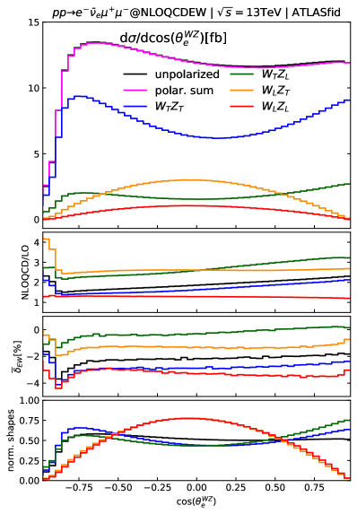
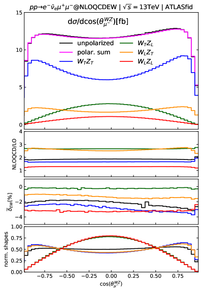
Figure 2: Distributions in $\cos\theta^{WZ}_{e}$ (left) and $\cos\theta^{WZ}_{\mu^{-}}$ (right). These angles are calculated in the $WZ$ center-of-mass system (more details are provided in the text), hence denoted with the $WZ$ superscript. The big panel shows the absolute values of the cross sections at NLO QCD+EW. The middle-up panel displays the ratio of the NLO QCD cross sections to the corresponding LO ones. The middle-down panel shows $\bar{\delta}_{\text{EW}}$, the EW corrections relative to the NLO QCD cross sections, in percent. In the bottom panel, the normalized shapes of the distributions are plotted to highlight differences in shape.

In Fig. 2 we present the differential cross sections in $\cos\theta^{WZ}_{e}$ (left) and $\cos\theta^{WZ}_{\mu^{-}}$ (right). The polar angle $\theta^{WZ}_{\ell}$ is defined as the angle between the momentum of the parent gauge boson calculated in the $WZ$ c.m.s ($\vec{p}^{\text{WZ-cms}}_{V}$) and the momentum of the lepton calculated in the gauge boson rest frame ($\vec{p}^{\text{V-rest}}_{\ell}$). These angles are chosen for our analyses because the electron angle distribution is sensitive to the $W$ boson polarizations, while the muon angle distribution is sensitive to the $Z$ boson polarizations.

In the top panels, we display the NLO QCD+EW differential cross sections for the double polarizations LL (red), LT (orange), TL (green), TT (blue). Their sum is plotted in magenta (only shown in the top panels), while the unpolarized cross section is in black. The difference between the unpolarized and the polarization sum is the interference shown in the last row of Table 1. As seen from these plots, the interference effect is negligible across the full range of the angle for both cases. Similar to the case of $W^{+}Z$, the $W_{T}^{-}Z_{T}$ cross section is largest while the $W_{L}^{-}Z_{L}$ smallest for both distributions. Comparing the $W_{L}^{-}Z_{T}$ to the $W_{T}^{-}Z_{L}$ $\cos\theta^{WZ}_{e}$ distribution, we see that the transverse $W$ mode is more dominant at the edge regions where $|\cos\theta^{WZ}_{e}|\approx 1$, while the longitudinal $W$ cross section is larger in the center region $|\cos\theta^{WZ}_{e}|<0.5$. The same features are observed in the right plot of the muon angle. The depletion at $|\cos\theta^{WZ}_{\mu^{-}}|\approx 1$ in the $W_{T}Z_{T}$ and $W_{L}Z_{T}$ distributions in the right plot is due to the $p_{T}$ and $\eta$ cuts on the muon and anti-muon. These cuts do not affect the shapes of the $W_{T}Z_{L}$ and $W_{L}Z_{L}$ polarizations as observed in Denner:2020eck . Similar results are seen in the left plot, but there is no depletion at $\cos\theta^{WZ}_{e}\approx+1$ because there are no $p_{T}$ and $\eta$ cuts on the neutrino.

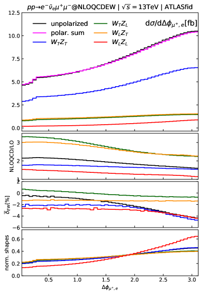
Figure 3: Same as Fig. 2 but for the azimuthal separation between the electron and the muon $\Delta\phi_{\mu^{-},e^{-}}$ (left) and between the electron and the anti-muon $\Delta\phi_{\mu^{+},e^{-}}$ (right).

The ratios of the NLO QCD cross section to the corresponding LO one ($K$-factor) are plotted in the middle-up panel, while the $\bar{\delta}_{\text{EW}}$ corrections are shown in the middle-down panel. The QCD $K$-factor for the $LL$ polarization is the smallest (about $1.3$) and rather flat in the whole range of $\cos\theta^{WZ}_{e}$ while it is larger for the other polarizations, with a sharp rise in the region $\cos\theta^{WZ}_{e}<-0.8$ where there is a stronger depletion of the differential cross section. The $K$-factor is greater than $4$ at $\cos\theta^{WZ}_{e}=-1$ for the $W_{L}Z_{T}$ case. For the muon angle distributions, the QCD $K$-factors are flatter in the whole range, varying from $1.2$ to $2.8$. In the EW correction panels, note that $\bar{\delta}_{\text{EW}}$ is defined with respect to the NLO QCD result, see Eq. (32). The $|\bar{\delta}_{\text{EW}}|$ is smallest for the TT component and largest for the LL component. They remain small in the whole range of $\cos\theta^{WZ}_{\ell}$ and vary from $-4.2\%$ to $0.1\%$.

Finally, in the bottom panels we show the distributions $d\sigma/d\cos\theta$ normalized to their corresponding integrated cross sections presented in Table 1. This helps us to see the differences in shape of the various polarizations. From the $\cos\theta^{WZ}_{e}$ distribution, we observe two distinct shapes: The $W_{L}Z_{L}$ and $W_{L}Z_{T}$ have the same shape with a maximum at $\cos\theta^{WZ}_{e}=0$, while the $W_{T}Z_{L}$ and $W_{T}Z_{T}$ are similar with a minimum at the center. This feature is well expected because the $\cos\theta^{WZ}_{e}$ distribution is sensitive to the polarizations of the $W$ boson and is not much affected by the polarization of the $Z$ boson. The same thing can be said for the $\cos\theta^{WZ}_{\mu^{-}}$ case where the longitudinal and transverse $Z$ bosons produce two different shapes.

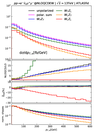
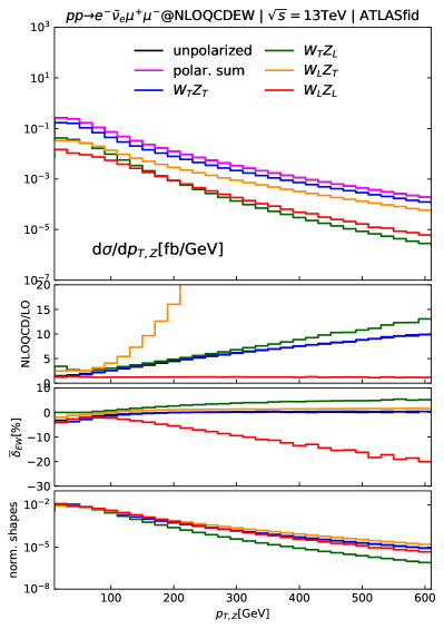
Figure 4: Same as Fig. 2 but for the transverse momentum of the electron (left) and the $Z$ boson (right).

In the same format and color code, we plot in Fig. 3 the distributions in the azimuthal separation between the electron and the muon $\Delta\phi_{\mu^{-},e^{-}}$ (left), between the electron and the anti-muon $\Delta\phi_{\mu^{+},e^{-}}$ (right). All polarizations show an increase in the differential cross section with increasing separation, however the QCD $K$-factors decrease. As in the case of the $\cos\theta^{WZ}_{\ell}$ distributions, the QCD corrections are large while the EW corrections are small, being less than $5\%$ across the full range of $\Delta\phi\in[0,\pi]$. The normalized shape panels show that this distribution can give extra power to separate the LL polarization as it has a different shape from the other polarizations for both the left and the right plots.

The transverse momentum distributions of the electron (left) and of the $Z$ boson (right) are presented in Fig. 4. More clearly than the above angular distributions, these distributions show that the QCD and EW corrections are not the same for different polarizations. QCD correction is largest for the $W_{T}Z_{L}$ in the $p_{T,e}$ distribution, while the $W_{L}Z_{T}$ is largest in the $p_{T,Z}$ one. EW correction is largest for the LL polarization for both distributions. The correction is negative and its magnitude increasing with energy due to the double- and single-Sudakov logarithms in the virtual contribution. Compared to the NLO QCD prediction, the EW correction is $-10\%$ at around $200$ GeV and reaching $-27\%$ at $600$ GeV for the $p_{T,e}$ distribution. For the $p_{T,Z}$ distribution, the correction is smaller, being $-5\%$ at $200$ GeV and $-20\%$ at $600$ GeV. The normalized shapes of the four polarizations are indistinguishable for $p_{T}<100$ GeV and become more diverged at large values.

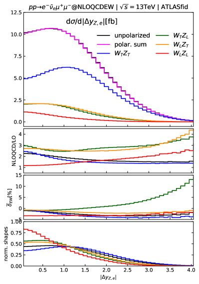
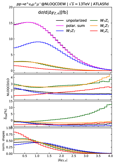
Figure 5: Same as Fig. 2 but for the rapidity separation (in absolute value) between the electron/positron and the $Z$ boson. The left plot is for the process $W^{-}Z$ while the right plot is $W^{+}Z$.

Another interesting distribution which can help to distinguish the doubly longitudinal polarization is the rapidity separation between the electron and the $Z$ boson. This is plotted in Fig. 5 for both the $W^{-}Z$ (left) and $W^{+}Z$ (right) processes. The latter was not shown in Le:2022lrp , hence it is here presented for the sake of comparison. The normalized shape panels show clearly that the LL polarization is different from the other cases. Another remarkable feature is the large EW correction, which increases with large rapidity separation, in the $W_{T}Z_{L}$ polarization. Since the photon-quark induced processes are separated from the photon-radiation processes in our calculation, we can investigate the origin of this large EW correction. We found that it is due to the photon-quark induced processes with an extra jet in the final state. The jet allows for new kinematic configurations such as the jet recoiling against a hard $W$ boson leaving the $Z$ boson the freedom to be soft, or the hard jet recoiling against the $Z$ boson while the $W$ is soft. As shown in Baglio:2013toa , these kinds of configurations can lead to large corrections proportional to $\alpha\log^{2}(p_{T,jet}^{2}/M_{V}^{2})$ ($V=W,Z$). This argument also holds for the gluon-quark induced processes in the QCD corrections. Fig. 5 indeed shows that the QCD corrections are large at large rapidity separation for the $W_{T}Z_{L}$ and $W_{L}Z_{T}$ polarizations. Turning off the gluon-quark induced processes makes this correction significantly smaller. It is interesting to note that while the gluon-quark induced processes affect both the $W_{T}Z_{L}$ and $W_{L}Z_{T}$ polarizations, the photon-quark induced processes increase only the $W_{T}Z_{L}$ case. This reminds us of the difference between QCD and EW corrections.

6 Conclusions

In this paper we have studied the doubly-polarized production of $W^{\pm}Z$ pairs in fully-leptonic channels at the LHC at NLO accuracy for both the QCD and EW corrections. Numerical results for the $W^{+}Z$ process were already presented in the short letter Le:2022lrp . Here we present a detailed description of the calculation method behind the results of Ref. Le:2022lrp and provide further numerical results, mainly for the $W^{-}Z$ process.

The method to calculate NLO QCD corrections for doubly-polarized cross sections in di-boson productions has been established in Denner:2020bcz using the double-pole approximation. NLO EW corrections are more complicated and have been recently calculated in Denner:2021csi for the $ZZ$ process, also in the DPA. In this work, we have extended this method to cover the case of a charged current, namely the $WZ$ process. The method described here can also be straightforwardly used for the $W^{+}W^{-}$ process.

In the numerical result section, we have presented new results for the $W^{-}Z$ process at the NLO QCD+EW level. This has bee done in such a way that the reader can easily compared to the corresponding $W^{+}Z$ results provided in Ref. Le:2022lrp . We note that this is also the first time NLO QCD results for the $W^{-}Z$ process are presented as Ref. Denner:2020eck published only the $W^{+}Z$ NLO QCD results.

Integrated doubly-polarized cross sections have been calculated together with seven-point scale uncertainties. A comparison between our predictions and the new ATLAS measurement ATLAS:2022conf53 has been tabulated and discussed, showing very good agreement within $1.5$ standard deviations. However, the experimental precision is still limited, at the level of tens of percents.

We have presented also differential distributions mainly for the $W^{-}Z$ process together with a detailed analysis of the results. New distributions of the rapidity separation between the electron and the $Z$ boson ($\Delta y_{Z,e}$) have been shown for both $W^{-}Z$ and $W^{+}Z$ processes. The kinematic variables chosen here are those which provide discrimination power to separate different polarizations (mostly lepton angular observables) or those which show the importance of EW corrections (lepton $p_{T}$). We have found that, as in the case of the $W^{+}Z$ channel, EW corrections are most sizable in the $p_{T,e}$ and $p_{T,Z}$ distributions of the doubly-longitudinal polarization in the $W^{-}Z$ channel. It is also found that the rapidity separation $\Delta y_{Z,e}$ can help to single out the LL polarization.

- (1) ATLAS collaboration, G. Aad et al., Search for new phenomena in three- or four-lepton events in collisions at = 13 TeV with the ATLAS detector, Phys. Lett. B 824 (2022) 136832 [2107.00404].
- (2) CMS collaboration, A. Tumasyan et al., Measurement of the inclusive and differential WZ production cross sections, polarization angles, and triple gauge couplings in pp collisions at = 13 TeV, 2110.11231.
- (3) ATLAS collaboration, G. Aad et al., Measurements of differential cross-sections in four-lepton events in 13 TeV proton-proton collisions with the ATLAS detector, JHEP 07 (2021) 005 [2103.01918].
- (4) J. Ohnemus, An order calculation of hadronic production, Phys. Rev. D44 (1991) 3477.
- (5) S. Frixione, P. Nason and G. Ridolfi, Strong corrections to W Z production at hadron colliders, Nucl. Phys. B383 (1992) 3.
- (6) L. J. Dixon, Z. Kunszt and A. Signer, Helicity amplitudes for O(alpha-s) production of , , , , or pairs at hadron colliders, Nucl. Phys. B531 (1998) 3 [hep-ph/9803250].
- (7) L. J. Dixon, Z. Kunszt and A. Signer, Vector boson pair production in hadronic collisions at order : Lepton correlations and anomalous couplings, Phys. Rev. D60 (1999) 114037 [hep-ph/9907305].
- (8) E. Accomando, A. Denner and A. Kaiser, Logarithmic electroweak corrections to gauge-boson pair production at the LHC, Nucl. Phys. B 706 (2005) 325 [hep-ph/0409247].
- (9) A. Bierweiler, T. Kasprzik and J. H. Kühn, Vector-boson pair production at the LHC to accuracy, JHEP 12 (2013) 071 [1305.5402].
- (10) J. Baglio, L. D. Ninh and M. M. Weber, Massive gauge boson pair production at the LHC: a next-to-leading order story, Phys. Rev. D88 (2013) 113005 [1307.4331].
- (11) B. Biedermann, A. Denner and L. Hofer, Next-to-leading-order electroweak corrections to the production of three charged leptons plus missing energy at the LHC, JHEP 10 (2017) 043 [1708.06938].
- (12) T. Gehrmann, A. von Manteuffel and L. Tancredi, The two-loop helicity amplitudes for leptons, JHEP 09 (2015) 128 [1503.04812].
- (13) M. Grazzini, S. Kallweit, D. Rathlev and M. Wiesemann, production at hadron colliders in NNLO QCD, Phys. Lett. B761 (2016) 179 [1604.08576].
- (14) M. Grazzini, S. Kallweit, D. Rathlev and M. Wiesemann, production at the LHC: fiducial cross sections and distributions in NNLO QCD, JHEP 05 (2017) 139 [1703.09065].
- (15) M. Grazzini, S. Kallweit, J. M. Lindert, S. Pozzorini and M. Wiesemann, NNLO QCD + NLO EW with Matrix+OpenLoops: precise predictions for vector-boson pair production, JHEP 02 (2020) 087 [1912.00068].
- (16) T. Melia, P. Nason, R. Rontsch and G. Zanderighi, W+W-, WZ and ZZ production in the POWHEG BOX, JHEP 11 (2011) 078 [1107.5051].
- (17) P. Nason and G. Zanderighi, , and production in the POWHEG-BOX-V2, Eur. Phys. J. C 74 (2014) 2702 [1311.1365].
- (18) M. Chiesa, C. Oleari and E. Re, NLO QCD+NLO EW corrections to diboson production matched to parton shower, Eur. Phys. J. C 80 (2020) 849 [2005.12146].
- (19) M. Chiesa, A. Denner and J.-N. Lang, Anomalous triple-gauge-boson interactions in vector-boson pair production with RECOLA2, Eur. Phys. J. C 78 (2018) 467 [1804.01477].
- (20) J. Baglio, S. Dawson and S. Homiller, QCD corrections in Standard Model EFT fits to and production, Phys. Rev. D 100 (2019) 113010 [1909.11576].
- (21) J. Baglio, S. Dawson, S. Homiller, S. D. Lane and I. M. Lewis, Validity of standard model EFT studies of VH and VV production at NLO, Phys. Rev. D 101 (2020) 115004 [2003.07862].
- (22) J. M. Campbell and R. K. Ellis, An Update on vector boson pair production at hadron colliders, Phys. Rev. D60 (1999) 113006 [hep-ph/9905386].
- (23) J. M. Campbell, R. K. Ellis and C. Williams, Vector boson pair production at the LHC, JHEP 07 (2011) 018 [1105.0020].
- (24) K. Arnold et al., VBFNLO: A Parton level Monte Carlo for processes with electroweak bosons, Comput. Phys. Commun. 180 (2009) 1661 [0811.4559].
- (25) J. Baglio et al., Release Note - VBFNLO 2.7.0, 1404.3940.
- (26) R. Poncelet and A. Popescu, NNLO QCD study of polarised W+W- production at the LHC, JHEP 07 (2021) 023 [2102.13583].
- (27) ATLAS collaboration, M. Aaboud et al., Measurement of production cross sections and gauge boson polarisation in collisions at TeV with the ATLAS detector, Eur. Phys. J. C 79 (2019) 535 [1902.05759].
- (28) ATLAS collaboration, Observation of gauge boson joint-polarisation states in production from collisions at TeV with the ATLAS detector, Tech. Rep. ATLAS-CONF-2022-053, CERN, 2022.
- (29) C. L. Bilchak, R. W. Brown and J. D. Stroughair, and Polarization in Pair Production: Dominant Helicities, Phys. Rev. D29 (1984) 375.
- (30) S. S. D. Willenbrock, Pair Production of and Bosons and the Goldstone Boson Equivalence Theorem, Annals Phys. 186 (1988) 15.
- (31) W. J. Stirling and E. Vryonidou, Electroweak gauge boson polarisation at the LHC, JHEP 07 (2012) 124 [1204.6427].
- (32) J. Baglio and L. D. Ninh, Fiducial polarization observables in hadronic WZ production: A next-to-leading order QCD+EW study, JHEP 04 (2019) 065 [1810.11034].
- (33) J. Baglio and L. D. Ninh, Polarization observables in WZ production at the 13 TeV LHC: Inclusive case, Commun. in Phys. 30 (2020) 35 [1910.13746].
- (34) R. Rahaman and R. K. Singh, Anomalous triple gauge boson couplings in production at the LHC and the role of boson polarizations, Nucl. Phys. B 948 (2019) 114754 [1810.11657].
- (35) R. Rahaman and R. K. Singh, Unravelling the anomalous gauge boson couplings in production at the LHC and the role of spin- polarizations, JHEP 04 (2020) 075 [1911.03111].
- (36) A. Denner and G. Pelliccioli, Polarized electroweak bosons in production at the LHC including NLO QCD effects, JHEP 09 (2020) 164 [2006.14867].
- (37) A. Denner and G. Pelliccioli, NLO QCD predictions for doubly-polarized WZ production at the LHC, Phys. Lett. B 814 (2021) 136107 [2010.07149].
- (38) A. Denner and G. Pelliccioli, NLO EW and QCD corrections to polarized ZZ production in the four-charged-lepton channel at the LHC, 2107.06579.
- (39) D. N. Le and J. Baglio, Doubly-polarized hadronic cross sections at NLO QCD+EW accuracy, 2203.01470.
- (40) A. Denner, S. Dittmaier, M. Roth and D. Wackeroth, Electroweak radiative corrections to in double pole approximation: The RACOONWW approach, Nucl.Phys. B587 (2000) 67 [hep-ph/0006307].
- (41) S. Catani and M. Seymour, A General algorithm for calculating jet cross-sections in NLO QCD, Nucl.Phys. B485 (1997) 291 [hep-ph/9605323].
- (42) S. Dittmaier, A General approach to photon radiation off fermions, Nucl. Phys. B565 (2000) 69 [hep-ph/9904440].
- (43) W. Beenakker, A. P. Chapovsky and F. A. Berends, Nonfactorizable corrections to W pair production, Phys. Lett. B411 (1997) 203 [hep-ph/9706339].
- (44) A. Denner, S. Dittmaier and M. Roth, Nonfactorizable photonic corrections to , Nucl. Phys. B519 (1998) 39 [hep-ph/9710521].
- (45) A. Denner, S. Dittmaier and M. Roth, Further numerical results on nonfactorizable corrections to , Phys. Lett. B429 (1998) 145 [hep-ph/9803306].
- (46) T. Hahn and M. Perez-Victoria, Automatized one-loop calculations in four and D dimensions, Comput. Phys. Commun. 118 (1999) 153.
- (47) T. Hahn, Generating Feynman diagrams and amplitudes with FeynArts 3, Comput.Phys.Commun. 140 (2001) 418.
- (48) L. Basso, S. Dittmaier, A. Huss and L. Oggero, Techniques for the treatment of IR divergences in decay processes at NLO and application to the top-quark decay, Eur. Phys. J. C76 (2016) 56 [1507.04676].
- (49) G. Watt and R. S. Thorne, Study of Monte Carlo approach to experimental uncertainty propagation with MSTW 2008 PDFs, JHEP 08 (2012) 052 [1205.4024].
- (50) J. Gao and P. Nadolsky, A meta-analysis of parton distribution functions, JHEP 07 (2014) 035 [1401.0013].
- (51) L. A. Harland-Lang, A. D. Martin, P. Motylinski and R. S. Thorne, Parton distributions in the LHC era: MMHT 2014 PDFs, Eur. Phys. J. C75 (2015) 204 [1412.3989].
- (52) NNPDF collaboration, R. D. Ball et al., Parton distributions for the LHC Run II, JHEP 04 (2015) 040 [1410.8849].
- (53) J. Butterworth et al., PDF4LHC recommendations for LHC Run II, J. Phys. G43 (2016) 023001 [1510.03865].
- (54) S. Dulat, T.-J. Hou, J. Gao, M. Guzzi, J. Huston, P. Nadolsky et al., New parton distribution functions from a global analysis of quantum chromodynamics, Phys. Rev. D93 (2016) 033006 [1506.07443].
- (55) D. de Florian, G. F. R. Sborlini and G. Rodrigo, QED corrections to the Altarelli-Parisi splitting functions, Eur. Phys. J. C76 (2016) 282 [1512.00612].
- (56) S. Carrazza, S. Forte, Z. Kassabov, J. I. Latorre and J. Rojo, An Unbiased Hessian Representation for Monte Carlo PDFs, Eur. Phys. J. C75 (2015) 369 [1505.06736].
- (57) A. Manohar, P. Nason, G. P. Salam and G. Zanderighi, How bright is the proton? A precise determination of the photon parton distribution function, Phys. Rev. Lett. 117 (2016) 242002 [1607.04266].
- (58) A. V. Manohar, P. Nason, G. P. Salam and G. Zanderighi, The Photon Content of the Proton, JHEP 12 (2017) 046 [1708.01256].
- (59) A. Buckley, J. Ferrando, S. Lloyd, K. Nordström, B. Page, M. Rüfenacht et al., LHAPDF6: parton density access in the LHC precision era, Eur. Phys. J. C75 (2015) 132 [1412.7420].
- (60) ATLAS collaboration, M. Aaboud et al., Measurement of the boson pair-production cross section in collisions at TeV with the ATLAS Detector, Phys. Lett. B762 (2016) 1 [1606.04017].