Quantifying the homology of periodic cell complexes

Abstract

A periodic cell complex, $K$, has a finite representation as the quotient space, $q(K)$, consisting of equivalence classes of cells identified under the translation group acting on $K$. We study how the Betti numbers and cycles of $K$ are related to those of $q(K)$, first for the case that $K$ is a graph, and then higher-dimensional cell complexes. When $K$ is a $d$-periodic graph, it is possible to define $\mathbb{Z}^{d}$-weights on the edges of the quotient graph and this information permits full recovery of homology generators for $K$. The situation for higher-dimensional cell complexes is more subtle and studied in detail using the Mayer-Vietoris spectral sequence.

1 Introduction

Spatially periodic point patterns arise naturally as models of atomic positions in crystalline materials, and as a tractable way to simulate many interacting objects without the influence of boundary effects. Although simulations using periodic boundary conditions treat points as located in a flat $d$-dimensional torus, the structure being modelled is really some large finite domain built from many copies of a unit cell and thus a subset of $\mathbb{R}^{d}$.

Given the increasing usefulness of persistent homology in many application areas, particularly materials science, the following questions naturally arise.

1. Is the persistence diagram of an infinite crystalline structure well-defined, since the persistent homology of most crystalline structures will not be q-tame, which is usually a minimum requirement for the existence of persistence diagrams [9].

2. How to normalise the persistence diagram of an infinite crystalline structure so that it is independent of the unit cell used.

3. How to approximate the persistence diagram for a large finite domain of a periodic point pattern in $\mathbb{R}^{d}$ given a periodic unit cell embedded in a flat $d$-torus.

Physical intuition from more familiar geometric properties suggests that we should be able to normalise the number of points in a persistence diagram by the volume of the domain in $\mathbb{R}^{d}$ to obtain a quantity that is independent of domain size. This is exactly how we define the porosity of a material for example: as the volume of solid matter normalised by the volume of the domain. However, this type of normalisation is appropriate only when working with what physicists term an extensive property; a quantity $f$ that satisfies the properties of a valuation, most notably the inclusion-exclusion formula $f(A\cup B)=f(A)+f(B)-f(A\cap B)$. It is easy to show that the Betti number invariants of homology $\beta_{i}$, and consequently the persistence diagrams, are not valuations. For example, two $\sqsubset$-shaped domains that overlap to form a square annulus have $\beta_{i}(\sqsubset)+\beta_{i}(\sqsupset)\neq\beta_{i}(\square)+\beta_{i}(^{-}_{-})$, for $i=0,1$.

Given that there is this fundamental obstruction to a simple normalisation procedure for persistence diagrams, the current paper begins the process of providing an answer to the above questions by studying the homology of periodic cell complexes. We are particularly motivated by peculiar behaviour in the topology of finite presentations of these complexes, such as two disconnected interwoven graphs over cubical lattices projecting onto a single connected quotient graph as in Figure 1 below. We present a detailed study of how the Betti numbers of a finite cell complex (the quotient space) are related to those of its infinite periodic cover, $K$.

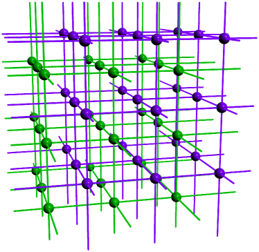
Figure 1: A section of two interwoven cubical lattices along integer and half integer coordinates in $\mathbb{R}^{3}$ (with connected components coloured green and purple) and its weighted quotient graph with respect to translations in the directions $(\frac{1}{2},\frac{1}{2},\frac{1}{2})$, $(\frac{1}{2},-\frac{1}{2},\frac{1}{2})$ and $(1,0,0)$.

The case of a periodic 1-dimensional cell-complex in $\mathbb{R}^{d}$ i.e., a periodic graph, is considerably simpler than the general $k$-dimensional case, and has well studied representations [12, 5, 14]. Results about the number of connected components ($\beta_{0}$) of periodic graphs can be found in computer science, electronics, crystallography and graph theory literature [13, 11, 1, 25]. We rephrase these results in Section 3 using the terminology of chain complexes and homology so that we can study the generalisation to higher dimensions. In short, a periodic graph with undirected edges is mapped to the quotient space built from translational equivalence classes of vertices and edges (see Figure 1). This finite quotient graph can be given $d$-dimensional vector weights that encode a translational offset between the vertex representatives at each end of the oriented edge. The number of components of the infinite periodic graph is then determined by comparing the span of the vector weights with the unit lattice basis for $\mathbb{R}^{d}$.

In Section 4 we then look at $k$-dimensional periodic cell-complexes, $k\geq 2$, and discuss how there is no simple method analogous to the vector weights on edges for encoding the translational offsets of boundaries of $k$-cells. With no simple generalistations of the formulae derived for periodic graphs, this means we have trouble distinguishing cycles in $K$ from cycles in its quotient. We instead look at successively larger (but still periodic) finite domains, $X$, and establish a method to identify toroidal or open cycles that are due to the periodic boundary conditions and do not lift to cycles in the infinite periodic structure $K$. This involves application of the Mayer-Vietoris spectral sequence, which we introduce in Section 5, and enables us to identify and classify true cycles of $K$ and impose an approximate lower bound for the size of $X$ required to view these features.

Our results are motivated by application to the analysis of crystal structures, where we have a periodic point cloud in space (i.e., atom positions) and a fixed cellular complex where edges represent bonds and higher dimensional cells represent higher order atomic interactions. Persistent homology is another natural tool for studying topological and geometric structure of periodic point clouds. Although we focus on regular homology in this paper, we will note when a result can be adjusted to the case of persistent homology.

1.1 Related Work

In Section 3 we define the notion of a weighted quotient graph. The definition we employ agrees with the “vector method” introduced in [10], to which we direct the reader for more details. In recent years, weighted quotient graphs have been studied extensively and become ubiquitous with structure classification in topological crystallography (c.f., [12, 14]), where they are known as labelled quotient graphs). A weighted quotient graph is also referred to as a static graph in a discrete mathematical setting (c.f., [17, 11]) where it is used to model Very Large Scale Integration and dynamic optimisation problems (see [18, 23]). In this setting, the periodic graph is called the dynamic graph constructed by interpreting edge weights as shift vectors which generate translational symmetries.

In Section 3 we present Theorem 3.3 which relates the homology of a periodic graph to properties of its weighted quotient graph. The 0-dimensional result was first derived in [11] in the language of electronics and computer science and was independently reformulated in the language of graph theory in Corollary 1.9.3 of [13] and Theorem 3.6 of [1] to prove an analogous result for any action on a connected graph. We rephrase and provide a new proof from our perspective in the language of algebraic topology, and use these methods to generalise to 1-dimensional homology, which we believe to be an original result. Theorems 6.2 and  6.3 of [25] use similar techniques as in our proof of Theorem 3.3. However, their analysis of these results focuses on categorical properties and classifications of quotient graphs, whereas we focus on an explicit construction of the homology of the infinite cover.

In the case of a 1-periodic cell complex $K$ (of arbitrary dimension) we may think of the map $K\to q(K)$ sending $K$ to its quotient space $q(K)$ of translational equivalence classes as being equivalent to a map $K\to\mathbb{S}^{1}$. This case has been well-studied with Novokov homology [22] which generalises the methods of Morse theory, allowing one to explicitly calculate the homology of $K$ over the field of Laurent power series. A computer-friendly method to calculate this with Jordan blocks is described in [7].

The Mayer-Vietoris spectral sequence (MVSS) was first used in topological data analysis to localise low-dimensional cycles of a topological space [26]. More recently, it has been presented primarily as a method for parallelising persistent homology calculations of large data sets (c.f. [21, 4]) and has been implemented for abstract simplicial complexes [20]. In [16] they use a persistence version of the MVSS to prove an approximate nerve theorem for persistence diagrams. Computer implementations of a persistence Mayer-Vietoris spectral sequence can be found in [19, 8], although these encounter what [16] refer to as the “extension problem”, which we briefly discuss in Section 5.1. It is also well-known that persistent homology can be calculated through the spectral sequence of a filtration (c.f. [3, 2]). However, none of these applications have yet been used to study periodic spaces.

2 Notation

This section covers basic definitions and sets up our notation for the objects studied in this paper.

2.1 Periodic Spaces and Unit Cells

A $d$-periodic complex, $K$, in $\mathbb{R}^{l}$ is a cell complex which permits a free action by a free abelian group $T$ of rank $d\leq l$, so that $T$ has a basis of $d$ automorphims $\mathbf{t}_{1},\dots,\mathbf{t}_{d}:K\to K$. Throughout this paper, we assume $K$ contains countably many cells and that $T$ acts on $K$ by translations, so that the $\mathbf{t}_{i}$ are geometrically realised as $d$ linearly independent translations in $\mathbb{R}^{l}$.

A unit cell, $U\subset K$, contains a representative of each equivalence class of cells in $K/T$, where $K/T:=K/\sim$ for the equivalence relation $a\sim b$ if $b=\mathbf{t}(a)$ for some $\mathbf{t}\in T$. $U$ is in general not a subcomplex of $K$, however $\{\mathbf{t}(U)\,:\,\mathbf{t}\in T\}$ partitions $K$. We call the smallest subcomplex of $K$ containing $U$ the closure of $U$ and denote it by $\overline{U}$. In addition, we assume in this paper that $\overline{U}$ is finite, although this distinction is only necessary for Theorem 4.3. Finally, a fundamental domain for $T$ is a convex subset $D\subset\mathbb{R}^{l}$ such that the projection $D\to\mathbb{R}^{l}/T$ is a bijection. It is always possible to choose $U$ so that the vertex representatives of $K/T$ belong to a fundamental domain for $T$.

We say $Y$ is constructed from $n_{1}\times\cdots\times n_{d}$ copies of $U$ if $Y$ is the smallest subcomplex of $K$ containing $\bigcup_{c_{1},\dots,c_{d}=0}^{n-1}(\sum_{i=1}^{d}c_{i}\mathbf{t}_{i})(U)$. We say $X$ is constructed from $n_{1}\times\cdots\times n_{d}$ copies of $U$ with periodic boundary conditions if $X=Y/\sim$ where $a\sim b$ if $a=\mathbf{t}(b)$ for some $\mathbf{t}\in\langle n_{1}\mathbf{t}_{1},\dots,n_{d}\mathbf{t}_{d}\rangle$ (here angle brackets denote the span). Equivalently, $X=K/\widetilde{T}$ for the subgroup $\widetilde{T}=\langle n_{1}\mathbf{t}_{1},\dots,n_{d}\mathbf{t}_{d}\rangle$ of $T$.

2.2 Homology and the Fundamental Group

For an abelian group $G$ we denote that $N$ is a subgroup of $G$ by $N<G$ or $N\leq G$. For some $N\leq G$, recall that the index of $N$ in $G$ is the cardinality of the quotient group $G/N$ and we denote this by $[G:N]$.

Given a cell complex $K$, $\pi_{1}(K,v)$ denotes the fundamental group of $K$ with basepoint at $v$. If the choice of basepoint is understood or is arbitrary (up to connected component), then we will write $\pi_{1}(K)$.

We recall that the chain complex of $K$, $C_{\bullet}(K,G)$, is the differential $\mathbb{Z}$-graded module where $C_{k}(K,G)$ is the free $G$-module whose basis is the oriented $k$-cells of $K$ and whose boundary map $\partial$ sends a $k$-cell to the sum of its boundary $(k-1)$-cells. If there are infinitely many $k$-cells, $C_{k}(K,G)$ contains only finite oriented $G$-sums of $k$-cells. We will write $C_{\bullet}(K,G)=C_{\bullet}(K)$ whenever $G$ is understood. We denote $Z_{\bullet}(K):=\ker(\partial)$ to be the cycles of $K$ and $B_{\bullet}(K):=\operatorname{im}(\partial)$ to be the boundaries of $K$. The fundamental result of homology, $\partial\partial=0$, tells us that $B_{\bullet}(K)<Z_{\bullet}(K)$, and the cellular homology of $K$ is then $H_{\bullet}(K):=Z_{\bullet}(K)/B_{\bullet}(K)$. The $k^{\mathrm{th}}$ Betti number of $K$ (with respect to $G$) is the rank of the free part of $H_{k}(K)$.

Throughout, we also assume standard concepts and results from algebraic topology and linear algebra such as covering spaces, homotopy equivalence, and the rank-nullity theorem.

3 Periodic Graphs

In this section, $K$ denotes a $d$-periodic simplicial complex with only $0$- and $1$-dimensional cells (a graph) embedded in $\mathbb{R}^{l}$. We assume a group $T\cong\mathbb{Z}^{d}$ of vectors acts freely on $K$ by translations, and let $q:K\to q(K):=K/T$ denote the canonical quotient map. Further, chain complexes and homology groups are understood to have coefficients in $\mathbb{Z}$.

3.1 Weighted Quotient Graphs

We start by defining the weight of an edge in $q(K)$ as the translation offset between end points of its lift in $K$.

Definition 3.1.

Weighted quotient graph (WQG). For each equivalence class of edge $e\in q(K)$, we define a weight $w(e)\in T$ as follows.

1. Enumerate the vertices of $q(K)$. When $i\leq j$, any edge joining $v_{i}$ and $v_{j}$ in $q(K)$ is given the direction pointing from $v_{i}$ to $v_{j}$.

2. For each vertex $v_{i}\in q(K)$ choose a fixed representative $\tilde{v}_{i}\in q^{-1}(v_{i})$. Then each vertex $a\in K$ can be written uniquely as $a=\mathbf{t}_{a}(\tilde{v}_{i})$ for some $i$ and $\mathbf{t}_{a}\in T$.

3. Each edge $(a,b)\in K$ therefore joins $\mathbf{t}_{a}(\tilde{v}_{i})$ and $\mathbf{t}_{b}(\tilde{v}_{j})$. Swapping the order of $a$ and $b$ if necessary we assume $i\leq j$. Now define $w(e)=w((v_{i},v_{j}))=w([(a,b)])=\mathbf{t}_{b}-\mathbf{t}_{a}$.

Observe that $w([(a,b)])=\mathbf{t}_{b}-\mathbf{t}_{a}$ is independent of the choice of representative $(a,b)$ from $q^{-1}((v_{i},v_{j}))$ because any other representative is a translated copy of this one. Given a basis for $T$, we can write $w(e)$ as an integer vector of coefficients in $\mathbb{Z}^{d}$.

WQG’s are not uniquely determined by $K$, as $q(K)$ depends on the choice of $T$ (which is not necessarily maximal) and the edge weights depend on the choice of vertex representatives $\tilde{v}_{i}\in K$. However, in any WQG we can extend the domain of $w$ to be any directed path of edges in $q(K)$. Explicitly, for a path $p$ along the directed edges $e_{1},\dots,e_{m}$ we define $w(p)=\sum_{i=1}^{m}w(e_{i})$ and $w(p^{-1})=-w(p)$ (where $p^{-1}$ denotes the reverse of the path $p$ in $q(K)$). This means $w$ takes the same value on homotopy-equivalent egde-paths and it restricts to a group homomorphism $w:\pi_{1}(q(K),v)\to\mathbb{Z}^{d}$ for any basepoint $v$. From a homological perspective, we may also consider $w$ a $T$-valued cocycle of $q(K)$.

Definition 3.2.

Let $Q$ be a connected WQG with weights given as $\mathbb{Z}^{d}$-coefficients. We set $W_{Q}$ to be the subgroup of $\mathbb{Z}^{d}$ containing weights of all cycles in $q(K)$,

$$W_{Q}:=\langle w(\ell)\,:\,\ell\text{ is a cycle in }Q\rangle$$

The subgroup $W_{Q}$ is independent of choice of basepoint, so we see that

$$W_{Q}=\operatorname{im}\left(w:\pi_{1}(Q)\to\mathbb{Z}^{d}\right).$$

Connectivity of $q(K)$ does not guarantee that $K$ is connected, as the example of Fig. 1 shows. The index of $W_{q(K)}$ in the original lattice group $T=\mathbb{Z}^{d}$ will tell us the number of path-connected components of $K$. Also, since $w(p)$ encodes the relative offset in $K$ between endpoints of a path $p$ in $q(K)$, we see that if $p$ is a cycle in $q(K)$ with $w(p)=0$, then the lift $q^{-1}[p]$ in $K$ contains elements of $Z_{1}(K)$. These concepts are the basis of the following result.

Theorem 3.3.

Suppose $q(K)=\sqcup_{i=1}^{N}Q_{i}$ is a WQG of $\varepsilon$ edges and $\nu$ vertices, decomposed into $N$ connected components, $Q_{i}$. Then

1. $H_{0}(K)$ has a basis of $\sum_{i=1}^{N}\,[\mathbb{Z}^{d}:W_{Q_{i}}]$ elements.

2. $H_{1}(K)$ is generated by $\varepsilon-\nu+N\binom{d-1}{2}$ homology classes up to translation.

Moreover, $q(K)$ has sufficient information to construct a generating set of $H_{\bullet}(K)$.

In Section 3.2 we illustrate the proof of Theorem 3.3 for the case of the $2$-periodic Kagome lattice.

Proof.

(1) Disconnected subgraphs of $q(K)$ will have disconnected lifts, so without loss of generality we may assume $q(K)$ is connected Let $v_{1},\dots,v_{k}$ be the vertices of $q(K)$ whose representatives are $\tilde{v}_{1},\dots,\tilde{v}_{k}$ in $K$. Since $q(K)$ is connected, each vertex $v_{2},\dots,v_{k}$ is homologous to $v_{1}$ And $q:K\to q(K)$ is a covering space, so any path in $q(K)$ has a unique lift up to the choice of basepoint, so every vertex of $q^{-1}(\{v_{2},\dots,v_{k}\})$ is homologous to a vertex of $q^{-1}(v_{1})$. Furthermore, if there is a cycle of weight $\mathbf{t}\in\mathbb{Z}^{d}$ about $v_{1}$ then for any $\mathbf{s}\in T$ this lifts to a unique path from $\mathbf{s}(\tilde{v}_{1})$ to $(\mathbf{t}+\mathbf{s})(\tilde{v}_{1})$. Conversely, by translational symmetry of $K$ any path from $\tilde{v}_{1}$ to $\mathbf{t}(\tilde{v}_{1})$ corresponds to a unique path from $\mathbf{s}(\tilde{v}_{1})$ to $(\mathbf{t}+\mathbf{s})(\tilde{v}_{1})$ and projects onto a cycle of weight $\mathbf{t}$. Hence $\mathbf{t}(\tilde{v}_{1})$ and $\mathbf{s}(\tilde{v}_{1})$ are homologous if and only if $\mathbf{s}+W_{q(K)}=\mathbf{t}+W_{q(K)}$ as cosets. Thus each generator of $H_{0}(K)$ is represented by $\tilde{v}_{1}$, offset by a translation in $\mathbb{Z}^{d}/W_{q(K)}$.

(2) As above, we may assume $q(K)$ is connected. Let $v_{1}$ and $\tilde{v}_{1}$ be as above. $H_{1}(K)$ can be identified with the abelianisation of $\pi_{1}(K,\tilde{v}_{1})$, with additional translated copies for each connected component of $K$, so it suffices to find the generators of $\pi_{1}(K,\tilde{v}_{1})$. The quotient map $q:K\to q(K)$ is a covering space so $q^{*}:\pi_{1}(K,\tilde{v}_{1})\hookrightarrow\pi_{1}(q(K),v_{1})$, where the image $q^{*}(\pi_{1}(K,\tilde{v}_{1}))$ contains the homotopy classes of zero-weight cycles based at $v_{1}\in q(K)$.

We construct generators of $\pi_{1}(K,\tilde{v}_{1})$ by building $q(K)$ from a spanning tree and identifying all cycles of weight zero created as each additional edge is added. A chosen spanning tree $F_{0}$, lifts to a collection of disconnected trees $q^{-1}(F_{0})\subset K$. Adding another edge of $q(K)$ to $F_{0}$ creates a generator of $\pi_{1}(q(K),v_{1})$ which lifts either to (translated copies of) a closed circuit in $K$ or to a path from $\tilde{v}_{1}$ to $\mathbf{t}(\tilde{v}_{1})$. We proceed as follows to determine the implication for $q^{*}(\pi_{1}(K,\tilde{v}_{1}))$.

1. Inductively for $i=1,\dots,d$, if the addition of an edge $e$ to $F_{i-1}$ has the property that $[W_{F_{i-1}\cup\{e\}}\,:\,W_{F_{i-1}}]=\infty$ then choose a new cycle $p_{i}$ through $v_{1}$ such that $\langle w(p_{j})\,|\,j<i\rangle$ is a basis for $F_{i-1}\cup\{e\}$. We record $p_{i}$, $w(p_{i})$ and construct $F_{i}:=F_{i-1}\cup\{e\}$.

2. For each $j=1,\dots,\varepsilon-d-\nu+1$, pick any edge $e$ in $q(G)\backslash F_{j+d-1}$ and choose a new cycle $\ell_{j}$ through $v_{1}$ in $F_{j+d-1}\cup\{e\}$ which satisfies the property that $\{w(p_{k})\,:\,k=1,\dots,d\}\cup\{w(\ell_{k})\,:\,k=1,\dots,j\}$ generates $W_{F_{j+d-1}}$. We record $\ell_{j}$, $w(\ell_{j})$ and construct $F_{j+d}=F_{j+d-1}\cup\{e\}$.

In Step 1, the condition $[W_{F_{i-1}\cup\{e\}}\,:\,W_{F_{i-1}}]=\infty$ ensures the existence of some $p_{i}$ such that $\langle w(p_{j})\,|\,j<i\rangle$ is a basis for $F_{i}=F_{i-1}\cup\{e\}$. Each $p_{i}$ will lift to a collection of infinite paths through $K$ in independent directions, and the fact that $\beta_{0}(K)=[\mathbb{Z}^{d}:W_{q(K)}]<\infty$ means $w(p_{1}),\cdots,w(p_{d})$ will be a basis for a finite index subspace of $W_{q(K)}$. These properties also ensure that all cycles of length zero in $\pi_{1}(F_{d},v_{1})$ have a minimal generating set of cycles of the form $p_{i}^{-1}[p_{j},p_{k}]p_{i}$ (where $[p_{j},p_{k}]$ denotes the commutator of $p_{j}$ and $p_{k}$, given by $p_{j}^{-1}p_{k}^{-1}p_{j}p_{k}$) for $j\neq k$. There are $\binom{d}{2}$ of these up to conjugation.

In Step 2, each edge in $q^{-1}(e)$ added to $K$ introduces a single generator to $\pi_{i}(F_{j+d-1},\tilde{v}_{1})$, and the translational symmetry of $K$ ensures these cycles are identical up to path conjugation. Explicitly, since $[\mathbb{Z}^{d}\,:\,F_{j+d-1}]\leq[\mathbb{Z}^{d}\,:\,F_{d}]<\infty$ there is some $N\in\mathbb{N}$ such that $N\cdot w(\ell_{j})=\sum_{k=1}^{d}c_{k}w(p_{k})+\sum_{k=1}^{j-1}d_{k}w(\ell_{k})$. Thus $p_{d}^{-c_{d}}\cdots p_{2}^{-c_{2}}p_{1}^{-c_{1}}\ell_{j-1}^{-d_{k}}\cdots\ell_{1}^{-d_{1}}\ell_{j}^{N}$ will be a cycle of weight zero in $q(K)$ (where we read each path from right to left) and we think of each $\ell_{j}^{N}$ as lifting to a collection of shortcuts through the lattice network of $K$. In this step we add $|\{\ell_{j}\}|=\varepsilon-d-\nu+1$ such cycles, since $F_{0}$ has $v-1$ edges, Step 1 adds $d$ edges, and $q(K)=F_{\varepsilon-\nu+1}$ has $\varepsilon$ total edges.

Conjugation by cycles of non-zero weight in $q(K)$ lifts to conjugation by paths in $K$, which amounts to translation when abelianised, so generators of $H_{1}(K)$ can be constructed from translations of lifts of the above cycles. The former collection contributes $\binom{d}{2}$ such generators and the latter contributes $\varepsilon-\nu+1-d$, and the result follows. ∎

Theorem 3.3 allows us to construct the homology of a periodic graph from only the information of a single weighted quotient graph, thus any and all information about its topology can be studied in a finite setting. Moreover, the quantity $\beta_{0}(K)=\sum_{i=1}^{N}\,[\mathbb{Z}^{d}:W_{Q_{i}}]$ is an algebraic invariant among all WQG’s of $K$ and could be used to extend the classification of WQG’s outlined in [12]. However, the number of translation-independent generators for $H_{1}(K)$, $\varepsilon-\nu+N\binom{d-1}{2}$, will vary with the choice of translation group used to form the WQG. If $T^{\prime}<T$ is used to form $q^{\prime}(K)$ then the value of $\varepsilon-\nu$ will in general increase by $O([T:T^{\prime}])$, and the value of $N$ (the number of components of $q(K)$) may fluctuate if $K$ is not connected.

Another issue with Theorem 3.3 is the inability to experimentally verify the results, as all simulations and computations of periodic structures can only be done for finite representations. In practice, periodic structures are studied by taking $n_{1}\times\cdots\times n_{d}$ unit cells with periodic boundary conditions and determining behaviour as $n_{i}\to\infty$. This introduces toroidal properties in the topology, as with WQG’s, but benefits from locally approximating the infinite cover with increasing precision. The methods used to prove Theorem 3.3 easily translate into such finite settings.

Corollary 3.4.

Suppose $X$ is the graph constructed from $n_{1}\times\cdots\times n_{d}$ translated copies of a unit cell of $K$ with periodic boundary conditions, and let $q(K)=\sqcup_{i=1}^{N}Q_{i}$ be a WQG with $\varepsilon$ edges and $\nu$ vertices. Then

1. $$\beta_{0}(X)=\sum_{i=1}^{N}\left[\mathbb{Z}^{d}/\prod_{j=1}^{d}n_{j}\mathbb{Z}\,:\,W_{Q_{i}}/\prod_{j=1}^{d}n_{j}\mathbb{Z}\right]$$

2. $$\beta_{1}(X)=(\varepsilon-\nu)n_{1}\cdots n_{d}+\sum_{i=1}^{N}\left[\mathbb{Z}^{d}/\prod_{j=1}^{d}n_{j}\mathbb{Z}\,:\,W_{Q_{i}}/\prod_{j=1}^{d}n_{j}\mathbb{Z}\right]$$

Moreover, $q(K)$ has sufficient information to construct a generating set of $H_{\bullet}(X)$.

Proof.

(1) follows by analogy from the proof of Statement 1 of Theorem 3.3, and hence will also construct $H_{0}(X)$. (2) follows by equating

$$\chi(X)=\sum_{i=0}^{\infty}(-1)^{i}\beta_{i}(X)=\sum_{i=0}^{\infty}(-1)^{i}\dim\,C_{i}(X)$$

where $\chi(X)$ is the Euler characteristic. Finally, the construction of $H_{1}(X)$ is analogous to the method of proof for Statement 2 of Theorem 3.3, noting that for each $p_{i}$ identified there will be some $N\in\mathbb{N}$ which makes $p_{i}^{N}$ a cycle and some generators of $H_{1}(X)$ identified will be redundant. ∎

3.2 Kagome Lattice Example

Here we provide an illustrated example for the proof of Theorem 3.3 with the 2-periodic Kagome lattice $K_{G}$, shown in Figure 2 alongside one of its weighted quotient graphs $q(K_{G})$.We assume only $q(K_{G})$ is given and we are using Theorem 3.3 to reconstruct the homology of $K_{G}$. For illustrative purposes we use the known structure of $K_{G}$ to depict the construction of the spanning tree and homology generators.

Figure 2: A section of the Kagome lattice (left) and a choice of weighted quotient graph (right) with respect to the translational basis in blue and labelled representative vertices.

We define $e_{ij}$ and $f_{ij}$ to be the edges between $v_{i}$ and $v_{j}$ of zero and non-zero weight respectively in the weighted quotient graph $q(K_{G})$. The cycles $f_{13}^{-1}e_{13}$ and $f_{12}^{-1}e_{12}$ have weights $(1,0)$ and $(0,1)$ respectively, so their weights generate $W_{q(K_{G})}=\mathbb{Z}^{2}$. The procedure in Theorem 3.3 then suggests $\beta_{0}(K_{G})=1$ and the single generator of $H_{0}(K_{G})$ is represented by $\tilde{v}_{1}$. That is, the Kagome lattice clearly has one connected component (connected to $\tilde{v}_{1}$).

Moreover, since $K_{G}$ is 2-periodic and $q(K_{G})$ is connected with six edges and three vertices we can conclude that $H_{1}(K_{G})$ has three generators up to translation. To construct these generators, we first choose a spanning tree of $q(K_{G})$; for example, take the subgraph with only the edges $e_{12}$ and $e_{23}$. We consider the spanning tree and the corresponding lift to $F_{0}\subset N$ below.

We then include the edge $f_{12}$ since $p_{1}=f_{12}^{-1}e_{12}$ is a cycle of weight $(0,1)$ passing through $v_{1}$. The addition of this edge creates an oblique vertical path through the lattice network when lifting to $F_{1}\subset K_{G}$ below, with only trivial cycles.

Next, we add the edge $f_{13}$ since $p_{2}=f_{13}^{-1}e_{23}e_{12}$ is a cycle passing through $v_{1}$ of weight $(1,0)$, not spanned by the weight of $p_{1}$. The addition of this edge lifts to a collection of infinite horizontal paths through the Kagome lattice, in addition to the oblique vertical paths created in the first step. This introduces a single type of cycle (up to translation and concatenation) in $F_{2}$ formed by lifting the commutator of $p_{1}$ and $p_{2}$

$$p_{2}^{-1}p_{1}^{-1}p_{2}p_{1}=e_{12}^{-1}e_{23}^{-1}f_{13}e_{12}^{-1}f_{12}f^{-1}_{13}e_{23}e_{12}f_{12}^{-1}e_{12}.$$

The corresponding $1$-cycle in $K_{G}$ is highlighted in red below. Moreover, the weights of $p_{1}$ and $p_{2}$ span $W_{q(K_{G})}=\mathbb{Z}^{2}$ and so this lift must now be connected. More generally the fact that $[\mathbb{Z}^{2}:W_{q(K_{G}}]<\infty$ at this stage indicates we have finished connecting the lattice framework, and the addition of the remaining edges to $q(K_{G})$ will create additional cycles in $K_{G}$ which are not simply a consequence of the periodicity of the graph.

Now, we include $e_{13}$ to the quotient graph and consider the cycle $\ell_{1}=e_{13}^{-1}e_{23}e_{12}$. This cycle satisfies $w(\ell_{1})=(0,0)$, so $\ell_{1}$ lifts to a unique cycle in $T_{3}\subset K_{G}$ (up to translation) whose corresponding cycle is again shown below in red.

The final addition of $f_{23}$ to complete $T_{4}=q(K_{G})$ adds a cycle $\ell_{2}=e_{13}^{-1}f_{23}e_{12}$ with $w(\ell_{2})=(-1,1)$. Thus

$$p_{2}^{-1}p_{1}\ell_{2}=e_{12}^{-1}e_{23}^{-1}f_{13}f_{12}^{-1}e_{12}e_{13}^{-1}f_{23}e_{12}$$

will lift to create a new type of cycle in $K_{G}$ indicated in red below.

The choice of edges and cycles were not necessarily efficient at times to emphasise how this procedure works independent of such choice, and can be tailored to study persistence or to optimise computational time if desired.

3.3 Interwoven Cubical Lattices Example

Here we again look at the interwoven cubical lattices and illustrate the results of Theorem 3.3 and Corollary 3.4 with two different WQG’s. This shows that despite having a deterministic formula, the betti numbers identified are neither invariant nor do they necessarily behave nicely with $n$.

We have seen that interwoven cubical lattices, $K_{L}$, in Figure 1 admit a connected weighted quotient graph $B$ with respect to translations generated by the basis $\{\left(\frac{1}{2},\frac{1}{2},\frac{1}{2}\right),\left(\frac{1}{2},-\frac{1}{2},\frac{1}{2}\right),(0,0,1)\}$. However, with respect to the standard translational basis of $\mathbb{R}^{3}$ the weighted quotient graph $D$ is no longer connected and takes the other form shown in Figure 3.

Figure 3: The connected WQG $q_{1}(K_{L})=B$ (in black) and the disconnected WQG (coloured according to the connected components in Figure 1).

$D$ respects the connected components of $K_{L}$ at the cost of recording twice as many vertices, edges and weights as $B$, so comparing the two WQG’s is a microcrosm for applications where one might require smaller storage space at the expense of accurate geometry or topology. Using the tools we have constructed, we shall compare and contrast the topology of $K_{L}$ which we can gather from each WQG.

It is clear that $W_{B}=\langle(1,-1,0),(1,1,-1),(0,0,1)\rangle$, which has two cosets in $\mathbb{Z}^{3}$ – namely $W_{B}$ and $(1,0,0)+W_{B}$. Thus $B$ tells us that $\beta_{0}(K_{L})=2$, and the two generators of $H_{0}(K_{L})$ will be represented by $[\tilde{v}]$ and $[\mathbf{t}_{1}(\tilde{v})]$ where $\mathbf{t}_{1}$ indicates translation by $(1/2,1/2,1/2)$.

On the other hand, decomposing $D=D_{1}\sqcup D_{2}$ into two identical connected components, we see that $W_{D_{1}}=W_{D_{2}}=\mathbb{Z}^{3}$ is index $1$ in $\mathbb{Z}^{3}$. So $\beta_{0}(K_{L})=2$ where the generators of $H_{0}(K_{L})$ are given by the representative of the lift of each vertex. Thus both $B$ and $D$ will recover exactly the same results about the 0-dimensional homology, albeit the latter is somewhat more direct.

Next, $B$ has three edges, one vertex, a single connected component and $K_{L}$ is 3-periodic, so there will be three generators of $H_{1}(K_{L})$ identified by $B$ up to translation. Following the same procedure as we used for the Kagome lattice, choosing $p_{1},p_{2},p_{3}$ to simply be the edges of $B$, the generators are identified to be the $1$-cycles corresponding to the lift of paths $p_{2}^{-1}p_{1}^{-1}p_{2}p_{1}$, $p_{3}^{-1}p_{1}^{-1}p_{3}p_{1}$ and $p_{3}^{-1}p_{2}^{-1}p_{3}p_{2}$ (the commutators of $p_{1},p_{2},p_{3}$) to $K_{L}$. These cycles are exactly the squares which appear when fixing one coordinate value, and we consider cycles to be identical to their translated copies on the other connected component.

On the other hand, since $D$ has six edges, two vertices and two connected components, there will instead be six generators of $H_{1}(K_{L})$ up to translation identified by $D$. Following the same process as for $B$ will identify the same cycles as generators – the squares which appear when fixing one coordinate – although the cycles on the green and purple component are no longer considered equivalent up to translation. This is obviously less compact, but there may be physical significance in distinguishing between the two components in application.

We note, however, the generating set of 1-cycles identified by Theorem 3.3 for either quotient graph contains degenerate terms. In the 1-skeleton of the $3$-dimensional cube $C_{3}$, it is well known that five square faces form a basis for $H_{1}(C_{3})$ and the sixth square face can be written as a sum of the remaining five. In the same way, we note that the square face obtained by lifting $p_{1}^{-1}[p_{2},p_{3}]p_{1}$ in $K_{L}$ can be written as the sum of the lifts of $[p_{1},p_{2}]$, $[p_{1},p_{3}]^{-1}$, $[p_{2},p_{3}]$, $p_{3}^{-1}[p_{1},p_{2}]p_{3}$ and $p_{2}^{-1}[p_{1},p_{3}]^{-1}p_{2}$. To remove this degeneracy, we keep copies of $\mathbf{t}(\gamma)$ for the 1-cycle $\gamma$ corresponding to the lift of $[p_{2},p_{3}]$ if and only if $\mathbf{t}\in\langle w(p_{2}),w(p_{3})\rangle$. In general, this will be a problem for $d$-periodic graphs with $d\geq 3$, where there will be strictly fewer than $dn^{d}$ corresponding cycles in $X_{n}$. We will be able to identify redundant cycles in an analogy to our current method – analyse the 1-skeleton of a $d$-dimensional cube $C_{d}$, identify an appropriate basis for $H_{1}(C_{d})$ and keep commutator cycles of $K$ if and only if they correspond to the basis of $H_{1}(C_{d})$.

For both $B$ and $D$, the corresponding translation groups $T_{B}$ and $T_{D}$ acting on $K_{L}$ both partition $K_{L}$ into unit cells contained in parallelepiped fundamental domains of volume $\frac{1}{2}$ and $1$ respectively. Taking $X_{B}$ and $X_{D}$ to be constructed from $n_{1}\times n_{2}\times n_{3}$ adjacent copies of the unit cells (corresponding to $T_{B}$ and $T_{D}$ respectively) and imposing periodic boundary conditions, we may deduce from Corollary 3.4 that $\beta_{0}(X_{B})=(3+(-1)^{n_{1}+n_{2}+n_{1}n_{2}})/2$, $\beta_{1}(X_{B})=2n_{1}n_{2}n_{3}+(3+(-1)^{n_{1}+n_{2}+n_{1}n_{2}})/2$, $\beta_{0}(X_{D})=2$ and $\beta_{1}(X_{D})=4n_{1}n_{2}n_{3}+2$.

$\beta_{0}$ is $O(1)$ and $\beta_{1}$ is $O(n_{1}n_{2}n_{3})$ for both, although in each case $\beta_{i}(X_{D})$ can be fit with a polynomial function while $\beta_{i}(X_{B})$ cannot. $\beta_{1}(X_{B}),\beta_{1}(X_{D})\to\infty$ as $n_{i}\to\infty$. This is certainly invariant behaviour, and shows that $K_{L}$ will have infinitely many cycles, although does not necessarily tell us how regularly the cycles appear and if they converge to the same set of cycles. Instead, we may look at the density For $N=n_{1}n_{2}n_{3}$ unit cells, $X_{B}$ has volume $V_{B}=N/2$ and $X_{D}$ has volume $V_{D}=N$. While $\beta_{1}(X_{B})/N\to 2$ and $\beta_{1}(X_{D})/N\to 4$, we at least recover that $\beta_{1}(X_{B})/V_{B},\beta_{1}(X_{D})/V_{D}$ both converge to $2$ cycles per unit volume as $n_{i}\to\infty$.

Remark.

Calculating betti number per unit volume will be a geometric invariant of $B,D$ in the sense that the limiting behaviour of $\beta_{k}(X)/V$ should be fixed with respect to any WQG of $K$. This is not a topological invariant (it is scale dependent), although it is of use in modelling molecular dynamics where length scale is important.

On the other hand, in the limit as $n_{i}\to\infty$, $\beta_{0}(X_{B})$ does not converge (it keeps alternating between 1 and 2) whereas $\beta_{0}(X_{D})\to 2=\beta_{0}(K_{L})$. Instead, the density of $\beta_{0}$ per unit cell and unit volume in each case converges to 0, so there is a way to obtain invariant convergent behaviour, albeit with a result intuitively there are (on average) no (new) connected components per unit cell. This tells us that taking $n_{i}\to\infty$ is a poor way to analyse topological behaviour constant in $n$, and in general for a $d$-periodic graph it will be a poor way to analyse $O(n^{d-1})$ topological behaviour.

4 Periodic Cellular Complexes

In this section, $K$ denotes a $d$-periodic cellular complex equipped with a group of translations $T\cong\mathbb{Z}^{d}$ acting on $K$, and $q:K\to q(K):=K/T$ denotes the canonical quotient map. We fix an orientation for each cell $q(K)$, which induces an orientation of all cells in $K$. Further, chain complexes and homology groups are now understood to have coefficients in some field $\mathbb{F}$.

4.1 Quotient Spaces and Finite Approximations

For cell complexes with dimension $k\geq 2$ it is difficult to generalise the notion of a weighted quotient graph to a “weighted quotient space”. Weights on edges encode the relative offset of boundary vertices, allowing us to distinguish between $1$-cycles of $q(K)$ that lift to true cycles in $K$ and those which are essentially a path through the periodic structure. For higher dimensions there is no such canonical pairing of boundary cells. Without this information there are several cases we cannot in general uncouple when looking at the quotient space.

Lemma 4.1.

Suppose $\gamma\in C_{\bullet}(K)$ is such that $q(\gamma)\in Z_{\bullet}(q(K))$. Then exactly one of the following holds

1. $q(\gamma)=0$ and $\gamma+\xi\in Z_{\bullet}(K)\cap\ker(q)$ for some $\xi\in\ker(q)$

2. $q(\gamma)\neq 0$ and $\gamma+\xi\in Z_{\bullet}(K)\backslash\ker(q)$ for some $\xi\in\ker(q)$

3. $q(\gamma)=0$ and $\partial(\gamma+\xi)\in\ker(q)\backslash\{0\}$ for any $\xi\in\ker(q)$

4. $q(\gamma)\neq 0$ and $\partial(\gamma+\xi)\in\ker(q)\backslash\{0\}$ for any $\xi\in\ker(q)$

Proof.

$q$ induces a surjective map $q_{\bullet}:C_{\bullet}(K)\to C_{\bullet}(q(K))$ which we also denote by $q$. The four cases above are mutually exclusive, so the proof follows by commutativity of $q$ and $\partial$. ∎

Remark.

1. In Case 1, $\gamma+\xi$ is a cycle in $K$ which disappears in $q(K)$.

2. In Case 2 $q(\gamma)$ lifts uniquely (up to translation) to $\gamma+\xi$ in $K$.

3. In Case 3 neither $\gamma+\xi$ nor $q(\gamma)$ is a non-trivial cycle, but often a sum of these chains corresponds to a cycle in Case 1, or conversely $\gamma+\xi$ can be written as a sum of chains from Case 4.

4. In Case 4 we gain a toroidal cycle in $q(K)$. The lift of $q(\gamma)$ is an unbounded class of $k$-chains $\bigcup_{\mathbf{t}\in T}\mathbf{t}(\gamma+\xi)$ which span the periodic structure of $K$.

See Figure 4 for an illustration of each case for a periodic graph.

Figure 4: A section of a $2$-periodic graph and its weighted quotient graph with respect to translations by $\mathbb{Z}^{2}$. In red is a cycle satisfying Case 1 of Lemma 4.1, in orange a cycle satisfying Case 2, in green a chain satisfying Case 3, and in blue a chain satisfying Case 4.

$\ker(q_{0})\leq Z_{0}(K)=C_{0}(K)$ since the boundary map is trivial in dimension $0$, so the $0$-cycles of periodic graphs and their quotient spaces will all satisfy Cases 1 and 2 of Lemma 4.1. The canonical basis (the set of vertices) will all satisfy Case 2, and the first part of Theorem 3.3 essentially determines when a $0$-cycle satisfying Case 1 is also a boundary. Theorem 3.3 also helps us to distinguish between cases in dimension $1$. $1$-cycles of zero weight exactly correspond to Case 2, those of non-zero weight exactly correspond to Case 4, taking the alternating sum of lifts of Case 4 gives Case 3 and the lift of commutators of Case 4 allows us to recover Case 1 despite the cycles being trivial when projected onto the quotient.

For higher dimension, without a “weighted quotient space” of sorts, we have no analogous tool to recover the homology of $K$ from $q(K)$ and distinguish between cycles in $q(K)$ satisfying Case 2 and Case 4, nor to recover cycles in $K$ satisfying Case 1. Lemma 4.1 also does not describe the full picture when it comes to recovering the homology of $K$. It is somewhat more difficult to simultaneously uncouple cycles and boundaries from the quotient map as well as each other – in fact there are seven cases of note where we cannot distinguish between cycles, boundaries and non-cycles of $K$ from our analysis of $q(K)$.

Proposition 4.2.

Suppose $\gamma\in C_{\bullet}(K)$ is such that $q(\gamma)\in Z_{\bullet}(q(K))$. Then exactly one of the following holds

1. $q(\gamma)=0$ and $\gamma+\xi\in Z_{\bullet}(K)\cap\ker(q)$ for some $\xi\in\ker(q)$

   1. $\gamma+\xi\in B_{\bullet}(K)$ for any $\xi$ as above

   2. $\gamma+\xi_{Z}\in Z_{\bullet}(K)\backslash B_{k}(K)$ and $\gamma+\xi_{B}\in B_{k}(K)$ for some $\xi_{Z},\xi_{B}\in\ker(q)$

2. $q(\gamma)\neq 0$ and $\gamma+\xi\in Z_{\bullet}(K)\backslash\ker(q)$ for some $\xi\in\ker(q)$

   1. $q(\gamma)\in Z_{\bullet}(q(K))\backslash B_{\bullet}(q(K))$ and $\gamma+\xi\in Z_{\bullet}(K)\backslash B_{\bullet}(K)$ for any $\xi$ as above

   2. $q(\gamma)\in B_{\bullet}(q(K))$ and $\gamma+\xi\in B_{\bullet}(K)$ for any $\xi$ as above

   3. $q(\gamma)\in B_{\bullet}(q(K))$ and $\gamma+\sigma_{Z}\in Z_{\bullet}(K)\backslash B_{\bullet}(K)$ and $\gamma+\xi_{B}\in B_{\bullet}(K)$ for some $\xi_{Z},\xi_{B}\in\ker(q)$

3. $q(\gamma)=0$ and $\partial(\gamma+\xi)\in\ker(q)\backslash\{0\}$ for any $\xi\in\ker(q)$

4. $q(\gamma)\neq 0$ and $\partial(\gamma+\xi)\in\ker(q)\backslash\{0\}$ for any $\xi\in\ker(q)$

Moreover, for each case there is a periodic cellular complex and quotient space for which the case is non-trivial.

Proof.

The cases above are all mutually exclusive. In Figure 4 we have examples of Cases $1b$,  $2a$,  $3$ and  $4$. By introducing a tiling of triangles to Figure 4 the red cycle then satisfies Case $1a$. For Case $2b$ it suffices to choose the boundary of any simplex. For Case $2c$ it suffices to choose a vertex $v$ and translation $\mathbf{t}\neq\mathbf{id}$ and set $\gamma=\mathbf{t}(v)-v$. ∎

4.2 Finite Approximations

An alternative way to calculate the homology of $K$ can be done by approximation by calculating the homology of finite subspaces of the complex of increasing size. If we set $Y_{n}$ to be built from the closure of $n^{d}$ adjacent unit cells, for each $m\leq n$ we have a natural embedding $i:Y_{m}\hookrightarrow Y_{n}$. This creates a directed system $(Y_{n},i)$ over $\mathbb{N}$ with the natural ordering whose direct limit can be identified with $K$.

If instead we impose periodic boundary conditions to obtain the spaces $X_{n}$, then for each $m|n$ we have a natural projection map $p:X_{n}\twoheadrightarrow X_{m}$. This creates an inverse system $(X_{n},p)$ over $\mathbb{N}$ with partial ordering induced by divisibility, and in this case we can identify $K$ as the inverse limit. Applying the homology functor to both systems, we have

$$H(Y_{1})\xrightarrow{i}H(Y_{2})\xrightarrow{i}\cdots\xrightarrow{i}H(Y_{n})\xrightarrow{i}\cdots\phantom{\cdots\xrightarrow{i}\cdots\xrightarrow{p}}$$

$$\cdots\xrightarrow{i}H(K)\xrightarrow{p} \cdots$$

$$\cdots\xrightarrow{p}H(X_{n})\xrightarrow{p}\cdots\xrightarrow{p}H(X_{2})\xrightarrow{p}H(X_{1}).$$

Thus it is well-founded to approximate $K$ with $X_{n}$ or $Y_{n}$ as $n\to\infty$, although we have seen that the “convergence” will not always be intuitive.

For $\overline{U}$ the closure of a unit cell of $K$, we can write every $k$-cell of $X_{n}$ (not necessarily uniquely) as $\mathbf{t}(\sigma)$ where $\sigma\in\overline{U}$ and $\mathbf{t}\in(\mathbb{Z}/n\mathbb{Z})^{d}$. Thus $\dim C_{k}(X_{n})\leq\dim C_{k}(\overline{U})^{n^{d}}$ and for large $n$ we can thus bound

$$\beta_{k}(X_{n})\leq\dim C_{k}(X_{n})\leq\dim C_{k}(\overline{U})^{n^{d}}=O(n^{d})$$

That is, the homology of $X_{n}$ is bounded by polynomial growth. For a large enough window of cells (i.e., for large $n$) we should be able to determine the generators of the homology by this polynomial growth and identify classes in $H_{\bullet}(K)$. We also obtain a similar result for $Y_{n}$. Not all behaviour will be regular, as seen when calculating the homology of interwoven cubical lattices with respect to the maximal translational group. The difficulty therein lies with balancing

• When is $n$ sufficiently large that $X_{n}$ or $Y_{n}$ contain a set of cycles and boundaries which generate the homology of $K$ up to translation?

• When is $H_{\bullet}(X_{n})$ or $H_{\bullet}(Y_{n})$ too large to compute in a practical timeframe?

Remark.

If $K=\{K_{t}\}$ is a filtered complex such that each $K_{t}$ is also $d$-periodic with respect to the same translational group $T$ then this induces a filtration on each $Y_{n}$ (or $X_{n}$). The persistence of $K$ will still be the (inverse) limit of the persistence of $Y_{n}$ ($X_{n}$). For any point $(a,b)$ of the persistence diagrams occurring with multiplicity $M(n)$ for $X_{n}$ we may bound

$$M(n)\leq\beta_{\bullet}^{a,b}(X_{n,t})\leq\beta_{\bullet}(X_{n,\frac{a+b}{2}})\leq O(n^{d})$$

where $\beta_{\bullet}^{a,b}(X_{n,t})$ denotes the persistence Betti number between $X_{n,a}$ and $X_{n,b}$.

If we approximate $K$ with either $X_{n}$ or $Y_{n}$, the inaccuracy of the topology occurs due to boundary conditions. When not truncating, the boundary of $Y_{n}$ introduces irregular cycles only present since $Y_{n}$ is not locally homeomorphic to $K$ at these points. When imposing periodic boundary conditions, we instead introduce toroidal or open cycles which are present in $X_{n}$ but not present in the lift to $K$. Toroidal cycles are analogous to Case 4 of Proposition 4.2, and appear since the quotient space is embedded in an ambient $d$-dimensional torus. After lifting to $K$, we think of such cycles as representing part of an unbounded $k$-dimensional network through $K$ (i.e., infinite paths for $k=1$, infinite sheets for $k=2$ and so on). For $n$ sufficiently large, toroidal cycles will themselves have translational symmetry in $X_{n}$, so that a cycle may be fixed by some translations and mapped to distinct copies by other translations. This allows us to make a strong statement about the number of translational equivalence classes of toroidal cycles in $X_{n}$.

Theorem 4.3.

Let $I^{n}_{\bullet}$ be the subgroup of $H_{\bullet}(X_{n})$ induced by the image of the covering map $p_{n}:K\to X_{n}$. Then $\dim(H_{\bullet}(X_{n})/I^{n}_{\bullet})=O(n^{d-1})$ for $n$ sufficiently large.

Proof.

Let $N$ denote the number of cells in $\overline{U}$ and let

$$M=\max_{\mathbf{t}\in T}\left\{|c_{i}|\,:\,\mathbf{t}(\overline{U})\cap\overline{U}\neq\emptyset,\;\mathbf{t}=\sum_{i=1}^{d}c_{i}\mathbf{t}_{i}\right\}$$

so that $M$ bounds the furthest distance (relative to box width) a cell in $\overline{U}$ may traverse. For $n>4M$, let $Y_{n}$ be built from $n^{d}$ unit cells without periodic boundary conditions and let $Y_{n}\supset Z_{n}=\bigcup_{c_{1},\dots,c_{d}=2M}^{n-2M-1}(\sum_{i=1}^{d}c_{i}\mathbf{t}_{i})(\overline{U})$ where $Z_{n}\cong Y_{n-4M}$. Let $\gamma\in C_{\bullet}(Y_{n})$ represent a cycle in $X_{n}$ (i.e., $p_{n}(\gamma)\in Z_{\bullet}(X_{n})$). Then $\partial\gamma=0$ or $\partial\gamma\in C_{\bullet}(Y_{n})\backslash C_{\bullet}(Z_{n})$. In either case, if $\tilde{\gamma}$ also represents a cycle in $X_{n}$ and $\partial\gamma=\partial\tilde{\gamma}$, then $\gamma$ and $\tilde{\gamma}$ must represent the same element of $H_{\bullet}(X_{n})/I^{n}_{\bullet}$. This is illustrated in Figure 5, where the difference of the red and blue 1-cycles must necessarily project onto $I_{1}$.

Figure 5: An illustration of $Y_{n}$ and $Z_{n}$ for $d=2$ where the arrow labelled $n$ (resp. $M$) indicates a width of $n$ ($M$) fundamental domains. The chains representing $\gamma$ and $\tilde{\gamma}$ have common boundary. They represent toroidal cycles of $H_{1}(X_{n})$ and will represent the same class of $H_{1}(X_{n})/I^{n}_{1}$. Moreover, $\partial\gamma$ is not in $C_{\bullet}(Z_{n})$ as $Z_{n}$ is strictly contained in the green region.

Now, fix a basis $\mathcal{B}$ of $H_{\bullet}(X_{n})/I^{n}_{\bullet}$. For every basis element $\beta_{i}\in\mathcal{B}$, choose a representative chain $\gamma_{i}\in C_{\bullet}(Y_{n})$ and map $\beta_{i}\mapsto\partial\gamma_{i}\mod C_{\bullet}(Z_{n})$. The argument above ensures that the $\gamma_{i}$ will be linearly independent, so this map extends linearly to an injective homomorphism into $C_{\bullet}(Y_{n})/C_{\bullet}(Z_{n})$. The dimension of the codomain is bounded by the number of cells in $Y_{n}$ not contained in $Z_{n}$, so

$$\dim(H_{\bullet}(X_{n})/I^{n}_{\bullet})\leq\dim(C_{\bullet}(Y_{n})/C_{\bullet}(Z_{n}))\leq N\left[n^{d}-(n-4M)^{d}\right]=O(n^{d-1}).$$

∎

Remark.

The bound $n>4M$ suggests when we expect to see “regular behaviour” appear in the topology of $X_{n}$ as $n$ increases. By restricting $q(K)$ to its 1-skeleton and constructing a weighted quotient graph where the representative in $K$ for each vertex lies in the same fundamental domain, $M$ will be the maximum $\ell_{\infty}$ norm of the edge weights.

Toroidal cycles are guaranteed to grow as $O(n^{d-1})$ and there are $O(n^{d})$ cycles in $X_{n}$. However it is also possible for translational equivalence classes of non-toroidal cycles to appear with multiplicity $O(n^{d-1})$. For example, consider a (1-periodic) infinite cylinder, $K_{C}$, with $\beta_{1}(K_{C})=1$. Then $X_{n}\cong\mathbb{T}^{2}$ for each $n$ contains one toroidal and one non-toroidal cycle, so $\beta_{1}(X_{n})=O(1)$ despite the existence of the non-toroidal 1-cycle. Further issues arise since there is no canonical basis for homology, so generators will a priori not be decomposed so that representatives share the same translational equivalence class.

5 The Mayer-Vietoris Spectral Sequence

In this section, $K$ is as in Section 4, and for any differential graded module $(M,d)$ such that $\operatorname{im}(d)<\ker(d)$, we will denote $H(M,d):=\ker(d)/\operatorname{im}(d)$ to be its homology or $H(M)$ when the differential $d$ is clear from the context (e.g., the boundary map). If the reader is already familiar with the Mayer-Vietoris spectral sequence, they may wish to skip to Section 5.2.

5.1 Construction

Here we give an overview of the construction of the Mayer-Vietoris spectral sequence. We direct the reader to [6, 24] for further details (or to [20] for an interpretation with tensors).

Let $\mathcal{U}=\{U_{i\in I}\}$ be a cover $K$ by subcomplexes such that only finite intersections of sets in $\mathcal{U}$ may be non-empty, and let $\mathcal{N}$ denote the nerve of $\mathcal{U}$. The blow-up complex of $K$ with respect to $\mathcal{U}$ is the $\mathbb{Z}$-bigraded module $E^{0}=\{E^{0}_{p,q}\}_{p,q\in\mathbb{Z}}$, where

$$E^{0}_{p,q}:=\langle(V,\gamma)\,:\,\gamma\in C_{q}(V),\,V=\cap_{j\in J}U_{j},\,|J|=p+1\rangle$$

is a subspace of the tensor product $C_{p}(\mathcal{N})\otimes C_{q}(K)$ representing $q$-chains appearing in $(p+1)$-fold intersections of $\mathcal{U}$ (here we use $(V,\gamma)$ to denote $V\otimes\gamma$). $E^{0}$ is equipped with the maps $\partial^{0}_{p,q}:E^{0}_{p,q}\to E^{0}_{p,q-1}$ and $\partial^{1}_{p,q}:E^{0}_{p,q}\to E^{0}_{p-1,q}$ induced by the boundary maps on $K$ and $\mathcal{N}$ respectively. Explicitly: $\partial^{0}_{p,q}(x,y)=(x,\partial y)$, $\partial^{1}_{p,q}(x,y)=(-1)^{q}(\partial x,y)$ where $\partial$ is the usual boundary map/s and both maps extend linearly to $E^{0}_{p,q}$.

The maps $\partial^{0}$ and $\partial^{1}$ satisfy $(\partial^{0})^{2}=0,(\partial^{1})^{2}=0,\partial^{0}\partial^{1}+\partial^{1}\partial^{0}=0$, which makes the blow-up complex $(E^{0},\partial^{0},\partial^{1})$ a bi-complex — a two-parameter analogue of a differential graded complex (e.g., a chain complex). Algebraically, we picture the blow-up complex with the diagram below, where every square anticommutes.

The total complex of $E^{0}$, denoted $T_{\mathcal{U}}$, is now defined to be the graded complex of diagonals from the blow-up complex $E^{0}$. That is, $(T_{\mathcal{U}})_{k}:=\bigoplus_{p+q=k}E^{0}_{p,q}$ The fact that squares in the above diagram anticommute means $(\partial^{0}+\partial^{1})^{2}=0$, making $(T_{\mathcal{U}},\partial^{0}+\partial^{1})$ a differential graded complex.

A spectral sequence $(E^{r},d^{r})$ is a collection of $\mathbb{Z}$-bigraded modules $E^{r}$ and differential maps $d^{r}$ with the property that $H(E^{r},d^{r})=E^{r+1}$ (that is, the homology with respect to $d^{r}$ of $E^{r}$ determines $E^{r+1}$). We say that $E^{r}$ is the $r^{\mathrm{th}}$-page of the spectral sequence. If for each $p,q\in\mathbb{Z}$ there exists an $r_{p,q}$ such that $E^{r}_{p,q}\cong E^{r_{p,q}}_{p,q}$ for $r\geq r_{p,q}$, then we define $E^{\infty}=\{E^{r_{p,q}}_{p,q}\}_{p,q\in\mathbb{Z}}$ to be the $\infty$-page of the spectral sequence and say that $(E^{r},d^{r})$ converges to $E^{\infty}$. In most cases, the $r_{p,q}$ achieve a maximum $R$ and we set $E^{\infty}:=E^{R}$.

Every bi-complex $(M,d^{0},d^{1})$ induces a spectral sequence for which $M=E^{0}$, $E^{1}=H(M,d^{0})$ and $E^{2}=H(E^{1},d^{1})$. In the latter, we have overloaded the notation by writing $d^{1}$ for the map on the quotient space $E^{1}=H(E^{0},d^{0})$ induced by the second differential map $d^{1}:E^{0}\to E^{0}$. Finally, the Mayer-Vietoris spectral sequence (MVSS) of a covering $\mathcal{U}$ of $K$ is the spectral sequence induced by the blow-up complex, $(E^{0},\partial^{0},\partial^{1})$. This means

• $E^{1}=H(E^{0},\partial^{0})$ is the combined (cellular) homology of the components of the cover.

• $E^{2}=H(E^{1},\partial^{1})$ is induced by the (simplicial) homology of the nerve.

• For $r>1$, $\partial^{r}=\partial^{1}(\partial^{0})^{-1}\partial^{(r-1)}:E^{r}_{p,q}\to E^{r}_{p-r,q+r-1}$ inductively determines the differential map on the $r^{\mathrm{th}}$ page whose image is independent of the choice of representative when applying $(\partial^{0})^{-1}$ (see the following diagram).

• $(E^{r},\partial^{r})$ converges (with $r_{p,q}=\max(0,p+1,q+2)$).

The Mayer-Vietoris spectral sequence is so named because it generalises the standard exact sequence to covers with more than two elements. We can determine the homology of $K$ from the diagonals of $E^{\infty}$ or even from the total complex. The simplest possible scenario is when $\mathcal{U}=\{A,B\}$, $K=A\cup B$, and $\mathcal{N}=\{A,B,A\cap B\}$. The standard Mayer-Vietoris exact sequence is

$$\cdots\longrightarrow H_{q}(A\cap B)\xrightarrow{(i^{*},j^{*})}H_{q}(A)\oplus H_{q}(B)\xrightarrow{k^{*}-l^{*}}H_{q}(K)\xrightarrow{\;\delta\;}H_{q-1}(A\cap B)\longrightarrow\cdots$$

The blow-up complex has just two columns of chain complexes $E^{0}_{0,\bullet}$ and $E^{0}_{1,\bullet}$ and the spectral sequence will converge on the second page. To see this, we note $E^{1}_{0,q}=H_{q}(A)\bigoplus H_{q}(B)$ and $E^{1}_{1,q}=H_{q}(A\cap B)$. We may then identify the kernel and image of $\partial^{1}:E^{1}_{1,q}\to E^{1}_{0,q}$ as the kernel and image (resp.) of the map $H_{q}(A\cap B)\xrightarrow{(i^{*},j^{*})}H_{q}(A)\bigoplus H_{q}(B)$ in the exact sequence. And from the exact sequence we determine the homology of $K$ by

$$H_{q}(K)\cong\mathrm{coker}\left(H_{q}(A\cap B)\xrightarrow{(i^{*},j^{*})}H_{q}(A)\oplus H_{q}(B)\right)\\ \oplus\mathrm{ker}\left(H_{q-1}(A\cap B)\xrightarrow{(i^{*},j^{*})}H_{q-1}(A)\oplus H_{q-1}(B)\right)$$

which translates to the expression $H_{k}(K)\cong E^{\infty}_{0,k}\bigoplus E^{\infty}_{1,k-1}$ in the spectral sequence notation. This generalises to a more fundamental result of [15].

Theorem 5.1.

$$H_{k}(K)\cong H_{k}(T_{\mathcal{U}},\partial^{0}+\partial^{1})\cong\bigoplus_{p+q=k}E^{\infty}_{p,q}$$

Explicitly, $H_{k}(T_{\mathcal{U}},\partial^{0}+\partial^{1})$ permits a filtration $\{H_{k}(T_{\mathcal{U}},\partial^{0}+\partial^{1})^{i}\,:\,i=0,\dots,k\}$ for which $E^{\infty}_{p,k-p}\cong H_{k}(T_{\mathcal{U}},\partial^{0}+\partial^{1})^{p}/H_{k}(T_{\mathcal{U}},\partial^{0}+\partial^{1})^{p-1}$. The right-most isomorphism of the theorem applies in general only for vector spaces and free modules. When we generalise to other modules (for instance persistence modules over the ring $\mathbb{F}[t]$), we run into an “extension problem” in how to determine $H_{k}(T_{\mathcal{U}},\partial^{0}+\partial^{1})^{p}$ from $E^{\infty}_{p,k-p}$ and $H_{k}(T_{\mathcal{U}},\partial^{0}+\partial^{1})^{p-1}$.

The isomorphism $H_{k}(T_{\mathcal{U}},\partial^{0}+\partial^{1})\to H_{k}(K)$ is induced by the (sum of) inclusion map(s) from $E^{0}_{0,k}$ into $C_{k}(K)$ (we denote these maps by $i^{*}_{U}$ below). This relates a cycle in $K$ to a “blow-up” of its cells in each component of the cover (the $E^{0}_{0,k}$ component of $(T_{\mathcal{U}})_{k}$) and the lower-dimensional intersections of these cells occurring in the higher-dimensional components of the cover (the $E^{0}_{p,k-p}$ components of $(T_{\mathcal{U}})_{k}$ for $p>0$). On the other hand, the isomorphism $H_{k}(T_{\mathcal{U}},\partial^{0}+\partial^{1})\to\bigoplus_{p+q=k}E^{\infty}_{p,q}$ describes a filtration of $H_{k}(T_{\mathcal{U}},\partial^{0}+\partial^{1})$, whereby $H_{k}(E^{0}_{0,k},\partial^{0}+\partial^{1})\cong E^{\infty}_{0,k}$ and inductively $E^{\infty}_{p,k-p}\cong H_{k}(\bigoplus_{i=0}^{p}E^{0}_{i,k-i},\partial^{0}+\partial^{1})/H_{k}(\bigoplus_{i=0}^{p-1}E^{0}_{i,k-i},\partial^{0}+\partial^{1})$ for $0<p\leq k$. We think of an element $\gamma\in E^{\infty}_{p,k-p}$ existing only due to $p$-fold intersections of the cover as it corresponds to a class of $H_{k}(T_{\mathcal{U}},\partial^{0}+\partial^{1})$ with representative cycles in $\bigoplus_{i=0}^{p}E^{0}_{i,k-i}$ but none in $\bigoplus_{i=0}^{p-1}E^{0}_{i,k-i}$.

$$[\alpha_{p}]\in E^{\infty}_{p,k-p}\;\;\;\Longleftrightarrow\;\;\;\exists\;[(\alpha_{0},\dots,\alpha_{p},0,\dots,0)]\in H_{k}(T_{\mathcal{U}},\partial^{0}+\partial^{1})\;\;\;\Longleftrightarrow\;\;\;\sum_{U\in\mathcal{U}}[i_{U}^{*}(\alpha_{0})]\in H_{k}(K)$$

The benefits of the MVSS in application are two-fold. First, that the isomorphism $H_{k}(K)\to\bigoplus_{p+q=k}E^{\infty}_{p,q}$ decomposes in such a way that a given basis of cycles is minimal with respect to intersections of the cover. Second, that we may replace one large (possibly infinite) calculation of homology for $H_{\bullet}(K)$ with many smaller calculations done in parallel. The latter allows us to think of the MVSS as an algorithm for difficult homology calculations, where each page can be considered a refinement of $H_{\bullet}(K)$.

5.2 Application to Periodic Cellular Complexes

A partial solution to the problem of identifying toroidal cycles involves introducing a Mayer-Vietoris spectral sequence to calculate the homology. Observe that

$$\mathcal{U}=\{\mathbf{t}(\overline{U})\,:\,\mathbf{t}\in T\}$$

is a covering of $K$ by subcomplexes, so induces a blow-up complex $(E^{0},\partial_{0},\partial_{1})$ of $K$ from which $H_{\bullet}(K)$ may be calculated. There are still infinitely many cells and so we cannot implement homology calculations with matrices, although we at least gain information of the local topology of $K$ by breaking down the homology into many smaller identical (up to translation) parallel calculations on finite complexes on each page.

Recall that $X_{n}$ denotes the bounded space of $n\times\cdots\times n$ unit cells of $K$ adorned with periodic boundary conditions. An analogous construction creates a MVSS for $X_{n}$, which may instead be calculated with a finite algorithm. The toroidal cycles of $X_{n}$ will be elucidated on the second (and higher) page(s) of this MVSS as a result of applying the nerve boundary map.

These cycles will intersect many components of the cover $\mathcal{U}$ and therefore be non-localised in $X_{n}$ – reconstructed using higher-dimensional components of $\mathcal{N}(\mathcal{U})$ and therefore in the right-most columns of $E^{\infty}$. Conversely, we expect “true” cycles of $K$ to be localised in $X_{n}$, and so it is possible for some of these cycles to be reconstructed with lower-dimensional components of $\mathcal{N}(\mathcal{U})$.

Theorem 5.2.

If $\gamma\in H_{\bullet}(X_{n})$ can be identified with an element of $E^{\infty}_{0\bullet}$ then $\gamma$ is a non-toroidal cycle.

Proof.

If $\gamma$ corresponds to an element of $E^{\infty}_{0\bullet}$ then $\gamma$ in turn corresponds to an element of $H_{\bullet}(T_{\mathcal{U}},\partial^{0}+\partial^{1})$ with represenative in $E^{0}_{0\bullet}$. But then $\gamma$ must be a sum of cycles, each of which is contained in a single copy of $\overline{U}$ and necessarily lifts to $K$. ∎

We now have two necessary conditions for identifying toroidal cycles of $X_{n}$ via a MVSS – those that appear in a collection of strictly fewer than $O(n^{d})$ translationally equivalent cycles, and those that do not correspond to an element of $E^{\infty}_{0\bullet}$. These are not sufficient conditions, but a heuristic to identify a smaller list of candidates which may be further analysed by calculating the MVSS with different covers or by more direct analysis.

5.3 Intersecting Planes Example

Consider two orthogonal planes $P_{1}$ and $P_{2}$ in $\mathbb{R}^{3}$ with orthonormal vectors $\mathbf{n}_{1}$ and $\mathbf{n}_{2}$ respectively. Let $K=\bigcup_{n\in\mathbb{Z}}(P_{1}+n\mathbf{n}_{1})\bigcup_{m\in\mathbb{Z}}(P_{2}+m\mathbf{n}_{2})$ so that $K$ (below) is a $3$-periodic collection of square cylinders whose translation group, $T$, is generated by shifts $\mathbf{e}_{1},\mathbf{e}_{2},\mathbf{e}_{3}$ along $\mathbf{n}_{1},\mathbf{n}_{2}$ and $\mathbf{n}_{1}\times\mathbf{n}_{2}$ respectively. Without loss of generality, we take the to be the $i^{\mathrm{th}}$ standard basis vector.

$K$ has a cellular decomposition into planar squares. We choose the fundamental domain $[0,1)^{3}$ of $\mathbb{R}^{3}$ with respect to $T$ and let $V$ be the the smallest subcomplex of $K$ containing $K\cap[0,1)^{3}$ (as we might study in a simulation). $V$ resembles a $3$-cube with no interior and two sides removed as below.

Let $X_{n}$ be the union of $n\times n\times n$ ($n>2$) adjacent copies of $V$ with periodic boundary conditions imposed, and cover $X_{n}$ with (translated) copies of $V$. Taking coefficients with a field $\mathbb{F}$, the non-trivial part of the blow-up complex $E^{0}$ will be as follows.

A simple cellular homology calculation gives the $E^{1}$ page below.

$(E^{1}_{\bullet 0},\partial_{1})$ is exactly the chain complex of the nerve $\mathcal{N}$ of the cover by $\{\mathbf{t}(V)\}$. $\mathcal{N}$ is a flag complex, where for $\mathbf{t}=\sum_{i=1}^{3}t_{i}\mathbf{e}_{i}$ and $\mathbf{s}=\sum_{i=1}^{3}s_{i}\mathbf{e}_{i}$, an edge joins the vertices representing $\mathbf{t}(V)$ and $\mathbf{s}(V)$ if and only if $\max|t_{i}-s_{i}|=1$. In this way, we may identify $\mathcal{N}$ with the nerve of the cover of $\mathbb{R}^{3}/(n\mathbb{Z})^{3}$ by unit cubes. Each cube and its intersections with other cubes is acyclic for $n>3$, so $E^{2}_{\bullet 0}$ is given by $H(E^{1}_{\bullet 0},\partial^{1})\cong H_{\bullet}(\mathbb{R}^{3}/(n\mathbb{Z})^{3})\cong H_{\bullet}(\mathbb{T}^{3})$. Next, $E^{1}_{p,1}\cong\mathbb{F}[(\mathbb{Z}/n\mathbb{Z})^{3}]$ for $p=0,1$ via the isomorphism identifying the sole generator of the homology of the $(i,j,k)^{\mathrm{th}}$ copy of $V$ with $(i,j,k)$. This identification associates $\partial_{1}:E^{1}_{11}\to E^{1}_{01}$ with the map $(i,j,k)\mapsto(i-1,j,k)+(i+1,j,k)$ which has rank $n^{3}-n^{2}$.

Finally, we observe that $E^{3}=E^{\infty}$. To calculate $E^{3}$ we note that $\partial^{2}:E^{2}_{30}\to E^{2}_{11}$ must be injective, as otherwise this implies $H_{3}(X_{n})\neq 0$ despite $X_{n}$ being a $2$-dimensional complex. We also identify the $n^{2}$ generators of $E^{2}_{01}$ with their respective generator of $H_{1}(V)$, and in $H_{1}(X_{n})$ one of these cycles may be written as the sum of the others. Thus the MVSS converges to the following complex.

• $E^{\infty}_{00}$ is identified with the single connected component of $X_{n}$, which will always be non-toroidal and tells us that $K$ is connected since this is true for each $n\in\mathbb{N}$.

• $E^{\infty}_{01}$ is identified with the square $1$-cycles in each copy of $V$ as discussed above, which again must be true cycles of $K$ and lift in the obvious way.

• $E^{\infty}_{10}$ is identified with three 1-cycles generated by orthogonal paths through $X_{n}$. These are toroidal and lift to construct the $1$-dimensional lattice framework of $K$ in the standard basis directions. There are only three generators of this module because all toroidal 1-cycles can be written as a non-trivial sum of these three cycles and a non-toroidal cycle identified by $E^{\infty}_{10}$.

• $E^{\infty}_{11}$ is identified with square tori 2-cycles in $X_{n}$. Algebraically, $E^{\infty}_{11}$ is generated by the same square cylinders that generate $E^{\infty}_{01}$, except now these are viewed as sitting in the intersection of two adjacent copies of $V$. These in turn correspond to infinite square cylinders in $K$ which project onto square tori in $X_{n}$. There are $n^{2}-1$ cycles by analogy to $E^{\infty}_{01}$, all of which are toroidal.

• $E^{\infty}_{20}$ is represented in $E^{0}_{20}$ by the sum of vertices in three-fold intersections of co-planar copies of $V$. In $K$ these correspond to the collection of orthogonal planes (purple and cyan) which can be identified with open 2-tori in $X_{n}$. These are toroidal cycles. There are a constant number of generators of $E^{\infty}_{20}$ for similar reasons to $E^{\infty}_{10}$, but unlike $E^{\infty}_{10}$ these homology classes correspond exactly to the non-trivial 2-dimensional homology classes of the ambient torus.

By recentering the fundamental domain of $K$ we may also construct examples of spectral sequences where both toroidal and non-toroidal cycles fall outside the zeroth column with multiplicity $O(n^{2})$, which shows our heuristics do not always entirely classify toroidal and non-toroidal cycles. Indeed, the X-shaped complex shown below, and its periodic copies (with an appropriate new cellular decomposition), provide an acyclic cover of $X_{n}$, where every $k$-cycle of $X_{n}$ will appear in the $k^{\mathrm{th}}$ column and zeroth row of $E^{\infty}$.

It is interesting that the toroidal 2-cycles represented by $E_{11}^{\infty}$ seem to be in direct correspondence to the non-toroidal 1-cycles represented by $E_{01}^{\infty}$. Indeed the 2-cycles represent 2-tori with a square cross-section, homotopic to $\mathbb{S}^{1}\times\mathbb{S}^{1}$. We identify one copy of $\mathbb{S}^{1}$ with a non-toroidal 1-cycle around a square cylinder, and the other copy of $\mathbb{S}^{1}$ is identified with a toriodal 1-cycle corresponding to a generator of $E_{10}^{\infty}$. With notation as in Theorem 4.3, this means we relate the toroidal cycles of $E^{\infty}_{11}$ in $X_{n}$ to an element of $I^{n}_{1}\otimes H_{1}(\mathbb{T}^{3})$ where $H_{1}(\mathbb{T}^{3})$ is the homology of the ambient space. Similarly, we trivially relate the toroidal cycles of $E_{10}^{\infty}$ and $E_{20}^{\infty}$ to the product of non-toroidal 0-cycles and toroidal 1- and 2-cycles respectively. We expect these pairings to generalise so that any toroidal $k$-cycle can be decomposed into a “true” $j$-cycle and an $(k-j)$-cycle of the ambient torus.

Conjecture 5.3.

With the notation of Theorem 4.3, there exists a canonical embedding

$$H_{k}(X_{n})/I^{n}_{k}\hookrightarrow\bigoplus_{j=0}^{k-1}I^{n}_{j}\otimes H_{k-j}(\mathbb{T}^{d})$$

This pairing may not be as clear when covering $X_{n}$ by the X-shaped complexes, but under sufficient restrictions we believe the decomposition may be determined from the cycle’s location in the MVSS.

6 Discussion and Future Work

We have seen that the homology of periodic graphs can be entirely quantified by the information stored in a weighted quotient graph, and that this information is also conducive to quantifying the behaviour of finite windows with periodic boundary conditions. However, the weights of a weighted quotient graph do not generalise in an obvious way so we have no similar method to treat higher dimensional cellular complexes.

The difficulty in generalising vector weights arises by how $q(K)$ glues opposite ends of the unit cell together. The boundary map and $q$ commute, so cycles appear which may not have existed because every boundary cell pairs with an identical copy of itself (also on the boundary) with some relative offset. Suppose though that we were to have some tool which in general could distinguish between Case 2 and Case 4 of Proposition 4.2 for cycles in $q(K)$. Since we also care about translation invariance of $K$, such a tool must satisfy the following axioms in order to uncouple this information:

1. Evaluates differently on Cases 2 and 4 of Proposition 4.2

2. Encodes information about the boundaries of cells

3. Translation invariant when lifted to $K$.

Analogous to the weights of weighted quotient graphs, we may also require that this explicitly encodes the relative offsets of boundary cells when lifted to $K$

1. Assigns a value in $T$ to each cell in $q(K)$

2. Respects the linearity of summing cells

A relatively simple candidate which satisfies these axioms is a $T$-valued cochain of $q(K)$ which lifts in a “nice” way to $K$. This motivates the notion of a $k$-weighted quotient space of $K$ as being $q(K)$ equipped with a $k$-weight $\omega_{k}\in C^{k}(q(K);T)$ satisfying the following properties

1. There exists $f_{k-1}\in C^{k-1}(K;T)$ such that $df_{k-1}=\omega_{k}\circ q$

2. For any $\tilde{\gamma}\in Z_{k}(q(K))$, $\omega_{k}(\gamma)=0$ if and only if $\tilde{\gamma}=q(\gamma)$ for some $\gamma\in Z_{k}(K)$.

This definition solves the issue of uniquely pairing boundary cells by pairing all of them, at the cost of losing information of relative offsets of any individual pair of boundary cells. For $k=0$, $q(K)$ will have a unique $0$-weight $\omega_{0}=0$. For $k=1$ we have shown that connected weighted quotient graphs exactly satisfy this definition of $1$-weighted quotient spaces, where $f_{0}$ is defined on a vertex $v$ in $K$ by its translation from the representative of its translational equivalence class and extends $\mathbb{Z}$-linearly to $C_{k}(K)$. However, for disconnected WQG’s this may fail. For instance, the difference of the the two top edges of the weighted quotient graph $D$ in Figure 3 has weight zero but is a toroidal 1-cycle. We conjecture that $k$-weighted quotient spaces of $K$ exist and are well-defined (possibly with minor additional restrictions) and leave it as an open question as to whether other constructions of $k$-weighted quotient spaces may exist in general.

If weighted quotient spaces exist, an interesting problem with this approach is also to generalise the concept of these weights to a broader class of spaces. In Theorem 3.3 we appealed to covering space theory and the fact that $T$ acts freely on $K$ to relate edge weights in $q(K)$ to the homology of $K$, but we may question which, if any, of these conditions may be relaxed and, if so, then how much. Is it perhaps possible to define such weights on $q(K)$ to determine the homology of $K$ when $q:K\to q(K)$ is no longer even a fibration, such as for the projection of a Rips complex onto its shadow?

We have also shown that the Mayer-Vietoris spectral sequence and scaling analysis provides a heuristic for identifying toroidal cycles and solves the problem of recovering the higher-dimensional homology of a periodic cell complex. We also suggest that when working with finite covers of $n^{d}$ unit cells with periodic boundary conditions, there is a lower bound, $M$, related to the diameter of a unit cell, so that for $n>4M$ there is a well-defined polynomial bound for the multiplicity of all cycles that appear which are translationally equivalent.

To conclude, we return to the discussion in Section 1 on periodic point patterns. The persistent homology of distance filtrations on periodic point patterns will neither be pointwise-finite dimensional nor q-tame, meaning there may not necessarily be an associated persistence diagrams. Birth and death pairs will appear with infinite multiplicity if such pairs are well-defined. Our method of employing the Mayer-Vietoris spectral sequence will not necessarily be affected by this as the analysis is done only on finite quotient spaces. The heuristics used with the MVSS will generalise to persistence calculations, although there are other problems we will encounter with the persistence-MVSS. Namely, the MVSS will change for different choices of unit cells, and even getting around this issue one must also solve the extension problem to calculate the persistence diagrams of these spaces. On the other hand, our analysis of periodic graphs with weighted quotient graphs should still extend to a non-tame notion of persistence. If we recall that $[G:H]=|G/H|$ denotes the cardinality of the quotient group $G/H$, we take the following outlook motivated by the proof of Theorem 3.3:

• The addition of a new connected component in $q(K)$ causes infinitely many 0-cycle births in $K$,

• If the addition of an edge joins two connected components in the WQG then infinitely many 0-cycles of $K$ die,

• If the addition of an edge $e$ to a connected component $Q\subset q(K)$ causes $[W_{Q\cup\{e\}}\,:\,W_{Q}]=\infty$ then infinitely many 0-cycles of $K$ die and infinitely many 1-cycles are born in $K$ if $\operatorname{rank}(W_{Q})>0$,

• If the addition of an edge $e$ to connected component $Q$ causes $1<[W_{Q\cup\{e\}}\,:\,W_{Q}]<\infty$ then finitely many 0-cycles die and infinitely many 1-cycles are born in $K$,

• If the addition of an edge $e$ to connected component $Q$ causes $[W_{Q\cup\{e\}}\,:\,W_{Q}]=1$ then infinitely many 1-cycles are born in $K$.

Importantly, this will be independent of the unit cell of $K$.

References

- [1] Hyman Bass. Covering theory for graphs of groups. Journal of pure and applied algebra, 89(1-2):3–47, 1993.
- [2] Saugata Basu and Laxmi Parida. Spectral sequences, exact couples and persistent homology of filtrations. Expositiones Mathematicae, 35(1):119–132, 2017.
- [3] Ulrich Bauer, Michael Kerber, and Jan Reininghaus. Clear and compress: Computing persistent homology in chunks. In Topological methods in data analysis and visualization III, pages 103–117. Springer, 2014.
- [4] Dobrina Boltcheva, Sara Merino Aceitunos, Jean-Claude Léon, and Franck Hétroy. Constructive Mayer-Vietoris algorithm: computing the homology of unions of simplicial complexes. PhD thesis, INRIA, 2010.
- [5] Peter G Boyd and Tom K Woo. A generalized method for constructing hypothetical nanoporous materials of any net topology from graph theory. CrystEngComm, 18(21):3777–3792, 2016.
- [6] Kenneth S. Brown. Cohomology of groups. Springer, 1982.
- [7] Dan Burghelea and Stefan Haller. Topology of angle valued maps, bar codes and jordan blocks. Journal of Applied and Computational Topology, 1(1):121–197, 2017.
- [8] Alvaro Torras Casas. Distributing persistent homology via spectral sequences. arXiv preprint arXiv:1907.05228, 2019.
- [9] Frédéric Chazal, Vin De Silva, Marc Glisse, and Steve Oudot. The structure and stability of persistence modules, volume 10. Springer, 2016.
- [10] Sui Jin Chung, Th Hahn, and WE Klee. Nomenclature and generation of three-periodic nets: the vector method. Acta Crystallographica Section A: Foundations of Crystallography, 40(1):42–50, 1984.
- [11] Edith Cohen and Nimrod Megiddo. Recognizing properties of periodic graphs. In Applied geometry and discrete mathematics, pages 135–146. Citeseer, 1990.
- [12] Olaf Delgado-Friedrichs, Martin D Foster, Michael O’Keeffe, Davide M Proserpio, Michael MJ Treacy, and Omar M Yaghi. What do we know about three-periodic nets? Journal of Solid State Chemistry, 178(8):2533–2554, 2005.
- [13] Warren Dicks and Martin John Dunwoody. Groups acting on graphs, volume 17. Cambridge University Press, 1989.
- [14] Jean-Guillaume Eon. Symmetry and topology: The 11 uninodal planar nets revisited. Symmetry, 10(2):35, 2018.
- [15] Roger Godement. Topologie algébrique et théorie des faisceaux. Publications de, 1, 1958.
- [16] Dejan Govc and Primoz Skraba. An approximate nerve theorem. Foundations of Computational Mathematics, 18(5):1245–1297, 2018.
- [17] Kazuo Iwano and Kenneth Steiglitz. Testing for cycles in infinite graphs with periodic structure. In Proceedings of the nineteenth annual ACM symposium on Theory of computing, pages 46–55, 1987.
- [18] S Rao Kosaraju and Gregory Sullivan. Detecting cycles in dynamic graphs in polynomial time. In Proceedings of the twentieth annual ACM symposium on Theory of computing, pages 398–406, 1988.
- [19] Ryan Lewis and Dmitriy Morozov. Parallel computation of persistent homology using the blowup complex. In Proceedings of the 27th ACM Symposium on Parallelism in Algorithms and Architectures, pages 323–331, 2015.
- [20] Ryan H Lewis and Afra Zomorodian. Multicore homology via mayer vietoris. arXiv preprint arXiv:1407.2275, 2014.
- [21] David Lipsky, Primoz Skraba, and Mikael Vejdemo-Johansson. A spectral sequence for parallelized persistence. arXiv preprint arXiv:1112.1245, 2011.
- [22] SP Novikov. Quasiperiodic structures in topology. In Topological methods in modern mathematics, Proceedings of the symposium in honor of John Milnor’s sixtieth birthday held at the State University of New York, Stony Brook, New York, pages 223–233, 1991.
- [23] James B Orlin. Some problems on dynamic/periodic graphs. In Progress in Combinatorial Optimization, pages 273–293. Elsevier, 1984.
- [24] Mentor Stafa. The Mayer-Vietoris spectral sequence. Department of Mathematics, Tulane University. New Orleans, LA, 2015.
- [25] Toshikazu Sunada. Topological crystallography: with a view towards discrete geometric analysis, volume 6. Springer Science & Business Media, 2012.
- [26] Afra Zomorodian and Gunnar Carlsson. Localized homology. Computational Geometry, 41(3):126–148, 2008.