Energy Efficient Obfuscation of Side-Channel Leakage for Preventing Side-Channel Attacks

Abstract.

How to efficiently prevent side-channel attacks (SCAs) on cryptographic implementations and devices has become an important problem in recent years. One of the widely used countermeasures to combat power consumption based SCAs is to inject indiscriminate random noise sequences into the raw leakage traces. However, this method leads to significant increases in the energy consumption which is unaffordable cost for battery powered devices, and ways must be found to reduce the amount of energy in noise generation while keeping the side-channel invisible. In this paper, we propose a practical approach of energy efficient noise generation to prevent SCAs. We first take advantage of sparsity of the information in the leakage traces, and prove the existence of energy efficient noise generation that is optimized in the side channel protection under a given energy consumption budget, and also provide the optimal solution. Compared to the previous approach that also focuses on the energy efficiency, our solution is applicable to all general categories of compression methods. Furthermore, we also propose a practical noise generator design by aggregating the noise generation patterns produced by compression methods from different categories. As a result, the protection method presented in this paper is practically more applicable than previous one. The experimental results also validate the effectiveness of our proposed scheme.

1. Introduction

1.1. Background

Side-channel attacks, which exploit the leaked information from physical traces such as power consumption to extract secret information (keys, password, etc.) stored on the target device, have shown to be successful in attacking cryptographic operations and compromising the security of computer devices over the years. The effectiveness of side-channel attacks is based on the fact that the physical information emitted from the computer are dependent on the internal state (or secret) stored on the devices. This dependency is often called leakage model or leakage function (Brier et al., 2004). There is a variety of forms of physical leakages, such as electromagnetic emanation (Gandolfi et al., 2001), acoustic emanation (Faruque et al., 2016), power consumption (Kocher et al., 1999), or others. Internet of Things (IoT) and embedded devices, which are deployed in less protected location and are easily accessible physically, are more vulnerable to these forms of attacks. Typically, power consumption analysis is a widely studied method for SCAs. By analyzing the power consumed by a particular device during a computation, attackers attempt to infer the secret inside the device. In this paper, we will focus on power consumption based SCAs.

Fundamentally, side-channel attacks can be distinguished as non-profiled and profiled attacks. In non-profiled side-channel attacks, the attackers leverage an a-priori assumption about the leakage model for extracting the secret. In power consumption based side-channel attacks, there are two widely used models in non-profiled attacks: The Hamming Weight (HW) model (Brier et al., 2004) and the Hamming Distance (HD) model (Doget et al., 2011). In profiled side-channel attacks, the attacker first collects the leakage traces from the identical or from a similar device, and then learns the leakage model based on the collected data. This renders profiled side-channel attacks to be data-driven approaches. There are two commonly used techniques in profiled attacks, which are the Template Attack (Chari et al., 2003; Choudary and Kuhn, 2013) and the Stochastic Model (Schindler et al., 2005). Recently, the studies on Deep Learning based profiled attacks have also been made, such as (Das et al., 2019; Benadjila et al., 2020).

1.2. Related Work

The effectiveness of SCAs is based on the fact that the physical leakage traces are correlated to the secret used in computation. Hence, breaking this correlation is an intuitive approach to counter SCAs. There are two main methods that have been discussed in the literature: Masking (Prouff and Rivain, 2013), and random noise generation (Shamir, 2000).

Masking acts directly at the algorithmic level of the cryptographic implementation. The principle of this technique is to randomly split the secret into multiple (for example $d+1$) shares, where any $d$ shares can not reveal the sensitive information. In (Prouff and Rivain, 2013), it was proved that given the leakage on each share, the bias of the secret decreases exponentially with the order of $d$. Although masking is shown to be an effective countermeasure to against SCAs, it requires a complete reconstruction of the cryptographic algorithm, such as the masked S-Box in AES Masking (De Cnudde et al., 2016), which is costly to implement, and impeding the direct usage of standard IP blocks.

Different from masking, random noise injection based methods do not alter the core implementation of the cryptographic algorithm (Shamir, 2000). By superposing the random noises on the raw leakage traces, the Signal to Noise ratio (SNR) of the received signal is decreased, which eventually hides the leakage information of the secret-dependent operations inside the system. However, as shown in (Das et al., 2017), this technique incurs a huge overhead (nearly 4 times the AES current consumption) in order to obtain a high resistance to CPA (Correlation Power Analysis) (Brier et al., 2004) based attacks. This motivates us for exploring more energy efficient noise generation approach to prevent side-channel attacks.

Besides, recent work in (Fang et al., 2022) proposed a machine learning based approach to compensate the small signal power, for reducing the power overhead. However, this approach relied on applying the supervised machine learning, which brings a new issue of the cost in the implementation, especially to the small-sized IoT devices.

Recently, the work in (Jin et al., 2022) also proposed an energy efficient noise generation scheme to prevent side-channel attacks. However, the proposed scheme only relies on the sample selection based compression methods (Chari et al., 2003) to extract the useful information from the leakage traces, which is not directly applicable to other linear compression cases such as PCA or LDA (Choudary and Kuhn, 2013; Archambeau et al., 2006; Standaert and Archambeau, 2008; Zhou et al., 2017). Moreover, the designed noise generation scheme is based on a particular pre-defined sampling method at a time, which further reduces the applicability to protect the real world systems. In addition, for selecting the most suitable sample selection method, the cross-validation based strategy proposed in (Jin et al., 2022) is also costly to compute. Considering above limitations, it’s expected to design a more practical energy efficient noise generation mechanism to combat side-channel attacks.

1.3. Summary and Contributions

In this paper, we present a practical approach to generate energy efficient noise sequence for combating against power based side-channel attacks. First, by modeling the leakage side-channel as a communication model, the mutual information between the secret and the side-channel leakage can be measured by the side-channel’s channel capacity. Similarity to the case of secret communication, where the transmitter generates the artificial noise to degrade the channel capacity of the eavesdropper’s channel, our goal is to generate artificial noise to degrade the side-channel’s channel capacity for preventing the side-channel attacks.

Compared to previous random noise injection based methods, our method focuses on optimizing maximizing side-channel protection while minimizing the energy consumption on the system. Our method is based on the fact that information related to secrets is sparsely distributed among the leakage traces, and that for any budget of energy in noise generation, our method can derive a noise scheme that minimize the side channel’s channel capacity, and our method achieves the optimal energy efficiency (EE) for protecting the system from side-channel attacks.

Furthermore, compared to the previous work in (Jin et al., 2022) which only relies on the sample selection based compression methods, our noise generation scheme can work for all general categories of compression methods. Besides, the assumption of a pre-defined sampling method in (Jin et al., 2022) is far less applicable as attackers can take different compression methods during attack. To address this issue, we also design a more practical noise generation mechanism by aggregating the optimal noise generation patterns conducted by a variety of compression methods from different categories. Without making any prior assumption on attacker’s attack strategies, our design can achieve both strong security and applicability.

1.4. Paper Organization

The remaining part of this paper is organized as follows. Section 2 introduces the system model. The data compression is discussed in Section 3. The optimal energy efficient noise generation is introduced in Section 4. A practical design of the noise generator is presented in 5. The further analysis is given in Section 6. Section 7 presents the experimental results. The paper is concluded in Section 8.

2. System Model

2.1. Modeling Side Channels as Communication Channels

A variety of previous work has focused on the approaches of modeling side-channel attacks model through communication theorems. In (Standaert et al., 2009), a general uniform framework is proposed to integrate SCAs and classic communication theory. In (Heuser et al., 2014), by treating the side channel as a noisy channel in communication theory, the authors designed a number of optimal side-channel distinguishers for different scenarios. In (Jin and Bettati, 2018), the authors model the side-channel as a fading channel, which translates the profiling problem in side-channel attacks as a channel estimation problem in communication systems. In (de Chérisey et al., 2019), by modeling side-channel as a communication channel, the mathematical link between the the probability of success of the attack and the minimum number of queries is derived.

Generally, through the view of communication theory, as depicted in Fig. 1, the side-channel model can be modeled as:

(1) $$L=Y(X)+N~{}~{},$$

in where the components in the model are given as follows:

• $K\in\mathbb{F}^{B}_{2}$ is the targeted secret key which is $B$ bits long (for example $B=8$ for AES where attacker tries to recover each byte in a divide and conquer strategy). $\text{T}\in\mathbb{F}^{B}_{2}$ denotes an input plaintext or a received ciphertext with the size of $B$ bits. Typically, during the execution of a given cryptographic algorithm, a sequence of $I_{q}$ text bytes is inputted, which is represented by $\textbf{T}=(\text{T}_{1},\dots,\text{T}_{I_{q}})$.

• The encoder is represented by any function of $f(\phi(K,\text{T}))$, which consists of two parts: $\phi(\cdot)$ denotes a cryptographic operation which is defined by the algorithm’s specification (for example if the operation is the Sbox in AES: $S(\cdot)$, we have $\phi(K,\text{T})=S(K\oplus\text{T})$). We call $X$ the sensitive variable (or internal state) where $X=\phi(K,\text{T})$; $f(\cdot)\colon\mathbb{F}^{B}_{2}\rightarrow\mathbb{R}^{m}$ is the leakage function, which is the deterministic part and is the mapping between the $X$ and a leakage trace $Y(X)$ which contains $m$ time samples: $Y(X)=f(X)=f(\phi(K,\text{T})$.

• The side channel is in fact an additive noise channel as modeled in Eq. (1), where $N\in\mathbb{R}^{m}$ is the random part and typically is modeled as an i.i.d Gaussian noise vector with distribution $\mathcal{N}(0,\Sigma_{{N}})$ where $\Sigma_{N}$ is a diagonal matrix with identical diagonal value $\sigma^{2}_{N}$.

• The decoder is in fact a distinguisher $\mathcal{D}$ to guess the target key: $K^{*}=\mathcal{D}(L,\text{T})$. Usually, the attacker captures $I_{q}$ leakage measurements: $\boldsymbol{L}=(L_{1},\dots,L_{I_{q}})$ which is obtained by inputting the plaintext vector T to the implementation, to perform an efficient attack. This results in $K^{*}=\mathcal{D}(\boldsymbol{L},\textbf{T})$.

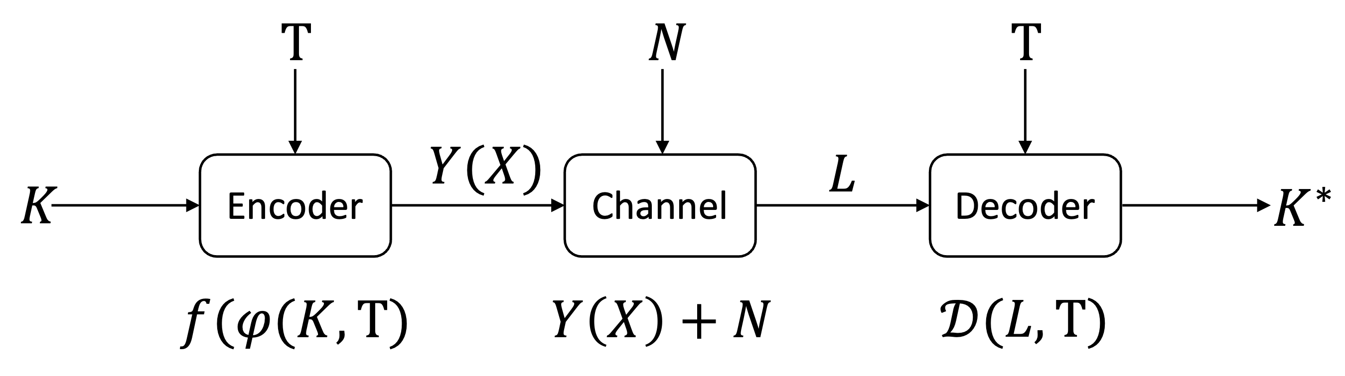
Figure 1. Side Channel Modeled as A Communication Channel

From information theory, mutual information ($MI$) (Unterluggauer et al., 2018; Standaert et al., 2009) is commonly used to measure the amount of information related to secret $X$ that is contained in the leakage trace $L$. Since $f(\cdot)$ is a deterministic function of $X$, as derived in (de Chérisey et al., 2019), we have

$$MI(L;X|\text{T})=MI(L;Y(X)|\text{T})=\mathbb{E}[MI(L;Y(X)|\text{T}=t)]$$

(2) $$\qquad\qquad\qquad\qquad\qquad\quad\ \ \ =H(Y(X))-H(Y(X)|L)~{}~{},$$

where $\mathbb{E}[\cdot]$ is the expectation operator, $H(Y(X))$ is the entropy of $Y(X)$ and $H(Y(X)|L)$ is the conditional entropy of $Y(X)$ based on $L$. The maximum mutual information leaked through a side-channel is typically called channel capacity (Cover and Thomas, 2006), which is expressed as:

(3) $$C=\max MI(L;Y(X)|\text{T})=\max MI(L;Y(X))~{}~{}.$$

Note here $C$ is measured by single trace. When $I_{q}$ traces are recorded, the channel capacity becomes $I_{q}\cdot{C}$ (Chérisey et al., 2019; Cheng et al., 2022).

We note a few differences between SCAs model and communication model: In SCAs, the leakage trace is measured (received) by the attacker. However, rather than acting as the receiver, now the attacker in fact plays the role of the eavesdropper as in the communication model (Goel and Negi, 2008). Hence, the attackers can not influence the internal state $X$ in the target implementation (transmitter) through the communications between the transmitter and the attackers as in the communication model (this is obvious as now $X$ is the unknown target secret), and therefore can not optimize the channel capacity of the side-channel. Previous work in (Unterluggauer et al., 2018) also focused on the same problem, where the authors construct the side-channel’s channel capacity by modeling the side-channel as MIMO (multi-input multi-output) channels (Goldsmith et al., 2003). However, the modeling of the side-channel does not have to be limited to the linear model. On the contrary, A variety of non-linear models have also been proposed and fully studied, such as convolutional neural networks (Benadjila et al., 2020) and the quadratic model (Doget et al., 2011). In this paper, similarity to the work in (Heuser et al., 2014; Chérisey et al., 2019; de Chérisey et al., 2019), we use a general model to characterize the side-channel. We treat the side-channel as an additive noisy channel, as shown in Eq. (1). Hence the channel capacity of the side-channel is expressed by (Cover and Thomas, 2006):

(4) $$C=\frac{1}{2}\log\left(1+\text{SNR}\right)=\frac{1}{2}\log\left(1+\frac{\|Y(X)\|^{2}_{2}}{\mathbb{E}[\|N\|^{2}_{2}]}\right)~{}~{},$$

where $\|\cdot\|_{2}$ is the $\ell_{2}$ norm. We also note that Eq. (4) is applicable to all forms of leakage models, despite HW or HD models, the linear models, or any non-linear models, given the recorded side-channel leakage $Y(X)$.

2.2. Using Random Noise to Counter SCAs

As shown in Eq. (4), the channel capacity is decided by the SNR of the received leakage signals. Hence, mitigating the effectiveness of the SCAs is equivalent to reducing the SNR of the leakage signals. In communication system, one effective way to reduce the SNR is to inject random noise into the transmitted signal, which therefore decreases the SNR of the signal received by the eavesdropper, and leads to the degrading of the eavesdropper’s channel capacity. This technique is generally referred as jamming (Shafiee and Ulukus, 2005), and has also been proven to be effective in combating SCAs (Shamir, 2000; Güneysu and Moradi, 2011).

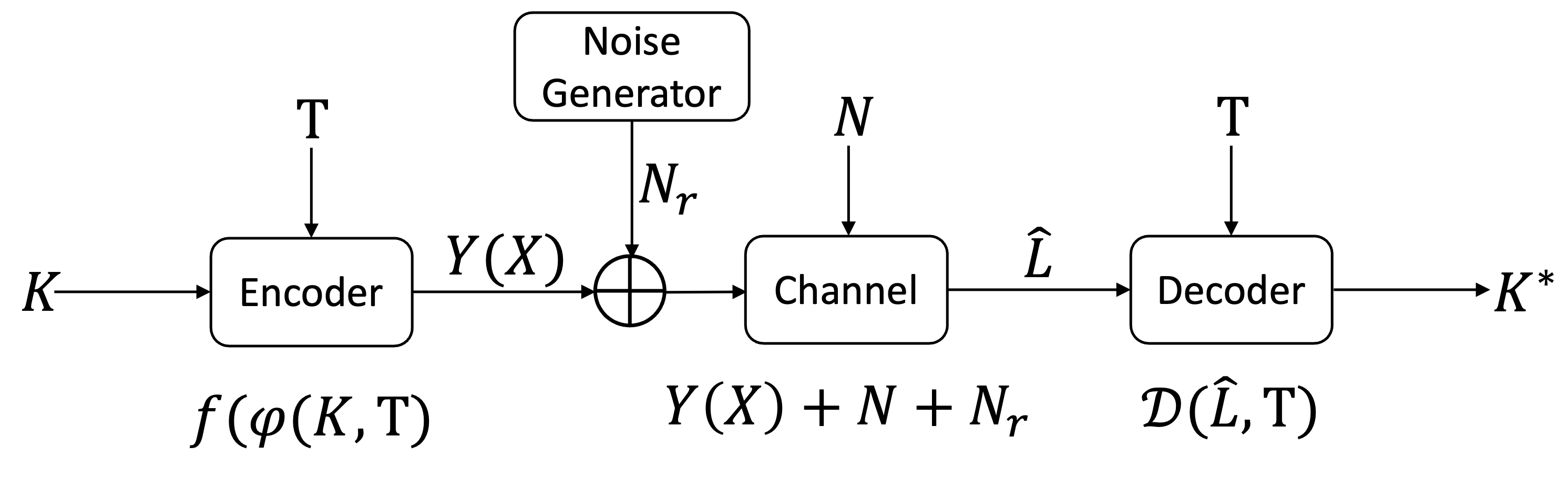
Figure 2. Side Channel Model with Random Noise Injection

Fig. 2 shows the side-channel model after applying the jamming. The random noise sequence is independently and randomly generated from the noise generator, which is then injected into the raw leakage trace $Y(X)$. As a result, the raw leakage trace and the random noise sequence are mixed together, which results in a “new” leakage trace that measured by attacker. Generally, the leakage traces superposed by the random noise can be expressed as:

(5) $$\widehat{L}=Y(X)+N+N_{r}~{}~{},$$

where $N_{r}$ is the i.i.d Gaussian noise vector with a distribution of $\mathcal{N}(0,\Sigma_{{r}})$. Now the capacity of the side-channel becomes:

(6) $$C=\frac{1}{2}\log\left(1+\frac{\|Y(X)\|^{2}_{2}}{\mathbb{E}[\|N\|^{2}_{2}]+\mathbb{E}[\|N_{r}\|^{2}_{2}]}\right)~{}~{}.$$

Compared to Eq. (4), the additional term $\mathbb{E}[\|N_{r}\|^{2}_{2}]$ decreases the SNR in Eq. (6) as well as the channel capacity $C$. As discussed in (de Chérisey et al., 2019; Chérisey et al., 2019), given a fixed $P_{s}$ which is the probability of success of an attack: $\mathbb{P}(K^{*}=K)$, the required minimum number of quires (number of traces) $I_{q}$ is inversely related to the SNR: $I^{\text{min}}_{q}\propto\frac{1}{\log(1+\text{SNR})}$. This means in order to achieve the same $P_{s}$, now attacker needs to record much more leakage traces, compared to the original SCAs.

Although the random noise generation method clearly works and is easily to be implemented, previous work also shows that this method leads to significant energy consumption: In (Das et al., 2017), the authors measured that in order to get a high enough resistance to side-channel attacks on AES, the current consumption is increased by a factor of four. This motivates us to design an energy efficient and also powerful noise generation scheme to counter SCAs.

3. Data Compression Technologies

Before introducing the design of our proposed scheme, we first discuss the compression of the leakage signal during the profiling and the attack phases. Typically, due to high sampling rates used, the recorded actual leakage trace $L_{o}$ has a very large number $m_{o}$ of samples where $m_{o}\gg m$ (note the recorded samples has already been composed of the same sized random part $N$ or even injected random noise $N_{r}$). However, it has been observed (such as in (Chari et al., 2003; Archambeau et al., 2006; Choudary and Kuhn, 2013)) that leakage traces are sparse, i.e. only very few leakage samples in the raw leakage traces contain useful information that is related to the internal state. This sparsity is caused by the fact that only a few logical components in the cryptographic system are depending on the secret in the predefined Input/Output (I/O) activities. Thus, in order to perform an effective attack, typically attacker has to compress the leakage traces in order extract the useful leakage information for attacking.

Based on how the samples are processed, typically the compression methods can be divided into two categories:

• Sample Selection: By selecting a subset from all recorded leakage samples, the number of samples is reduced. Samples are selected by using a variety of methods including Difference of Means (DoM) (Chari et al., 2003) (which includes 1ppc, 3ppc, 20ppc and allap), Sum of Squared Pairwise T-Differences (SOST) (Gierlichs et al., 2006), or Signal-to-Noise Ratio (SNR) (Mangard et al., 2008).

• Linear Combination: Using a linear transformation for projecting the raw leakage samples onto a low-dimensional subspace. Typically, this is done by using Principal Component Analysis (PCA) and Linear Discriminant Analysis (LDA) (Choudary and Kuhn, 2013; Archambeau et al., 2006; Standaert and Archambeau, 2008; Zhou et al., 2017).

Mathematically, independent from which methods is applied, the process of compression can be expressed as: $P{L_{o}}$, where $P\in\mathbb{R}^{m_{c}\times m_{o}}$ with $m_{c}\leq m$ is the compression matrix. The structure of the matrix $P$ corresponds to the category of compression methods:

Sample Selection

In this scenario, the compression matrix is also called the sampling matrix. Each row in $P$ has exact one ”1”, and the index of the ”1” in each corresponding column of $P$ stands for which sample in the recorded leakage signal is to be picked. (We can think of the sampling matrix as a permutation matrix with additional zero columns.).

Linear Combination

Any of the linear combination approaches uses a projection matrix, call it $\boldsymbol{U}$, to transform the raw leakage sample vector into a lower-dimensional vector. In PCA, $\boldsymbol{U}$ is composed of the first $m_{c}$ eigenvectors after applying the singular value decomposition (SVD) on the sample between groups matrix $B$ by selecting the top $m_{c}$ components; while in LDA, $\boldsymbol{U}$ is the first $m_{c}$ eigenvectors of $S^{-1}_{\text{pooled}}B$ where $S_{\text{pooled}}$ is the the common covariance of all groups (Choudary and Kuhn, 2013; Archambeau et al., 2006) (same as (Choudary and Kuhn, 2013), here we also assume $S_{\text{pooled}}$ is appropriately scaled hence the covariance between discriminants is the identity matrix). In the following, we treat $P=U$ for all the linear combination based methods.

However, no matter which compression method is chosen, the following observations for matrix $P$ are always held:

1. Right Inverse: We have $P\cdot P^{T}=I_{m_{c}}$ for all types of $P$, where $I_{m_{c}}\in\mathbb{R}^{m_{c}\times m_{c}}$ is an identity matrix.

2. Idempotent: Let $\hat{P}=P^{T}P$, we have $\hat{P}\cdot\hat{P}=\hat{P}$ for all types of $P$, where $\hat{P}\in\mathbb{R}^{m_{o}\times m_{o}}$ is a symmetric matrix.

These two observations will be used in the following to derive the energy efficient scheme.

4. Optimal Energy Efficient Artificial Noise Design

4.1. System Model of Artificial Noise Generation

In our designed model, the artificial noise sequence is also generated from the noise generator and injected into the raw leakage trace (same as in Fig. 2). The generated noise is denoted as $\widehat{N_{a}}$, which is defined by:

(7) $$\widehat{N_{a}}=\rho FN_{a}~{}~{},$$

where $\rho$ is the gain factor, and $N_{a}\in\mathbb{R}^{m_{o}}$ is an i.i.d Gaussian distributed noise vector with the distribution $\mathcal{N}(0,\Sigma_{{a}})$ where $\Sigma_{a}$ is a diagonal matrix with identical value $\sigma^{2}_{a}$ on the diagonal.

In Eq. (7), $N_{a}$ is the noise source of the noise generator, and $\rho$ is the gain on the amplitude of the generated impulsive noise. As we mentioned before, random noise generation is not energy efficient as it generates noises to corrupt all leakage samples. As introduced in Section 3, typically only a subset of leakage samples contain secret-dependent useful information. Hence, our designed noise sequence which aims at only corrupting those useful sample is in fact a impulsive noise sequence. Moreover, the artificial noise generator can directly apply the majority modules in the traditional impulsive noise generator (Mann et al., 2002), but only makes the change on the modeling of the inter-arrival times of the noise sequence: Different to the traditional impulsive noise generation, where the inter-arrival times of the impulsive noise is modeled as a Markov renewal process (MRP) (Mann et al., 2002; Levey and McLaughlin, 2002) and hence the inter-arrival time between two consecutive impulses is random (controlled by a Markov state-transition probability matrix), the inter-arrival times of our designed impulse noise is optimized given pre-defined energy overhead budget. More specifically, by explicitly control the generation of the noise, the impulsive noise sequence can superpose with the targeted information pattern contained in the leakage trace optimally, hence maximize the system security under SCAs.

Typically, the generation pattern could be represented by a state-transition probability matrix, and is stored and triggered in the control module in the noise generator. The transition matrix is expressed by $G=[\beta_{i,j}]$ with $1\leq i,j\leq n$, where $n$ is the total number of states in the impulsive noise generation, $\beta_{i,j}$ is the transition probability from state $s_{i}$ to $s_{j}$, and the state $s_{i}$ represents where the $i$-th impulse event should be occurred in the sequence given the first $i-1$ impulses is optimized. Hence $n$ equals the maximum number of the impulses that could be generated in a duration. As we mentioned that the generation of the impulsive noise is optimized in our design, we have $\beta_{i,j}=1$ only if $s_{i}$ matches with the first $i$ impulses in $s_{j}$ ($s_{i}=s_{j-1}$), and $\beta_{i,j}=0$ for the rest of the cases. Here $G$ is in fact a sparse matrix since majority of the elements in $G$ is 0.

Actually, the structure of the transition matrix can be mapped to a process of impulsive noise samples selection. This selection of the generation of the impulsive noises (which can also be viewed as a set of instructions to trigger the impulsive generation or not) is represented by the diagonal matrix $F\in\mathbb{R}^{m_{o}\times m_{o}}$, which injects the impulsive noises into a subset of samples of the raw leakage trace. Values on the diagonal can be ”0” or ”1”, and the positions of the“1”s in the diagonal decide where the noise samples will be generated and injected into the leakage trace, i.e., for which samples in the leakage trace we inject the impulsive noises.

In contrast to the indiscriminate random noise generation approach that described in Section 2, the artificial noise generation model can exploit the fact of the sparsity in leakage trace as shown in Section 3, and only generate a small number of noise samples at the relevant timing to inject into the raw leakage trace. This brings the basis for us to design more energy-efficient scheme to generate noise sequence. As we can notice, the key point work is to design an appropriated $F$ to achieve the optimal energy-efficiency, which will be discussed in the following.

4.2. Optimization Problem in Artificial Noise Generation

Assuming now the recorded leakage trace is perturbed by an artificial noise sequence $\widehat{N_{a}}$, and a data compression method $P$ is selected, then after the data compression, the recorded leakage trace can be expressed by:

(8) $$P\widehat{L_{o}}=Y_{P}(X)+N_{P}+P\rho F{N_{a}}~{}~{},$$

where $Y_{P}(X)$ is the deterministic part and $N_{P}=PN$ is the random part noise, after compression. Then the channel capacity becomes:

(9) $$C=\frac{1}{2}\log\left(1+\frac{\|Y_{P}(X)\|^{2}_{2}}{\rho^{2}\mathbb{E}[\|PF{N_{a}}\|^{2}_{2}]+\mathbb{E}[\|{N}_{P}\|^{2}_{2}]}\right)~{}~{},$$

From the system model in Fig. 2, the operations in the noise generator are independent to the encoder in where the internal state is stored. Hence, the generation of the designed artificial noise sequence is based on the entire internal state space in the target implementation, and not specifically to any single internal state $X$, since we like to maximize the utilization of the protection for a wide spectrum of attacking techniques. We therefore take the expectation on $\|Y_{P}(X)\|_{2}$ over all states, which results in a constant ${E}_{X}=\mathbb{E}[\|Y_{P}(X)\|^{2}_{2}]$. We can therefore re-define the target channel capacity of the side-channel as

(10) $$C_{s}=\frac{1}{2}\log\left(1+\frac{E_{X}}{\rho^{2}\mathbb{E}[\|PF{N_{a}}\|^{2}_{2}]+\mathbb{E}[\|{N}_{P}\|^{2}_{2}]}\right)~{}~{}.$$

As noted in  (Goel and Negi, 2008), in order to guarantee the confidentiality of a secret communication, the noise injected into the channel must be designed to maximally degrade the eavesdropper’s channel. More specifically, the objective in (Goel and Negi, 2008) is to generate an artificial noise that maximizes the lower bound on the secrecy capacity, which is defined as the difference in mutual information between the transmitter-receiver pair and the transmitter-eavesdropper pair: $\widetilde{C_{sec}}=MI_{TR}-MI_{TE}$ where $\widetilde{C_{sec}}$ is the lower bound on the secrecy capacity, $MI_{TR}$ and $MI_{TE}$ are the mutual information on the transmitter-receiver and the transmitter-eavesdropper pairs, respectively.

However, there is small difference when applying above condition to SCAs models. In SCAs, there is no receiver as in the communication model, and we therefore don’t have to consider the transmitter-receiver pair. As a result, we can treat the mutual information in the transmitter-receiver pair as a constant value (for example let $MI_{TR}=0$). Hence, from the view of secret communication, maximizing the secrecy capacity in side-channel attacks is equivalent to minimizing the channel capacity in the transmitter-attacker (eavesdropper) pair, which happens to be correspond to the side channel in our problems. Therefore, our objective is to construct the noise sequence $\widehat{N_{a}}$ that can minimize the channel capacity $C_{s}$ of the side channel constraint by a threshold $E_{A}$ that caps the energy consumption for the noise generation:

(11) $$\min_{\widehat{N_{a}}}C_{s}\qquad\text{s.t.}\ \mathbb{E}[\|\widehat{N_{a}}\|_{2}^{2}]\leq E_{A}~{}~{}.$$

Noticed in Eq. (7), $F$ is used to control the generation of the artificial impulsive noise. More specifically, the rank of $F$ decides how many impulsive noise samples will be generated, which also decides the total energy to be spent in the noise generation. Hence the objective problem in Eq. (11) can be translated into:

(12) $$\min_{F}C_{s},\qquad\text{s.t.}\ \text{Rank}(F)\leq R_{A}~{}~{},$$

where $\text{Rank}(\cdot)$ counts the rank of a given matrix, and $R_{A}$ is the constraint on the number of impulsive noises that can be generated by the noise generator: $R_{A}=\frac{m_{o}E_{A}}{\rho^{2}\text{Tr}(\mathbb{E}[{N_{a}}{N_{a}}^{T}])}$, which is proportional to the amount of energy required to generate the impulsive noises. Note typically we take floor operation on $R_{A}$ ($R_{A}=\lfloor R_{A}\rfloor$) for enforcing it to be an integer.

4.3. Solution with Optimal Energy Efficiency

Since the independent noise $\text{E}[\|{N}_{P}\|^{2}_{2}]$ is fixed once $P$ is chosen, we only need to focus on the artificial noise part. From the Eq. (10), we can further obtain

(13) $$\mathbb{E}[\|PF{N_{a}}\|^{2}_{2}]=\mathbb{E}[{N_{a}}^{T}F^{T}P^{T}PF{N_{a}}]=\mathbb{E}[{N_{a}}^{T}F^{T}\hat{P}F{N_{a}}]~{}~{},$$

Letting $\Delta=F^{T}\hat{P}F$, based on the matrix trace operation, we have

(14) $$\rho^{2}\mathbb{E}[\|PF{N}_{a}\|^{2}_{2}]=\rho^{2}\mathbb{E}[\text{Tr}({N_{a}}^{T}\Delta{N_{a}})]=\rho^{2}\text{Tr}(\mathbb{E}[\Delta{N_{a}}{N_{a}}^{T}])~{}~{},$$

where $\text{Tr}(\cdot)$ is the trace operation. Furthermore, we have

(15) $$\rho^{2}\text{Tr}(\mathbb{E}[\Delta{N_{a}}{N_{a}}^{T}])=\rho^{2}\sigma^{2}_{a}\sum^{m_{o}}_{i=1}F_{ii}\hat{p}_{ii}~{}~{},$$

where $\hat{p}_{ii}$ and $F_{ii}$ are the $i$-th element on $\hat{P}$’s and $F$’s diagonal, respectively. Due to the monotonicity of the logarithmic function, one can easily find that minimizing $C_{s}$ in Eq. (12) is equivalent to maximizing the energy spent in the noise generation (the Eq. (15)). Further, the maximization of Eq. (15) under the energy constraint is in fact a typical 0-1 integer programming problem (Nemhauser and Wolsey, 1988). Therefore the problem in Eq. (12) can be translated as:

(16) $$\qquad\qquad\max_{F}\rho^{2}\sigma^{2}_{a}\hat{P}^{T}_{d}F_{d}\quad\text{s.t.}\ AF_{d}\leq R_{A},\ F_{d}\in\{0,1\}^{m_{o}}~{}~{},$$

where $\hat{P}_{d}\in\mathbb{R}^{m_{o}}$ and $F_{d}$ are the column vectors of the main diagonal elements of $\hat{P}$ and $F$ respectively, and row vector $A=[1,\dots,1]\in\mathbb{Z}^{1\times m_{o}}$. In Eq. (16), it’s clear that both $\rho^{2}$ and $\sigma^{2}_{a}$ are non-negative values. Since $\hat{P}$ is a symmetric idempotent matrix, its diagonal elements always satisfy $\hat{p}_{ii}\in[0,1]$. Hence, the objective in Eq. (16) is monotonically increasing with the increasing of $|\Omega_{F}|$ which is the cardinality of $\Omega_{F}$, where $\Omega_{F}$ is the set of the indices of ”1”s in $F$’s diagonal. Furthermore, when $|\Omega_{F}|$ is fixed ($|\Omega_{F}|=R_{A}$), based on the branch and bound method (Nemhauser and Wolsey, 1988), the maximum is decided by those most significant $\hat{p}_{ii}$ that are selected by $\Omega_{F}$.

More specifically, let’s first define $\Omega_{\hat{P}}$ as a set of the indices of $\hat{P}$’s diagonal elements, sorted in a decreasing order by $\hat{p}_{ii}$’s value. This means $\Omega_{\hat{P}}[1]$ is the index of the largest element in $\hat{P}$’s diagonal and $\Omega_{\hat{P}}[m_{o}]$ is the index of the smallest one. Moreover, $\Omega_{\hat{P}}[1:k]$ represents a subset of $\Omega_{\hat{P}}$ where only the first $k$ elements in $\Omega_{\hat{P}}$ are included. However, to an arbitrary set $\Omega_{\hat{P}}$, we are in fact only interested in those non-zero diagonal elements. Therefore, we further define a mapping $\Psi_{\hat{P}}(k)$ that outputs a set with the largest number of indices that corresponding to the non-zero diagonal element values, given an input subset $\Omega_{\hat{P}}[1:k]$, as:

(17) $$\Psi_{\hat{P}}(k)=\left\{\begin{array}[]{ll}\Omega_{\hat{P}}[1:k],\quad\text{if}\ \Omega_{\hat{P}}[k]>0~{}~{},\\ \Omega_{\hat{P}}[1:j],\quad\text{if}\ \Omega_{\hat{P}}[j]>0\ \&\ \Omega_{\hat{P}}[j+1]=0~{}~{},\\ \qquad\qquad\qquad\text{with}\ j<k~{}~{}.\end{array}\right.$$

Based on Eq. (17), we can obtain the optimum $F$ for the optimization problem in Eq. (16), which is

(18) $$F^{*}=\{F\ |\ \Omega_{F}=\Psi_{\hat{P}}(R_{A}),\ |\Omega_{F}|\leq R_{A}\}~{}~{}.$$

Note when $P$ is a sampling matrix, $\hat{p}_{ii}$ is either 0 or 1. Hence the order of the indices of the ”1”s in $\Omega_{\hat{P}}$ is randomly generated. Here one can easily find the main result in (Jin et al., 2022) (Eq. (24) in (Jin et al., 2022)) is in fact just a special case of Eq. (18) in our work.

Eq. (18) gives a solution to the design of an optimal energy-efficient artificial noise sequence under a given energy constraint $R_{A}$ and compression method $P$. However, in practice, normally there would be no prior information about which signal processing technique (the $P$) that attackers will use. For example, the system may choose 20ppc to construct the artificial noise during the design phase, but the attacker may prefer to use 3ppc. We will discuss how to apply our theoretical result into practical usage in next section.

5. A Practical Design of the Noise Generator

Following the optimal solution derived in Sec. 4, we propose an algorithm to construct a more practical energy-efficient noise generation mechanism for the system. Generally speaking, our algorithm is based on the philosophy of majority voting: First, during the design phase, the system designer picks a set of candidate compression methods: $\{P_{i}\}^{\zeta}_{i=1}$ with $\zeta$ is the total number of the selected compression methods. Based on Eq. (18), the corresponding optimums $\{\Omega_{F^{*}_{i}}\}^{\zeta}_{i=1}$ and $\{F^{*}_{i}\}^{\zeta}_{i=1}$ are therefore obtained, under a given energy constraint $R_{A}$. Then for each coordinate $i\in\{1,2,\dots,m_{o}\}$, if $i$ is labelled by the majority ($\geq 50\%$) sets of $\{\Omega_{F^{*}_{i}}\}^{\zeta}_{i=1}$, $i$ is selected into the final set $\Omega_{F_{o}}$. The final selection matrix $F^{*}_{o}$ that will be used in noise generation in practice is hence defined as

(19) $$F^{*}_{o}=\{F_{o}\ |\ \Omega_{F_{o}}=\boldsymbol{\psi},\ |\Omega_{F_{o}}|\leq R_{A}\}~{}~{}.$$

More details of our algorithm is illustrated in Algorithm 1 and Algorithm 2. Once we obtain the final design $F^{*}_{o}$, we can easily translate $F^{*}_{o}$ to the state-transition matrix $G^{*}$ that introduced in Sec. 4.1: For $i=1,2,\dots,m_{o}$, if the $i$-th element in $F^{*}$’s diagonal vector $F^{*}_{d}$ has:  $F^{*}_{d}[i]==1$, we set $s_{i}=F^{*}_{o}[1:i]$. Eventually, based on the states $s_{i}$ ($i=1,\dots,m_{o}$), transition matrix $G$ is reconstructed.

Algorithm 1 Majority Voting based Coordinate Selection

0:  $\{\Omega_{F^{*}_{i}}\}^{\zeta}_{i=1}$

  Initialize  $\ \boldsymbol{\psi}=\{1,2,\ldots,m_{o}\}$

  For $j=1,2,...,m_{o}$

   $\textbf{If}\ \textbf{Majority\textunderscore Voting}(j,\ \{\Omega_{F^{*}_{i}}\}^{\zeta}_{i=1})==0$

    $\boldsymbol{\psi}=\boldsymbol{\psi}\backslash j;$

  end

  $\boldsymbol{\psi}$

Algorithm 2 Majority_Voting

0:  $j,\ \{\Omega_{F^{*}_{i}}\}_{i=1}^{\zeta}$

  Initialize  $t=0,\ \rho=0$

  For $l=1,2,...,\zeta$

   $\textbf{If}\ j\in\Omega_{F^{*}_{l}}$

    $t=t+1;$

  end

  $\rho=\text{Round}(t/\zeta);$

  $\rho$

6. Analysis of the Noise Sequence Generation Scheme

6.1. Energy Efficiency

As we design noise generation in an energy efficient fashion, we need to be guided by a metric that informs us both of their effectiveness and the efficiency. The former measures in terms of the reduction of the successfulness of an attack, and the second measures in terms of the amount of energy that is consumed. We combine these two metrics together, and call it energy efficiency (EE), and use it to measure the reduction of the attack success rate per unit of energy spent in noise generation, which is expressed by:

(20) $${EE}=\frac{1-{Successful\textunderscore Key\textunderscore Recovery}}{Noise\textunderscore Energy}~{}~{},$$

where $Noise\textunderscore Energy$ is the total energy that spent in generating the noise sequences during an attack which is the sum of the energy of all noise sequences that are injected into the leakage traces that are collected by the attacker. $Noise\textunderscore Energy=\sum_{i=1}^{I}\text{E}[{|N_{r}^{(i)}|^{2}}]$ (or $\sum_{i=1}^{I}\text{E}[|\widehat{N_{a}}^{(i)}|^{2}$), where $N_{r}^{(i)}$ ($\widehat{N_{a}}^{(i)}$) is the random noise sequence (artificial noise sequence) that has been added to the $i$-th leakage trace and $I$ is the total number of the leakage traces. ${Successful\textunderscore Key\textunderscore Recovery}$ is a binary value, which indicates whether the attacker is able to recover the secret value during an attack. If the attacker recovers the key, the value of EE is zero; otherwise, the larger the EE is, the less energy has been spent to cause an unsuccessful attack, in other words, it is more energy efficient.

6.2. Security Analysis

As discussed in Sec. 2.2, with the injection of the random noise, the required number of leakage traces (quires) $I_{q}$ is highly increased, in order to achieve a target $P_{s}$ during the attack. More specifically, given the following inequality derived from (de Chérisey et al., 2019)

$$I_{q}\geq\frac{B+(P_{s}-1)\log(2^{B}-1)-H(P_{s})}{\frac{1}{2}\log(1+\text{SNR})}~{}~{},$$

as an example, if the SNR is decreased from 0.04 to 0.01, in order to obtain same $P_{s}$, the minimum number of traces $I^{\text{min}}_{q}$ which equals to the lower bound is increased by near a factor of 4, which means much more numbers of attack queries are required. This gives the basis for enhancing the security protection of the system under SCAs. Besides, we set the function: $\xi(P_{e})=B+(P_{s}-1)\log(2^{B}-1)-H(P_{s})$ for simplicity in the following.

Furthermore, same as in (de Chérisey et al., 2019), we also use the Kullback–Leibler divergence to analyze the relative entropy between any two distributions under additional noise injection, for getting a more tight bound on $P_{s}$: $\xi(P_{e})$. Suppose we have $\mathbb{P}_{({\boldsymbol{L}_{j}}|K_{i},\textbf{T})}$ with ($i=1,2$) follows a multivariate normal distribution: $\mathcal{N}(\boldsymbol{Y(X)}_{j},\sigma^{2}_{N}\boldsymbol{I})$, where $\boldsymbol{Y(X)}_{j}=f(\phi(K_{i},\textbf{T}))_{j}=(f(\phi(K_{i},{T}_{1}))_{j},\dots,f(\phi(K_{i},{T}_{I_{q}}))_{j})$, $f(\cdot)_{j}$ is the $j$-th point of the leakage function vector ($j=1\dots,m$), and $\boldsymbol{I}$ is an identity matrix. For any two keys $K_{1}$ and $K_{2}$, the Kullback-Leibler divergence on their distributions at $j$-th point is:

(21) $$\text{D}_{j}\left(\mathbb{P}_{({\boldsymbol{L}_{j}}|K_{1},\textbf{T})}||\mathbb{P}_{({\boldsymbol{L}_{j}}|K_{2},\textbf{T})}\right)=\frac{\|f(\phi(K_{1},\textbf{T}))_{j}-f(\phi(K_{2},\textbf{T}))_{j}\|^{2}_{2}}{2\sigma_{N}^{2}}~{}~{},$$

with $j=1,\dots,m$. We can easily find with the injection of noise sequence, $\sigma_{N}^{2}$ is increased to $\sigma^{2}_{N}+\sigma^{2}_{a}$. Hence the divergence is therefore decreasing, i.e., by setting $\sigma_{a}=\sigma_{N}$, the divergence value is reduced by a factor of 2. Based on the main result (inequality (5)) in (de Chérisey et al., 2019), here we have the following inequality holds:

$$\xi(P_{e})\leq\min_{j}-\mathbb{E}_{\textbf{T}}\mathbb{E}_{K_{1}}\log\mathbb{E}_{K_{2}}e^{-\text{D}_{j}}~{}~{},$$

where $\text{D}_{j}$ is defined in Eq. (21). It’s easily to find $\xi(P_{e})$ which is the LHS of the inequality, is strictly increasing with the increase of $P_{s}$. When T (also $I_{q}$) is fixed, the upper bound (the RHS) is decreasing with the injection of additional noise with $\sigma_{a}$. This decreased upper bound therefore downgrades the target $P_{s}$, which means, in another way, the effectiveness of defense is enhanced.

We further illustrate our proposed mechanism can provide same security as the random noise generation but in energy efficient manner. Let’s denote $\Omega_{m}$ as the set of the indices of the secret-dependent samples among the leakage trace under a given target implementation. $\Omega_{F_{o}}$ is the set of the indices obtained by our approach where $\Omega_{F_{o}}\subseteq\Omega_{m}$. It’s obviously that the SNR of the recorded leakage sample point is meaningful only if this point is in set $\Omega_{m}$ (means the Eq. (21) is valid under this case). Therefore the majority ($\geq 95\%$ in some cases) samples (they are in the complement of $\Omega_{m}$: $\Omega_{m}^{\complement}$) covered by the sequence under random noise generation are nothing but independent noise, which don’t contain any useful information. As a subset of $\Omega_{m}$, $\Omega_{F_{o}}$ only contains the useful leakage samples. When $\Omega_{F_{o}}=\Omega_{m}$, our mechanism obtains the same power as random noise generation with much less energy spent. Besides, if our mechanism gets same amount of energy budget as the random noise generation, our mechanism can provide much more stronger security than random noise generation by allocating the extra energy on the variance or gain of the impulsive noise samples in $\Omega_{F_{o}}$.

Besides, our proposed scheme is compatible to work together with the masking (Prouff and Rivain, 2013), for further enhancing the system’s security. As derived in (Ito et al., 2022), given the number of masking shares is $d$, $\xi(P_{e})$ is upper-bounded by

(22) $$\xi(P_{e})\leq I_{q}\log\left((2^{B}-1)(2\ln 2)^{d}\prod^{d}_{i=1}MI(L^{s}_{i};S_{i})+1\right)~{}~{},$$

where $S_{i}$ is the $i$-th share which results in the leakage trace $L^{s}_{i}$. Since each leakage $L^{s}_{i}$ is only dependent on $S_{i}$ and is independent to other shares, we can treat each $MI(L^{s}_{i};S_{i})$ as an independent channel and model it as the noisy channel as Eq. (1). By applying our noise generation mechanism on the leakage trace from each share, the mutual information on each share’s channel is further decreased: Let’s assume the MI value on each channel is decreased by a factor of $\triangle_{a}$ caused by the impulsive noise sequence with the variance of $\sigma_{a}$, then the value of the continued product among all MI is decreased by a factor of $\triangle^{d}_{a}$. Based on Eq. (22), $\xi(P_{e})$ is therefore largely decreased (so is the $P_{e}$), under fixed $I_{q}$.

6.3. Time Delay

From Sec. 4, it can be found that the effectiveness of the scheme depends on the alignment of the timing of impulsive noise and the target segment in the leakage trace. Ideally, the noise samples generated by Eq. (18) are expected to be exactly overlapped with the leakage samples in the same or close approximate timing window. However, in practice, due to the likely delay introduced by hardware circuit, the generated noise impulse sequence may not be perfectly aligned with the leakage trace, for example, the starting point of two sequences is different. This is also called asynchronization. Our result is derived under synchronized assumption, which can be viewed as the theoretical boundary in an ideal situation.

7. Experimental Results

We evaluate our proposed scheme on the Grizzly benchmark dataset described in (Grizzly, [n. d.]). Grizzly is based on leakage data collected from the data bus of the Atmel XMEGA 256 A3U, which is a widely used 8-bit micro-controller. Given the 8-bit nature of the system, there are 256 keys. For each key $K\in\{0,1,\ldots,255\}$, 3072 raw traces are recorded. Note since the target micro-controller only executes the load instruction on each key, we just treat T is fixed as constant during the operations. Hence now we have $X=K$. Typically, these recorded traces are divided into two sets: a profiling set and an attack set. Each raw trace has 2500 samples, and each sample represents the total current consumption in all CPU ground pins.

The compression methods that we used in the experiments include 3ppc, 20ppc, allap, LDA, and PCA, which are commonly used compression methods in side-channel attacks. We pick 3ppc, 20ppc, LDA, and PCA as the candidates of the compression methods used in Algorithm 1. In the Grizzly dataset, the number of samples obtained by these sample selection methods in each trace typically are: $18\sim 30$ for 3ppc, $75\sim 79$ for 20ppc, and $125$ for allap, respectively (Choudary and Kuhn, 2013). For PCA and LDA, we set the dimension after compression as 4 (now $m_{c}=4$) during the system design phase.

We compare our noise generation scheme to two other methods: Random Full Sequence and Random Partial Sequence. Random Full Sequence (Shamir, 2000) generates random noise at all time. As a result, all leakage samples are covered by random noise samples. Random Partial Sequence generates noises for adding onto only a randomly selected subset of the raw leakage samples. In order to fairly compare Random Partial Sequence to our scheme, we have both methods generate the same number $|\Omega_{F_{o}}|$ of noise samples. Hence the two scheme only differ in the selection of raw leakage samples to inject the noise into. In the following, we use the term PrArN to denote our proposed practical artificial noise generation scheme, the term SArN for the previous sample selection based noise generation scheme (Jin et al., 2022), and the terms RnF and RnP for Random Full Sequence and Random Partial Sequence, respectively.

7.1. Metrics and Settings

During the attack phase, for each key $k$, we independently run the attack 300 times by randomly picking the leakage traces from the attack set. We use the ${Successful\textunderscore Recovery\textunderscore Rate}$ ($SRR$) to measure the attack, which is the average success probability over all keys:

$${Successful\textunderscore Recovery\textunderscore Rate}=\frac{\sum_{K=0}^{2^{B}-1}{P}_{attack}(K)}{2^{B}}~{}~{},$$

where ${{P}_{attack}(K)}=\frac{{N_{hit}(K)}}{{N_{T}}}$. Here ${N_{T}}$ is the number of tests (in our case, $N_{T}$=300) and ${N_{hit}(k)}$ stands for how many times that key $k$ is successfully recovered during all ${N_{T}}$ tests. We defined the EE in Eq. (20). In our experiments, we use $EE_{avg}$ to measure the average energy efficiency of the noise generation for all keys, which is:

$$EE_{avg}=\frac{\sum_{K=0}^{2^{B}-1}\frac{\sum_{t=1}^{N_{T}}EE(K,t)}{N_{T}}}{2^{B}}~{}~{},$$

where $EE(K,t)$ is the $EE$ value for an attack on key $K$ in $t$-th test. To scale the result, we normalize the $Noise\textunderscore Energy$ in Eq. (20) by letting $Noise\textunderscore Energy=\frac{Noise\textunderscore Energy}{N_{T}N_{s}\sigma^{2}}$, where $\sigma$ is the variance of the generated noise sequence, and $N_{s}$ is the number of sample per trace. In order to fairly compare all noise generation methods, both $N_{r}$ and $N_{a}$ are generated from the same distribution. The parameters of the noise distribution is obtained from the raw leakage trace: We collect the raw leakage traces under $k=0$ and compute the mean and variance. We also use 1000 traces to compute the matrix $P$ for any given compression method.

7.2. Experimental Data and Analysis

In the following, we will use $I_{a}$ and $I_{p}$ to denote the number of profiling and attack traces for each key, respectively.

7.2.1. Results on Standard Template Attack

The attack algorithm used in the experiments is the linear model based Template Attack described in (Schindler et al., 2005; Jin and Bettati, 2018). In this attack, the leakage model is represented by a linear model (also called stochastic model in this context), and during profiling the leakage model is estimated from all or a subset of keys. Based on the estimated leakage model, the template, which typically is in form of Gaussian Model, for each key is built. In the attack phase, we select the candidate key with the maximum likelihood in matching. In our experiments, we use all keys (256 keys) for profiling the leakage model. As a baseline for key recovery, we also present the results of the original Template Attack (denoted by OA), which is the version without noise generated. Note as there is no noise generated for OA, EE has no meaning for OA.

Fig. 3 shows the recovery rates and EE values with different numbers of $I_{a}$ under attack compression methods: allp and LDA, respectively. Here $I_{p}$=500, and $I_{a}$ varies from 1 to 1000. $R_{A}$ is set to 150. We also compare the effect of the gain by presenting the results with the increased gain $\rho=2$ for PrArN and RnP (now $E_{A}^{{}^{\prime}}=4E_{A}$). From the figure, in general, it shows the proposed method PrArN outperforms all other noise generation methods for combating the side-channel attacks in both effectiveness (resistance) and efficiency (EE). When evaluating the effectiveness (Fig. 3(a) and Fig. 3(c)), we can find when $\rho=1$, even when $I_{a}$=1000, ArN can still decrease the recovery rate from $\geq 93\%$ (OA’s number) to $53.41\%$ (allap’s number) and $34.66\%$ (LDA’s number), which is significant. Besides, the effectiveness of PrArN is always better than RnP with same gain factor. Considering both RnP and PrArN generate the same number of noise samples, this is a good proof that the effectiveness of our proposed model relies on the fact that the generation of the noise samples is artificially designed and particularly target on the useful leakage samples. Hence, it’s also straightforward that RnP ’s EE values are always worse than PrArN’s, which is reflected in the experimental results in (Fig. 3(b) and Fig. 3(d)).

We also notice when an appropriate number of attack traces is used (such as $I_{a}\geq 500$), both PrArN ($\rho=1$) and RnF allow for almost the same recovery rates. If now we evaluate the efficiency by observing the EE values, we can clearly find that PrArN always displays better EE value. As a result, it proves that to achieve same or approximate level of security, our method has the benefits in spending much less energy compared to the RnF. When increasing $\rho$=2, PrArN further strongly enhances its power in defending SCAs. For example, when $I_{a}$=1000, PrArN can decrease the recovery rate to $30.52\%$ (allap) and $22.93\%$ (LDA), with average EE of 0.4803 (allap) and 0.5428 (LDA). As a baseline, the numbers of RnF with $\rho$=1 are: $52.86\%$ (allap) and $34.68\%$ (LDA) in $SRR$, and 0.0782 (allap) and 0.1083 (LDA) in $EE_{avg}$. Compared to RnF, the energy efficiency improvement conducted by PrArN is tremendous.

In Fig. 4, we present the results of the successful recovery rate and the average EE for different values of $R_{A}$, under LDA as the compression method chosen by the attacker. Here $I_{a}$ and $I_{p}$ are all fixed to 500. We also fix the gain $\rho$ =1 to control the overhead of the noise sequences. Note as OA has no noise generated, and RnF always covers the full size of leakage trace, $R_{A}$ has no impact on them. We just repeat the experiments and take average on all $R_{A}$.

In order to compare our model with the sample selection based method in (Jin et al., 2022), we also present the results of SArN under both 20ppc and allap, which are good examples to prove the effectiveness of our proposed method. As we mentioned before, the solution in (Jin et al., 2022) is in fact a special case of our solution. For SArN (20ppc), in Grizzly dataset, only when $A\geq 80$, it can get the full solution of $F$ (for allap this number is 125). When $A<80$, PrArN outperforms SArN (both 20ppc and allap) in both effectiveness and efficiency. This is because our designed approach, by aggregating the noise generation patterns from a variety of different compression methods, is much more effective in identifying the most significant useful leakage samples, by selecting them through the ordering of their importance (Eq. (18)). On the contrary, the sample selection based methods only relies on a single category of compression methods, which highly limits the chance of extracting the useful samples by exploiting the information in other domains. Furthermore, the sample selection based methods just randomly select a subset from the candidates (the set of indices of ”1”s), which would cause the problem that those most important samples can not be guaranteed to be selected by every time, especially when $R_{A}$ is small. This is also proved by the experimental results that when $R_{A}$ didn’t achieve the full solution, the performance of the sample selection based methods is much worse compared to PrArN. For example when $R_{A}=70$, the $SRR$ and $EE_{avg}$ for PrArN are $58.67\%$ and 2.4467, while for SArN (allap) those are $75.62\%$ and 1.4427. When the full solution is guaranteed, SArN can obtain the optimal result in effectiveness, same as PrArN. Note the comparison of the EE between PrArN and SArN is only meaningful when both of them are under the same valid number of $R_{A}$, as SArN will only generate $|\Omega_{\hat{P}}|$ impulsive noises when $R_{A}$ is larger than $|\Omega_{\hat{P}}|$.

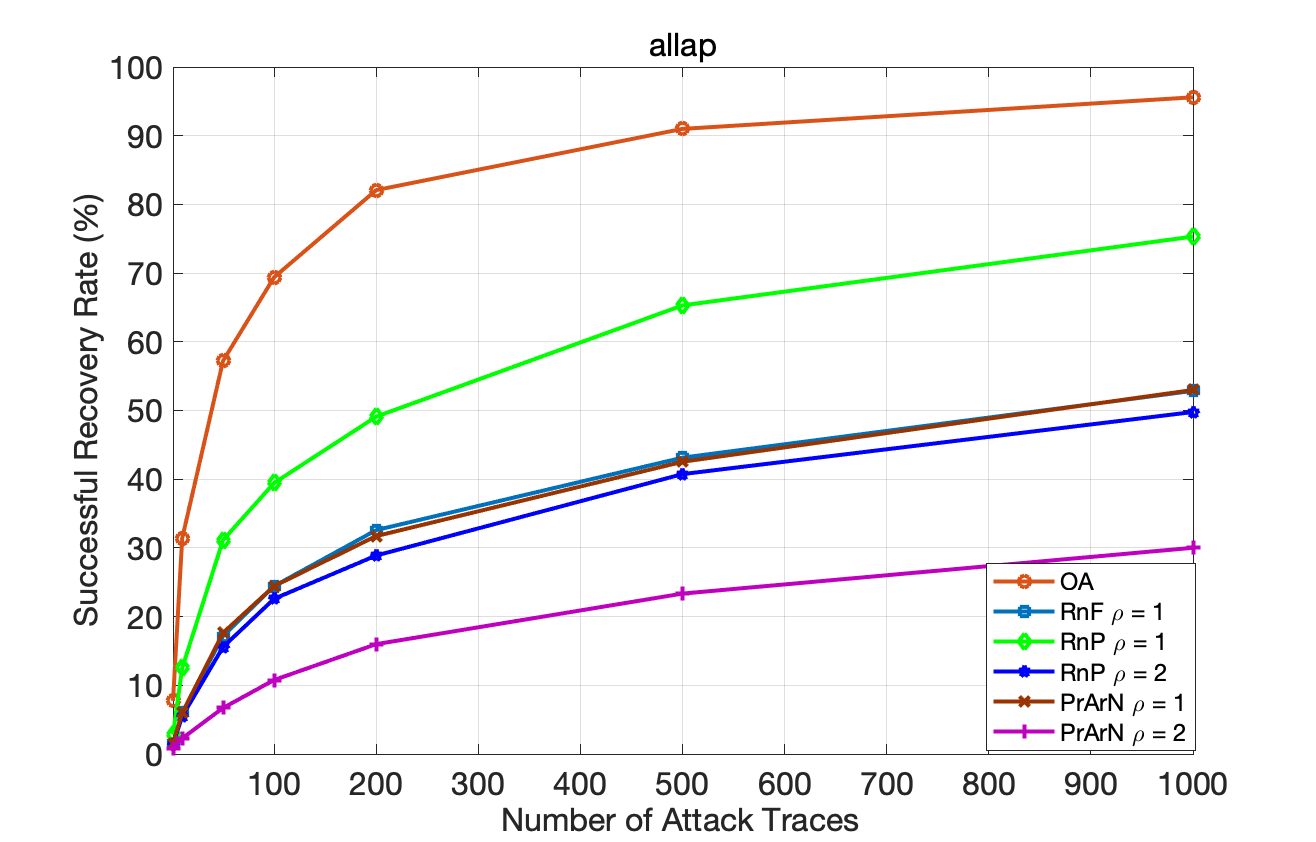
(a) SRR, allap

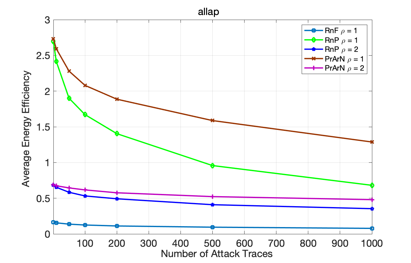
(b) $EE_{avg}$, allap

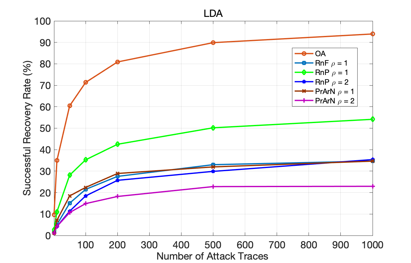
(c) SRR, LDA

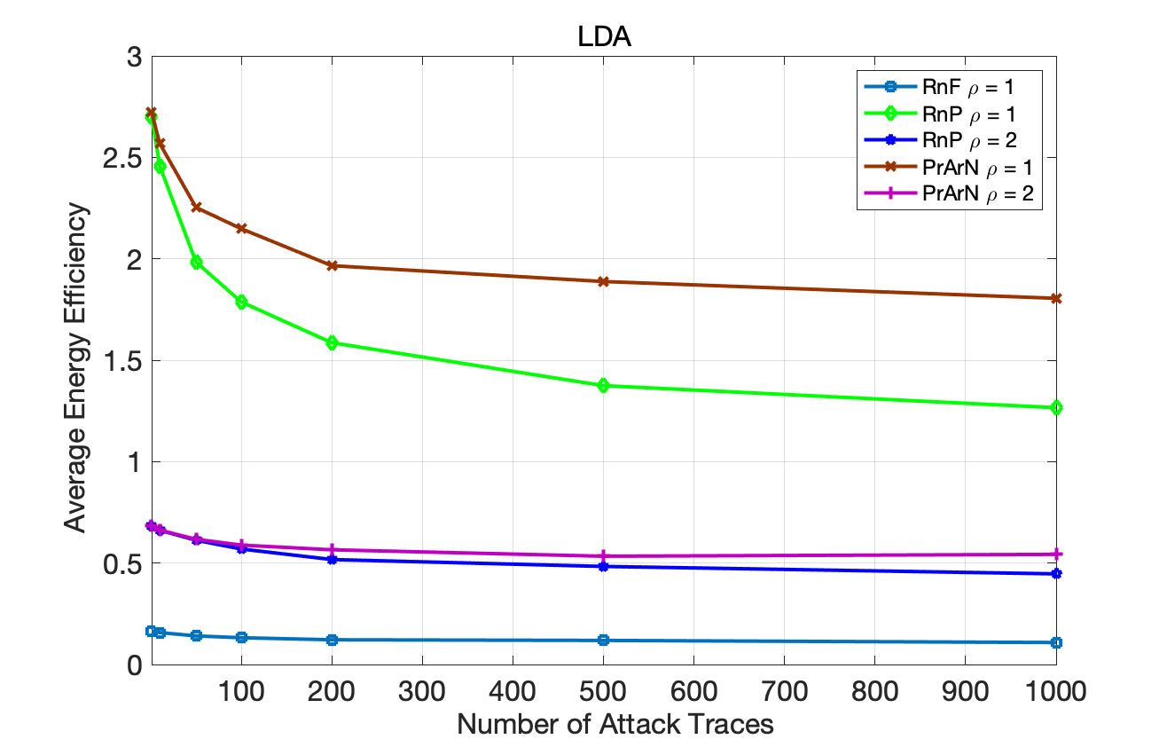
(d) $EE_{avg}$, LDA

Figure 3. Probability of Successful Recovery, and Average EE, versus Different Attack Traces $I_{a}$, under Compression Methods: allap and LDA for Attacker, respectively

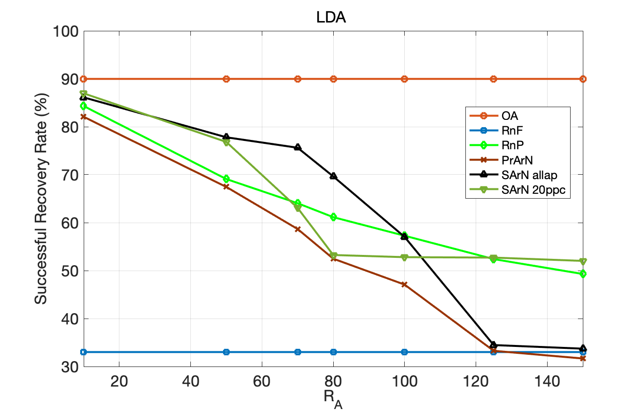
(a) SRR, LDA

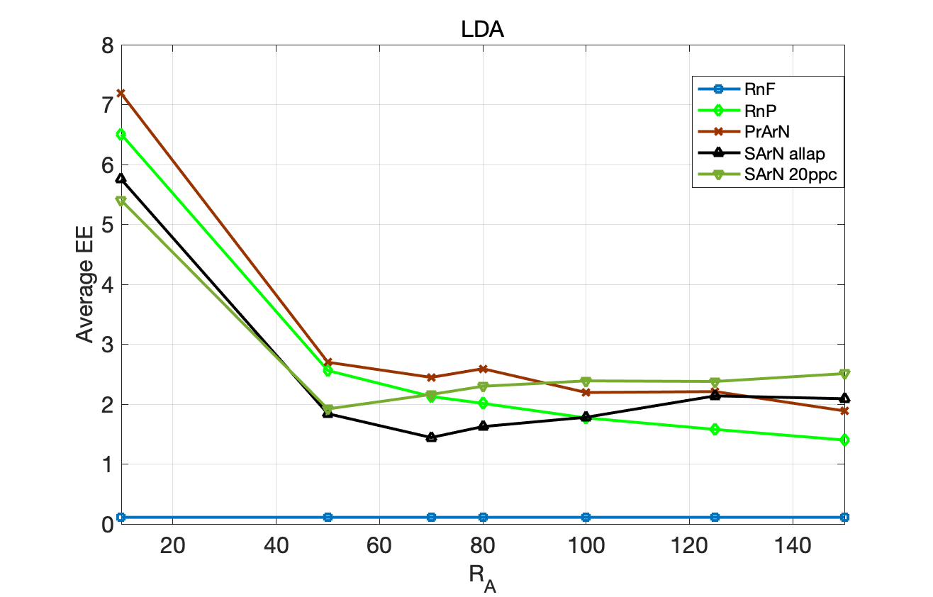
(b) $EE_{avg}$, LDA

Figure 4. Probability of Successful Recovery, and Average EE, versus Different $R_{A}$, under Compression Method: LDA for Attacker

7.2.2. Results on A DPA Style based Attack

Same as the work in (Choudary and Kuhn, 2018), we also use the same Grizzly data set to simulate a DPA (Differential Power Analysis) style (Whitnall and Oswald, 2015) based template attack on AES. Specifically, we treat each key $K$ as the actual output of $v=S(\text{T}\oplus K)$: We first generate a random key byte $K^{*}$ as the target key. Then for each leakage trace, we can compute the corresponding plaintext byte T to make $v=S(\text{T}\oplus K^{*})$ is the byte that actually be loaded and results in the leakage trace. During the attack phase, to each leakage trace $L_{i}$, the corresponding plaintext byte T is known. Then under this plaintext, for each candidate key byte $K$, we could compute the output of the Sbox operation: $S(\text{T}\oplus K)$ and obtain the corresponding output value $v$. Therefore, by combining multiple attack traces, the linear discriminant of each candidate key byte $K$ can be computed, as presented in (Choudary and Kuhn, 2018). Eventually, we guess the target key by picking the key byte which brings the maximum linear discriminant value. Note since now our target is just a single key byte, both the $SRR$ and $EE_{avg}$ are the results that over one key. Besides, in order to more fairly compare PrArN with SArN, here we make a modification on the original SArN: when $R_{A}>|\Omega_{\hat{P}}|$, now SArN will also generate $R_{A}$ impulsive noises, but these additional $R_{A}-|\Omega_{\hat{P}}|$ noises are randomly generated and added on the lekage trace.

Tab. 1 shows the successful recovery rate and the average EE for different methods $(P_{A}$) chosen by attacker: LDA and allap. We fixed $I_{p}=500$ and $I_{a}=100$, $R_{A}=125$, and $\rho=1$. SArN is under 20ppc. From the table, we can still easily find that our methods outperforms RnP and SArN in both $SRR$ and $EE_{avg}$, and RnF in $EE_{avg}$, under all two cases. For example, when $P_{A}$=allap, PrArN brings near $10\%$ decreasing on the recovery rate compared with SArN. Compared to RnF, PrArN obtains almost same recovery rate but with near 20 times gain in energy efficiency. Moreover, even now $R_{A}=125$, the original SArN (20ppc) can only generate a smaller number of impulsive noises. Even now we make up the differences on the number of noises, as SArN has no knowledge about other useful sample points that are not belonging to the set $|\Omega_{\hat{P}}|$, hence only random noises are generated, which is far less effective to resistant the SCAs. This also shows the limitation of SArN, and also a good proof of superior effectiveness of our proposal which makes the best effort to target on these useful information under a given energy budget in noise generation.

	OA	RnF		RnP		SArN		PrArN
	$SRR$ (%)	$SRR$ (%)	$EE_{avg}$	$SRR$ (%)	$EE_{avg}$	$SRR$ (%)	$EE_{avg}$	$SRR$ (%)	$EE_{avg}$
allap	100.00	58.83	0.0686	80.87	0.6792	68.13	1.0521	58.47	1.3885
LDA	100.00	45.27	0.1028	62.39	1.2489	56.72	1.4799	44.93	1.8842

Table 1. Probability of Successful Recovery, and Average EE, versus Different Compression Methods for Attacker

8. Conclusion

In this paper, we propose a practical approach for generating energy efficient artificial noise sequences to prevent SCAs. Our design of the artificial noise is the impulsive noise sequence, which exploits the sparsity among the raw leakage traces that only very few number of leakage samples contain the useful leakage information. Typically, the useful leakage information is extracted by the compression methods. Compared to previous work which only consider the sample selection based compression, our solution works for all categories of compression methods. Then by using channel capacity to measure the mutual information between the side-channel leakage and the secret, the optimal noise sequence design problem is translated to a side-channel’s channel capacity minimization problem, and we obtain the optimum under a given energy budget.

Furthermore, we also propose an approach to design a practical energy efficient noise generation mechanism by aggregating the optimal noise generation patterns under different compression methods. Compared to the previous noise generation which is only based on a specific compression method at a time, our approach enhances the power of protection and also the practicability.

References

- (1)
- Archambeau et al. (2006) Cédric Archambeau, Eric Peeters, François-Xavier Standaert, and Jean-Jacques Quisquater. 2006. Template Attacks in Principal Subspaces. In International Workshop on Cryptographic Hardware and Embedded Systems (CHES’06). Springer, 1–14.
- Benadjila et al. (2020) Ryad Benadjila, Emmanuel Prouff, Remi Strullu, Eleonora Cagli, and Cecile Dumas. 2020. Deep Learning for Side-Channel Analysis and Introduction to ASCAD Database. Journal of Cryptographic Engineering 10 (2020), 163–188.
- Brier et al. (2004) Eric Brier, Christophe Clavier, and Francis Olivier. 2004. Correlation Power Analysis with a Leakage Model. In International Workshop on Cryptographic Hardware and Embedded Systems (CHES’04). Springer, 16–29.
- Chari et al. (2003) S. Chari, J. R Rao, and P. Rohatgi. 2003. Template Attacks. In International Workshop on Cryptographic Hardware and Embedded Systems (CHES’03). Springer, 13–28.
- Cheng et al. (2022) Wei Cheng, Yi Liu, Sylvain Guilley, and Olivier Rioul. 2022. Attacking Masked Cryptographic Implementations: Information-Theoretic Bounds. In 2022 IEEE International Symposium on Information Theory (ISIT’22). IEEE, 654–659.
- Choudary and Kuhn (2013) Marios O. Choudary and Markus G. Kuhn. 2013. Efficient template attacks. In International Conference on Smart Card Research and Advanced Applications (CARDIS’13). Springer, 253–270.
- Choudary and Kuhn (2018) Marios O. Choudary and Markus G. Kuhn. 2018. Efficient, Portable Template Attacks. IEEE Transactions on Information Forensics and Security 13, 2 (2018), 490–501.
- Chérisey et al. (2019) Éloi de Chérisey, Sylvain Guilley, Olivier Rioul, and Pablo Piantanida. 2019. An Information-Theoretic Model for Side-Channel Attacks in Embedded Hardware. In 2019 IEEE International Symposium on Information Theory (ISIT’19). IEEE, 310–315.
- Cover and Thomas (2006) Thomas M. Cover and Joy A. Thomas. 2006. Elements of Information Theory. John Wiley & Sons, Inc.
- Das et al. (2019) Debayan Das, Anupam Golder, Josef Danial, Santosh Ghosh, Arijit Raychowdhury, and Shreyas Sen. 2019. X-DeepSCA: Cross-Device Deep Learning Side Channel Attack. In 2019 56th ACM/IEEE Design Automation Conference (DAC’19). ACM, 1–6.
- Das et al. (2017) Debayan Das, Shovan Maity, Saad Bin Nasir, Santosh Ghosh, Arijit Raychowdhury, and Shreyas Sen. 2017. High Efficiency Power Side-Channel Attack Immunity using Noise Injection in Attenuated Signature Domain. In 2017 IEEE International Symposium on Hardware Oriented Security and Trust (HOST’17). IEEE, 62–67.
- de Chérisey et al. (2019) Eloi de Chérisey, Sylvain Guilley, Olivier Rioul, and Pablo Piantanida. 2019. Best Information is Most Successful: Mutual Information and Success Rate in Side-Channel Analysis. In IACR Transactions on Cryptographic Hardware and Embedded Systems (CHES’19), Vol. 2019. Springer, 49–79.
- De Cnudde et al. (2016) Thomas De Cnudde, Oscar Reparaz, Begül Bilgin, Svetla Nikova, Ventzislav Nikov, and Vincent Rijmen. 2016. Masking AES with d+1 Shares in Hardware. In International Conference on Cryptographic Hardware and Embedded Systems (CHES’16). Springer, 194–212.
- Doget et al. (2011) Julien Doget, Emmanuel Prouff, Matthieu Rivain, and François-Xavier Standaert. 2011. Univariate Side Channel Attacks and Leakage Modeling. Journal of Cryptographic Engineering 1, 2 (2011), 123–144.
- Fang et al. (2022) Qiang Fang, Longyang Lin, Yao Zu Wong, Hui Zhang, and Massimo Alioto. 2022. Side-Channel Attack Counteraction via Machine Learning-Targeted Power Compensation for Post-Silicon HW Security Patching. In 2022 IEEE International Solid-State Circuits Conference (ISSCC’22), Vol. 65. IEEE, 1–3.
- Faruque et al. (2016) Al Faruque, Mohammad Abdullah, Sujit Rokka Chhetri, Arquimedes Canedo, and Jiang Wan. 2016. Acoustic Side-Channel Attacks on Additive Manufacturing Systems. In Proceedings of the 7th International Conference on Cyber-Physical Systems(ICCPS’16). IEEE, 1–10.
- Gandolfi et al. (2001) Karine Gandolfi, Christophe Mourtel, and Francis Olivier. 2001. Electromagnetic Analysis: Concrete Results. In International Workshop on Cryptographic Hardware and Embedded Systems (CHES’01). Springer, 251–261.
- Gierlichs et al. (2006) Benedikt Gierlichs, Kerstin Lemke-Rust, and Christof Paar. 2006. Templates vs. Stochastic Methods. In International Workshop on Cryptographic Hardware and Embedded Systems (CHES’06). Springer, 15–29.
- Goel and Negi (2008) Satashu Goel and Rohit Negi. 2008. Guaranteeing Secrecy using Artificial Noise. IEEE Transactions on Wireless Communications 7, 6 (2008), 2180–2189.
- Goldsmith et al. (2003) Andrea Goldsmith, Syed Ali Jafar, Nihar Jindal, and Sriram Vishwanath. 2003. Capacity Limits of MIMO Channels. IEEE Journal on Selected Areas in Communications 21, 5 (2003), 684–702.
- Grizzly ([n. d.]) Grizzly. [n. d.]. http://www.cl.cam.ac.uk/research/security/datasets/grizzly/. ([n. d.]).
- Güneysu and Moradi (2011) Tim Güneysu and Amir Moradi. 2011. Generic Side-Channel Countermeasures for Reconfigurable Devices. In International Workshop on Cryptographic Hardware and Embedded Systems (CHES’11). Springer, 33–48.
- Heuser et al. (2014) Annelie Heuser, Olivier Rioul, and Sylvain Guilley. 2014. Good is Not Good Enough: Deriving Optimal Distinguishers from Communication Theory. In International Workshop on Cryptographic Hardware and Embedded Systems (CHES’14). Springer, 55–74.
- Ito et al. (2022) Akira Ito, Rei Ueno, and Naofumi Homma. 2022. On the Success Rate of Side-Channel Attacks on Masked Implementations: Information-Theoretical Bounds and Their Practical Usage. In Proceedings of the 2022 ACM SIGSAC Conference on Computer and Communications Security (CCS’22). ACM, 1521–1535.
- Jin and Bettati (2018) Shan Jin and Riccardo Bettati. 2018. Adaptive Channel Estimation in Side Channel Attacks. In 2018 IEEE International Workshop on Information Forensics and Security (WIFS’18). IEEE, 1–7.
- Jin et al. (2022) Shan Jin, Minghua Xu, Riccardo Bettati, and Mihai Christodorescu. 2022. Optimal Energy Efficient Design of Artificial Noise to Prevent Side-Channel Attacks. In 2022 IEEE International Workshop on Information Forensics and Security (WIFS’22). 1–6.
- Kocher et al. (1999) Paul Kocher, Joshua Jaffe, and Benjamin Jun. 1999. Differential Power Analysis. In Advances in cryptology (CRYPTO’99). Springer, Springer, 789–789.
- Levey and McLaughlin (2002) David B. Levey and Stephen McLaughlin. 2002. The Statistical Nature of Impulse Noise Interarrival Times in Digital Subscriber Loop Systems. Signal Processing 82, 3 (2002), 329–351.
- Mangard et al. (2008) Stefan Mangard, Elisabeth Oswald, and Thomas Popp. 2008. Power Analysis Attacks: Revealing the Secrets of Smart Cards. Springer.
- Mann et al. (2002) Iain Mann, Stephen McLaughlin, Werner Henkel, Rob Kirkby, and Thomas Kessler. 2002. Impulse Generation With Appropriate Amplitude, Length, Inter-arrival, and Spectral Characteristics. IEEE Journal on Selected Areas in Communications 20, 5 (2002), 901–912.
- Nemhauser and Wolsey (1988) George L. Nemhauser and Laurence A. Wolsey. 1988. Integer and Combinatorial Optimization. Wiley-Interscience.
- Prouff and Rivain (2013) Emmanuel Prouff and Matthieu Rivain. 2013. Masking against Side-Channel Attacks: A Formal Security Proof. In 32nd Annual International Conference on the Theory and Applications of Cryptographic Techniques (Eurocrypt’13). Springer, 142–159.
- Schindler et al. (2005) Werner Schindler, Kerstin Lemke, and Christof Paar. 2005. A Stochastic Model for Differential Side Channel Cryptanalysis. In International Workshop on Cryptographic Hardware and Embedded Systems (CHES’05). Springer, 30–46.
- Shafiee and Ulukus (2005) Shabnam Shafiee and Sennur Ulukus. 2005. Capacity of Multiple Access Channels with Correlated Jamming. In 2005 IEEE Military Communications Conference’(MILCOM’05), Vol. 1. IEEE, 218–224.
- Shamir (2000) Adi Shamir. 2000. Protecting Smart Cards from Passive Power Analysis with Detached Power Supplies. In International Workshop on Cryptographic Hardware and Embedded Systems (CHES’00). Springer, 1–77.
- Standaert and Archambeau (2008) François-Xavier Standaert and Cédric Archambeau. 2008. Using Subspace-based Template Attacks to Compare and Combine Power and Electromagnetic Information Leakages. In International Workshop on Cryptographic Hardware and Embedded Systems (CHES’08). Springer, 411–425.
- Standaert et al. (2009) François-Xavier Standaert, Tal Malkin, and Moti Yung. 2009. A Unified Framework for the Analysis of Side-Channel Key Recovery Attacks. In 28th Annual International Conference on the Theory and Applications of Cryptographic Techniques (Eurocrypt’09). Springer, 443–461.
- Unterluggauer et al. (2018) Thomas Unterluggauer, Thomas Korak, Stefan Mangard, Robert Schilling, Luca Benini, Frank K. Gürkaynak, and Michael Muehlberghuber. 2018. Leakage Bounds for Gaussian Side Channels. In International Conference on Smart Card Research and Advanced Applications (CARDIS’18). Springer, 88–104.
- Whitnall and Oswald (2015) Carolyn Whitnall and Elisabeth Oswald. 2015. Robust Profiling for DPA-Style Attacks. In International Workshop on Cryptographic Hardware and Embedded Systems (CHES’15). Springer, 3–21.
- Zhou et al. (2017) Xinping Zhou, Carolyn Whitnall, Elisabeth Oswald, Degang Sun, and Zhu Wang. 2017. A Novel Use of Kernel Discriminant Analysis as a Higher-Order Side-Channel Distinguisher. In International Conference on Smart Card Research and Advanced Applications (CARDIS’17). Springer, 70–87.