DAFT: Distilling Adversarially Fine-tuned Models for Better OOD Generalization

Abstract

We consider the problem of OOD generalization, where the goal is to train a model that performs well on test distributions that are different from the training distribution. Deep learning models are known to be fragile to such shifts and can suffer large accuracy drops even for slightly different test distributions [1].

We propose a new method – DAFT – based on the intuition that adversarially robust combination of a large number of rich features should provide OOD robustness. Our method carefully distills the knowledge from a powerful teacher that learns several discriminative features using standard training while combining them using adversarial training. The standard adversarial training procedure is modified to produce teachers which can guide the student better. We evaluate DAFT on standard benchmarks in the DomainBed framework [2], and demonstrate that DAFT achieves significant improvements over the current state-of-the-art OOD generalization methods. DAFT consistently out-performs well-tuned ERM and distillation baselines by up to 6%, with more pronounced gains for smaller networks.

1 Introduction

Several recent works have shown that standard deep learning models trained with stochastic gradient descent (SGD) style methods can be fragile and might suffer a large drop in accuracy if the test data distribution (also known as target domain) is even slightly different compared to the training data distribution (also known as source domain) [1, 2]. However, in practice, it is quite challenging to obtain training data that exactly matches the test distribution. For example, due to privacy restrictions we may not be able to access the data of the actual customers of a web-application. Instead, training data is generated using crowd workers or by seeking volunteers who are willing to donate their data for training. This clearly leads to distribution shift between the training and test data.

Consequently, it is crucial to design models and training mechanisms that are robust to distribution shifts and can perform well on out-of-distribution (OOD) data. Even in settings where some amount of data can be collected from the final deployment setting, it should be relatively easier to adapt models with good OOD generalization. OOD problems have been studied in a variety of settings where different amounts of source/ target information might be available. We consider the OOD generalization setting which is one of the weakest settings, and requires only a labeled training dataset, without any information about the target dataset or even about the sources present in the training dataset. Note that this setting is slightly different and more challenging than the popular domain generalization setting which requires the identity of source domain for each training point. Even, in the domain generalization setting, several recent works [2, 3] show that a well-tuned ERM model is still competitive with SOTA methods.

We propose DAFT to mitigate the problem of OOD generalization; see Section 3 for the precise setting. DAFT is motivated by three key observations that we discuss below.

Recent works have demonstrated that adversarial training can learn more robust features compared to standard training [4, 5]. This in turn can lead to better performance in few shot and transfer learning settings where final few layers of the network are finetuned using target data [6]. However, on multiple standard OOD datasets where such finetuning is not feasible, we observe that vanilla adversarial training does not provide substantial improvements on larger datasets; see Table 1.

On the other hand, we observe that the representations learned by standard training are already capable of achieving good OOD performance, as is also observed in [7, 8, 9]. For example, on the iWildCam-WILDS dataset, if the model is trained with data from a source domain different from the target domain, the target domain accuracy is around 50%. However, if we train the model on the source domain and then finetune the final layer with a mix of data from the target and the source domain, the target domain accuracy jumps to 67.1%, demonstrating that features learned by standard training are indeed capable of achieving good accuracy on OOD data. Note that fine-tuning degrades source accuracy by only 2%, indicating that the features being used are indeed robust. We conduct further experiments on a binary version of the Coloured-FashionMNIST dataset [10] to establish this intuition that standard training does learn a few robust generalizable features, but they may be drowned out by several non-robust features – see Section 4.

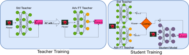
Figure 1: DAFT overview. We pre-train a teacher, followed by adversarial fine-tuning using $\mathcal{L}_{smooth}$ (2). We then distill a student from both standard and adversarial teachers. The Comp operator outputs $\hat{y}_{adv}$ if adversarial teacher’s prediction is correct, else it outputs $\hat{y}_{std}$.

Motivated by this observation, our first proposal is to pre-train the model using standard training and then, starting from this initialization, perform adversarial training of only the final linear layer. We call this adversarial finetuning. We observe OOD accuracy gains with this approach itself.

Our second intuition is that, OOD robustness can be improved significantly by diversifying the collection of standard features. Distillation [11] is known to help a student model access a larger set of “features" learned by the teacher model. Motivated by this intuition, we studied a method that combines PGD-AT[6] based adversarial finetuning with distillation, i.e., the teacher network is trained with ERM training followed by adversarial finetuning, and then distilled onto a student network. However, this method did not provide significant improvement over just using adversarial finetuning or distilling a standard trained teacher.

An explanation of this behavior is: while adversarial finetuning improves OOD robustness of the teacher, it also makes the logit predictions of all but the top class unstable. That is, while the “top" prediction value is stable due to adversarial finetuning loss, the remaining prediction values might change significantly with slight input perturbation. Hence, the predictions are possibly based on an unstable combination of features, leading to poor OOD performance. To alleviate this concern, we introduce a loss function – similar to one used by the TRADES algorithm [12] – that penalizes the distance between prediction values with and without adversarial perturbation. This leads to better teacher networks, since the incorrect teacher logits also provide useful information to the student.

Finally, to overcome the challenge of relatively poor accuracy of the adversarially finetuned teacher model on the training data distribution, we introduce a way to perform high quality distillation with respect to both the standard and adversarial finetuned teacher models.

Our contributions: In summary, we introduce a novel method – Distillation with Adversarially Finetuned Teacher (DAFT) – that uses the above algorithmic insights to design a robust technique for OOD generalization. DAFT trains a student model by distilling with a standard trained as well as an adversarially finetuned teacher model. Finetuning uses a smooth KL divergence based loss for all logits/prediction values. See Figure 1 for an overview of DAFT.

We conduct extensive experiments in the standard DomainBed framework [2] – using the prescribed methodology for evaluation, hyperparameter tuning – and compare DAFT against various baselines on the five OOD datasets in the testbed. Recall that even for stronger Domain Generalization setting, [2] showed that well-trained ERM is nearly SOTA. In contrast, we demonstrate that DAFT trained in the weaker OOD generalization setting, still consistently outperforms ERM (trained according to DomainBed approach) and other baselines. DAFT is particularly effective for smaller network architectures. For example, on DomainBed datasets, DAFT trained ResNet-50 models are on an average 4% more accurate than ERM as well as other baselines. In fact, DAFT+ResNet-50 models are more accurate than an ERM trained ResNet-152 as well; see Table 1. Finally, we conducted ablation studies to analyze the benefit of each of the algorithmic components introduced by DAFT. We observe that a combination of all the components of DAFT is critical towards achieving overall strong OOD performance.

Limitations: In general, different application areas/problems might lead to different forms of distribution shift between training and test distributions. Consequently, there may not be a single algorithm that is optimal under all distribution shifts. To address this, we perform experiments on multiple OOD datasets with different characteristics such as satellite images with temporal/geographical shift in TerraIncognita, and object images with varying sources in OfficeHome, VLCS, PACS and DomainNet datasets. In all of these settings, DAFT gives significant improvements over ERM. However, there may certainly be other forms of distribution shift, beyond those captured in the above datasets, where new ideas might be required to obtain superior performance.

2 Related Work

Generalization of a model to new domains has been studied in various contexts such as domain adaptation [13], domain generalization [2], OOD robustness/generalization [14, 1] and adversarial robustness [15, 6]. We now briefly review prior work from these areas.

Domain generalization and adaptation

In domain generalization, the training data is drawn from multiple domains or environments, each with a different distribution, and each training data point comes with its associated domain label. This fact is exploited by existing approaches by: a) learning domain invariant features[16, 17], b) matching feature representations across domains [18, 19], c) matching gradients across domains [20, 14], d) performing distributionally robust optimization across various domains  [21], e) augementing data with linearly interpolated samples from different domains [22, 23], f) learning common features across all the domains [24, 25], and g) learning causal mechanisms [26]. However, recent work [2] has shown that most of these methods perform no better than a well-tuned ERM over a larger model. Notable exceptions include results by [27] and a few others mentioned below. [27] proposes a training method to ensure flat minima which should lead to robustness. However, their technique assumes access to domain labels for creating batches and hence does not directly apply to our setting. It is also orthogonal to our work and can potentially be combined if batches are formed randomly. Concurrent and independent works in domain generalization setting either fine-tune with large pretrained models [7], or use the features from ERM trained models [8], or transfer features from large models to smaller models [28].

Unsupervised domain adaptation is a related problem setting [29, 30, 31, 32, 33], but these techniques rely on access to unlabelled target domain data and hence, do not apply to our setting.

OOD Robustness/Generalization

We study this setting, wherein no assumptions are made on the training or the test data domains. Due to a large diversity in domain shift mechanisms, several benchmarks have been introduced to evaluate OOD generalization including artificially induced domain shifts such as blurring, adding noise etc. [1], temporal, geographic and demographic shifts in natural settings [34, 35] etc. One approach to tackle this problem is to learn networks which side-step spurious correlations between the inputs and labels, using model pruning techniques [36]. We show that this method is less accurate than DAFT.

Recently, [37] demonstrated that larger models lead to better in-domain accuracy, which consequently leads to better OOD generalization. We exploit this intuition to try to transfer better features from larger models to smaller ones via distillation. In fact, using our method, significantly smaller architectures can outperform larger architectures in terms of OOD accuracy; see Table 1.

Adversarial Robustness

: Output of deep networks is known to be sensitive to small, carefully crafted perturbations of the input [15], and adversarial training (AT) [6] has been proposed to make models robust to such perturbations. A similar line of work, known as distributionally robust optimization trains networks to minimize the worst case performance on distributions in a small ball around the empirical distribution [38, 39, 40, 41]. Another line of work propose modifying the training objective of AT to ensure that all logits are similar for the clean and adversarial example [42, 12]. There have also been works which use adversarial training to promote adversarial distributional robustness in the learnt models [43, 44, 5, 45], bringing it closer to OOD robustness. However, the bounds in these works break down when the distribution shift is large, e.g. for datasets like PACS or VLCS. In this work, we demonstrate that, for OOD robustness, adversarial training of last layer tends to significantly outperform adversarial training of the entire network. While we use projected gradient descent (PGD) [6] and TRADES [12] methods to demonstrate the above claim due to their good empirical performance, we can in principle use any other AT method in their place.

Knowledge Distillation

: Knowledge distillation was introduced as a model compression technique which teaches a smaller model to mimic the outputs of a larger teacher [11]. Related works have also attempted at making students more robust to adversarial perturbations [46, 47] as well as using intermediate teacher representations to guide the student [48] but such methods do not consider OOD robustness of students. Furthermore, we demonstrate in Section 5 that DAFT outperforms vanilla distillation and distillation from an adversarially finetuned teacher (Table 1, Fig 2).

In summary, we find that most OOD works assume access to domain labels in one form or the other. In the OOD generalization setting where this assumption is dropped, ERM performs the best [2]. We show that DAFT consistently outperforms ERM, especially for smaller models.

3 Problem Definition

Problem setting: We are given a training dataset of labeled examples $\mathcal{D}_{S}=\left\{(x_{i},y_{i}):i\in[n]\right\}$, comprising of images from a single or multiple distributions. We do not assume access to domain labels. We assume access to a validation split from the test domain $\mathcal{T}$, which could be used for model selection in principle. In order to prevent the selection of hyperparameters that are tuned specifically to the target domain, we utilize the leave-one-domain-out validation method suggested by Gulrajani et al. [2]. This ensures that a common set of hyperparameters can be used for any combination of source domains in the dataset. While this was used for the purpose of evaluation and benchmarking, in practice, the target domain split alone could be used for model selection, which would lead to improvements over the reported results. We would like to emphasize that we do not have access to $\mathcal{T}$ during model training. While we do not assume any relationship between the training and the test data distributions, the datasets under consideration exhibit covariate shift, wherein the data marginal changes, while the conditional label distribution does not. Hence, we study this setting as it is more practically applicable.

Motivation: In several settings, there are privacy and proprietary reasons for not having access to the validation or target data (i.e., $\mathcal{V}$ and $\mathcal{T}$ respectively) during model training. However, once we train a model, we often have the ability to deploy/ evaluate the model for its accuracy on the validation domain $\mathcal{V}$, and in some cases, even on the target domain $\mathcal{T}$.

4 Method – DAFT

Data: Training data $\mathcal{D}_{S}=\left\{(x_{i},y_{i}):i\in[n]\right\}$, teacher model $(\theta,W)$, student model $(\mu,U)$, $\epsilon$, $\alpha$, Boolean: SingleDistill.

$\theta_{\textrm{std}}$, $W_{\textrm{std}}\leftarrow\textrm{Adam}\left(\min_{\theta,W}\sum_{i}\mathcal{L}_{\textrm{std}}(\theta,W,(x_{i},y_{i}))\right)$.

  /* Standard training of teacher model parameters $\theta$ and $W$. */ Using $\theta_{\textrm{std}}$, $W_{\textrm{std}}$ as initialization, optimize only $W$:
$W_{\textrm{adv}}\leftarrow\textrm{Adam}\left(\sum_{i}\mathcal{L}_{\textrm{adv},\epsilon,\theta}(W,(x_{i},y_{i}))+\alpha\cdot\mathcal{L}_{\textrm{smooth},\epsilon,\theta}(W,(x_{i},y_{i}))\right)$.

1  /* Smooth adversarial finetuning of final linear layer $W$. */ if SingleDistill then /* If SingleDistill is set to True then */

      DAFT-Single: ${\mu^{*},U^{*}}=\textrm{Adam}\left(\sum_{i}\mathcal{L}_{\textrm{distill}}(\mu,U,(x_{i},\tilde{y}_{i}))\right)$,
where $\tilde{y}_{i}=\frac{\exp\left(W_{\textrm{adv}}^{\top}f_{\theta_{\textrm{std}}}({x_{i}})/\tau\right)}{\sum_{\hat{y}}\exp\left(w_{{}_{\textrm{adv}},\hat{y}}^{\top}f_{\theta_{\textrm{std}}}({x_{i}})/\tau\right)}$

2        /* Train the student model using distillation loss $\mathcal{L}_{\textrm{distill}}$ defined in Eqn. (1), using only the adversarially finetuned teacher $(\theta_{\textrm{std}},W_{\textrm{adv}})$. */

3else

       DAFT: ${\mu^{*},U^{*}}=\textrm{Adam}\left(\sum_{i}\mathcal{L}_{\textrm{distill}}(\mu,U,(x_{i},\tilde{y}_{i}))\right)$,
where $\tilde{y}_{i}=\exp\left(W_{\textrm{adv}}^{\top}f_{\theta_{\textrm{std}}}({x_{i}})/\tau\right)/\sum_{\hat{y}}\exp\left(w_{{}_{\textrm{adv}},\hat{y}}^{\top}f_{\theta_{\textrm{std}}}({x_{i}})/\tau\right)$ if $(\theta_{\textrm{std}},W_{\textrm{adv}})$ correctly outputs $y_{i}$; else $\tilde{y}_{i}=\exp\left(W_{\textrm{std}}^{\top}f_{\theta_{\textrm{std}}}({x_{i}})/\tau\right)/\sum_{\hat{y}}\exp\left(w_{{}_{\textrm{adv}},\hat{y}}^{\top}f_{\theta_{\textrm{std}}}({x_{i}})/\tau\right)$.

4        /* Train the student model using distillation loss $\mathcal{L}_{\textrm{distill}}$ (1), where teacher logits are computed using adversarially finetuned teacher if it predicts correctly on this example; standard teacher otherwise. */

5 end if

Result: Trained model $(\mu^{*},U^{*})$.

Algorithm 1 DAFT: Distillation of Adversarially Fine-tuned Teacher

Motivation and high level description of algorithm: We begin by describing the key insights that led to our algorithm, and provide a high-level description. First key observation is that standard ERM trained models might already learn features which are good for domain generalization [9, 7, 8], but the final layer is not able to combine these features in a manner robust to domain shifts.

To further illustrate this point, we perform an experiment using a modification of a Fashion-MNIST subset with only two-class: shoe and top. We superimpose images onto coloured backgrounds, where the colour varies linearly between red $(255,0,0)$ and green$(0,255,0)$. Training images have a strong correlation between the background colour and label, i.e. color of tops images range from $(255,0,0)$ to $(123,132,0)$, while that of shoes images range between $(132,123,0)$ and $(0,255,0)$. In general, color can easily distinguish between the classes, but there is a small region between $(123,132,0)$ and $(132,123,0)$, where color cannot distinguish between the classes. During test time, there is no such correlation with colour i.e. the data is OOD w.r.t. the train data. For models trained on this data, we compute the correlation of each neuron at the output of the feature extractor with the shape and colour of the images. Note that color is a non-robust spurious feature while shape is a robust feature that is strongly correlated with the labels and is useful for prediction despite OOD shifts.

Now, an ERM trained model has an in-domain (ID) test accuracy of 99.9%, and OOD test accuracy of 60%. Furthermore, only 2 of the 32 features are highly correlated with the robust shape feature, while the rest are correlated with color. The final class output is dominated by the color features. In contrast, an adversarially trained model has a higher number of shape features (8 out of 32). But the in-domain accuracy is only 98.3%, and the OOD accuracy is 58%, lower than ERM. A probable reason is that even though adversarial training learns more shape-correlated robust features, but the average correlation with shape is much smaller (around $0.75$) than the similar correlation of features from standard trained model (around $0.8$). This is possibly because the shape features learned by adversarially trained models are more suited to the goal of adversarial robustness, while the features learned by standard ERM models are better correlated with the standard classification task. Hence, we introduce the method of adversarial fine-tuning of the last layer after standard ERM based pre-training. This encourages the model to give a lower prediction weight to color features, and higher weight to the robust shape features learned by the ERM model. With adversarial fine-tuning, a small ID accuracy drop 99.5% occurs, but the OOD accuracy jumps to 64%.

Next, motivated by the observation that distillation from larger models often helps in-domain performance, we trained our final model through distillation of a larger model which was itself trained using adversarial fine-tuning.

Surprisingly, vanilla distillation failed to transfer the superior performance of teacher model to the student model. We identify the main reason behind the failure of distillation in transfering the superior OOD performance of teacher to the student to be the following: while the Cross-Entropy loss on adversarial samples ensures that the logit corresponding to the correct class is “robust", it does not put any constraints on the remaining logits. Consequently, the remaining logits do not provide useful information for distillation. In order to tackle this, we add an additional KL divergence term to ensure that all the logits of the teacher model are smooth in the neighborhood of the given input, and are aligned to the logits of the clean image.

The final ingredient of our approach is to use two teacher models: the adversarially fine-tuned teacher on inputs where it predicts correctly and the standard trained model on the remaining inputs. We call the resulting algorithm Distillation of Adversarially Fine-Tuned teacher (DAFT). We now present each of the components in DAFT in more detail.

Adversarial fine-tuning: The first component is adversarial fine-tuning, where we first use standard training and then, using this as a pre-trained initialization, perform adversarial training of the final linear layer. The loss functions used in the standard pre-training and adversarial fine-tuning on a given data point $(x,y)$ are $\mathcal{L}_{\textrm{std}}(\theta,W,(x,y))$ and $\mathcal{L}_{\textrm{adv},\epsilon,\theta}(W,(x,y))$, respectively where,

where $f_{\theta}(x)$ denotes the penultimate layer representation of $x$ and $W$ is the final linear layer.
Note that while previous studies have shown that adversarial perturbations applied to the input of a network are amplified in the logit space, we tune the value of $\epsilon$ for getting the best performance on validation OOD data, which means that we can side-step this issue by having smaller perturbations. Further, we posit that while the perturbations in feature space will be large, the features which will be perturbed more are the non-robust features. We verify this empirically on the coloured-FashionMNIST dataset in the appendix, where we find that features corresponding to color get perturbed more than shape features. We would want our model to ignore such features. The training objective would ensure that this happens, leading to more robust models. We also conduct experiments with perturbing examples in the feature space and find that both these approaches yield similar empirical OOD performance (see Appendix).

Distillation from a larger teacher model: The second component is logit distillation – instead of training the model directly on the training dataset, we first train a larger teacher model using adversarial fine-tuning on the training dataset and then use logit distillation to train the desired model. Given an input $x$, temperature $\tau$ and teacher model $W$, the distillation loss for the student is given by:

$$\mathcal{L}_{\textrm{distill}}(\mu,U,(x,\tilde{y}))=KL(z,\tilde{y}),$$ (1)

$z=\exp\left(U^{\top}f_{\mu}(x)/\tau\right)/\sum_{\hat{y}}\exp\left(u_{\hat{y}}^{\top}f_{\mu}(x)/\tau\right)$, $\tilde{y}=\exp\left(W^{\top}f_{\theta}(x)/\tau\right)/\sum_{\hat{y}}\exp\left(w_{\hat{y}}^{\top}f_{\theta}(x)/\tau\right)$. Here $f_{\mu}(x)$ denotes the penultimate layer representation of $x$ and $U$ is the final linear layer corresponding to the student model, while $\theta$ and $W$ are the corresponding parameters of the teacher.

Smoothness of incorrect logits: The cross entropy loss function $\mathcal{L}_{\textrm{adv},\epsilon,\theta}$ in adversarial fine-tuning of teacher ensures that the logit corresponding to the correct class is large but does not explicitly consider logits corresponding to incorrect classes. However, logit distillation uses logits of the teacher model corresponding to all classes to train the student model. In order to ensure that logits of the teacher model corresponding to all classes are meaningful, we add an additional KL divergence term between logits of the given input and any other point in an $l_{2}$ norm constrained ball $B_{\epsilon}(x)$ around it.

$$\mathcal{L}_{\textrm{smooth},\epsilon,\theta}(W,(x,y))=\max_{\hat{x}\in B_{\epsilon}(x)}KL(z||\hat{z}),$$ (2)

where $z=\exp\left(W^{\top}f_{\theta}({x})\right)/\sum_{\hat{y}}\exp\left(w_{\hat{y}}^{\top}f_{\theta}({x})\right)$ and $\hat{z}=\exp\left(W^{\top}f_{\theta}(\hat{x})\right)/\sum_{\hat{y}}\exp\left(w_{\hat{y}}^{\top}f_{\theta}(\hat{x})\right)$. So the loss function we use in adversarial fine-tuning of the teacher is $\mathcal{L}_{\textrm{adv},\epsilon,\theta}+\alpha\cdot\mathcal{L}_{\textrm{smooth},\epsilon,\theta}$ for some $\alpha>0$. We note that this cumulative loss function is similar to that in TRADES with the key difference being that TRADES uses $\mathcal{L}_{\textrm{std},\theta}$ in addition to the KL divergence term, while we use $\mathcal{L}_{\textrm{adv},\epsilon,\theta}$ term. We use $l_{2}$ constrained perturbations, with the radius $\epsilon$ being a hyper-paremeter (whose value is mentioned in the appendix for various datasets).

Multi-distillation: Finally, as adversarial fine-tuning hurts in-domain accuracy and predicts incorrect labels for some in-domain training examples, we use different teachers for computing teacher logits on different examples. For those examples on which adversarially fine-tuned teacher predicts the correct label, we use the logits of adversarially fine-tuned teacher, while for those examples on which it predicts incorrectly, we use the logits of the standard trained teacher. More concretely, the loss function for DAFT is: $\min_{\mu,U}\sum_{i}\mathcal{L}_{\textrm{distill}}(\mu,U,(x_{i},\tilde{y}_{i}))$, where $\tilde{y}_{i}=\exp\left(W_{\textrm{adv}}^{\top}f_{\theta_{\textrm{std}}}({x_{i}})/\tau\right)/\sum_{\hat{y}}\exp\left(w_{{}_{\textrm{adv}},\hat{y}}^{\top}f_{\theta_{\textrm{std}}}({x_{i}})/\tau\right)$ if $(\theta_{\textrm{std}},W_{\textrm{adv}})$ correctly outputs $y_{i}$. Else, $\tilde{y}_{i}=\exp\left(W_{\textrm{std}}^{\top}f_{\theta_{\textrm{std}}}({x_{i}})/\tau\right)/\sum_{\hat{y}}\exp\left(w_{{}_{\textrm{adv}},\hat{y}}^{\top}f_{\theta_{\textrm{std}}}({x_{i}})/\tau\right)$. Here, $(\theta_{\textrm{std}},W_{\textrm{adv}})$ is the adversarially fine-tuned model, $(\theta_{\textrm{std}},W_{\textrm{std}})$ is the standard trained model. For ablation studies, we also present results for the vanilla version of DAFT, called DAFT-Single, where we only use the adversarilly finetuned teacher. The loss function for DAFT-Single is the same as above, except that $\tilde{y}_{i}=\exp\left(W_{\textrm{adv}}^{\top}f_{\theta_{\textrm{std}}}({x_{i}})/\tau\right)/\sum_{\hat{y}}\exp\left(w_{{}_{\textrm{adv}},\hat{y}}^{\top}f_{\theta_{\textrm{std}}}({x_{i}})/\tau\right)$ for all $i$. A pseudocode for the full algorithm including all these components is presented in Algorithm 1.

5 Experimental Results

Model Size	Method	PACS	VLCS	OfficeHome	DomainNet	TerraIncognita	Avg
ResNet-18	ERM	80.2$\pm$ 1.0	71.4$\pm$ 0.6	57.4$\pm$ 0.4	31.2$\pm$ 0.0	40.8$\pm$ 1.3	56.2
	AT	79.6$\pm$ 0.9	68.6$\pm$ 0.3	56.5$\pm$ 0.8	30.6$\pm$ 0.6	56.5$\pm$ 0.7	58.4
	TRADES	79.4$\pm$ 0.6	70.4$\pm$ 0.8	56.7$\pm$ 0.7	29.8$\pm$ 0.1	39.6$\pm$ 0.9	55.2
	Distillation	83.1$\pm$ 0.3	76.6$\pm$ 0.3	62.8$\pm$ 0.3	33.8$\pm$ 0.2	48.3$\pm$ 0.5	60.9
	DAFT	84.7$\pm$ 1.1	78.2$\pm$ 0.1	63.2$\pm$ 0.2	36.4$\pm$ 0.2	50.2$\pm$ 0.8	62.5
ResNet-34	ERM	83.2$\pm$ 0.8	73.5$\pm$ 1.0	60.8$\pm$ 0.6	32.5$\pm$ 0.0	41.0$\pm$ 0.7	58.2
	AT	82.2$\pm$ 1.0	72.9$\pm$ 0.5	60.5$\pm$ 0.5	30.7$\pm$ 0.3	40.6$\pm$ 0.4	57.4
	TRADES	82.5$\pm$ 0.6	72.2$\pm$ 0.7	60.7$\pm$ 0.8	31.4$\pm$ 0.3	41.3$\pm$ 0.2	57.6
	Distillation	84.0$\pm$ 1.7	76.0$\pm$ 0.7	66.3$\pm$ 0.1	36.7$\pm$ 0.1	48.5$\pm$ 0.9	62.3
	DAFT	87.4$\pm$ 0.3	79.1$\pm$ 0.9	67.2$\pm$ 0.5	38.5$\pm$ 0.3	51.4$\pm$ 1.1	64.7
ResNet-50	ERM	83.3$\pm$ 1.7	75.2$\pm$ 1.2	67.0$\pm$ 0.6	41.1$\pm$ 0.1	46.2$\pm$ 0.7	62.6
	AT	82.6$\pm$ 1.2	72.0$\pm$ 1.2	67.0$\pm$ 0.3	40.3$\pm$ 0.2	45.3$\pm$ 1.1	61.4
	TRADES	82.6$\pm$ 0.9	72.3$\pm$ 0.9	66.1$\pm$ 0.8	40.4$\pm$ 0.1	45.1$\pm$ 0.4	61.3
	Distillation	85.9$\pm$ 0.9	76.5$\pm$ 0.9	67.7$\pm$ 0.4	41.9$\pm$ 0.2	50.7$\pm$ 0.7	64.5
	DAFT	88.0$\pm$ 0.1	80.0$\pm$ 0.2	71.0$\pm$ 0.2	42.6$\pm$ 0.2	52.8$\pm$ 0.1	66.9
ResNet-101	ERM	85.0$\pm$ 0.0	76.9$\pm$ 0.4	67.6$\pm$ 0.5	42.6$\pm$ 0.1	49.5$\pm$ 0.0	64.3
	AT	72.6$\pm$ 0.1	75.9$\pm$ 0.4	67.5$\pm$ 0.4	42.3$\pm$ 0.1	47.9$\pm$ 0.1	61.2
	TRADES	83.7$\pm$ 0.5	76.3$\pm$ 0.4	68.0$\pm$ 0.3	42.2$\pm$ 0.1	49.5$\pm$ 0.8	63.9
	Distillation	86.9$\pm$ 0.7	77.1$\pm$ 0.4	69.1$\pm$ 0.2	43.2$\pm$ 0.1	50.3$\pm$ 0.3	65.3
	DAFT	88.8$\pm$ 0.5	79.1$\pm$ 0.5	72.2$\pm$ 0.8	43.7$\pm$ 0.5	54.1$\pm$ 0.9	67.6
ResNet-152	ERM	87.0$\pm$ 0.4	79.2$\pm$ 0.1	69.0$\pm$ 0.5	43.2$\pm$ 0.0	50.4$\pm$ 0.2	65.7
	AT	87.1$\pm$ 0.1	78.8$\pm$ 0.1	69.6$\pm$ 0.3	42.8$\pm$ 0.0	49.6$\pm$ 0.5	65.6
	TRADES	87.3$\pm$ 0.1	78.8$\pm$ 0.1	69.7$\pm$ 0.1	42.7$\pm$ 0.0	49.8$\pm$ 0.2	65.7
	Distillation	88.8$\pm$ 1.6	80.4$\pm$ 1.3	71.3$\pm$ 0.2	43.6$\pm$ 0.1	55.1$\pm$ 1.2	67.8
	DAFT	88.7$\pm$ 2.0	80.7$\pm$ 1.7	71.9$\pm$ 1.2	44.1$\pm$ 0.0	55.9$\pm$ 1.0	68.3

Table 1: OOD accuracy on various datasets with different ResNet (RN) architectures.

In this section, we detail our experimental setup, datasets, baselines and results.

5.1 Experimental Setup

Our experimental setup follows the approach and recommendations of [2]. For all our experiments, we train models of different sizes from the ResNet [49] family. We also perform augmentations including random cropping, flipping and colour jitter on the training data. Hyper-parameters for all the methods are tuned using the leave-one-domain-out approach descibed in [2]. See Appendix for additional details on hyperparameters. We use ImageNet pretrained models for comparisons on DomainBed. We report the mean and std deviation of the metrics across five random restarts.

Datasets

We report OOD accuracy results on 5 different datasets, and the average accuracy across them. We use all the datasets from the DomainBed [2] benchmark (i.e. PACS[24], VLCS[50], OfficeHome[51], DomainNet[52] and TerraIncognita[53]), whose details are in the appendix.

Baselines

We compare DAFT against the standard ERM method trained on training data $\mathcal{D}_{S}$. We also compare against AT which trains models using PGD for $l_{2}$-norm constrained input adversarial perturbations [6], as well as TRADES [12] which is a variant. This differs from adversarial fine-tuning introduced in Section 4 since it trains the entire network instead of just the final layer. Since DAFT uses larger models to train a smaller student network, we also compare it against the performance of distilling directly from an ERM trained teacher model. The teacher in all cases is ResNet-152.

5.2 Results

We compare the OOD accuracy of DAFT against baselines in Table 1. We notice that our method provides significant improvements over standard ERM across all datasets and model sizes For example, on OfficeHome, we show gains of almost 5% over ERM on all model sizes. We also note that smaller models trained with DAFT outperform ERM trained larger models; ResNet-34 trained with DAFT is close in performance to ResNet-152 on an average, while ResNet-50 can beat it.
We also notice that our method outperforms standard logit distillation on all benchmark datasets. This demonstrates that our method leverages the information provided by larger models in a more efficient manner. Furthermore, the KL-regularization of teachers in DAFT helps improve the transfer, as we demonstrate in the ablation experiments (sec 5.3).
We also observe that the method from [36] works only slightly better than ERM – on the OfficeHome dataset, the accuracies are 58.5%, 61.7%, 67.3%, 67.7% and 69.5% for ResNets 18-152 respectively. Their performance improvements are within the standard deviation of ERM trained models, and hence we do not compare against the method on the rest of DomainBed. We also notice that DAFT is able to outperform standard baselines by larger margins for datasets like TerraIncognita where the domains are significantly different from ImageNet. This means that features learnt from ImageNet pretraining would be less useful in this scenario. The better performance of DAFT on this dataset implies that it is able to transfer generalizable features better. Further, we perform experiments to verify the gains of DAFT without using ImageNet pre-trained networks on datasets from the WILDS [34] benchmark in the appendix.

5.3 Ablations

Model	Algorithm	PACS	VLCS	OfficeHome	Avg
ResNet-101	ERM	85.0$\pm$ 0.0	76.9$\pm$ 0.4	67.6$\pm$ 0.5	76.5
	AT	72.6$\pm$ 0.1	75.9$\pm$ 0.4	67.5$\pm$ 0.4	72.0
	AF	86.4$\pm$ 0.1	77.9$\pm$ 0.1	69.6$\pm$ 0.2	77.9
	TRADES	83.7$\pm$ 0.5	76.3$\pm$ 0.4	68.0$\pm$ 0.3	76.0
	AF+$\mathcal{L}_{smooth}$	86.5$\pm$ 0.1	77.6$\pm$ 0.3	69.5$\pm$ 0.3	77.9
ResNet-152	ERM	87.0$\pm$ 0.4	79.2$\pm$ 0.1	69.0$\pm$ 0.5	78.4
	AT	87.1$\pm$ 0.1	78.8$\pm$ 0.1	69.6$\pm$ 0.3	78.5
	AF	88.3$\pm$ 0.1	80.4$\pm$ 0.0	70.9$\pm$ 0.2	79.9
	TRADES	87.3$\pm$ 0.1	78.8$\pm$ 0.1	69.7$\pm$ 0.1	78.6
	AF+$\mathcal{L}_{smooth}$	88.4$\pm$ 0.4	80.4$\pm$ 0.0	70.9$\pm$ 0.3	79.9

Table 2: Effect of adversarial finetuning (AF): Accuracy achieved by ERM, adversarial training (AT) and adversarial finetuning (AF) for different architectures. Note that AF performs better than ERM, while AT is often worse than or similar to ERM due to poor in-domain accuracy of AT.

Does adversarial finetuning work?

To study the effect of our teacher training paradigms, we compare performance of various teacher models on the PACS, VLCS and OfficeHome dataset in Table 2. We show that it is much better to pre-train a model and finetune the final layer adversarially (AF), rather than training the full model adversarially (AT). Note that AT is competitive to ERM only on the OfficeHome dataset, since there is a high inter-domain similarity in three of the four domains of this dataset, and the images are also similar to ImageNet, on which the models were originally pretrained. This is consistent with the findings of [5].

Effect of $\mathcal{L}_{smooth}$ on distillation: To verify the effect of using teachers trained with $\mathcal{L}_{\textrm{smooth}}$, we present results on three datasets in Fig 2. For each split, we compute the average gain in OOD accuracy for the teacher (which is a ResNet-152) when trained with adversarial finetuning with ($\Delta_{\mathcal{L}_{\textrm{smooth}}}^{\textrm{Teach}}$) and without ($\Delta_{\textrm{AF}}^{\textrm{Teach}}$) $\mathcal{L}_{\textrm{smooth}}$. We then compare the gains over standard distillation observed in students distilled from these teachers ($\Delta_{\mathcal{L}_{\textrm{smooth}}}^{\textrm{Dist}}$ and $\Delta_{\textrm{AF}}^{\textrm{Dist}}$ respectively). Note that gain here refers to the difference in the OOD accuracy of the modified teacher (resp. distilled student of the modified teacher) model over a standard ERM (resp. distilled student of a standard teacher) model. We observe that students distilled from a teacher trained with $\mathcal{L}_{\textrm{smooth}}$ obtain similar or even better accuracy gains compared to those achieved by the teacher. In contrast, students of teachers trained without this term do not even consistently achieve similar accuracy gains as their teachers.

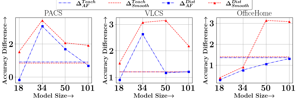
Figure 2: Importance of smoothness term $\mathcal{L}_{\textrm{smooth}}$ in teacher training for student performance: $(\Delta^{\textrm{Dist}}_{\textrm{Smooth}})$ and $(\Delta^{\textrm{Dist}}_{\textrm{AF}})$ denote accuracy increment for student models compared to std distillation, when distilled from a teacher with and without the smoothness term, respectively. Accuracy improvements for teacher over ERM are $\Delta^{\textrm{Teach}}_{\textrm{AF}}$ and $\Delta^{\textrm{Teach}}_{\textrm{Smooth}}$ when trained with and without smoothness term, respectively. Clearly, training the teacher with the smoothness term $\mathcal{L}_{\textrm{Smooth}}$ leads to accuracy improvements for students over and above improvements to the teacher accuracy.

Model	Algorithm	PACS	VLCS	OfficeHome	Avg
ResNet-18	DAFTSingle	82.39$\pm$ 0.3	77.72$\pm$ 0.3	62.73$\pm$ 0.7	74.44
	DAFT	84.65$\pm$ 1.1	78.16$\pm$ 0.1	63.20$\pm$ 0.2	75.18
ResNet-34	DAFTSingle	86.90$\pm$ 0.4	78.86$\pm$ 0.5	67.09$\pm$ 0.4	77.62
	DAFT	87.43$\pm$ 0.3	79.08$\pm$ 0.9	67.16$\pm$ 0.5	77.89
ResNet-50	DAFTSingle	87.66$\pm$ 0.2	78.73$\pm$ 0.5	69.34$\pm$ 0.4	78.58
	DAFT	87.86$\pm$ 0.2	79.64$\pm$ 0.4	70.85$\pm$ 0.3	79.45
ResNet-101	DAFTSingle	88.24$\pm$ 1.0	78.67$\pm$ 0.6	70.66$\pm$ 0.3	79.19
	DAFT	88.78$\pm$ 0.5	79.13$\pm$ 0.5	72.16$\pm$ 0.8	80.03

Table 3: DAFT vs DAFT-Single: Accuracies of DAFT and DAFT-Single show that using multiple teachers for distillation as in DAFT leads to significant improvements over using a single adversarially finetuned teacher as in DAFT-Single.

Effect of multiple teachers: We compare the OOD performance of student networks when trained with single or multiple teachers, i.e., DAFT-Single and DAFT respectively, in Table 3. We note that using multiple teachers consistently produce better students on average.

6 Conclusion

Summary: In this paper, we considered the problem of out of distribution (OOD) generalization, where we are given training examples from a source distribution and are required to output a model which will be evaluated on test examples sampled from a different target distribution. We first observed that the non-robustness of standard trained models on OOD data is primarily due to a non-robust combination of learned features in the final linear layer and that the features themselves are capable of obtaining high OOD accuracy. Inspired by this observation, we designed adversarial finetuning (AF) which first trains the model using standard training and then finetunes the final linear layer using adversarial training.

Motivated by the in-domain accuracy improvements obtained by distillation in prior works, we attempted to train a student model by distilling a teacher model that is trained by AF. However, we observed that standard distillation does not yield large improvements for AF trained teachers. We identified the reason for this to be the instability of logit values around the input and to address this, we incorporated an additional loss term in AF to encourage the logit values of teacher to be smooth. Finally, to tackle the suboptimal in-domain accuracy of AF trained teacher, we distilled both standard trained and AF trained teachers into the student giving our final algorithm DAFT.

On five benchmark datasets, with diverse kinds of distribution shifts, we showed that DAFT provides significantly higher OOD accuracy when compared to ERM as well as baselines like adversarial training. We also presented ablation studies showing the importance of various components of DAFT.

Limitations & Future work: While our experiments cover a diverse array of distribution shifts, and show that DAFT performs well, there may be other forms of distribution shift requiring further algorithmic ideas. Another avenue for future work is devising the optimal way of performing AF – in this work, we only consider finetuning the final linear layer but have not explored if this can be further improved by finetuning last few layers or other subsets of parameters. Finally, models that are fragile to OOD shifts and depend on spurious correlation can significantly amplify biases in data. So, further investigation of DAFT for mitigating biases in data is highly interesting.

Appendix A Experimental Setup

We use the same problem setting as Domainbed benchmark. We consider samples $(x_{1},y_{1}),...,(x_{n},y_{n})$ drawn from a training distribution $\mathcal{D}_{s}$. During test time, samples are drawn from a test distribution $\mathcal{T}$. Following Domainbed benchmark, we assume access to a pool of validation samples that are aggregated from multiple target domains. We cannot use these samples to train the model.
To further illustrate, let’s consider the example of the OfficeHome dataset. There are four sub-domains of the dataset - Art, Clipart, Photo and Product. For each of these sub-domains, the data is divided into a 80-20 split. Since there are four different sub-domains of this dataset, we essentially consider 4 different instances of the OOD generalization problem, wherein each problem considers one sub-domain as the test distribution, and the union of the remaining three as the train distribution. Both training and testing are always done on the 80% splits of the respective sub-domains. We then report the average test accuracy on all four instances of the problem for each method. We run this experiment 5 times across random restarts with the same hyper-parameters, and report the mean and standard deviations of the average test accuracy for each algorithm.
For hyperparameter selection, we use the leave one out setting mentioned in the Domainbed work [2] That is, given the four sub-domains of OfficeHome, we first sample $k$ hyper-parameter settings for an algorithm. For each of the $k$ hyper-parameter settings, we then train four models using the algorithm, leaving out one of the domains each time, and noting the accuracy of the model on the 20% split of the held out domain. The average of the four held-out accuracies is the validation accuracy of the hyper-parameter choice. We then choose the hyper-parameter setting which maximizes this validation accuracy.

A.1 Hyperparameters

We use the Adam optimizer for all our experiments, with a batch size of 64. We run ERM, adversarial training, and distillation for 10000 steps each, while fine-tuning is run for 5000 steps. We tune the following hyper-parameters for our methods and baselines -

• Learning Rate - Selected from the range $[10^{-6},10^{-3}]$

• Norm of adversarial perturbation $\epsilon$ - Selected from the range $[0.05,0.5]$

• Number of adversarial perturbation steps $k$ - An integer selected from the range $[3,7]$

• LR for PGD - Selected from the range $[10^{-3},10^{-1}]$

• Distillation temperature $\tau$ - An integer selected from the range $[2,8]$

• Weight $\alpha$ for $\mathcal{L}_{smooth}$ - Selected from the range $[10^{-6},10^{-2}]$

The hyperparameters were tuned using random search over the intervals, with $32$ configurations being considered for each algorithm.

A.2 Datasets

The data can be downloaded using the DomainBed repo

A.3 Hardware Setup

We conducted all experiments on a single A100 GPU. The experimental code was using the DomainBed framework, in PyTorch.

Appendix B Additional results

B.1 Statistical analysis of main results

We conduct paired t-tests of the results reported in table 1. In particular, we report the p-values of the the paired-t test between the results obtained by DAFT and Distillation in table 4. We boldface a value in table 1 if the corresponding p-value is less than 0.05.

Model	PACS	VLCS	OfficeHome	DomainNet	TerraIncognita
ResNet-18	0.132	0.011	0.020	0.003	0.016
ResNet-34	0.023	0.021	0.031	0.008	0.015
ResNet-50	0.011	0.018	0.010	0.015	0.001
ResNet-101	0.034	0.024	0.025	0.443	0.002
ResNet-152	0.117	0.449	0.212	0.077	0.315

Table 4: p-values of the paired t-test between the performance of DAFT and Distillation .

B.2 Results with the MobileNet architecture

We try out our method on mobilenet class of models (cite) and demonstrate that the observations for our method generalize form resnet models to mobilenet clas sof models as well. We perform experiments with the MobileNet [54] architecture where the teacher is a ResNet-152. The results are listed in table 5.

Model	Algorithm	PACS	VLCS	OfficeHome	TerraIncognita
MobileNetv3-Small	ERM	80.2	76.4	53.6	37.2
	Distillation	81.3	77.2	57.6	42.5
	DAFT	81.6	77.6	58.5	44.4
MobileNetv3-Large	ERM	85.9	79.8	63.1	47.8
	Distillation	86.9	81.1	66.5	51.1
	DAFT	87.5	82.1	67.2	53.8

Table 5: Comparison on the MobileNet family of architectures.

B.3 Results on WILDS benchmark

We perform experiments on the WILDS benchmark [34] with non-ImageNet pre-trained models to verify the efficacy of our approach in settings where pre-training on large datasets is not possible. We present results on iWildCams in Table 6. We notice that DAFT consistently gives gains over all the baselines.

Model	ERM	Dist	Adv	Trades	DAFT
RN-200	56.1 $\pm$ 0.4	56.7 $\pm$ 0.4	51.2 $\pm$ 1.2	53.0 $\pm$ 1.2	58.7 $\pm$ 0.6
RN-101	50.9 $\pm$ 0.3	55.8 $\pm$ 1.5	47.6 $\pm$ 1.0	50.2 $\pm$ 0.8	58.1 $\pm$ 0.4
RN-50	49.1 $\pm$ 0.5	55.4 $\pm$ 1.1	45.4 $\pm$ 1.1	47.9 $\pm$ 1.7	57.2 $\pm$ 0.5
RN-34	47.6 $\pm$ 0.9	52.5 $\pm$ 0.9	42.3 $\pm$ 1.7	45.5 $\pm$ 1.6	55.2 $\pm$ 1.5
RN-18	44.9 $\pm$ 0.6	50.7 $\pm$ 1.3	41.2 $\pm$ 1.8	42.7 $\pm$ 1.1	54.3 $\pm$ 1.3

Table 6: iWildCam dataset: OOD accuracy for different student architectures. RN refers to the ResNet architecture family. For all the considered RN models, DAFT is significantly more accurate than ERM and DIST, while vanilla ADV/TRADES training leads to worse OOD accuracy than ERM.

B.4 Detailed results on DomainBed

We present the domain-wise accuracies of DAFT for each of the datasets in DomainBed in tables 7-10.

Model Size	A	C	P	S	Avg
ResNet-18	82.5$\pm$ 2.0	82.7$\pm$ 1.8	93.1$\pm$ 2.1	80.8$\pm$ 0.1	84.8
ResNet-34	87.4$\pm$ 0.9	83.3$\pm$ 0.5	94.4$\pm$ 0.6	84.4$\pm$ 0.4	87.4
ResNet-50	88.2$\pm$ 1.4	84.3$\pm$ 1.1	94.6$\pm$ 0.8	84.9$\pm$ 0.5	88.0
ResNet-101	90.5$\pm$ 0.0	84.1$\pm$ 2.0	96.4$\pm$ 0.0	84.2$\pm$ 0.0	88.8
ResNet-152	88.1$\pm$ 1.0	84.3$\pm$ 1.3	95.8$\pm$ 0.9	86.3$\pm$ 1.1	88.6

Table 7: OOD accuracy of DAFT on various domains of PACS different ResNet (RN) architectures.

Model Size	C	L	S	V	Avg
ResNet-18	98.4$\pm$ 0.2	67.4$\pm$ 0.5	71.5$\pm$ 0.7	75.3$\pm$ 0.4	78.2
ResNet-34	98.7$\pm$ 0.4	66.5$\pm$ 1.7	73.3$\pm$ 1.4	77.9$\pm$ 0.6	79.1
ResNet-50	98.7$\pm$ 0.4	68.9$\pm$ 0.8	73.7$\pm$ 0.6	78.5$\pm$ 0.4	80.0
ResNet-101	98.6$\pm$ 0.0	69.6$\pm$ 1.8	73.6$\pm$ 0.1	74.6$\pm$ 0.1	79.1
ResNet-152	98.4$\pm$ 0.5	69.9$\pm$ 1.3	73.6$\pm$ 0.2	80.7$\pm$ 2.2	80.7

Table 8: OOD accuracy of DAFT on various domains of VLCS different ResNet (RN) architectures.

Model Size	Art	Clipart	Product	Real	Avg
ResNet-18	56.7$\pm$ 1.3	51.7$\pm$ 0.2	69.9$\pm$ 0.4	74.5$\pm$ 0.3	63.2
ResNet-34	61.1$\pm$ 1.3	56.0$\pm$ 1.1	74.6$\pm$ 0.3	77.3$\pm$ 0.3	67.2
ResNet-50	67.6$\pm$ 0.6	57.4$\pm$ 0.5	77.8$\pm$ 0.4	81.0$\pm$ 0.2	71.0
ResNet-101	68.9$\pm$ 0.0	59.5$\pm$ 0.1	78.4$\pm$ 0.3	81.9$\pm$ 0.1	72.2
ResNet-152	71.2$\pm$ 0.3	59.6$\pm$ 0.3	79.1$\pm$ 0.5	82.3$\pm$ 0.2	73.1

Table 9: OOD accuracy of DAFT on various domains of OfficeHome different ResNet (RN) architectures.

Model Size	L100	L38	L48	L46	Avg
ResNet-18	59.7$\pm$ 2.0	46.7$\pm$ 1.5	55.5$\pm$ 1.7	39.1$\pm$ 0.8	50.3
ResNet-34	61.1$\pm$ 2.3	48.0$\pm$ 1.2	58.0$\pm$ 0.6	38.7$\pm$ 1.2	51.5
ResNet-50	61.1$\pm$ 1.1	49.4$\pm$ 1.2	59.9$\pm$ 0.8	40.7$\pm$ 0.3	52.8
ResNet-101	62.2$\pm$ 1.4	50.1$\pm$ 1.7	60.7$\pm$ 0.7	43.2$\pm$ 0.8	54.0
ResNet-152	65.8$\pm$ 0.8	53.2$\pm$ 0.9	61.7$\pm$ 1.1	42.9$\pm$ 1.2	55.9

Table 10: OOD accuracy of DAFT on various domains of TerraIncognita different ResNet (RN) architectures.

Model Size	R	C	I	Q	P	S	Avg
ResNet-18	46.9$\pm$ 0.1	54.1$\pm$ 0.3	17.4$\pm$ 0.5	11.2$\pm$ 0.5	44.3$\pm$ 0.3	44.7$\pm$ 0.1	36.4
ResNet-34	50.8$\pm$ 1.8	55.8$\pm$ 0.4	19.4$\pm$ 0.4	12.8$\pm$ 0.2	46.5$\pm$ 0.2	45.8$\pm$ 1.2	38.5
ResNet-50	61.0$\pm$ 0.0	57.6$\pm$ 0.0	22.6$\pm$ 0.6	15.7$\pm$ 0.2	48.9$\pm$ 1.6	49.2$\pm$ 0.6	42.5
ResNet-101	63.8$\pm$ 0.3	59.7$\pm$ 0.2	23.5$\pm$ 0.3	16.4$\pm$ 0.3	48.5$\pm$ 0.2	49.8$\pm$ 0.1	43.6

Table 11: OOD accuracy of DAFT on various domains of DomainNet different ResNet (RN) architectures.

B.5 Results using Oracle strategy for hyper-parameter selection

Gulrajani et al. [2] note that using a hold-out validation set from the target domain can be a strategy for hyperparameter tuning in domain generalization. In table 12, we present the results obtained by using this on 4 datasets of DomainBed. We note that DAFT still out-performs other baselines in this case, and is considerably better than the results reported in Table-1 of the main paper.

Model Size	Method	PACS	VLCS	OfficeHome	TerraIncognita	DomainNet	Avg
ResNet-18	ERM	84.9$\pm$ 0.4	76.8$\pm$ 0.2	60.3$\pm$ 0.3	48.4$\pm$ 0.8	32.2$\pm$ 0.8	60.6
	AT	81.6$\pm$ 0.5	69.4$\pm$ 1.0	61.8$\pm$ 0.1	57.9$\pm$ 0.0	32.2$\pm$ 0.2	60.6
	TRADES	80.8$\pm$ 0.7	72.0$\pm$ 1.0	57.8$\pm$ 1.0	41.6$\pm$ 0.3	32.1$\pm$ 1.4	56.9
	Distillation	85.2$\pm$ 0.3	78.7$\pm$ 0.4	65.0$\pm$ 0.1	52.1$\pm$ 0.0	35.2$\pm$ 1.1	63.3
	DAFT	86.8$\pm$ 0.2	79.8$\pm$ 0.3	65.1$\pm$ 0.1	52.9$\pm$ 0.4	38.2$\pm$ 0.7	64.6
ResNet-34	ERM	88.2$\pm$ 0.4	79.6$\pm$ 0.4	64.7$\pm$ 0.1	50.9$\pm$ 1.0	33.6$\pm$ 0.5	63.4
	AT	84.2$\pm$ 0.2	75.3$\pm$ 0.2	65.2$\pm$ 0.3	43.1$\pm$ 0.8	32.5$\pm$ 1.2	60.1
	TRADES	84.0$\pm$ 1.3	73.5$\pm$ 0.1	62.9$\pm$ 0.4	43.7$\pm$ 0.8	33.3$\pm$ 1.1	59.5
	Distillation	88.7$\pm$ 0.2	79.9$\pm$ 0.1	68.8$\pm$ 0.2	54.2$\pm$ 0.4	38.9$\pm$ 0.1	66.1
	DAFT	89.3$\pm$ 0.1	81.3$\pm$ 0.3	68.7$\pm$ 0.1	54.8$\pm$ 0.3	39.7$\pm$ 1.1	66.8
ResNet-50	ERM	88.7$\pm$ 0.2	79.4$\pm$ 0.5	68.4$\pm$ 0.6	53.9$\pm$ 0.8	42.1$\pm$ 0.0	66.5
	AT	84.7$\pm$ 1.4	74.1$\pm$ 0.4	69.4$\pm$ 0.1	46.2$\pm$ 1.4	41.6$\pm$ 1.4	63.2
	TRADES	84.0$\pm$ 0.4	74.8$\pm$ 1.2	67.1$\pm$ 1.2	47.5$\pm$ 1.4	41.7$\pm$ 1.3	63.0
	Distillation	89.6$\pm$ 0.2	80.3$\pm$ 0.3	70.7$\pm$ 0.1	55.4$\pm$ 0.4	43.5$\pm$ 1.2	67.9
	DAFT	90.3$\pm$ 0.4	81.6$\pm$ 0.5	72.5$\pm$ 0.3	56.6$\pm$ 0.4	45.0$\pm$ 0.7	69.2
ResNet-101	ERM	88.1$\pm$ 0.0	79.1$\pm$ 0.0	68.7$\pm$ 0.0	52.1$\pm$ 0.0	44.2$\pm$ 1.0	66.4
	AT	73.6$\pm$ 0.7	76.4$\pm$ 1.4	71.8$\pm$ 0.1	49.3$\pm$ 0.8	44.4$\pm$ 0.9	63.1
	TRADES	84.9$\pm$ 1.3	78.8$\pm$ 0.3	69.4$\pm$ 0.9	51.4$\pm$ 0.6	44.2$\pm$ 1.2	65.7
	Distillation	90.8$\pm$ 0.2	80.5$\pm$ 0.1	71.8$\pm$ 0.1	55.6$\pm$ 0.4	45.1$\pm$ 1.0	68.8
	DAFT	91.5$\pm$ 0.0	82.2$\pm$ 0.1	73.0$\pm$ 0.2	56.5$\pm$ 0.2	45.5$\pm$ 0.7	69.8
ResNet-152	ERM	88.4$\pm$ 0.0	79.2$\pm$ 0.0	69.8$\pm$ 0.3	54.4$\pm$ 0.0	43.8$\pm$ 0.9	67.1
	AT	89.5$\pm$ 0.7	80.3$\pm$ 0.6	72.1$\pm$ 0.2	50.6$\pm$ 0.2	44.4$\pm$ 1.4	67.4
	TRADES	89.3$\pm$ 0.8	81.1$\pm$ 0.9	70.4$\pm$ 0.1	51.2$\pm$ 1.1	43.5$\pm$ 1.4	67.1
	Distillation	90.7$\pm$ 0.2	82.3$\pm$ 0.2	72.9$\pm$ 0.3	56.5$\pm$ 0.2	45.2$\pm$ 1.0	69.5
	DAFT	91.3$\pm$ 0.3	82.4$\pm$ 0.2	73.2$\pm$ 0.1	57.8$\pm$ 0.4	45.0$\pm$ 0.9	69.9

Table 12: OOD accuracy on DomainBed using the Oracle selection strategy for hyperparameter tuning.

Appendix C Verifying our Design Choices

C.1 Perturbing features instead of the input

We also experiment with a variant of adversarial fine-tuning where we perform perturbations in the feature space of the model rather than the input space. The comparison with adversarial finetuning on four datasets is reported in table 13. We notice that the difference in the performance obtained is not consistent across datasets or sizes. While the performance of finetuning in feature space is slightly more for ImageNet pre-trained models, we notice that the range over which $\epsilon$ needs to be fine-tuned is larger for this variant, and the obtained best $\epsilon$ differs quite a bit between different models. On the contrary, for input space perturbations, using the same $\epsilon$ across models does not degrade performance noticeably.

Input perturbations can potentially have an edge over feature space perturbations when the training data diversity is limited, leading to feature replication. In such a case, perturbing the relevant input pixels can perturb all the replicated features, while feature space perturbations need to individually perturb every replicated feature within the given perturbation budget. This is indeed the case when we do not use ImageNet pretraining, as seen in the last column of table 13.

Model Size	Method	PACS	VLCS	OfficeHome	FMoW
ResNet-101	AF	86.4	77.9	69.6	51.8
	AFLast	87.0	77.1	70.3	49.6
ResNet-152	AF	88.3	80.4	70.9	55.0
	AFLast	88.9	80.1	71.1	54.7

Table 13: Comparison between input perturbations and perturbations in the feature space.

C.2 Fine-tuning multiple layers

In table 14, we fine-tune the last three layers instead of just the final layer (AFMulti). We find that this leads to slightly improved performance on two datasets, and slightly degraded performance on one.

Model Size	Method	PACS	VLCS	OfficeHome
ResNet-101	AF	86.4	77.9	69.6
	AFMulti	87.1	77.7	70.5

Table 14: Effect of fine-tuning multiple layers.

C.3 Do adversarial perturbations lead to unstable logits?

In order to verify the effect of adversarial finetuning with and without the $\mathcal{L}_{smooth}$ loss, we compute the logits of an ERM trained model, an adversarially finetuned model and a KL-regularized finetuned model on the “Clipart" split of the OfficeHome dataset. The training and finetuning data for the adversarially fine-tuned models were the “Real", “Product" and “Painting" splits of the dataset, while the ERM trained model was trained on all datasets, i.e. it was also fine-tuned on the “Clipart" split. We find that the mean Spearman rank correlation of the logits from the KL-regularized model with the ERM trained model is higher (0.528) when compared to that of the adversarially finetuned model (0.505). In table 15, we list the average precision@k (k between 1-5) of the logits from adversarially finetuned models with respect to those of the ERM model (trained on source domain and source+target domains resp.). Here prec@k is defined as $|topk\_predictions(model)\cap topk\_predictions(ERMModel)|/k$. As we can see, $\mathcal{L}_{smooth}$ encourages the order of logits to be maintained (w.r.t. ERM model trained on source domain), while also being more similar to that of the ERM model trained on all domains, although its target accuracy is similar to the AF model.

Method	ERM Model	prec@1	prec@2	prec@3	prec@4	prec@5	MAP
AF with $\mathcal{L}_{smooth}$	Src+Tgt	62.5%	51.5%	48.9%	47.9%	47.5%	69.9%
AF	Src+Tgt	62.1%	49.4%	47.2%	46.9%	46.5%	67.4%
AF with $\mathcal{L}_{smooth}$	Src	94.1%	63.1%	53.2%	49.7%	48.8%	72.6%
AF	Src	94.1%	59.3%	50.1%	48.1%	48.0%	69.4%

Table 15: Comparison between teachers trained with and without $\mathcal{L}_{smooth}$. We show the overlap in the order of the predictions here, and note that the OOD predictions of smooth teacher are better aligned with the ERM teacher.

C.4 Additional results on Colored-FashionMNIST

In fig 3, we show examples of images from the FashionMNIST dataset, as well as the $l_{2}$-norm constrained adversarial perturbations. We choose the first three images of each label from the test set to perturb. We find that the perturbations mainly change the colour of the images. For each feature, we compute the relative average perturbation (RAP, i.e. $\mathbb{E}[\frac{|f_{i}(x+\delta)-f_{i}(x)|}{|f_{i}(x)|}]$, where $\delta$ is the adversarial perturbation, and $f_{i}$ denotes the $i^{th}$ feature) when the input is perturbed adversarially. We call this RAP-input. We also compute the relative average perturbation when the adversarial perturbations are in the feature space, denoted as RAP-feature. We notice that the maximum RAP-input for colour features is much more than that of shape features (11 v/s 0.4). This is expected since the adversarial perturbations only change the colour of the image. Hence, the model learns to weigh the colour features lesser while making predictions, since they change more while the label remains constant during adversarial fine-tuning. Further, we also notice that there is a high correlation (0.842) between RAP-input and RAP-feature. In fact, RAP-feature also follows a similar trend, with the maximum RAP-feature for shape features being 0.3, while the maximum RAP-feature for colour features is 13. This means that fine-tuning the last layer with either feature perturbations or input perturbations would lead the model to similar classification weights.

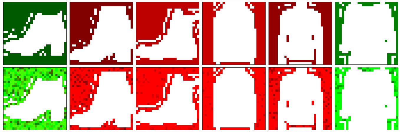
Figure 3: Sample images and their adversarially perturbed versions from Colored-FashionMNIST dataset. We notice that the color of the image is perturbed, while the shape remains constant.

References

- [1] Dan Hendrycks and Thomas G. Dietterich. Benchmarking neural network robustness to common corruptions and perturbations. CoRR, abs/1903.12261, 2019.
- [2] Ishaan Gulrajani and David Lopez-Paz. In search of lost domain generalization, 2020.
- [3] Ramakrishna Vedantam, David Lopez-Paz, and David J Schwab. An empirical investigation of domain generalization with empirical risk minimizers. In M. Ranzato, A. Beygelzimer, Y. Dauphin, P.S. Liang, and J. Wortman Vaughan, editors, Advances in Neural Information Processing Systems, volume 34, pages 28131–28143. Curran Associates, Inc., 2021.
- [4] Andrew Ilyas, Shibani Santurkar, Dimitris Tsipras, Logan Engstrom, Brandon Tran, and Aleksander Madry. Adversarial examples are not bugs, they are features. arXiv preprint arXiv:1905.02175, 2019.
- [5] Mingyang Yi, Lu Hou, Jiacheng Sun, Lifeng Shang, Xin Jiang, Qun Liu, and Zhi-Ming Ma. Improved ood generalization via adversarial training and pre-training. arXiv preprint arXiv:2105.11144, 2021.
- [6] Aleksander Madry, Aleksandar Makelov, Ludwig Schmidt, Dimitris Tsipras, and Adrian Vladu. Towards deep learning models resistant to adversarial attacks, 2019.
- [7] Ananya Kumar, Aditi Raghunathan, Robbie Jones, Tengyu Ma, and Percy Liang. Fine-tuning can distort pretrained features and underperform out-of-distribution. arXiv preprint arXiv:2202.10054, 2022.
- [8] Elan Rosenfeld, Pradeep Ravikumar, and Andrej Risteski. Domain-adjusted regression or: Erm may already learn features sufficient for out-of-distribution generalization. arXiv preprint arXiv:2202.06856, 2022.
- [9] Polina Kirichenko, Pavel Izmailov, and Andrew Gordon Wilson. Last layer re-training is sufficient for robustness to spurious correlations. arXiv preprint arXiv:2204.02937, 2022.
- [10] Han Xiao, Kashif Rasul, and Roland Vollgraf. Fashion-mnist: a novel image dataset for benchmarking machine learning algorithms, 2017.
- [11] Geoffrey Hinton, Oriol Vinyals, and Jeff Dean. Distilling the knowledge in a neural network, 2015.
- [12] Hongyang Zhang, Yaodong Yu, Jiantao Jiao, Eric P. Xing, Laurent El Ghaoui, and Michael I. Jordan. Theoretically principled trade-off between robustness and accuracy, 2019.
- [13] Shai Ben-David, John Blitzer, Koby Crammer, and Fernando Pereira. Analysis of representations for domain adaptation. In B. Schölkopf, J. Platt, and T. Hoffman, editors, Advances in Neural Information Processing Systems, volume 19. MIT Press, 2007.
- [14] Zheyan Shen, Jiashuo Liu, Yue He, Xingxuan Zhang, Renzhe Xu, Han Yu, and Peng Cui. Towards out-of-distribution generalization: A survey. arXiv preprint arXiv:2108.13624, 2021.
- [15] Christian Szegedy, Wojciech Zaremba, Ilya Sutskever, Joan Bruna, Dumitru Erhan, Ian Goodfellow, and Rob Fergus. Intriguing properties of neural networks. arXiv preprint arXiv:1312.6199, 2013.
- [16] Martin Arjovsky, Léon Bottou, Ishaan Gulrajani, and David Lopez-Paz. Invariant risk minimization. arXiv preprint arXiv:1907.02893, 2019.
- [17] Han Zhao, Remi Tachet Des Combes, Kun Zhang, and Geoffrey Gordon. On learning invariant representations for domain adaptation. In International Conference on Machine Learning, pages 7523–7532. PMLR, 2019.
- [18] Baochen Sun and Kate Saenko. Deep coral: Correlation alignment for deep domain adaptation. In European conference on computer vision, pages 443–450. Springer, 2016.
- [19] Haoliang Li, Sinno Jialin Pan, Shiqi Wang, and Alex C Kot. Domain generalization with adversarial feature learning. In Proceedings of the IEEE Conference on Computer Vision and Pattern Recognition, pages 5400–5409, 2018.
- [20] Shiv Shankar, Vihari Piratla, Soumen Chakrabarti, Siddhartha Chaudhuri, Preethi Jyothi, and Sunita Sarawagi. Generalizing across domains via cross-gradient training, 2018.
- [21] Shiori Sagawa, Pang Wei Koh, Tatsunori B Hashimoto, and Percy Liang. Distributionally robust neural networks for group shifts: On the importance of regularization for worst-case generalization. arXiv preprint arXiv:1911.08731, 2019.
- [22] Yufei Wang, Haoliang Li, and Alex C Kot. Heterogeneous domain generalization via domain mixup. In ICASSP 2020-2020 IEEE International Conference on Acoustics, Speech and Signal Processing (ICASSP), pages 3622–3626. IEEE, 2020.
- [23] Huaxiu Yao, Yu Wang, Sai Li, Linjun Zhang, Weixin Liang, James Zou, and Chelsea Finn. Improving out-of-distribution robustness via selective augmentation. arXiv preprint arXiv:2201.00299, 2022.
- [24] Da Li, Yongxin Yang, Yi-Zhe Song, and Timothy M Hospedales. Deeper, broader and artier domain generalization. In Proceedings of the IEEE international conference on computer vision, pages 5542–5550, 2017.
- [25] Vihari Piratla, Praneeth Netrapalli, and Sunita Sarawagi. Efficient domain generalization via common-specific low-rank decomposition. In International Conference on Machine Learning, pages 7728–7738. PMLR, 2020.
- [26] Bernhard Schölkopf, Dominik Janzing, Jonas Peters, Eleni Sgouritsa, Kun Zhang, and Joris Mooij. On causal and anticausal learning. arXiv preprint arXiv:1206.6471, 2012.
- [27] Junbum Cha, Sanghyuk Chun, Kyungjae Lee, Han-Cheol Cho, Seunghyun Park, Yunsung Lee, and Sungrae Park. Swad: Domain generalization by seeking flat minima. Advances in Neural Information Processing Systems, 34, 2021.
- [28] Junbum Cha, Kyungjae Lee, Sungrae Park, and Sanghyuk Chun. Domain generalization by mutual-information regularization with pre-trained models, 2022.
- [29] Yaroslav Ganin, Evgeniya Ustinova, Hana Ajakan, Pascal Germain, Hugo Larochelle, François Laviolette, Mario Marchand, and Victor Lempitsky. Domain-adversarial training of neural networks, 2016.
- [30] Nicolas Courty, Rémi Flamary, Devis Tuia, and Alain Rakotomamonjy. Optimal transport for domain adaptation, 2016.
- [31] Jaehoon Choi, Minki Jeong, Taekyung Kim, and Changick Kim. Pseudo-labeling curriculum for unsupervised domain adaptation. arXiv preprint arXiv:1908.00262, 2019.
- [32] Masashi Sugiyama, Shinichi Nakajima, Hisashi Kashima, Paul Buenau, and Motoaki Kawanabe. Direct importance estimation with model selection and its application to covariate shift adaptation. In J. Platt, D. Koller, Y. Singer, and S. Roweis, editors, Advances in Neural Information Processing Systems, volume 20. Curran Associates, Inc., 2008.
- [33] Jing Jiang and ChengXiang Zhai. Instance weighting for domain adaptation in NLP. In Proceedings of the 45th Annual Meeting of the Association of Computational Linguistics, pages 264–271, Prague, Czech Republic, June 2007. Association for Computational Linguistics.
- [34] Pang Wei Koh, Shiori Sagawa, Henrik Marklund, Sang Michael Xie, Marvin Zhang, Akshay Balsubramani, Weihua Hu, Michihiro Yasunaga, Richard Lanas Phillips, Irena Gao, et al. Wilds: A benchmark of in-the-wild distribution shifts. In International Conference on Machine Learning, pages 5637–5664. PMLR, 2021.
- [35] Andrey Malinin, Neil Band, German Chesnokov, Yarin Gal, Mark JF Gales, Alexey Noskov, Andrey Ploskonosov, Liudmila Prokhorenkova, Ivan Provilkov, Vatsal Raina, et al. Shifts: A dataset of real distributional shift across multiple large-scale tasks. arXiv preprint arXiv:2107.07455, 2021.
- [36] Dinghuai Zhang, Kartik Ahuja, Yilun Xu, Yisen Wang, and Aaron Courville. Can subnetwork structure be the key to out-of-distribution generalization?, 2021.
- [37] John P Miller, Rohan Taori, Aditi Raghunathan, Shiori Sagawa, Pang Wei Koh, Vaishaal Shankar, Percy Liang, Yair Carmon, and Ludwig Schmidt. Accuracy on the line: on the strong correlation between out-of-distribution and in-distribution generalization. In International Conference on Machine Learning, pages 7721–7735. PMLR, 2021.
- [38] Aharon Ben-Tal, Dick Den Hertog, Anja De Waegenaere, Bertrand Melenberg, and Gijs Rennen. Robust solutions of optimization problems affected by uncertain probabilities. Management Science, 59(2):341–357, 2013.
- [39] Soroosh Shafieezadeh-Abadeh, Peyman Mohajerin Esfahani, and Daniel Kuhn. Distributionally robust logistic regression. arXiv preprint arXiv:1509.09259, 2015.
- [40] John C Duchi and Hongseok Namkoong. Learning models with uniform performance via distributionally robust optimization. The Annals of Statistics, 49(3):1378–1406, 2021.
- [41] Daniel Levy, Yair Carmon, John C. Duchi, and Aaron Sidford. Large-scale methods for distributionally robust optimization, 2020.
- [42] Harini Kannan, Alexey Kurakin, and Ian Goodfellow. Adversarial logit pairing, 2018.
- [43] Aman Sinha, Hongseok Namkoong, Riccardo Volpi, and John Duchi. Certifying some distributional robustness with principled adversarial training. arXiv preprint arXiv:1710.10571, 2017.
- [44] Jaeho Lee and Maxim Raginsky. Minimax statistical learning with wasserstein distances. arXiv preprint arXiv:1705.07815, 2017.
- [45] Bojia Zi, Shihao Zhao, Xingjun Ma, and Yu-Gang Jiang. Revisiting adversarial robustness distillation: Robust soft labels make student better. In Proceedings of the IEEE/CVF International Conference on Computer Vision (ICCV), pages 16443–16452, October 2021.
- [46] Micah Goldblum, Liam Fowl, Soheil Feizi, and Tom Goldstein. Adversarially robust distillation. Proceedings of the AAAI Conference on Artificial Intelligence, 34(04):3996–4003, Apr 2020.
- [47] Jianing Zhu, Jiangchao Yao, Bo Han, Jingfeng Zhang, Tongliang Liu, Gang Niu, Jingren Zhou, Jianliang Xu, and Hongxia Yang. Reliable adversarial distillation with unreliable teachers, 2021.
- [48] Yonglong Tian, Dilip Krishnan, and Phillip Isola. Contrastive representation distillation. arXiv preprint arXiv:1910.10699, 2019.
- [49] Kaiming He, Xiangyu Zhang, Shaoqing Ren, and Jian Sun. Deep residual learning for image recognition, 2015.
- [50] Chen Fang, Ye Xu, and Daniel N Rockmore. Unbiased metric learning: On the utilization of multiple datasets and web images for softening bias. In Proceedings of the IEEE International Conference on Computer Vision, pages 1657–1664, 2013.
- [51] Hemanth Venkateswara, Jose Eusebio, Shayok Chakraborty, and Sethuraman Panchanathan. Deep hashing network for unsupervised domain adaptation. In Proceedings of the IEEE Conference on Computer Vision and Pattern Recognition, pages 5018–5027, 2017.
- [52] Xingchao Peng, Qinxun Bai, Xide Xia, Zijun Huang, Kate Saenko, and Bo Wang. Moment matching for multi-source domain adaptation. In Proceedings of the IEEE/CVF international conference on computer vision, pages 1406–1415, 2019.
- [53] Sara Beery, Grant Van Horn, and Pietro Perona. Recognition in terra incognita. In Proceedings of the European conference on computer vision (ECCV), pages 456–473, 2018.
- [54] Andrew Howard, Mark Sandler, Grace Chu, Liang-Chieh Chen, Bo Chen, Mingxing Tan, Weijun Wang, Yukun Zhu, Ruoming Pang, Vijay Vasudevan, et al. Searching for mobilenetv3. In Proceedings of the IEEE/CVF international conference on computer vision, pages 1314–1324, 2019.