GreenKGC: A Lightweight Knowledge Graph Completion Method

Abstract

Knowledge graph completion (KGC) aims to discover missing relationships between entities in knowledge graphs (KGs). Most prior KGC work focuses on learning embeddings for entities and relations through a simple scoring function. Yet, a higher-dimensional embedding space is usually required for a better reasoning capability, which leads to a larger model size and hinders applicability to real-world problems (e.g., large-scale KGs or mobile/edge computing). A lightweight modularized KGC solution, called GreenKGC, is proposed in this work to address this issue. GreenKGC consists of three modules: representation learning, feature pruning, and decision learning, to extract discriminant KG features and make accurate predictions on missing relationships using classifiers and negative sampling. Experimental results demonstrate that, in low dimensions, GreenKGC can outperform SOTA methods in most datasets. In addition, low-dimensional GreenKGC can achieve competitive or even better performance against high-dimensional models with a much smaller model size. We make our code publicly available.

1 Introduction

Knowledge graphs (KGs) store human knowledge in a graph-structured format, where nodes and edges denote entities and relations, respectively. A (head entity, relation, tail entity) factual triple, denoted by $(h,r,t)$, is a basic component in KGs. In many knowledge-centric artificial intelligence (AI) applications, such as question answering (Huang et al., 2019; Saxena et al., 2020), information extraction (Hoffmann et al., 2011; Daiber et al., 2013), and recommendation (Wang et al., 2019; Xian et al., 2019), KG plays an important role as it provides explainable reasoning paths to predictions. However, most KGs suffer from the incompleteness problem; namely, a large number of factual triples are missing, leading to performance degradation in downstream applications. Thus, there is growing interest in developing KG completion (KGC) methods to solve the incompleteness problem by inferring undiscovered factual triples based on existing ones.

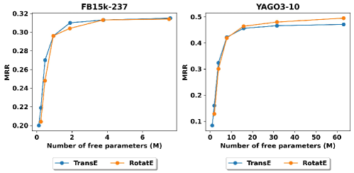
Figure 1: MRR versus the number of free parameters in KGE methods against FB15K-237 (left) and YAGO3-10 dataset (right). When a model has fewer parameters, its performance is poorer. Also, the larger dataset, YAGO3-10, demands more parameters than the smaller dataset, FB15k-237, to achieve satisfactory results.

Knowledge graph embedding (KGE) methods have been widely used to solve the incompleteness problem. Embeddings for entities and relations are stored as model parameters and updated by maximizing triple scores among observed triples while minimizing those among negative triples. The number of free parameters in a KGE model is linear to the embedding dimension and the number of entities and relations in KGs, i.e. $O((|E|+|R|)d)$, where $|E|$ is the number of entities, $|R|$ is the number of relations, and $d$ is the embedding dimension. Since KGE models usually require a higher-dimensional embedding space for a better reasoning capability, they require large model sizes (i.e. parameter numbers) to achieve satisfactory performance as demonstrated in Fig. 1. To this end, it is challenging for them to handle large-scale KGs with lots of entities and relations in resource-constrained platforms such as mobile/edge computing. A KGC method that has good reasoning capability in low dimensions is desired Kuo and Madni (2022).

The requirement of high-dimensional embeddings for popular KGE methods comes from the over-simplified scoring functions (Xiao et al., 2015). Thus, classification-based KGC methods, such as ConvE (Dettmers et al., 2018), aim to increase the reasoning capabilities in low dimensions by adopting neural networks (NNs) as powerful decoders. As a result, they are more efficient in parameter scaling than KGE models (Dettmers et al., 2018). However, NNs demand longer inference time and more computation power due to their deep architectures. The long inference time of the classification-based methods also limits their applicability to some tasks that require real-time inference. Recently, DualDE (Zhu et al., 2022) applied Knowledge Distillation (KD) (Hinton et al., 2015) to train powerful low-dimensional embeddings. Yet, it demands three stages of embedding training: 1) training high-dimensional KGE, 2) training low-dimensional KGE with the guidance of high-dimensional KGE, and 3) multiple rounds of student-teacher interactions. Its training process is time-consuming and may fail to converge when the embeddings are not well-initialized.

Here, we propose a new KGC method that works well under low dimensions and name it GreenKGC. GreenKGC consists of three modules: 1) representation learning, 2) feature pruning, and 3) decision learning. Each of them is trained independently. In Module 1, we leverage a KGE method, called the baseline method, to learn high-dimensional entity and relation representations. In Module 2, a feature pruning process is applied to the high-dimensional entity and relation representations to yield discriminant low-dimensional features for triples. In addition, we observe that some feature dimensions are more powerful than others in different relations. Thus, we group relations with similar discriminant feature dimensions for parameter savings and better performance. In Module 3, we train a binary classifier for each relation group so that it can predict triple’s score in inference. The score is a soft prediction between 0 and 1, which indicates the probability of whether a certain triple exists or not. Finally, we propose two novel negative sampling schemes, embedding-based and ontology-based, for classifier training in this work. They are used for hard negative mining, where these hard negatives cannot be correctly predicted by the baseline KGE methods.

We conduct extensive experiments and compare the performance and model sizes of GreenKGC with several representative KGC methods on link prediction datasets. Experimental results show that GreenKGC can achieve good performance in low dimensions, i.e. 8, 16, 32 dimensions, compared with SOTA low-dimensional methods. In addition, GreenKGC shows competitive or better performance compared to the high-dimensional KGE methods with a much smaller model size. We also conduct experiments on a large-scale link prediction datasets with over 2.5M entities and show that GreenKGC can perform well with much fewer model parameters. Ablation studies are also conducted to show the effectiveness of each module in GreenKGC.

2 Related Work

2.1 KGE Methods

Distance-based KGE methods model relations as affine transformations from head entities to tail entities. For example, TransE (Bordes et al., 2013) models relations as translations, while RotatE (Sun et al., 2019) models relations as rotations in the complex embedding space for better expressiveness on symmetric relations. Recent work has tried to model relations as scaling (Chao et al., 2021) and reflection (Zhang et al., 2022) operations in order to handle particular relation patterns. Semantic-matching KGE methods, such as RESCAL (Lin et al., 2015) and DistMult (Bordes et al., 2014), formulate the scoring functions as similarities among head, relation, and tail embeddings. ComplEx (Trouillon et al., 2016) extends such methods to a complex space for better expressiveness on asymmetric relations. Recently, TuckER (Balazevic et al., 2019) and AutoSF (Zhang et al., 2020) allow more flexibility in modeling similarities. Though KGE methods are simple, they often require a high-dimensional embedding space to be expressive.

2.2 Classification-based KGC Methods

NTN (Socher et al., 2013) adopts a neural tensor network combined with textual representations of entities. ConvKB (Nguyen et al., 2018) uses $1\times 3$ convolutional filters followed by several fully connected (FC) layers to predict triple scores. ConvE (Dettmers et al., 2018) reshapes entity and relation embeddings into 2D images and uses $3\times 3$ convolutional filters followed by several FC layers to predict the scores of triples. Though NN-based methods can achieve good performance in a lower dimension, they have several drawbacks, such as long inference time and large model. KGBoost (Wang et al., 2022) is a classification-based method that doesn’t use NNs. Yet, it assigns one classifier for each relation so it’s not scalable to large-scale datasets.

2.3 Low-dimensional KGE Methods

Recently, research on the design of low-dimensional KGE methods has received attention. MuRP (Balažević et al., 2019) embeds entities and relations in a hyperbolic space due to its effectiveness in modeling hierarchies in KGs. AttH (Chami et al., 2020) improves hyperbolic KGE by leveraging hyperbolic isometries to model logical patterns. MulDE (Wang et al., 2021) adopts Knowledge Distillation (Hinton et al., 2015) on a set of hyperbolic KGE as teachers to learn powerful embeddings in low dimensions. However, embeddings in hyperbolic space are hard to be used in other downstream tasks. In Euclidean space, DualDE (Zhu et al., 2022) adopts Knowledge Distillation to learn low-dimensional embeddings from high-dimensional ones for smaller model sizes and faster inference time. Yet, it requires a long training time to reduce feature dimension. GreenKGC has two clear advantages over existing low-dimensional methods. First, it fully operates in the Euclidean space. Second, it does not need to train new low-dimensional embeddings from scratch, thus requiring a shorter dimension reduction time.

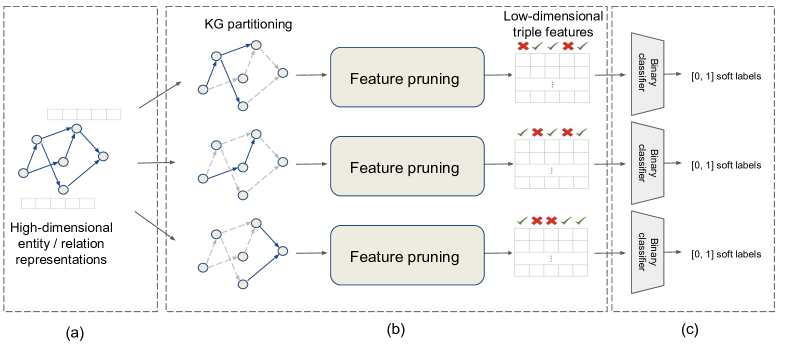
Figure 2: An overview of GreenKGC, which consists of three modules: (a) representation learning, (b) feature pruning, and (c) decision learning.

3 Methodology

GreenKGC is presented in this section. It consists of three modules: representation learning, feature pruning, and decision learning, to obtain discriminant low-dimensional triple features and predict triple scores accurately. An overview of GreenKGC is given in Fig. 2. Details of each module will be elaborated below.

3.1 Representation Learning

We leverage existing KGE models, such as TransE (Bordes et al., 2013) and RotatE (Sun et al., 2019), to obtain good initial embeddings for entities and relations, where their embedding dimensions can be high to be expressive. Yet, the initial embedding dimension will be largely reduced in the feature pruning module. In general, GreenKGC can build upon any existing KGE models. We refer to the KGE models used in GreenKGC as our baseline models. We include the training details for baseline models in Appendix 6.1 as they are not the main focus of this paper.

3.2 Feature Pruning

In this module, a small subset of feature dimensions in high-dimensional KG representations from Module 1 are preserved, while the others are pruned, to form low-dimensional discriminant KG features.

Discriminant Feature Test (DFT). DFT is a supervised feature selection method recently proposed in Yang et al. (2022). All training samples have a high-dimensional feature set as well as the corresponding labels. DFT scans through each dimension in the feature set and computes its discriminability based on sample labels. DFT can be used to reduce the dimensions of entity and relation embeddings while preserving their power in downstream tasks such as KGC.

Here, we extend DFT to the multivariate setting since there are multiple variables in each triple. For example, TransE (Bordes et al., 2013) has 3 variables (i.e. $\bm{h}$, $\bm{r}$, and $\bm{t}$) in each feature dimension. First, for each dimension $i$, we learn a linear transformation $\bm{w}_{i}$ to map multiple variables $[h_{i},r_{i},t_{i}]$ to a single variable $x_{i}$ in each triple, where $h_{i},r_{i},t_{i}$ represents the $i$-th dimension in the head, relation, and tail representations, respectively. Such a linear transformation can be learned through principal component analysis (PCA) using singular value decomposition (SVD). As a result, $\bm{w}_{i}$ is the first principal component in PCA. However, linear transformations learned from PCA are unsupervised and cannot separate observed triples from negatives well. Alternatively, we learn the linear transformation through logistic regression by minimizing the binary cross-entropy loss

$$\begin{split}\mathcal{L}={}&-y\log(\sigma(\bm{w}_{i}[h_{i},r_{i},t_{i}]^{T}))\\ &-(1-y)\log(1-\sigma(\bm{w}_{i}[h_{i},r_{i},t_{i}]^{T})),\end{split}$$ (1)

where $y=1$ for observed triples $(h,r,t)$ and $y=0$ for corrupted triples $(h^{\prime},r,t^{\prime})$. Afterward, we can apply the standard DFT to each dimension.

DFT adopts cross-entropy (CE) to evaluate the discriminant power of each dimension as CE is a typical loss for binary classification. Dimensions with lower CE imply higher discriminant power. We preserve the feature dimensions with the lowest CE and prune the remaining to obtain low-dimensional features. Details for training DFT are given in Appendix 6.2.

KG partitioning. Given that relations in KGs could be different (e.g. symmetric v.s. asymmetric and films v.s. sports), a small subset of feature dimensions might not be discriminant for all relations. Thus, we first partition them into disjoint relations groups, where relations in each group have similar properties. Then, we perform feature pruning within each relation group and select the powerful feature dimensions correspondingly.

Cluster #	Relations
0	_derivationally_related_form
	_also_see
	_member_meronym
	_has_part
	_verb_group
	_similar_to
1	_hypernym
	_instance_hypernym
	_synset_domain_topic_of
2	_member_of_domain_usage
	_member_of_domain_region

Table 1: Relation grouping results on WN18RR when applying $k$-Means on relation embeddings when $k$ = 3.

We hypothesize that relations that have similar properties are close in the embedding space. Therefore, we use $k$-Means to cluster relation embeddings into relation groups. To verify our hypothesize, we show the grouping results on WN18RR in Table 1. Without categorizing relations into different logical patterns explicitly, relations of similar patterns can be clustered together in the embedding space. For example, most relations in cluster #0 are symmetric ones. All relations in the cluster #1 are N-to-1. The remaining two relations in cluster #2 are 1-to-N with the highest tail-per-head ratio. While we observe cardinality-based grouping for relations in WN18RR, which mostly contains abstract concepts, for FB15k-237 and YAGO3-10, relations with similar semantic meanings are often grouped after KG partitioning.

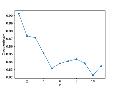
Figure 3: Average cross-entropy for different numbers of KG partitions in FB15k-237.

Furthermore, we evaluate how different numbers of relation groups, $k$, can affect the feature pruning process. In Fig. 3, as the lower CE reflects more discriminant features, we can obtain more powerful features when $k$ becomes larger, i.e. partitioning KG into more relation groups. Thus, for each dataset, we select the optimal $k$ when the average CE starts to converge. We elaborate on the high-level intuition on why combining feature pruning and KG partitioning works with KGE models. First, KGE models are isotropic, meaning each dimension can be handled by DFT independently. Second, some feature dimensions are more powerful than others in different relations. Thus, we group relations that with the same discriminant feature dimensions for parameter savings.

3.3 Decision Learning

We formulate KGC as a binary classification problem in each relation group. We adopt binary classifiers as decoders since they are more powerful than simple scoring functions. The binary classifiers take pruned triple features as inputs and predict soft probabilities (between 0 and 1) of triples as outputs. We also conduct classifier training with hard negative mining so as to train a powerful classifier.

Binary classification. The binary classifiers, $g(*)$, take a low-dimensional triple feature $\bm{x}$ and predict a soft label $\hat{y}=g(\bm{x})\in[0,1]$. The label $y=1$ for the observed triples and $y=0$ for the sampled negatives. We train a binary classifier by minimizing the following negative log-likelihood loss:

$$\begin{split}l(y,\hat{y})={}&-y\log(\hat{y})\\ &-(1-y)\log(1-\hat{y}),\end{split}$$ (2)

In general, we select a nonlinear classifier to accommodate nonlinearity in sample distributions.

Negative sampling. Combining KGE with classifiers is non-trivial because it’s challenging to obtain high-quality negative samples for classifier training, given that negative samples are not explicitly labeled in the KGs. Therefore, it is desired to mine hard negative cases for baseline KGE models so as to train a powerful classifier. We propose two negative sampling schemes for classifier training. First, most KGE models can only capture the coarse entity type information. For example, they may predict a location given the query (Mary, born_in, ?) yet without an exact answer. Thus, we draw negative samples within the entity types constrained by relations (Krompaß et al., 2015) to enhance the capability to predict the exact answer. Such a negative sampling scheme is called ontology-based negative sampling. We also investigate the sampling of hard negatives that cannot be trivially obtained from original KGE methods. Negatives with higher embedding scores $f_{r}(\bm{h_{i}},\bm{t_{i}})$ tend to be predicted wrongly in the baseline methods. To handle it, we rank all randomly sampled negative triples and select the ones with higher embedding scores as hard negatives for classifier training. Such a negative sampling strategy is called embedding-based negative sampling.

4 Experiments

Dataset	# ent.	# rel.	# triples (train / valid / test)
WN18RR	40,943	11	86,835 / 3,034 / 3,134
FB15k-237	14,541	237	272,115 / 17,535 / 20,466
YAGO3-10	123,143	37	1,079,040 / 4,978 / 4,982
ogbl-wikikg2	2,500,604	535	16,109,182 / 429,456 / 598,543

Table 2: Dataset statistics.

	FB15k-237				WN18RR				YAGO3-10
Model	MRR	H@1	H@3	H@10	MRR	H@1	H@3	H@10	MRR	H@1	H@3	H@10
KGE Methods
TransE (Bordes et al., 2013)	0.270	0.177	0.303	0.457	0.150	0.009	0.251	0.387	0.324	0.221	0.374	0.524
RotatE (Sun et al., 2019)	0.290	0.208	0.316	0.458	0.387	0.330	0.417	0.491	0.419	0.321	0.475	0.607
Classification-based Methods
ConvKB (Nguyen et al., 2018)	0.232	0.157	0.255	0.377	0.346	0.300	0.374	0.422	0.311	0.194	0.368	0.526
ConvE (Dettmers et al., 2018)	0.282	0.201	0.309	0.440	0.405	0.377	0.412	0.453	0.361	0.260	0.396	0.559
Low-dimensional Methods
MuRP (Balažević et al., 2019)	0.323	0.235	0.353	0.501	0.465	0.420	0.484	0.544	0.230	0.150	0.247	0.392
AttH (Chami et al., 2020)	0.324	0.236	0.354	0.501	0.466	0.419	0.484	0.551	0.397	0.310	0.437	0.566
DualDE (Zhu et al., 2022)	0.306	0.216	0.338	0.489	0.468	0.419	0.486	0.560	-	-	-	-
TransE + GreenKGC (Ours)	0.331	0.251	0.356	0.493	0.342	0.300	0.365	0.413	0.362	0.265	0.408	0.537
RotatE + GreenKGC (Ours)	0.345	0.265	0.369	0.507	0.411	0.367	0.430	0.491	0.453	0.361	0.509	0.629

Table 3: Results of link prediction in low dimensions ($d=32$), where the best and the second best numbers are in bold and with an underbar, respectively.

4.1 Experimental Setup

Datasets. We consider four link prediction datasets for performance benchmarking: FB15k-237 (Bordes et al., 2013; Toutanova and Chen, 2015), WN18RR (Bordes et al., 2013; Dettmers et al., 2018), YAGO3-10 (Dettmers et al., 2018), and ogbl-wikikg2 (Hu et al., 2020). Their statistics are summarized in Table 2. FB15k-237 is a subset of Freebase (Bollacker et al., 2008) that contains real-world relationships. WN18RR is a subset of WordNet (Miller, 1995) containing lexical relationships between word senses. YAGO3-10 is a subset of YAGO3 (Mahdisoltani et al., 2014) that describes the attributes of persons. ogbl-wikikg2 is extracted from wikidata (Vrandečić and Krötzsch, 2014) capturing the different types of relations between entities in the world. Among the four, ogbl-wikikg2 is a large-scale dataset with more than 2.5M entities.

Implementation details. We adopt TransE (Bordes et al., 2013) and RotatE (Sun et al., 2019) as the baseline models and learn 500 dimensions initial representations for entities and relations. The feature dimensions are then reduced in the feature pruning process. We compare among GreenKGC using RotatE as the baseline in all ablation studies. To partition the KG, we determine the number of groups $k$ for each dataset when the average cross-entropy of all feature dimensions converges. As a result, $k=3$ for WN18RR, $k=5$ for FB15k-237 and YAGO3-10, and $k=20$ for ogbl-wikikg2.

For decision learning, we consider several tree-based binary classifiers, including Decision Trees (Breiman et al., 2017), Random Forest (Breiman, 2001), and Gradient Boosting Machines (Chen and Guestrin, 2016), as they match the intuition of the feature pruning process and can accommodate non-linearity in the sample distribution. The hyperparameters are searched among: tree depth $l\in$ {3, 5, 7}, number of estimators $n\in$ {400, 800, 1,200, 1,600, 2,000}, and learning rate $lr\in$ {0.05, 0.1, 0.2}. The best settings are chosen based on MRR in the validation set. As a result, we adopt Gradient Boosting Machine for all datasets. $l=5$, $n=1200$, $lr=0.2$ for FB15k-237 and YAGO3-10, $l=3$, $n=1600$, $lr=0.1$ for WN18RR, and $l=7$, $n=2000$, $lr=0.05$ for ogbl-wikikg2. We adopt ontology-based negative sampling to train classifiers for FB15k-237, YAGO3-10, and ogbl-wikikg2, and embedding-based negative sampling for WN18RR. Baseline KGEs are trained on NVIDIA Tesla P100 GPUs and binary classifiers are trained on AMD EPYC 7542 CPUs.

Evaluation metrics. For the link prediction task, the goal is to predict the missing entity given a query triple, i.e. $(h,r,?)$ or $(?,r,t)$. The correct entity should be ranked higher than other candidates. Here, several common ranking metrics are used, such as MRR (Mean Reciprocal Rank) and Hits@k (k=1, 3, 10). Following the convention in Bordes et al. (2013), we adopt the filtered setting, where all entities serve as candidates except for the ones that have been seen in training, validation, or testing sets.

		FB15k-237			WN18RR			YAGO3-10
Baseline	Dim.	MRR	H@1	#P (M)	MRR	H@1	#P (M)	MRR	H@1	#P (M)
TransE	500	0.325	0.228	7.40	0.223	0.013	20.50	0.416	0.319	61.60
	100	0.274	0.186	1.48	0.200	0.009	4.10	0.377	0.269	12.32
		$\downarrow$ 15.7%	$\downarrow$ 18.5%	(0.20x)	$\downarrow$ 10.3%	$\downarrow$ 30.8%	(0.20x)	$\downarrow$ 9.4%	$\downarrow$ 16.7%	(0.20x)
	100	0.338	0.253	1.76	0.407	0.361	4.38	0.455	0.358	12.60
	(Ours)	$\uparrow$ 4.0%	$\uparrow$ 9.6%	(0.24x)	$\uparrow$ 82.5%	$\uparrow$ 176.9%	(0.21x)	$\uparrow$ 9.4%	$\uparrow$ 12.2%	(0.20x)
RotatE	500	0.333	0.237	14.66	0.475	0.427	40.95	0.478	0.388	123.20
	100	0.296	0.207	2.93	0.437	0.385	8.19	0.432	0.340	24.64
		$\downarrow$ 11.1%	$\downarrow$ 12.7%	(0.20x)	$\downarrow$ 8%	$\downarrow$ 9.8%	(0.20x)	$\downarrow$ 9.6%	$\downarrow$ 12.4%	(0.20x)
	100	0.348	0.266	3.21	0.458	0.424	8.47	0.467	0.378	24.92
	(Ours)	$\uparrow$ 4.5%	$\uparrow$ 12.2%	(0.22x)	$\downarrow$ 3.6%	$\downarrow$ 0.7%	(0.21x)	$\downarrow$ 2.3%	$\downarrow$ 3.6%	(0.20x)

Table 4: Results on the link prediction task, where we show the performance gain (or loss) in terms of percentages with an up (or down) arrow and the ratio of the model size within the parentheses against those of respective 500-dimensional models.

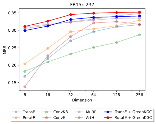
Figure 4: Embedding dimension $d$ to MRR curves in log-scale for various methods on FB15k-237. $d$ = 8, 16, 32, 64, 128, 256.

4.2 Main Results

Results in low dimensions. In Table 3, we compare GreenKGC with KGE, classification-based, and low-dimensional KGE methods in low dimensions, i.e. $d$ = 32. Results for other methods in Table 3 are either directly taken from (Chami et al., 2020; Zhu et al., 2022) or, if not presented, trained by ourselves using publicly available implementations with hyperparameters suggested by the original papers. KGE methods cannot achieve good performance in low dimensions due to over-simplified scoring functions. Classification-based methods achieve performance better than KGE methods as they adopt NNs as complex decoders. Low-dimensional KGE methods provide state-of-the-art KGC solutions in low dimensions. Yet, GreenKGC outperforms them in FB15k-237 and YAGO3-10 in all metrics. For WN18RR, the baseline KGE methods perform poorly in low dimensions. GreenKGC is built upon KGEs, so this affects the performance of GreenKGC in WN18RR. Thus, GreenKGC is more suitable for instance-based KGs, such as Freebase and YAGO, while hyperbolic KGEs, such as MuRP and AttH model the concept-based KGs, such as WordNet, well.

We show the performance curves of various methods as a function of embedding dimensions in Fig. 4. We see that the performance of KGE methods (i.e. TransE and RotatE) drops significantly as the embedding dimension is lower. For ConvKB, although its performance is less influenced by dimensions due to a complex decoder, it performs poorly compared to other methods in general. For ConvE, although it claims it’s more efficient in parameter scaling (Dettmers et al., 2018), its performance actually degrades significantly in dimensions lower than 64. In addition, it also doesn’t perform well when the dimension is larger. Thus, the performance of ConvE is sensitive to the embedding dimension. MuRP, AttH, and GreenKGC are the only methods that can offer reasonable performance as the dimension goes to as low as 8 dimensions.

Method	#P (M)	Val. MRR	Test MRR
TransE (d = 500)	1,250 (5$\times$)	0.427	0.426
RotatE (d = 250)	1,250 (5$\times$)	0.435	0.433
TransE (d = 100)	250 (1$\times$)	0.247	0.262
TransE + GreenKGC (d = 100)	250 (1$\times$)	0.339	0.331
RotatE (d = 50)	250 (1$\times$)	0.225	0.253
RotatE + GreenKGC (d = 50)	250 (1$\times$)	0.341	0.336

Table 5: Link prediction performance on obgl-wikikg2 dataset.

Comparison with baseline KGE. One unique characteristic of GreenKGC is to prune a high-dimensional KGE into low-dimensional triple features and make predictions with a binary classifier as a powerful decoder. We evaluate the capability of GreenKGC in saving the number of parameters and maintaining the performance by pruning original 500-dimensional KGE to 100-dimensional triple features in Table 4. As shown in the table, GreenKGC can achieve competitive or even better performance with around 5 times smaller model size. Especially, Hits@1 is retained the most and even improved compared to the high-dimensional baselines. In addition, GreenKGC using TransE as the baseline can outperform high-dimensional TransE in all datasets. Since the TransE scoring function is simple and fails to model some relation patterns, such as symmetric relations, incorporating TransE with a powerful decoder, i.e. a binary classifier, in GreenKGC successfully overcomes deficiencies of adopting an over-simplified scoring function. For all datasets, 100-dimensional GreenKGC could generate better results than 100-dimensional baseline models.

We further compare GreenKGC and its baseline KGEs on a large-scale dataset, ogbl-wikikg2. Table 5 shows the results. We reduce the feature dimensions from 500 to 100 for RotatE and 250 to 50 for TransE and achieve a 5x smaller model size while retaining around 80% of the performance. Compared with the baseline KGEs in the same feature dimension, GreenKGC can improve 51.6% in MRR for RotatE and 37.2% in MRR for TransE. Therefore, the results demonstrate the advantages in performance to apply GreenKGC to large-scale KGs in a constrained resource.

4.3 Ablation Study

	FB15k-237			WN18RR
	MRR	H@1	H@10	MRR	H@1	H@10
w/o pruning	0.318	0.243	0.462	0.379	0.346	0.448
random	0.313	0.239	0.460	0.375	0.346	0.420
variance	0.315	0.239	0.465	0.381	0.348	0.455
feature importance	0.323	0.241	0.478	0.385	0.355	0.464
prune low CE	0.312	0.236	0.460	0.373	0.343	0.419
prune high CE (Ours)	0.345	0.265	0.507	0.411	0.367	0.491

Table 6: Performance for RotatE + GreenKGC in 32 dimensions with different feature pruning scheme.

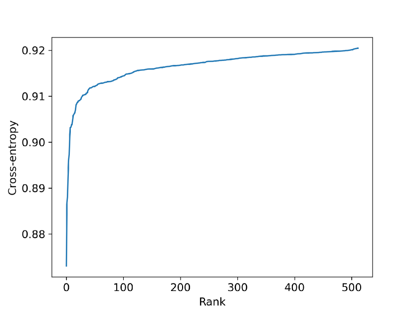
(a) Cross-entropy in DFT

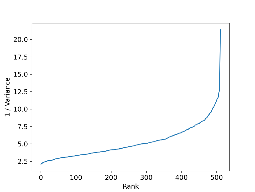
(b) 1 / Variance

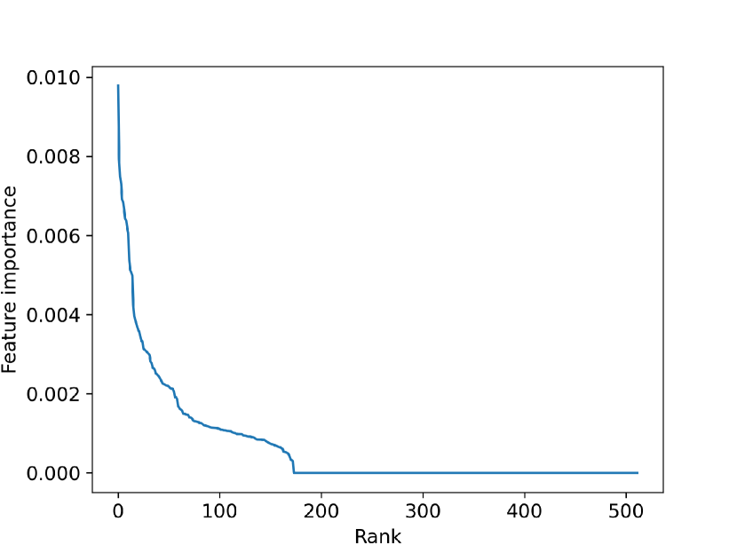
(c) Feature importance

Figure 5: Sorted discriminability for each feature dimension in different feature pruning schemes. For cross-entropy and 1/variance, a lower value indicates a more discriminant feature. For feature importance, a higher value indicates a more discriminant feature.

Feature pruning. We evaluate the effectiveness of the feature pruning scheme in GreenKGC in Table 6. We use “w/o pruning" to denote the baseline 32 dimensions KGE directly followed by the decision learning module. Also, we compare the following feature pruning schemes: 1) random pruning, 2) pruning based on variance, 3) pruning based on feature importance from a Random Forest classifier, 4) pruning dimensions with low CE (i.e. the most discriminant ones), in DFT, and 5) pruning dimensions with high CE (i.e. the least discriminant ones) in DFT. As shown in the table, our method to prune the least discriminant features in DFT achieves the best performance on both datasets. In contrast, pruning the most discriminant features in DFT performs the worst. Thus, DFT module can effectively differentiate the discriminability among different features. Using variance to prune achieves similar results as “w/o pruning" and random pruning. Pruning based on feature importance shows better results than “w/o pruning", random and pruning, and pruning based on variance, but performs worse than DFT. In addition, feature importance needs to consider all feature dimensions at once, while in DFT, each feature dimension is processed individually. Thus, DFT is also more memory efficient than calculating feature importance.

Fig. 5 plots the sorted discriminability of features in different pruning schemes. From the figure, the high variance region is flat, so it’s difficult to identify the most discriminant features using their variances. For feature importance, some of the feature dimensions have zero scores. Therefore, pruning based on feature importance might ignore some discriminant features. In the DFT curve, there is a “shoulder point" indicating only around 100 feature dimensions are more discriminant than the others. In general, we can get good performance in low dimensions as long as we preserve dimensions lower than the shoulder point and prune all other dimensions.

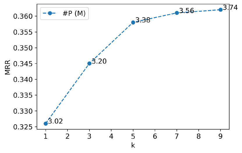
(a) FB15k-237

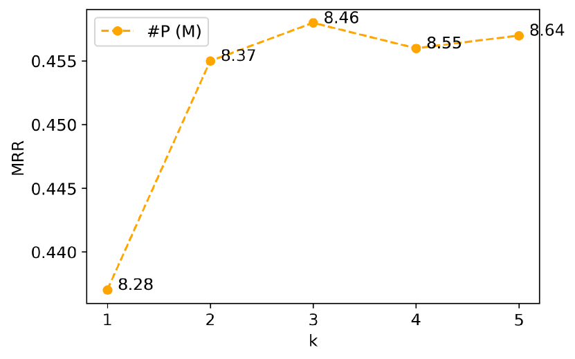
(b) WN18RR

Figure 6: Ablation study on number of relation groups $k$ to MRR.

KG partitioning. Figure 6 shows GreenKGC performance with different numbers of relation groups $k$, where $k=1$ means no KG partitioning. A larger $k$ will give a better performance on both FB15k-237 and WN18RR. Without using KG partitioning performs much worse than using KG partitioning. Note that with a larger $k$, GreenKGC has more model parameters since we need more classifiers. The model complexity is $O(|E|d+k\Theta)$, where $\Theta$ is the model complexity for the classifier. Thus, we can adjust $k$ based on the tradeoff of performance convergence and memory efficiency.

5 Conclusion and Future Work

A lightweight KGC method, called GreenKGC, was proposed in this work to make accurate link predictions in low dimensions. It consists of three modules that can be trained individually: 1) representation learning, 2) feature pruning, and 3) decision learning. Experimental results in low dimensions demonstrate GreenKGC can achieve satisfactory performance in as low as 8 dimensions. In addition, experiments on ogbl-wikikg2 show GreenKGC can get competitive results with much fewer model parameters. Furthermore, the ablation study shows the effectiveness of KG partitioning and feature pruning.

Modularized GreenKGC allows several future extensions. First, GreenKGC can be combined with new embedding models as initial features. In general, using a more expressive KGE model can lead to better final performance. Second, individual modules can be fine-tuned for different applications. For example, since the feature pruning module and the decision-learning module are supervised, they can be applied to various applications. Finally, different negative sampling strategies can be investigated in different applications.

6 Appendix

6.1 Training Procedure for Baseline KGE Models

Model	$n_{e}$	$n_{r}$	$n_{v}$	$f_{r}(h,t)$
TransE	1	1	3	$-\|\bm{h}+\bm{r}-\bm{t}\|$
DistMult	1	1	3	$\langle\bm{h},\bm{r},\bm{t}\rangle$
ComplEx	2	2	6	$Re(\langle\bm{h},\bm{r},\overline{\bm{t}}\rangle)$
RotatE	2	1	5	$-\|\bm{h}\circ\bm{r}-\bm{t}\|^{2}$

Table 7: Popular KGE methods and their scoring functions, where $\bm{h}$, $\bm{r}$, and $\bm{t}$ denote embeddings for a given triple $(h,r,t)$, $d$ is the embedding dimension. $\circ$ denotes the Hadamard product, and $\langle\cdot,\cdot,\cdot\rangle$ is the generalized dot product. $n_{e}$ is the number of entity variables in one dimension, $n_{r}$ is the number of relation variables in one dimension, and $n_{v}$ is the number of triple variables in one dimension. $n_{v}=2n_{e}+n_{r}$.

To train the baseline KGE model as the initial entity and relation representations, we adopt the self-adversarial learning process in Sun et al. [2019] and use this codebase. That is, given an observed triple $(h,r,t)$ and the KGE model $f_{r}(\bm{h},\bm{t})$, we minimize the following loss function

$$\begin{split}\mathcal{L}={}&-\log(\sigma(f_{r}(\bm{h},\bm{t})))\\ &-\sum_{i=1}^{n}p(h^{\prime}_{i},r,t^{\prime}_{i})\log(\sigma(-f_{r}(\bm{h}^{\prime}_{i},\bm{t}^{\prime}_{i}))),\end{split}$$ (3)

where $(h^{\prime}_{i},r,t^{\prime}_{i})$ is a negative sample and

$$p(h^{\prime}_{j},r,t^{\prime}_{j})=\frac{\exp(\alpha f_{r}(\bm{h}^{\prime}_{j},\bm{t}^{\prime}_{j}))}{\sum_{i=1}^{n}\exp(\alpha f_{r}(\bm{h}^{\prime}_{i},\bm{t}^{\prime}_{i}))},$$ (4)

where $\alpha$ is the temperature to control the self-adversarial negative sampling. We summarize the scoring functions for some common KGE models and their corresponding number of variables per dimension in Table 7. In general, GreenKGC can build upon any existing KGE models.

6.2 DFT Implementation Details

To calculate the discriminant power of each dimension, we iterate through each dimension in the high-dimension feature set and calculate the discriminant power based on sample labels. More specifically, we model KGC as a binary classification task. We assign label $y_{i}=1$ to the $i$th sample if it is an observed triple and $y_{i}=0$ if it is a negative sample. For the $d$th dimension, we split the 1D feature space into left and right subspaces and calculate the cross-entropy in the form of

$$H^{(d)}=\frac{N_{L}H_{L}^{(d)}+N_{R}H_{R}^{(d)}}{N_{L}+N_{R}},$$ (5)

where $N_{L}$ and $N_{R}$ are the numbers of samples in the left and right intervals, respectively,

$$H_{L}^{(d)}=-P_{L,1}\log(P_{L,1})-P_{L,0}\log(P_{L,0}),$$ (6)

$$H_{R}^{(d)}=-P_{R,1}\log(P_{R,1})-P_{R,0}\log(P_{R,0}),$$ (7)

and where $P_{L,1}=\frac{1}{N_{L}}\sum_{i=1}^{N_{L}}y_{i}$, and $P_{L,0}=1-P_{L,1}$ and similarly for $P_{R,1}$ and $P_{R,0}$. A lower cross-entropy value implies higher discriminant power.

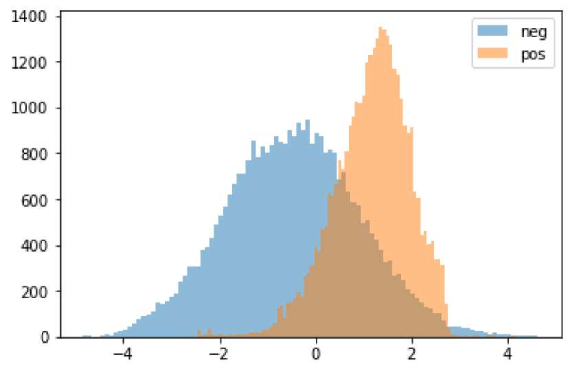
(a) Cross-entropy $=0.7348$

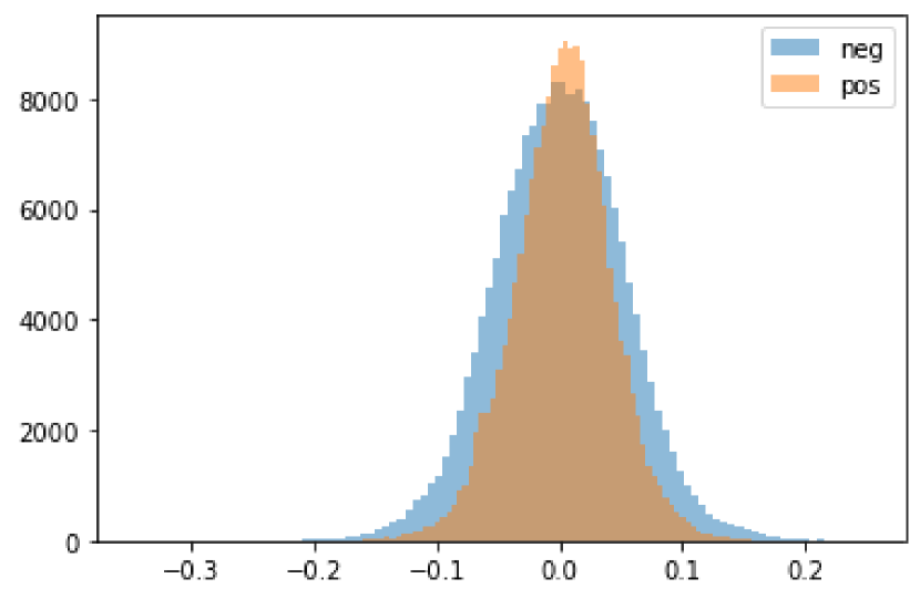
(b) Cross-entropy $=0.9910$

Figure 7: Histograms of PCA-transformed 1D triple variables in two feature dimensions with (a) low and (b) high cross-entropy.

Fig. 7 shows histograms of linearly transformed 1D triple variables in two different feature dimensions. As seen in the figure, samples in Fig. 7 (a), i.e. the feature dimension with the lower cross-entropy, are more separable than that in Fig. 7 (b), i.e. the feature dimension with the higher cross-entropy. Therefore, a lower cross-entropy implies a more discriminant feature dimension.

	Predicting Heads				Predicting Tails
Model	1-to-1	1-to-N	N-to-1	N-to-N	1-to-1	1-to-N	N-to-1	N-to-N
TransE Bordes et al. [2013]	0.374	0.417	0.037	0.217	0.372	0.023	0.680	0.322
RotatE Sun et al. [2019]	0.468	0.431	0.066	0.229	0.463	0.057	0.725	0.336
AttH Chami et al. [2020]	0.473	0.432	0.071	0.236	0.472	0.057	0.728	0.343
TransE + GreenKGC (Ours)	0.478	0.442	0.088	0.243	0.477	0.096	0.754	0.351
RotatE + GreenKGC (Ours)	0.483	0.455	0.134	0.245	0.486	0.112	0.765	0.353

Table 8: Performance on different relation categories in FB15k-237 under 32 dimensions.

6.3 Relation Categories

We further evaluate GreenKGC in different relation categories. Following the convention in Wang et al. [2014], we divide the relations into four categories: 1-to-1, 1-to-N, N-to-1, and N-to-N. They are characterized by two statistical numbers, head-per-tail (hpt), and tail-per-head (tph), of the datasets. If $tph<1.5$ and $hpt<1.5$, the relation is treated as 1-to-1; if $tph<1.5$ and $hpt\geq 1.5$, the relation is treated as 1-to-N; if $tph\geq 1.5$ and $hpt<1.5$, the relation is treated as N-to-1; if $tph\geq 1.5$ and $hpt\geq 1.5$, the relation is treated as N-to-N.

Table 8 summarizes the results for different relation categories in FB15k-237 under 32 dimensions. In the low-dimensional setting, GreenKGC is able to outperform other methods in all relation categories. Specifically, GreenKGC performs especially well for many-to-1 predictions (i.e. predicting heads for 1-to-N relations, and predicting tails for N-to-1 relations). Such results demonstrate the advantage of using classifiers to make accurate predictions when there is only one valid target.

	FB15k-237	WN18RR	YAGO3-10
DualDE	03:30:50	01:50:00	09:28:20
GreenKGC (Ours)	00:10:50	00:06:02	00:23:35

Table 9: Comparison of required training time (Hour : Minute : Second) to reduce the feature dimensions from 512 to 100 for TransE between DualDE, a knowledge-distillation method, and GreenKGC.

	FB15k-237						WN18RR
Model	MRR	H@1	H@3	H@10	#P (M)	T (s)	MRR	H@1	H@3	H@10	#P (M)	T (s)
ConvKB [Nguyen et al., 2018]	0.258	0.179	0.283	0.416	1.91	548.67	0.369	0.317	0.399	0.468	5.26	225.12
ConvE [Dettmers et al., 2018]	0.317	0.230	0.347	0.493	2.74	235.73	0.427	0.394	0.437	0.495	6.09	46.08
TransE + GreenKGC (Ours)	0.339	0.253	0.364	0.503	2.42	205.12	0.435	0.391	0.461	0.510	5.84	40.01

Table 10: Comparison on performance, number of model parameters, and total inference time (batch size = 8) with other classification-based methods in 128 dimensions. We adopt TransE as the baseline for fair comparison in the number of model parameters. The best numbers are in bold.

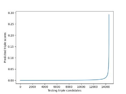
Figure 8: Prediction distribution of a query (38th Grammy Awards, award_winner, ?) in FB15k-237. A higher predicted score implies a higher chance of being a valid triple.

	FB15k-237			WN18RR
Neg. sampling	MRR	H@1	H@10	MRR	H@1	H@10
Random	0.283	0.197	0.452	0.407	0.361	0.481
Ontology	0.345	0.265	0.507	0.403	0.350	0.487
Embedding	0.316	0.232	0.471	0.411	0.367	0.491

Table 11: Ablation study on different negative sampling methods for classifier training in 32 dimensions.

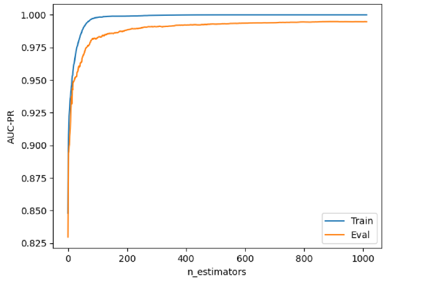
(a) Training/evaluation AUC-PR.

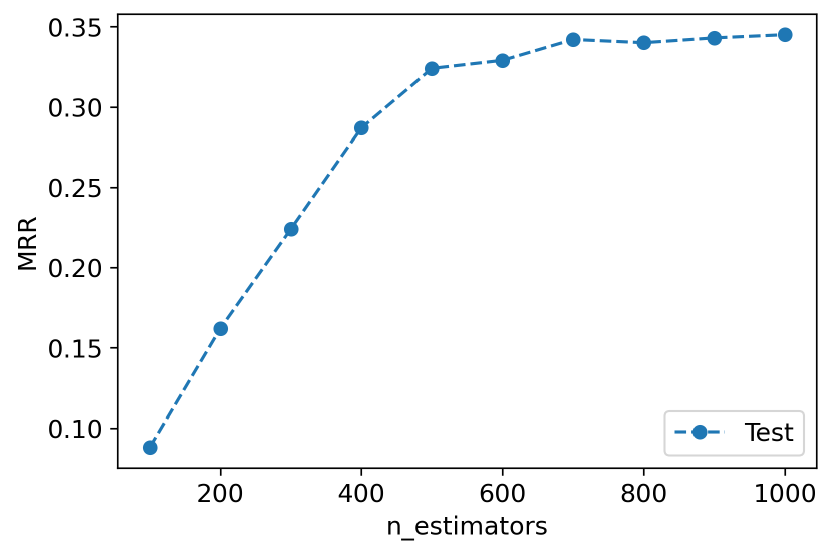
(b) Testing MRR.

Figure 9: Training/evaluation AUC-PR and testing MRR to the number of training iterations.

6.4 Time Analysis on Feature Pruning

Table 9 shows the required training time for DualDE [Zhu et al., 2022], a knowledge distillation method, and GreenKGC, to reduce 512 dimensions TransE embeddings to 100 dimensions. As shown in the table, GreenKGC achieves around 20x faster training time compared to DualDE, especially in YAGO3-10, which is a larger-scale dataset. Besides, in knowledge distillation methods, low-dimensional embeddings are randomly initialized and trained with the guidance of high-dimensional embeddings. Thus, the quality of the low-dimensional embeddings highly depends on good initialization. On the contrary, the feature pruning process in GreenKGC selects a subset of powerful feature dimensions without learning new features from scratch. In addition, it is also memory-efficient since it only processes one feature dimension at once.

6.5 Comparison with NN-based Methods

Inference time analysis. We compare GreenKGC with two other NN-based methods in Table 10 in terms of performance, number of free parameters, and inference time. They are ConvKB [Nguyen et al., 2018] and ConvE [Dettmers et al., 2018]. We adopt TransE as the baseline in GreenKGC to match the number of parameters in the embedding layer for a fair comparison. As compared with ConvKB, GreenKGC achieves significantly better performance with slightly more parameters. As compared with ConvE, GreenKGC uses fewer parameters and demands a shorter inference time since ConvE adopts a multi-layer architecture. GreenKGC also offers better performance compared to ConvE.

Prediction distribution. It was reported in Sun et al. [2020] that the predicted scores for all candidates on FB15k-237 are converged to 1 with ConvKB [Nguyen et al., 2018]. This is unlikely to be true, given the fact that KGs are often highly sparse. The issue is resolved after ConvKB is implemented with PyTorch, but the performance on FB15k-237 is still not as good as ConvKB originally reported in the paper. The issue shows the problem of end-to-end optimization. That is, it is difficult to control and monitor every component in the model. This urges us to examine whether GreenKGC has the same issue. Fig. 8 shows the sorted predicted scores of a query (38th Grammy Awards, award_winner, ?) in FB15k-237. We see from the figure that only very few candidates have positive scores close to $1$, while other candidates receive negative scores of 0. The formers are valid triples. The score distribution is consistent with the sparse nature of KGs.

6.6 Ablation on Negative Sampling

We evaluate the effectiveness of the two proposed negative sampling (i.e., ontology- and embedding-based) methods in Table 11. In FB15k-237, both are more effective than randomly drawn negative samples. The ontology-based one gives better results than the embedding-based one. In WN18RR, the embedding-based one achieves the best results. Since there is no clear entity typing in WordNet, the ontology-based one performs worse than the randomly drawn one. We can conclude that to correct failure cases in the baseline KGE, ontology-based negative sampling is effective for KGs consisting of real-world instances, such as FB15k-237, while embedding-based negative sampling is powerful for concept KGs such as WN18RR.

6.7 Performance as Training Progresses

We plot the AUC-PR and MRR curve for training/validation, and testing in Fig. 9(a) and Fig. 9(b), respectively. We use AUC-PR to monitor the training of the classifiers. AUC-PR starts to converge for both training and validation sets after 200 iterations. We record the link prediction results on the testing set every 100 iterations. Though the AUC-PR improves slightly after 200 iterations, the MRR starts to converge after 600 iterations.