Averaged Recurrence Quantification Analysis

Abstract

Recurrence quantification analysis (RQA) is a well established method of nonlinear data analysis. In this work we present a new strategy for an almost parameter-free RQA. The approach finally omits the choice of the threshold parameter by calculating the RQA measures for a range of thresholds (in fact recurrence rates). Specifically, we test the ability of the RQA measure determinism, to sort data with respect to their signal to noise ratios. We consider a periodic signal, simple chaotic logistic equation, and Lorenz system in the tested data set with different and even very small signal to noise ratios of lengths $10^{2},10^{3},10^{4},$ and $10^{5}$. To make the calculations possible a new effective algorithm was developed for streamlining of the numerical operations on Graphics Processing Unit (GPU).

1 Introduction

The authors in Bradley and Kantz (2015) wrote in the very end: “Will it be possible to design algorithms whose free parameters can be chosen systematically, via intuition, or perhaps even automatically? Such developments would streamline nonlinear time-series analysis, making it an indispensible tool to make sense out of the real world.” In this article we present a way of reducing the effect of a specific choice of the important threshold parameter in the well established nonlinear method of recurrence quantification analysis (RQA).

The popularity of RQA is continuously increasing in many fields across the science spectra – physical, biological, economical, simply everywhere where data can be obtainedWebber and Marwan (2015).

There is yet an open question on the selection of the basic parameter needed for the calculation of the recurrence plot (RP), the base of the RQA. The RP needs for its calculations a threshold parameter, $\varepsilon$, those selection can influence the results but depends on the specific research questionMarwan (2011). The choice of $\varepsilon$ was already discussed in previous studies Thiel et al. (2002); Medrano et al. (2021); Andreadis et al. (2020); Schinkel et al. (2008).

In this work we propose and study the possibility of providing RQA in a different way by omitting the choice of single $\varepsilon$ and, thus, making RQA more stable and objective. Here we use RQA for comparing data with different amounts of noise, where the deterministic behaviour in time series can be reflected at more scales Cencini et al. (2000), corresponding, e.g., to different thresholds $\varepsilon$. Therefore, we use a set of $\varepsilon$ values corresponding to a given set of recurrence rates (RRs) while we test the assumption that averaging the RQA resulting by the selected RRs improves the analysis. We provide the testing for various types of data of different lengths to study also the relation with the amount of data points needed in order to sort them according to its deterministic content. The data have different signal-to-noise ratios while we focus on the RQA measure determinism (DET) in order to explore the ability to recognize deterministic structures and evaluate quantitatively the amount of contaminating noise.

In order for the numerical tests to be carried out in an acceptable amount of time, we perform the RQA calculation on a Graphics Processing Unit (GPU) which also significantly enlarges the possible dimensions of the input time series for RQA due to the effective memory handling. This new computation method opens the door for desktop computers to perform RQA for large data alongside with the proposed novel approach to deliver more robust results.

When analysing time series from experiments or real world applications, it is difficult to distinguish between deterministic chaos and stochastic behaviour due to the finite length of the data and the different intrinsic scalesCencini et al. (2000). An example of such an application those variability is analysed at more scales is data originating from extragalactic sources. Their data is varying from minutes to several decades and details of the processes leading to such multi-timescale variability are still under discussion Urry (1996); Mohorian et al. (2021); Mayer et al. (2010). In addition the data originating in extragalactic sources are affected by noise Francis et al. (1991), where the signal-to-noise ratios (SNR) tend to be very small (an extreme example are gravitational waves Thorne (1995)).

Recurrence quantification analysis (RQA) is a promising tool to distinguish different types of dynamics, such as from deterministic chaos and noise Marwan et al. (2002); Schinkel et al. (2008). In contrast to the usual approach, we do not use one fixed value of recurrence threshold $\varepsilon$ for the RQA calculation, but we evaluate the behaviour of the RQA measures for a range of thresholds. The assumption is that this approach will reveal the true dynamics of the underlying system at more scales. Thus, the main goals of this study is testing this approach by evaluating the results and comparing them with the results by a single choice of $\varepsilon$.

Taking into account the variability of the measured data of some unknown physical system, the more in context of deterministic chaos, nonlinear phenomena or even complex systems which produce time series, the amount of uncertainty is high and the data often resemble random numbers. We can get the feeling, the choice of input parameters for the algorithms gives quite biased result. This fact often causes struggles in any numerical data analysis. Techniques and algorithms which reduce the number of parameters bring in some way releasing feeling of the unbiased result by the person using it, a good example is, e.g., finding embedding parameters Kraemer et al. (2021). Another intuitive reason can be identified within this context – the less free parameters the algorithms, equations, or models require, the closer we move to the ground physical theories, laws of nature, expressed by elegant formulas.

In Sects. 2 and 3 we provide brief explanation of RQA with the description of the averaging approach. In Sect. 4 we describe the testing of the new approach and in 5 the technical implementation of the algorithm for GPUs. Finally, the results are presented in Sect. 6 and discussed in 7.

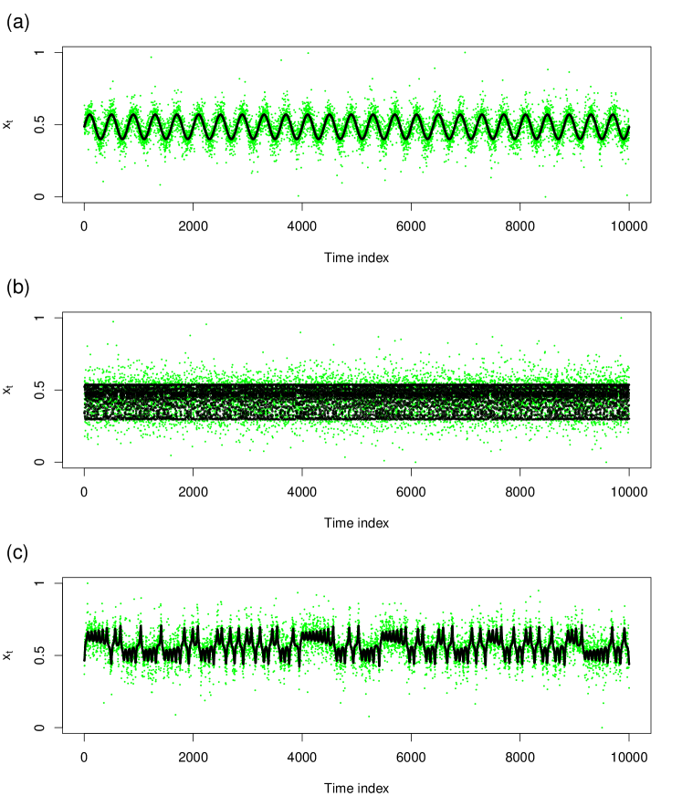
Figure 1: The examples of studied time series, (a) periodic function, (b) Logistic map, (c) Lorenz system, the green points denote the time series disturbed with white noise, the black points denote the time series without noise. Here the SNR is 1:1.

2 Recurrence quantification analysis

Recurrence quantification analysis (RQA) is a handy and versatile tool of nonlinear analysis, introduced in 1992 by Zbilut and Webber (1992) and extended by Marwan et al. (2002). RQA provides measures of complexity that evaluate the properties of the recurrence plot (RP), a graphical tool used for investigating the behaviour of state space trajectories $\vec{x}_{i}$Eckmann et al. (1987).

The basis of RQA is calculating the recurrence matrix

$$R_{i,j}=H(\varepsilon-\|\vec{x}_{i}-\vec{x}_{j}\|)\quad i,j=1,...,N,$$ (1)

where $N$ is the number of measured points $\vec{x}_{i}$, $\|\cdot\|$ is a norm which, in this work, is the maximum norm $\|\vec{x}\|_{\max}:=\max(|x_{1}|,\dots,|x_{n}|)$ for $\vec{x}\in\mathbb{R}^{n}$. $\varepsilon$ is a threshold distance, defining the recurrence of a state by its spatial closeness to a former state. The selection of $\varepsilon$ is crucial and depends on the specific research question and can have a strong effect on the result. $H(\cdot)$, is the Heaviside function, defined as

$$H(\varepsilon)=\begin{cases}1,&\varepsilon>0\\ 0,&\varepsilon\leq 0.\end{cases}$$ (2)

Eq. (1) results in a symmetrical square matrix that consists of binary values, i.e., zeros and ones. The RP is obtained as a plot of this square matrix.

There RQA measures we use in this work are

1. Recurrence rate (RR)

   $$RR=\frac{100}{N^{2}}\sum_{i,j=1}^{N}R_{i,j},$$ (3)

   which provides a measure for the density of recurrence points in the RP. Henceforth, we express this measure in percentages instead of decimals. $RR$ is directly related to the threshold $\varepsilon$ and is often used as the alternative way to preselect $\varepsilon$Kraemer et al. (2018).

2. Determinism (DET), quantifying how deterministic or well behaved a system is

   $$DET=\frac{\sum_{l=l_{\text{min}}}^{N}lP(l)}{\sum_{i,j=1}^{N}R_{i,j}},$$ (4)

   where $P(l)$ denotes the frequency distribution of the lengths $l$ of the diagonal lines and $l_{\min}$ denotes the minimal amount of points considered as line and it is set up to 2 as minimal value for all the calculations within this study.

Diagonal lines of the RP, parallel to the main diagonal point to the joint period when a trajectory accompanies locally close paths. Therefore, diagonal lines in the RP present the information of predictability and the deterministic content of the dynamical system. This property naturally suggest that the DET measure should be able to distinguish between signal of deterministic origin and stochastic noise.

3 Averaged RQA

As mentioned above, we consider a range of thresholds $\varepsilon$ to cover all scales in the variability of the time series. Instead of setting $\varepsilon$ to a certain value, we preselect $RR$ and use the corresponding value for $\varepsilon$Kraemer et al. (2018).

The novel approach here is to use averaged RQA quantities, which are calculated for a range of $RR$ values. For example, for the measure of determinism we define the averaged determinism

$$\overline{DET}_{RR_{*}}=\frac{1}{n}\sum_{RR=1}^{RR_{*}}DET_{RR},$$ (5)

where the $DET_{RR}$ denotes the $DET$ corresponding to a given value of the measure $RR$, $n$ is the number of considered $RR$ values for averaging, and $RR_{*}$ means the highest $RR$ to which is averaged and it can take any value from the interval $[0,\ldots,100]$. Naturally, the case $n=1$ cannot be seen as averaging and the case $RR_{*}=100$ should not be included, because the resulting RP does not contain any useful information about the dynamics. In this work we test the averaging for $RR_{*}\in[1,2,3,\dots,99]$.

Naturally, this approach can also be applied for other RQA measuresWebber and Marwan (2015) in order to catch their behaviour on more scales. This idea somehow resembles the concept of unthresholded recurrence plots discussed, e.g., by Iwanski and Bradley (1998), where instead of constructing a RP by thresholding the pairwise distances $\|\vec{x}_{i}-\vec{x}_{j}\|$ and representing the matrix by two colours, the entire distance matrix is represented, encoding the nonlinear properties of the system on all scales.

4 Methodology

The application of the above approach is used for discriminating different levels of noise from a deterministic signal. To illustrate this, we generate data with different fixed lengths, namely $10^{2},10^{3},10^{4},$ and $10^{5}$, where the number is in the sense of density of points, iteration, or integration time (divided by 100, because the step of 0.01) for periodic function, logistic map, and Lorenz system, respectively (details in Subsect. 4.1, 4.2, and 4.3). In order to investigate the quantitative information for every representative we generate 10 data sets of equidistantly different SNRs, where SNR is defined as the ratio between signal variance and noise variance.

We are studying the ability of sorting according to the various SNRs (definition below), expressing the ability to sort the 10 signals with different SNRs, while it is averaged for 10 realizations. In addition, we generate the equidistant SNR ratios in 3 intervals to inspect the boundaries of this approach, namely, $[0.01,0.02,\dots,0.1]$, $[0.1,0.2,\dots,1]$, and $[1,2,\dots,10]$, where for each SNR interval there are 10 equidistantly separated values denoted as “SNR L. 0.1”, “SNR L. 1”, and “SNR L. 10” respectively.

The lowest SNR in this work analysed is of the order of one hundred of signal to one, or another way expressed 1:100 (signal:noise) and the highest SNR in this set is of the ratio 10:1. Overall the testing has been done on 3,600 time series, what corresponds to: 3 types of dynamics (periodic, Logistic map, Lorenz system) $\times$ 3 SNR Levels (SNR L. = 0.1, 1, and 10) $\times$ 4 lengths ($10^{2},10^{3},10^{4},10^{5}$) $\times$ 10 generated time series corresponding to some SNR Level $\times$ 10 realizations.

As a measure evaluate the sorting of time series according to their deterministic content (estimated by $\overline{DET}_{RR_{*}}$ or $DET_{RR}$) we introduce the sorting rate $S$. The sorting rate is defined as the difference between the places in ordering of $n=10$ time series by a $\overline{DET}_{RR_{*}}$ or $DET_{RR}$ measure, expressed by vector $x$ and the vector of the defined positions $y$ in absolute value, summed and then expressed as percentage of successful sort. It can mathematically be expressed as

$$S=\frac{\sum_{i=1}^{10}\left(\sum_{j=1}^{10}|z_{j}-y_{j}|\right)_{i}-\sum_{i=1}^{10}\left(\sum_{j=1}^{10}|x_{j}-y_{j}|\right)_{i}}{\sum_{i=1}^{10}\left(\sum_{j=1}^{10}|z_{j}-y_{j}|\right)_{i}}$$ (6)

where $x_{j}$ is the $j$-th element of the vector $x$ for some $i$-th realization, denoting the SNR/position of time series according it’s $\overline{DET}_{RR_{*}}$ or $DET_{RR}$ measure, and $y_{j}$ is the element of the vector of $y$ of the SNRs/positions in the natural (sorted) way, i.e., $y=[1,2,3,4,5,6,7,8,9,10]$, and vector $z$ represents the reversed $y$ vector. The summation over index $i$ is in the sense of the repetition of the same experiment, or in other words for 10 realizations of corrupting the time series by white noise, for the sake of obtaining a stable result. The term $\sum_{i=1}^{10}(\sum_{j=1}^{10}|x_{j}-y_{j}|)_{i})$ can be seen as the departure from the best sorting, and $\sum_{i=1}^{10}(\sum_{j=1}^{10}|z_{j}-y_{j}|)_{i})$ takes naturally the value of 500 when $i,j=1,2,\dots,10$ and represents the worst possible scenario. In the following, $S$ is expressed as percentages instead of decimals. A value of 100% means a successful sorting, a value towards 0% means a complete failure of sorting.

4.1 Periodic time series

In order to simulate periodic signals we have used the R library RobPer Thieler et al. (2016) which has the function tsgen, originally made for simulating light curves. The function actually has 11 parameters and allows to simulate periodic signals, which mimic the data from observations thanks to the features, e.g., presence of outliers or gaps. We set up parameter of sampling to “equi” for equidistant sampling without gaps and the type of the periodic fluctuation to “sine”. The number of sampling cycles that is observed is set up to 25 (Fig. 1a).

4.2 Logistic map

The Logistic map is a classical example of a simple non-linear dynamical system exhibiting a variety of periodic and chaotic dynamics, given by the quadratic equation $x_{n+1}=rx_{n}(1-x_{n})$. For the initial value of the variable $x_{0}\in(0,1)$, the logistic map generates sequences of real numbers $x_{n}\in(0,1)$. The behaviour of the sequence $x_{n}$ depends on the parameter $r$. Roughly speaking, the behaviour on $r\in[r_{0},4]$ is chaotic, with some occasional “islands of regularity”. The transition between regular and chaotic behaviour happens for $r=r_{0}\approx 3.56995$. In this work we generate time series from the logistic map using $r=3.679$, where the band merging causes frequent laminar states Marwan et al. (2002) (Fig. 1b).

4.3 Lorenz system

The well-known Lorenz system is continuous nonlinear, non-periodic, three-dimensional, and deterministic. The famous attractor can can be reproduced by solving $\dot{x}=\sigma(y-x)$, $\dot{y}=x(\rho-z)$, and $\dot{z}=xy-\beta z)$, with $\sigma=10$, $\beta=8/3$, and $\rho=28$. The equations are integrated numerically with a Runge-Kutta solver and a time step 0.01. Finally, we use the $x$ value to emulate an observation by just one time series (Fig. 1c).

An essential step in nonlinear time series analysis is state space reconstruction. The dynamics of a $m$-dimensional nonlinear system can be reconstructed (in topological sense) from a single time series using the mathematical embedding theorem Takens (1981). The usual approach of state space reconstruction is delay coordinate embedding. The original scalar time series is mapped into a new space which is defined by the number of delayed dimensions $m$. The $m$-dimensional vector $\vec{x}(t)$ is constructed from $m$ samples of time series ${y}(t)$ using the delay $\tau$ by $\vec{x}(t)=[{y}(t),{y}(t-\tau),{y}(t-2\tau),\dots,{y}(t-(m-1)\tau)]$ In practice, when dealing with unknown systems, the values of $\tau$ and $m$ need to be estimated numericallyBradley and Kantz (2015); Cao (1997); Jiao et al. (2017). However, in the case of Lorenz system the dynamics is known and the parameters are set up to $\tau=3$ and $m=3$.

5 Technical implementation on a GPU

The measures of RQA are computationally expensive when computed naively because they are calculated from a RP, Eq. (1) that grows as $\mathcal{O}(N^{2})$, where $N$ is the length of the time series (or phase space vector) being analysed. More importantly, the memory footprint also grows as $\mathcal{O}(N^{2})$. Thus, even modestly sized time series will take a long time to be calculated on a standard system. Therefore, developing faster implementations and techniques to calculate RQA measures is crucial. Schultz et al. (2015) have shown that in the special case where the threshold is zero, some RQA measures can be obtained with $\mathcal{O}(N\log(N))$ complexity in $\mathcal{O}(N)$ space and have proposed approximations for RQA measures that have same computational complexity for thresholds above zero Schultz et al. (2015).

Calculating the RQA measures using a parallel approach where we can distribute the computational load to multiple processors/cores is equally important. GPUs are an ideal platform for RQA implementation as they possess a good combination of a large number of processing cores (NVIDIA A100 GPU has 6912 floating-point cores) and high bandwidth to memory (NVIDIA A100 has 1555GB/s). We have developed a parallel GPU accelerated software for NVIDIA GPUs written in CUDA. There are other packages which take advantage of parallelising calculations and GPU acceleration. For example, Rawald et al. (2017) have implemented RQA calculation using the OpenCL framework. We have designed the algorithms to have a minimal memory footprint ($\mathcal{O}(N)$) to allow performing RQA even on very long time series (100k+ points).

For most RQA measures, two types of tasks are required. First, counting the frequency of lines $l$ of a given length, producing a histogram of diagonal line lengths. The second is the density of the RP, which is used to calculate RR. However, RR can also be calculated from the histogram of line lengths. Thus, the histogram is used for the calculation of (DET, L, $\mathrm{L}_{\max}$ and RR). To calculate the histogram, we exploit the symmetric property of the $R_{i,j}$ matrix that allows us to use only the upper triangle of the $R_{i,j}$ matrix (i.e., $j>i$). We also calculate the value of the element $R_{i,j}$ on the fly, thus avoiding a significant memory footprint that would be otherwise required to store the whole $R_{i,j}$ matrix or any of its sub-matrices.

To calculate the histogram of line lengths, we use a stencil operation (a filter applied at every point of the RP) that flags the beginning and the end of each line. These flags are then aligned and compared, allowing us to calculate the length of all lines in a parallel implementation on multiple GPU workers.

6 Results

We focus on a comparison between the averaging approach and the approach of a fixed choice of some threshold value.

In Tab. 1 the sorting rates $S$ between the $\overline{DET}_{99}$ and the $DET_{1}$ are presented, what corresponds to the average of $DET$ for $RR\in[1,2,3,\dots,99][\%]$ and just for $RR=1[\%]$, respectively. Thus, $\overline{DET}_{99}$ is the universal choice which covers all the scales (except for RR=100%). $DET_{1}$ is selected for this comparison as the value of RR as recommended by Zbilut et al. (2002) for the construction of RPs. Here we find that the choice of $DET_{1}$ performs better only in few cases when the lengths and SNRs of the time series are lower (Tab. 1).

Next we consider the performance of the sorting using $\overline{DET}_{RR_{*}}$ for different values of $RR_{*}$ as the largest limit in Eq. (5) and for the single RR based $DET_{RR}$ (Figs. 2, 3 and 4). We find more robust results by the averaging approach $\overline{DET}_{RR_{*}}$ when compared to $DET_{RR}$.

For better understanding, the results from the first row in Tab. 1 are depicted in Fig. 2 as the first left-right pair from the top where the $y$-axis is denoted as “SNR L. $=0.1$”. The colours correspond to the considered time series length. Following this logic, the values 32 / 33.2 (Tab. 1) representing $S$ for the periodic functions with the level of $SNR\in[0.01,0.02,\dots,0.1]$ of the lengths 100 depicted in Fig. 2, are $\overline{DET}_{99}$, which is visible as the last point of the light brown line in the left plot and the $DET_{1}$ value, which naturally is to observe in both parts of the figure because of $\overline{DET}_{1}=DET_{1}$, as the average of one value is the value itself.

The most interesting feature of the comparison of the both approaches is the consistency of the averaging approach, for which the variability in $\overline{DET}_{RR_{*}}$ tends to be rather steady with low variance after some values of $RR$ (Figs. 2, 3 and 4, left panel), while for ${DET}_{RR}$ the ability to sort the data is in most of the cases not steady for neighbouring $RRs$ (Figs. 2, 3 and 4, right panel).

The simulations of the ability to sort data according their SNR measured with the sorting rate $S$ is in favour of the averaging approach, primarily in such sense, when we chose some RR value, the averaging up to that RR results in a more accurate and robust result. Although some exceptions can be found, the importance of the averaging is the consistency which is absent in the standard approach of choosing one fixed $RR$. This numerical simulation also shows that there is no universal, preferred threshold (or RR) value for which the best results can be achieved (Tab. 2, Fig. 5). Here we further average $\overline{DET}_{RR_{*}}$ over all considered lengths and SNRs (as shown in Figs. 2, 3, and 4) to provide an aggregated impression of the dependency of the accuracy with respect to the chosen maximal RR. We observe some trends, e.g., both approaches perform better for $RR>15\%$, which was not so obvious in Figs. 2, 3, and 4. On the other side of the sorting ability, the approach with single choice of RR is getting low for very high roughly $RR>60\%$ where the thresholds are too high to recognize the determinism, while this phenomenon is sometimes also present for the averaging approach but to much less extent.

We observe that the ability to sort the time series according their SNR is mostly ordered according the length of analysed time series (Fig. 2 to 4), the gap between the shortest time series and the rest is mostly visible by the averaging approach, while for the single choice approach there is often no such clear pattern to observe.

Table 1: Sorting rate $S$ for various time series, SNRs and time series lengths. The number left of the slash denotes $S$ of the averaging approach, when averaged to $RR_{*}=99\%$, the right sight the case for fixed $RR=1\%$.

type/length	100	1000	10000	100000
sin 0.1	32 / 33.2	40 / 36	40 / 40	60 / 20
sin 1	24 / 30.4	88 / 64	100 / 20	100 / 16
sin10	20 / 32	100 / 64	100 / 80	100 / 92
log 0.1	60 / 42.8	28 / 40	56 / 32	48 / 32
log 1	64 / 32.8	76 / 52	92 / 8	100 / 8
log10	76 / 32.4	100 / 56	100 / 60	100 / 76
lor 0.1	44 / 35.2	76 / 68	76 / 52	80 / 56
lor 1	68 / 36	96 / 68	100 / 84	100 / 84
lor 10	64 / 40.4	96 / 72	100 / 96	100 / 96

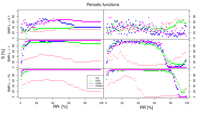
Figure 2: This plot shows the sorting rate $S$ of both averaging and classical approach of choosing $RR_{*}$ or $RR$ for the disturbed periodic functions.

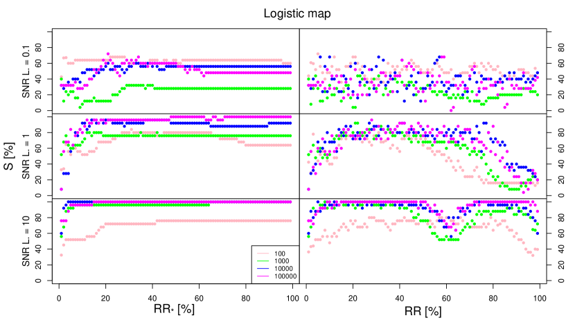
Figure 3: This plot shows the sorting rate $S$ of both averaging and classical approach of choosing $RR_{*}$ or $RR$ for the disturbed Logistic map.

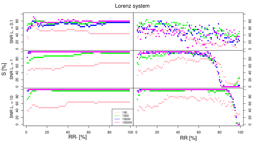
Figure 4: This plot shows the sorting rate $S$ of both averaging and classical approach of choosing $RR_{*}$ or $RR$ for the disturbed Lorenz system.

Table 2: This table shows the $RR_{*}$ or $RR$, for which the best sorting is achieved. The number to left of the slash denotes the $RR_{*}$ of the averaging approach for which the best sorting is achieved, the right sight the case for fixed $RR$, the numbers in parenthesis denote the amount of higher $RR_{*}$ or $RR$ for which the same sorting rate $S$ would be achieved.

type/length	100	1000	10000	100000
sin 0.1	45 (14) / 87 (1)	13 (40) / 95 (1)	28 (2) / 28 (1)	24 (2) / 4 (3)
sin 1	23 (8) / 18 (1)	39 (21) / 29 (3)	13 (58) / 10 (6)	10 (90) / 38 (6)
sin10	29 (7) / 25 (1)	10 (90) / 9 (34)	4 (96) / 7 (68)	3 (97) / 6 (75)
log 0.1	22 (7) / 5 (1)	1 (1) / 4 (5)	21 (7) / 6 (4)	21 (1) / 58 (2)
log 1	31 (1) / 16 (1)	12 (8) / 21 (2)	14 (17) / 27 (5)	48 (46) / 28 (1)
log10	42 (58) / 27 (10)	65 (35) / 8 (11)	4 (96) / 5 (30)	15 (85) / 9 (63)
lor 0.1	8 (2) / 3 (1)	9 (1) / 10 (1)	6 (2) / 21 (3)	7 (1) / 29 (1)
lor 1	70 (30) / 40 (4)	65 (7) / 29 (12)	3 (97) / 10 (31)	2 (96) / 4 (45)
lor 10	40 (57) / 30 (2)	10 (15) / 4 (28)	3 (97) / 3 (85)	2 (98) / 3 (83)

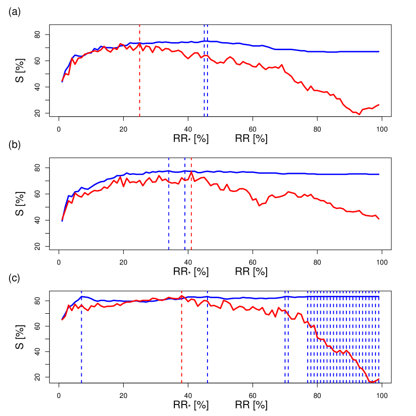
Figure 5: Averaged sorting rate $S$ of the averaging approach (blue line) and fixed threshold approach (red line). The dashed vertical lines denote the position of the maximum. The presented $S$ are averages over all lengths and SNR levels for (a) periodic functions, (b) logistic map, and (c) Lorenz system respectively. The labels on y-axis denotes both approaches, averaging and fixed one respectively. We observe that for most of the $RR_{*}$ and $RR$ values, the blue line is above the red line, representing better sorting performance of the average determinism.

7 Discussion

In this study we have proposed a novel approach for performing a threshold free RQA and demonstrated its performance. The selection of the threshold can be avoided by averaging the RQA measure of interest which was calculated for a range of thresholds. We tested the ability of sorting data sets corrupted by white noise according their signal to noise ratios with the help of averaged DET measure. The new approach performs more robust than standard single threshold approach. The explanation of the results is that the deterministic behaviour can be detected on more scales and provides a more robust RQA DET measure.

This property has been also achieved when time series embedding is applied, as for the Lorenz system, where the embedding parameters have been set to 3 for the time lag as for the embedding dimension.

For the purpose of identifying deterministic components in noisy signals, the proposed approach might be the practical choice. The found RR value, out of this analysis, up to which the averaging should be performed is $RR_{*}\approx 40\%$, as in the vicinity of this value the maxima of the sorting rates were achieved for all the systems (Fig. 5). It also corresponds to previous findings that the discrimination of deterministic signals from noise works well for a quite large range of thresholds $\varepsilon$Schinkel et al. (2008). Averaging to larger $RR_{*}$ might also work, but could reduce the robustness of the RQA measures.

However, we are aware of the fact that the complexity of the analysed artificial data is limited, and in the future further features could be introduced in order to explore the boundaries of this approach, namely gaps, other types of noise, different lengths of time series and sampling. The latter factors would help to better mimic the data obtained from unknown systems as they are the typical challenges in data analysis. Moreover, the suggested averaging approach was developed for the research question on discrimination a signal component from noisy signals, in particular, to order them with respect to the SNR. Whether it works also for other purpose should be studied in more detail in the future.

References

- Bradley and Kantz [2015] Elizabeth Bradley and Holger Kantz. Nonlinear time-series analysis revisited. Chaos, 25(9):097610, September 2015. doi: 10.1063/1.4917289.
- Webber and Marwan [2015] Jr. Webber, Charles L. and Norbert Marwan. Recurrence Quantification Analysis. Springer, 2015.
- Marwan [2011] N. Marwan. How to avoid potential pitfalls in recurrence plot based data analysis. International Journal of Bifurcation and Chaos, 21(4):1003–1017, 2011. doi: 10.1142/S0218127411029008.
- Thiel et al. [2002] Marco Thiel, M. Carmen Romano, Jürgen Kurths, Riccardo Meucci, Enrico Allaria, and F. Tito Arecchi. Influence of observational noise on the recurrence quantification analysis. Physica D Nonlinear Phenomena, 171(3):138–152, October 2002. doi: 10.1016/S0167-2789(02)00586-9.
- Medrano et al. [2021] Johan Medrano, Abderrahmane Kheddar, Annick Lesne, and Sofiane Ramdani. Radius selection using kernel density estimation for the computation of nonlinear measures. Chaos, 31(8):083131, August 2021. doi: 10.1063/5.0055797.
- Andreadis et al. [2020] Ioannis Andreadis, Athanasios D. Fragkou, and Theodoros E. Karakasidis. On a topological criterion to select a recurrence threshold. Chaos, 30(1):013124, January 2020. doi: 10.1063/1.5116766.
- Schinkel et al. [2008] S. Schinkel, O. Dimigen, and N. Marwan. Selection of recurrence threshold for signal detection. European Physical Journal Special Topics, 164(1):45–53, October 2008. doi: 10.1140/epjst/e2008-00833-5.
- Cencini et al. [2000] M. Cencini, M. Falcioni, E. Olbrich, H. Kantz, and A. Vulpiani. Chaos or noise: Difficulties of a distinction. Physical Review E, 62(1):427–437, July 2000. doi: 10.1103/PhysRevE.62.427.
- Urry [1996] C. M. Urry. An Overview of Blazar Variability. In H. Richard Miller, James R. Webb, and John C. Noble, editors, Blazar Continuum Variability, volume 110 of Astronomical Society of the Pacific Conference Series, page 391, January 1996.
- Mohorian et al. [2021] Maksym Mohorian, Gopal Bhatta, Tek P Adhikari, Niraj Dhital, Radim Pánis, Adithiya Dinesh, Suvas C Chaudhary, Rajesh K Bachchan, and Zdeněk Stuchlík. X-ray timing and spectral variability properties of blazars s5 0716 + 714, OJ 287, mrk 501, and RBS 2070. Monthly Notices of the Royal Astronomical Society, 510(4):5280–5301, dec 2021. doi: 10.1093/mnras/stab3738.
- Mayer et al. [2010] L. Mayer, S. Kazantzidis, A. Escala, and S. Callegari. Direct formation of supermassive black holes via multi-scale gas inflows in galaxy mergers. Nature, 466(7310):1082–1084, aug 2010. ISSN 0028-0836. doi: 10.1038/nature09294.
- Francis et al. [1991] Paul J. Francis, Paul C. Hewett, Craig B. Foltz, Frederic H. Chaffee, Ray J. Weymann, and Simon L. Morris. A High Signal-to-Noise Ratio Composite Quasar Spectrum. Astrophysical Journal, 373:465, June 1991. doi: 10.1086/170066.
- Thorne [1995] K. S. Thorne. Gravitational Waves. In E. W. Kolb and R. D. Peccei, editors, Particle and Nuclear Astrophysics and Cosmology in the Next Millenium, page 160, January 1995.
- Marwan et al. [2002] Norbert Marwan, Niels Wessel, Udo Meyerfeldt, Alexander Schirdewan, and Jürgen Kurths. Recurrence-plot-based measures of complexity and their application to heart-rate-variability data. Physical Review E, 66(2):026702, August 2002. doi: 10.1103/PhysRevE.66.026702.
- Kraemer et al. [2021] K. H. Kraemer, G. Datseris, J. Kurths, I. Z. Kiss, J. L. Ocampo-Espindola, and N. Marwan. A unified and automated approach to attractor reconstruction. New Journal of Physics, 23:033017, 2021. doi: 10.1088/1367-2630/abe336.
- Zbilut and Webber [1992] Joseph P. Zbilut and Charles L. Webber. Embeddings and delays as derived from quantification of recurrence plots. Physics Letters A, 171(3-4):199–203, December 1992. doi: 10.1016/0375-9601(92)90426-M.
- Eckmann et al. [1987] J. P. Eckmann, S. Oliffson Kamphorst, and D. Ruelle. Recurrence plots of dynamical systems. EPL (Europhysics Letters), 4:973, November 1987. doi: 10.1209/0295-5075/4/9/004.
- Kraemer et al. [2018] K. H. Kraemer, R. V. Donner, J. Heitzig, and N. Marwan. Recurrence threshold selection for obtaining robust recurrence characteristics in different embedding dimensions. Chaos, 28(8):085720, 2018. doi: 10.1063/1.5024914.
- Iwanski and Bradley [1998] Joseph S. Iwanski and Elizabeth Bradley. Recurrence plots of experimental data: To embed or not to embed? Chaos, 8(4):861–871, December 1998. doi: 10.1063/1.166372.
- Thieler et al. [2016] Anita M. Thieler, Roland Fried, and Jonathan Rathjens. RobPer: An R Package to Calculate Periodograms for Light Curves Based on Robust Regression. Journal of Statistical Software, 69(9):1–36, 2016. doi: 10.18637/jss.v069.i09.
- Takens [1981] Floris Takens. Detecting strange attractors in turbulence. In Lecture Notes in Mathematics, Berlin Springer Verlag, volume 898, page 366. 1981. doi: 10.1007/BFb0091924.
- Cao [1997] Liangyue Cao. Practical method for determining the minimum embedding dimension of a scalar time series. Physica D Nonlinear Phenomena, 110(1):43–50, February 1997. doi: 10.1016/S0167-2789(97)00118-8.
- Jiao et al. [2017] Jiantao Jiao, Kartik Venkat, and Tsachy Weissman. Mutual Information, Relative Entropy and Estimation Error in Semi-martingale Channels. arXiv e-prints, art. arXiv:1704.05199, April 2017.
- Schultz et al. [2015] David Schultz, Stephan Spiegel, Norbert Marwan, and Sahin Albayrak. Approximation of diagonal line based measures in recurrence quantification analysis. Physics Letters A, 379, 02 2015. doi: 10.1016/j.physleta.2015.01.033.
- Rawald et al. [2017] Tobias Rawald, Mike Sips, and Norbert Marwan. Pyrqa - conducting recurrence quantification analysis on very long time series efficiently. Comput. Geosci., 104:101–108, 2017.
- Zbilut et al. [2002] Joseph P. Zbilut, José-Manuel Zaldivar-Comenges, and Fernanda Strozzi. Recurrence quantification based Liapunov exponents for monitoring divergence in experimental data. Physics Letters A, 297(3-4):173–181, May 2002. doi: 10.1016/S0375-9601(02)00436-X.