Modified Unscented Kalman Filter

Two Modifications of the Unscented Kalman Filter that
Specialize to the Kalman Filter for Linear Systems

On the Accuracy of the One-step UKF and the Two-step UKF

Abstract

The most accurate version of the unscented Kalman filter (UKF) involves the construction of two ensembles. To reduce computational cost, however, UKF is often implemented without the second ensemble. This simplification comes at a price, however, since, for linear systems, the one-step variation of the two-step UKF does not specialize to the classical Kalman filter, with an associated loss of accuracy. This paper remedies this drawback by developing a modified one-step UKF that recovers the classical Kalman filter for linear systems. Numerical examples show that the modified one-step UKF also recovers the accuracy of the two-step UKF in nonlinear systems with linear outputs.

I Introduction

The Unscented Kalman filter (UKF) is widely applied to nonlinear estimation problems [1]. UKF was introduced in [2, 3] has been applied to a wide array of engineering and scientific applications including attitude estimation [4], navigation [5], battery-charge estimation [6], and state and parameter estimation in atmospheric models [7].

Like the Ensemble Kalman filter (EnKF) [8], UKF propagates an ensemble in order to compute the mean and covariance of the state estimate. However, unlike EnKF, which approximates the covariance using statistics of the propagated ensembles, UKF uses unscented transformations to approximate the covariances, which allows UKF to reduce the size of the ensemble to $2n+1,$ where $n$ is the dimension of the state of the system [9]. Since UKF propagates the ensemble using the nonlinear dynamics map, the accuracy of UKF is expected and is also reported to be better than that of the Extended Kalman filter, which is based on the linearized dynamics [10].

The classical UKF requires generation of a $2n+1$ size ensemble twice at every step[1, p. 447], [11, p. 86]. The first ensemble is used to propagate the estimated state and compute the prior covariance, whereas the second ensemble is used to approximate cross-covariance matrices needed to compute the filter gain. This is the two-step UKF. Since the UKF gain and covariance update are motivated by the corresponding expressions used in the Kalman filter, it is reasonable to expect that, in the case of a linear system, the UKF gain and the covariance update will coincide with Kalman filter. As expected, the two-step UKF indeed specializes to the classical Kalman filter when applied to a linear system, as explicitly shown in Section III.

In the two-step UKF, the prior estimate and the prior covariance computed after propagating the first ensemble through the dynamics of the system are used to generate the second ensemble, which is then further transformed into the output ensemble using the algebraic output equation. In order to reduce implementation complexity and reduce computational cost, second ensemble generation is often omitted. Instead, the propagated ensemble is used for further computations. This is the one-step UKF. In fact, the UKF originally introduced in [9, 2, 3] presented the one-step formulation. However, it turns out that, the one-step UKF does not specialize to the classical Kalman filter when applied to a linear system. This is due to the fact that effect of the process noise does not pass through to the output-error covariance. In fact, one-step UKF output covariances and the propagated state covariance are found to be missing the process noise term when applied to a linear system, as shown in this paper.

This paper presents a modification of the one-step UKF that recovers the accuracy of the two-step UKF for systems where the output equation is linear with only one ensemble generation. Like the two-step UKF, the one-step modified UKF (MUKF) specializes to the Kalman filter for linear systems. In particular, we show explicitly that the two-step UKF specializes to the the Kalman filter in the case of a linear system. Next, we show that the accuracy of the one-step UKF is worse than the accuracy of the two-step UKF in the case of linear system by explicitly stating the missing terms. Finally, by including the missing terms, we present the one-step modified UKF that recovers the accuracy of the two-step UKF.

This paper is organized as follows. Section II briefly reviews the Kalman filter to introduce the terminology and notation used in this paper. Section III briefly reviews the two-step UKF and shows that, for linear systems, it specializes to the classical Kalman filter. Section IV reviews the one-step UKF to a linear system and shows that, for linear systems, it does not specialize to the classical Kalman filter. Section V presents a modification of the one-step UKF that specializes to the classical Kalman filter in the case of linear systems. Section VI applies the proposed extension to two nonlinear systems and compares the accuracy of uncertainty propagation. Finally, the paper concludes with a discussion in Section VII.

II Summary of the Kalman Filter

This section briefly reviews the Kalman filter to introduce terminology and notation for later sections. Consider a linear system

$$x_{k+1} =A_{k}x_{k}+B_{k}u_{k}+w_{k},$$ (1)

$$y_{k} =C_{k}x_{k}+v_{k},$$ (2)

where, for all $k\geq 0$, $A_{k},B_{k},C_{k}$ are real matrices, $w_{k}\sim{\mathcal{N}}(0,Q_{k})$ is the disturbance, and $v_{k}\sim{\mathcal{N}}(0,R_{k})$ is the sensor noise.

For the system (1), (2), the Kalman filter is

$$\hat{x}_{k+1|k} =A_{k}\hat{x}_{k|k}+B_{k}u_{k},$$ (3)

$$\hat{x}_{k+1|k+1} =\hat{x}_{k+1|k}+K_{k+1}(y_{k+1}-C_{k+1}\hat{x}_{k+1|k}),$$ (4)

where $\hat{x}_{k+1|k}$ is the prior estimate, $\hat{x}_{k+1|k+1}$ is the posterior estimate at step $k+1,$ and the Kalman gain $K_{k+1}$ is given by

$$K_{k+1} =P_{k+1|k}C_{k+1}^{\rm T}\overline{R}_{k+1}^{-1}.$$ (5)

The prior covariance $P_{k+1|k}$ at step $k+1$ is given by

$$P_{k+1|k} =A_{k}P_{k|k}A_{k}^{\rm T}+Q_{k},$$ (6)

and the posterior covariance at step $k+1$ is given by

$$P_{k+1|k+1}=P_{k+1|k}-P_{k+1|k}C_{k+1}^{\rm T}\overline{R}_{k+1}^{-1}C_{k+1}P_{k+1|k}.$$ (7)

where

$$\overline{R}_{k+1}\stackrel{{\scriptstyle\triangle}}{{=}}C_{k+1}P_{k+1|k}C_{k+1}^{\rm T}+R_{k+1}.$$ (8)

The Kalman filter is (3), (4) where $K_{k+1}$ is given by (5) and the covariance matrices are updated by (6), (7).

Next, in order to establish connections with UKF, (5), (7) are reformulated in terms of covariance matrices instead of $A_{k}$ and $C_{k+1}$. Defining

$$P_{z_{k+1|k+1}} \stackrel{{\scriptstyle\triangle}}{{=}}C_{k+1}P_{k+1|k}C_{k+1}^{\rm T}+R_{k+1},$$ (9)

$$P_{e,z_{k+1|k}} \stackrel{{\scriptstyle\triangle}}{{=}}P_{k+1|k}C_{k+1}^{\rm T},$$ (10)

and substituting (9) and (10) in (5) and (7), the Kalman gain can be written as

$$K_{k+1} =P_{e,z_{k+1|k}}P_{z_{k+1|k+1}}^{-1},$$ (11)

and the corresponding optimized posterior covariance at step $k+1$ can be written as

$$P_{k+1|k+1} =P_{k+1|k}-K_{k+1}P_{e,z_{k+1|k}}^{\rm T}.$$ (12)

As shown in the next section, UKF approximates the covariance matrices $P_{k+1|k},$ $P_{z_{k+1|k+1}},$ and $P_{e,z_{k+1|k}}$ by using ensembles instead of $A_{k}$ and $C_{k+1}.$

III Summary of Two-Step UKF

This section briefly reviews the classical two-step unscented Kalman filter to establish notation and terminology for use in the rest of the paper. The UKF algorithm is formulated using a compact matrix-based notation and is based on the algorithm presented in [11, p. 86].

Consider a system

$$x_{k+1} =f_{k}(x_{k},u_{k})+w_{k},$$ (13)

$$y_{k} =g_{k}(x_{k})+v_{k},$$ (14)

where, for all $k\geq 0$, $f_{k},g_{k},C_{k}$ are real-valued vector functions, $w_{k}\sim{\mathcal{N}}(0,Q_{k})$ is the disturbance, and $v_{k}\sim{\mathcal{N}}(0,R_{k})$ is the sensor noise.

The following notation is used to present ensembles in a compact manner. Let $x\in{\mathbb{R}}^{l_{x}}$ and $P\in{\mathbb{R}}^{l_{x}\times l_{x}}$ be positive definite. The ensemble $X(x,P)\in{\mathbb{R}}^{l_{x}\times(2l_{x}+1)}$ is the matrix

$$X(x,P)\stackrel{{\scriptstyle\triangle}}{{=}}[x\ x+p_{1}\ \cdots\ x+p_{l_{x}}\ x-p_{1}\ \cdots\ x-p_{l_{x}}],$$

where $p_{i}$ is the $i$-th column of $P.$ Let $\alpha>0.$ Define

$$W\stackrel{{\scriptstyle\triangle}}{{=}}\dfrac{1}{2\alpha^{2}l_{x}}\begin{bmatrix}2(\alpha^{2}-1)l_{x}\\ 1_{2l_{x}\times 1}\\ \end{bmatrix}\in{\mathbb{R}}^{2l_{x}+1}.$$

The weighted mean of the ensemble $X$ is $\bar{x}\stackrel{{\scriptstyle\triangle}}{{=}}XW,$ and the ensemble perturbation is $\tilde{X}\stackrel{{\scriptstyle\triangle}}{{=}}X-H(\bar{x}),$ where, for $v\in{\mathbb{R}}^{n},$ $H(v)\stackrel{{\scriptstyle\triangle}}{{=}}1_{1\times 2l_{x}+1}\otimes v\in{\mathbb{R}}^{n\times(2l_{x}+1)}.$ Note that $\otimes$ is the Kronecker product [12].

In order to compute the filter gain $K_{k+1}$ and the posterior covariance $P_{k+1|k+1},$ UKF approximates the covariance matrices $P_{k+1|k},$ $P_{z_{k+1|k+1}},$ and $P_{e,z_{k+1|k}}$ in (11) and (12) by propagating an ensemble of $2l_{x}+1$ sigma points.

For all $k\geq 0$, the $i$-th sigma point $\hat{x}_{\sigma_{i},k}$ is defined as the $i$-th column of

$$X_{k|k}\stackrel{{\scriptstyle\triangle}}{{=}}X\left(\hat{x}_{k|k},\alpha\sqrt{l_{x}P_{k|k}}\right),$$ (15)

where $\alpha\in{\mathbb{R}}$ is a tuning parameter and $P_{k|k}$ is the posterior covariance given by UKF at step $k$. Then, for $i=1,\ldots,2l_{x}+1,$ the sigma points are propagated as

$$\hat{x}_{\sigma_{i},k+1} =f_{k}(\hat{x}_{\sigma_{i},k},u_{k}).$$ (16)

The prior estimate and the prior covariance at step $k+1$ are given by

$$\hat{x}_{k+1|k} =X_{k+1|k}W,$$ (17)

$$P_{k+1|k} =\tilde{X}_{k+1|k}W_{\rm d}\tilde{X}_{k+1|k}^{\rm T}+Q_{k},$$ (18)

where

$$X_{k+1|k} \stackrel{{\scriptstyle\triangle}}{{=}}\begin{bmatrix}\hat{x}_{\sigma_{1},k+1}&\cdots&\hat{x}_{\sigma_{2l_{x}+1},k+1}\end{bmatrix}.$$ (19)

Next, the posterior estimate and the posterior covariance at step $k+1$ are computed by regenerating sigma points as shown next. Defining

$$X_{k+1|k}^{\prime}\stackrel{{\scriptstyle\triangle}}{{=}}X\left(\hat{x}_{k+1|k},\alpha\sqrt{l_{x}P_{k+1|k}}\right),$$ (20)

the output of the $i$-th sigma point is given by

$$\hat{y}_{\sigma_{i},k+1} =g_{k+1}(X_{k+1|k}^{\prime}e_{i}),$$ (21)

where $e_{i}$ is the $i$-th column of $I_{2l_{x}+1}.$ The covariance matrices $P_{z_{k+1|k+1}}$ and $P_{e,z{k+1|k}}$ are then given by

$$P_{z_{k+1|k+1}} =\tilde{Y}_{k+1}W_{\rm d}\tilde{Y}_{k+1}^{\rm T}+R_{k+1},$$ (22)

$$P_{e,z_{k+1|k}} =\tilde{X}_{k+1|k}^{\prime}W_{\rm d}\tilde{Y}_{k+1}^{\rm T},$$ (23)

where

$$Y_{k+1}\stackrel{{\scriptstyle\triangle}}{{=}}\begin{bmatrix}\hat{y}_{\sigma_{1},k+1}&\cdots&\hat{y}_{\sigma_{2l_{x}+1},k+1}\end{bmatrix}\in{\mathbb{R}}^{l_{y}\times 2l_{x}+1}.$$ (24)

Finally, the posterior estimate at step $k+1$ is

$$\hat{x}_{k+1|k+1} =\hat{x}_{k+1|k}+K_{k+1}(y_{k+1}-Y_{k+1}W),$$ (25)

and the posterior covariance at step $k+1$ is

$$P_{k+1|k+1} =P_{k+1|k}-K_{k+1}P_{e,z_{k+1|k}}^{{\rm T}},$$ (26)

where

$$K_{k+1} =P_{e,z_{k+1|k}}P_{z_{k+1|k+1}}^{-1}.$$ (27)

The two-step UKF is (17), (25) where the posterior covariance is given by (26) and the filter gain is given by (27). Note that (26), (27) are similar to and are in fact motivated by (11), (12). The various covariance matrices computed in the two-step UKF are summarized in Table I.

Variable	Two-step UKF	One-step UKF	Modified One-step UKF
$X_{k|k}$	$X(\hat{x}_{k|k},\alpha\sqrt{P_{k|k}})$	$X(\hat{x}_{k|k},\alpha\sqrt{P_{k|k}})$	$X(\hat{x}_{k|k},\alpha\sqrt{P_{k|k}})$
	(15)	(15)	(15)
$P_{k+1|k}$	$\tilde{X}_{k+1|k}W_{\rm d}\tilde{X}_{k+1|k}^{\rm T}+Q_{k}$	$\tilde{X}_{k+1|k}W_{\rm d}\tilde{X}_{k+1|k}^{\rm T}+Q_{k}$	$\tilde{X}_{k+1|k}W_{\rm d}\tilde{X}_{k+1|k}^{\rm T}+Q_{k}$
	(18)	(18)	(18)
$X_{k+1|k}^{\prime}$	$X(\hat{x}_{k+1|k},\alpha\sqrt{P_{k+1|k}})$	$X_{k+1|k}$	$X_{k+1|k}$
	(20)	(19)	(19)
$P_{z_{k+1|k+1}}$	$\tilde{Y}_{k+1}W_{\rm d}\tilde{Y}_{k+1}^{\rm T}$	$\tilde{Y}_{k+1}W_{\rm d}\tilde{Y}_{k+1}^{\rm T}$	$\tilde{Y}_{k+1}W_{\rm d}\tilde{Y}_{k+1}^{\rm T}+Q_{k}C_{k+1}^{\rm T}$
	(22)	(34)	(42)
$P_{ez,_{k+1|k}}$	$\tilde{X}_{k+1|k}^{\prime}W_{\rm d}\tilde{Y}_{k+1}^{\rm T}+R_{k+1}$	$\tilde{X}_{k+1|k}W_{\rm d}\tilde{Y}_{k+1}^{\rm T}+R_{k+1}$	$\tilde{X}_{k+1|k}W_{\rm d}\tilde{Y}_{k+1}^{\rm T}+C_{k+1}Q_{k}C_{k+1}^{\rm T}+R_{k+1}$
	(23)	(35)	(43)

TABLE I: Ensembles and covariance matrices used in the two-step UKF, the one-step UKF, and the modified one-step UKF.

The following result shows that the two-step UKF specializes to the Kalman filter when applied to a linear system.

Proposition III.1

Consider the linear system (1), (2). Let $P_{k|k}$ be the posterior covariance given by the Kalman filter and let $P_{k|k}^{\rm UKF}$ be the posterior covariance given by the two-step UKF. Let $\hat{x}\in{\mathbb{R}}^{n}$ and let $P$ be positive definite. Assume that $\hat{x}_{k|k}^{\rm UKF}=\hat{x}_{k|k}^{\rm KF}=\hat{x}$ and $P_{k|k}^{\rm UKF}=P_{k|k}^{\rm KF}=P.$ Then,

$$P_{z_{k+1|k+1}}^{UKF} =P_{e,z_{k+1|k}}^{KF},$$ (28)

$$P_{e,z_{k+1|k}}^{UKF} =P_{e,z_{k+1|k}}^{KF}.$$ (29)

Furthermore,

$$\hat{x}_{k+1|k+1}^{\rm UKF} =\hat{x}_{k+1|k+1}^{\rm KF},$$ (30)

$$K_{k+1}^{\rm UKF} =K_{k+1},$$ (31)

$$P_{k+1|k+1}^{\rm UKF} =P_{k+1|k+1}^{\rm KF}.$$ (32)

Proof:

See Appendix VIII-A. ∎

Proposition III.1 implies that, in a linear system, the two-step UKF reduces to the Kalman filter. Furthermore, note that, in linear systems, the choice of $\alpha$ does not affect $K_{k+1}^{\rm UKF}$ and $P_{k+1|k+1}^{\rm UKF}.$

IV One-Step UKF

This section reviews the one-step UKF presented in [9, 2, 3, 1], where the second ensemble generation step, given by (20), is omitted in order to reduce computational effort and cost.

In this case, the output of the $i$-th sigma point is given by

$$\hat{y}_{\sigma_{i},k+1} =g_{k+1}(X_{k+1|k}e_{i}),$$ (33)

which uses the propagated ensemble $X_{k+1|k}$ given by (19), instead of regenerating a new ensemble using the prior estimate and the prior covariance. In the one-step UKF, the covariance matrices $P_{z_{k+1|k+1}}$ and $P_{e,z{k+1|k}}$ are given by

$$P_{z_{k+1|k+1}} =\tilde{Y}_{k+1}W_{\rm d}\tilde{Y}_{k+1}^{\rm T}+R_{k+1},$$ (34)

$$P_{e,z_{k+1|k}} =\tilde{X}_{k+1|k}W_{\rm d}\tilde{Y}_{k+1}^{\rm T}.$$ (35)

Note that (34) and (35) use the propagated ensemble $X_{k+1|k}$ to compute the perturbed ensembles instead of using the regenerated ensemble $X_{k+1|k}^{\prime}.$

The one-step UKF is (17), (25) where the posterior covariance is given by (26) and the filter gain is given by (27), However $P_{z_{k+1|k+1}}$ and $P_{e,z_{k+1|k}}$ used in (26), (27) are now given by (34), (35). The various covariance matrices computed in the one-step UKF are summarized in Table I.

The following result shows that the one-step UKF does not specialize to the Kalman filter when applied to a linear system.

Proposition IV.1

Consider the linear system (1), (2). Let $P_{k|k}$ be the posterior covariance given by the Kalman filter and let $P_{k|k}^{\rm UKF1}$ be the posterior covariance given by the one-step UKF. Let $\hat{x}\in{\mathbb{R}}^{n}$ and let $P$ be positive definite. Assume that $\hat{x}_{k|k}^{\rm UKF1}=\hat{x}_{k|k}^{\rm KF}=\hat{x}$ and $P_{k|k}^{\rm UKF1}=P_{k|k}^{\rm KF}=P.$ Then,

$$P_{z_{k+1|k+1}}^{UKF1} =P_{e,z_{k+1|k}}^{KF}-C_{k+1}Q_{k}C_{k+1}^{\rm T},$$ (36)

$$P_{e,z_{k+1|k}}^{UKF1} =P_{e,z_{k+1|k}}^{KF}-Q_{k}C_{k+1}^{\rm T},$$ (37)

Furthermore, assume that $Q_{k}\neq 0,$ and $C_{k}\notin{\mathcal{N}}(Q_{k}).$ Then,

$$\hat{x}_{k+1|k+1}^{\rm UKF1} \neq\hat{x}_{k+1|k+1}^{\rm KF},$$ (38)

$$K_{k+1}^{\rm UKF1} \neq K_{k+1},$$ (39)

$$P_{k+1|k+1}^{\rm UKF1} \neq P_{k+1|k+1}^{\rm KF},$$ (40)

$${\rm tr}\,(P_{k+1|k+1}^{\rm UKF1}) \leq{\rm tr}\,(P_{k+1|k+1}^{\rm KF}).$$ (41)

Proof:

See Appendix VIII-B. ∎

Proposition IV.1 implies that, in a linear system where disturbance is not zero, the one-step UKF does not reduce to the Kalman filter. That is, the posterior covariance propagated by the one-step UKF is not equal to the covariance given by (7). This inequality arises due to the fact that the output error covariance $P_{z_{k+1|k+1}}$ is missing the term $C_{k+1}Q_{k}C_{k+1}^{\rm T}$ and the cross-covariance $P_{e,z_{k+1|k}}$ is missing the term $Q_{k}C_{k+1}^{\rm T}.$ The next section presents a modification of the one-step UKF that includes the missing term and is thus more accurate than the one-step UKF. This modification is expecially beneficial for high-dimension nonlinear systems where the second sigma-point generation step adds considerable computational cost. Furthermore, the second sigma-point generation step makes the algorithm non-modular.

V One-Step Modified UKF

As shown in the previous section, the covariances $P_{z_{k+1|k+1}}$ and $P_{e,z_{k+1|k}}$ in (58) and (59) are missing terms that depend on the disturbance statistics $Q_{k}$, thus preventing one-step UKF from specializing to the Kalman filter for linear systems. To remedy this omission, this section presents the one-step modified UKF (MUKF), which specialize to the Kalman filter for linear systems. In this modification, the UKF covariance matrices (34), (35) are modified such that they specialize to (9), (10) in the case of linear systems.

Using the output matrix, MUKF adds the missing terms to $P_{z_{k+1|k+1}}$ and $P_{e,z_{k+1|k}}$. In particular, in MUKF, the covariance matrices $P_{z_{k+1|k+1}}$ and $P_{e,z{k+1|k}}$ are given by

$$P_{z_{k+1|k+1}} =\tilde{Y}_{k+1}W_{\rm d}\tilde{Y}_{k+1}^{\rm T}+C_{k+1}Q_{k}C_{k+1}^{\rm T}+R_{k+1},$$ (42)

$$P_{e,z_{k+1|k}} =\tilde{X}_{k+1|k}W_{\rm d}\tilde{Y}_{k+1}^{\rm T}+Q_{k}C_{k+1}^{\rm T}.$$ (43)

Note that, in the case of nonlinear systems, $C_{k+1}$ can be computed using the Jacobian of the output map.

Since, in the case of linear systems, the intermediate covariance matrices in MUKF include the missing terms, the one-step modified UKF recovers the accuracy of the classical two-step UKF. The next section applies the MUKF to two nonlinear systems to demonstrate this fact.

VI Numerical Examples

In this section, the two-step UKF, one-step UKF, and the one-step MUKF are applied to two nonlinear systems, namely, the Van der Pol Oscillator and the chaotic Lorenz system to demonstrate the erroneous covariance update in the one-step UKF and the recovery of the correct covariance update in the one-step MUKF.

Example VI.1

Van der Pol Oscillator. Consider the discretized Van der Pol Oscillator.

$$x_{k+1} =f(x_{k})+w_{k},$$ (44)

where

$$f(x)=\begin{bmatrix}x_{1}+T_{\rm s}x_{2}\\ x_{2}+T_{\rm s}(\mu(1-x_{1}^{2})x_{2}-x_{1})\end{bmatrix},$$ (45)

and $\mu=1.2.$ Let the measurement be given by

$$y_{k}=Cx_{k}+v_{k},$$ (46)

where $C\stackrel{{\scriptstyle\triangle}}{{=}}[1\ 0].$ For all $k\geq 0,$ let $Q_{k}=0.01I_{2}$ and $R_{k}=10^{-4}.$ Furthermore, let $x(0)=[1\ 1]^{\rm T}$ and $P_{0|0}=I_{3}$.

Letting $\alpha=1.5$ in the two-step UKF, the one-step UKF, and the one-step MUKF, Figure 1 shows the trace of the posterior covariance computed by the three filters. Note that one-step UKF posterior covariance is larger than the two-step UKF posterior covariance, whereas the one-step UKF recovers the two-step posterior covariance in spite of generating only one ensemble per step. Figure 2 shows the relative error of the one-step UKF and the one-step MUKF posterior covariance relative to the two-step UKF. Specifically, the relative error is given by the ratio

$$\dfrac{{\rm tr}\,P_{k|k}^{\rm s}-{\rm tr}\,P_{k|k}^{\rm UKF}}{{\rm tr}\,P_{k|k}^{\rm UKF}},$$ (47)

where ${\rm s}=\rm UKF1$ or $\rm MUKF.$ Note that, in this particular example, the one-step UKF relative error is almost $100\%$, whereas the one-step MUKF relative error is less than the machine precision, that is, the one-step MUKF recovers the two-step UKF.

This example shows that the one-step MUKF posterior covariance estimate is more accurate than the one-step UKF posterior covariance and is numerically equal to the two-step UKF posterior covariance. $\diamond$

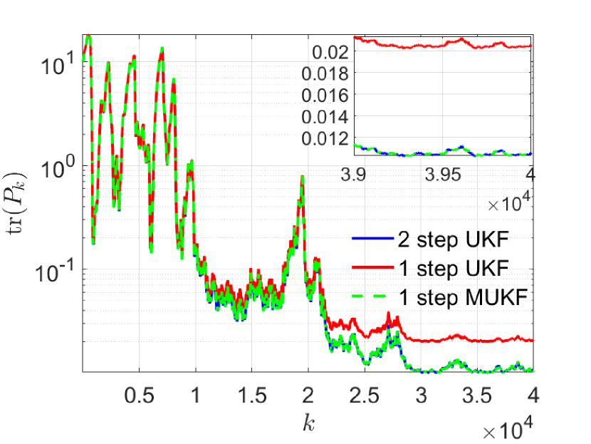
Figure 1: Example VI.1. Trace of the posterior covariance computed using the two-step UKF, the one-step UKF, and the one-step MUKF on a log scale with a zoomed-in inset showing the last 1000 steps of the simulation. Note that the one-step MUKF recovers the accuracy of the two-step UKF.

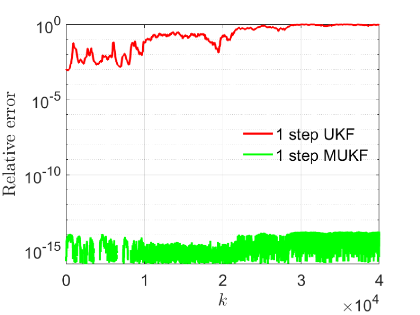
Figure 2: Example VI.1. Relative error in the trace of the posterior covariance computed using the one-step UKF, and the one-step MUKF with respect to the two-step UKF. Note that the posterior covariance computed by the one-step MUKF is numerically within the machine precision of the two-step UKF posterior covariance, whereas the posterior covariance computed by the one-step UKF is almost twice the two-step UKF posterior covariance.

Example VI.2

Lorenz System. Consider the Lorenz system

$$\begin{bmatrix}\dot{x}_{1}\\ \dot{x}_{2}\\ \dot{x}_{3}\end{bmatrix}=\begin{bmatrix}\sigma(x_{2}-x_{1})\\ x_{1}(\rho-x_{3})-x_{2}\\ x_{1}x_{2}-\beta x_{3}\end{bmatrix},$$ (48)

which exhibits a choatic behaviour for $\sigma=10,$ $\rho=28,$ and $\beta=8/3$. The Lorenz system (48) is integrated using the forward Euler method with step size $T_{\rm s}=0.01.$ Let the discrete system be modeled as

$$x_{k+1}=f(x_{k})+w_{k},$$ (49)

where

$$f(x)\stackrel{{\scriptstyle\triangle}}{{=}}x+T_{\rm s}\begin{bmatrix}\sigma(x_{2}-x_{1})\\ x_{1}(\rho-x_{3})-x_{2}\\ x_{1}x_{2}-\beta x_{3}\end{bmatrix}$$ (50)

and $w_{k}\sim{\mathcal{N}}(0,Q_{k}).$ For all $k\geq 0$, let

$$y_{k}=Cx_{k}+v_{k},$$ (51)

where $C\stackrel{{\scriptstyle\triangle}}{{=}}[0\ 1\ 0]$ and $v_{k}\sim{\mathcal{N}}(0,R_{k}).$ For all $k\geq 0,$ let $Q_{k}=0.01I_{2}$ and $R_{k}=10^{-4}.$ Furthermore, let $x(0)=[1\ 1\ 1]^{\rm T}$ and $P_{0|0}=I_{3}$.

Letting $\alpha=1.5$ in the two-step UKF, the one-step UKF, and the one-step MUKF, Figure 3 shows the trace of the posterior covariance computed by the three filters. Note that one-step UKF posterior covariance is larger than the two-step UKF posterior covariance, whereas the one-step UKF recovers the two-step posterior covariance in spite of generating only one ensemble per step. Figure 4 shows the relative error of the one-step UKF and the one-step MUKF posterior covariance relative to the two-step UKF. Note that, in this particular example, the one-step UKF relative error is almost $15\%$, whereas the one-step MUKF relative error is less than the machine precision, that is, the one-step MUKF recovers the two-step UKF.

This example shows that the one-step MUKF posterior covariance estimate is more accurate than the one-step UKF posterior covariance and is numerically equal to the two-step UKF posterior covariance. $\diamond$

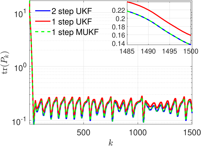
Figure 3: Example VI.2. Trace of the posterior covariance computed using the two-step UKF, the one-step UKF, and the one-step MUKF on a log scale with a zoomed-in inset showing the last 15 steps of the simulation. Note that the one-step MUKF recovers the accuracy of the two-step UKF.

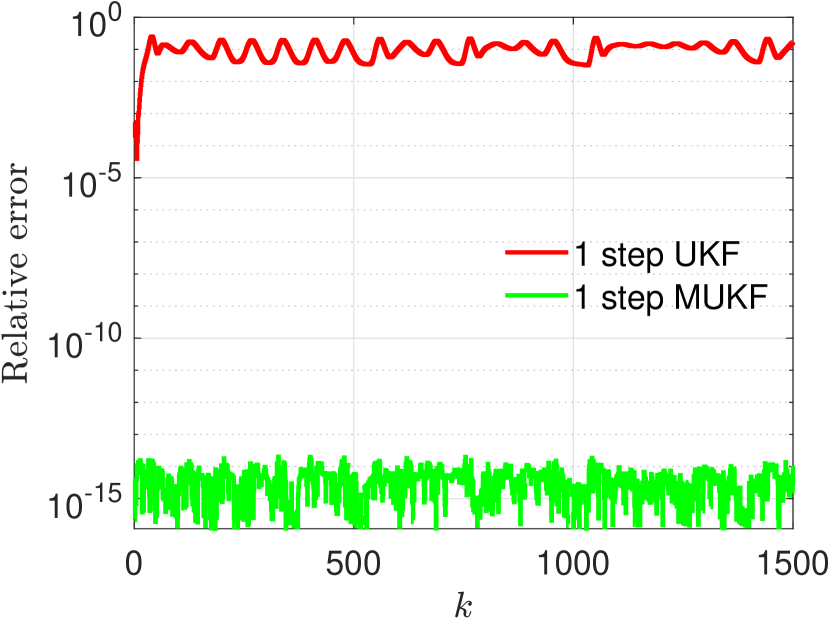
Figure 4: Example VI.2. Relative error in the trace of the posterior covariance computed using the one-step UKF, and the one-step MUKF with respect to the two-step UKF. Note that the posterior covariance computed by the one-step MUKF is numerically within the machine precision of the two-step UKF posterior covariance, whereas the posterior covariance computed by the one-step UKF is about 15 % larger than the two-step UKF posterior covariance.

VII Conclusions

This paper explicitly showed that the two-step UKF specialize to the classical Kalman filter for linear systems, whereas the one-step UKF does not. Consequently, the accuracy of the one-step UKF is inferior than the two-step UKF since the Kalman filter provides the optimal accuracy. Next, a modification of the one-step UKF is presented that recovers the accuracy of the two-step UKF filter in the case of linear systems, that is, it specializes to the classical Kalman filter for linear systems without requiring the second ensemble generation. Finally, it is numerically shown that in nonlinear systems with linear output, the modified one-step UKF recovers the accuracy of the two-step UKF filter.

VIII APPENDIX

VIII-A Proof of Proposition III.1

Proof:

Note that , for $i=1,\ldots,2l_{x}+1,$

$$\hat{x}_{\sigma_{i},k+1} =A_{k}\hat{x}_{\sigma_{i},k}+B_{k}u_{k},$$

$$\hat{y}_{\sigma_{i},k+1} =C_{k+1}\hat{x}_{\sigma_{i},k+1},$$

and thus

$$X_{k+1|k} =A_{k}X_{k|k}+H(B_{k}u_{k}),$$

which implies

$$\hat{x}_{k+1|k}^{\rm UKF}=X_{k+1|k}W=A_{k}\hat{x}+B_{k}u_{k}=\hat{x}_{k+1|k}^{\rm KF}.$$ (52)

The perturbed ensemble is thus

$$\tilde{X}_{k+1|k} =X_{k+1|k}-H(\tilde{X}_{k+1|k}W)$$

$$=A_{k}\begin{bmatrix}0&\alpha\sqrt{l_{x}P}&-\alpha\sqrt{l_{x}P}\end{bmatrix},$$

and thus the prior covariance is

$$P_{k+1|k}^{\rm UKF} =A_{k}\begin{bmatrix}0&\alpha\sqrt{l_{x}P}&-\alpha\sqrt{l_{x}P}\end{bmatrix}W_{\rm d}$$

$$\quad\cdot\begin{bmatrix}0&\alpha\sqrt{l_{x}P}&-\alpha\sqrt{l_{x}P}\end{bmatrix}^{\rm T}A_{k}^{\rm T}+Q_{k}$$

$$=A_{k}PA_{k}^{\rm T}+Q_{k}$$

$$=P_{k+1|k}^{\rm KF}.$$ (53)

The second ensemble is

$$X_{k+1|k}^{\prime}=\Bigg{[}\hat{x}_{k+1|k}^{\rm KF}\quad \hat{x}_{k+1|k}^{\rm KF}+\alpha\sqrt{l_{x}P_{k+1|k}^{\rm KF}}$$

$$\quad\quad\quad\hat{x}_{k+1|k}^{\rm KF}-\alpha\sqrt{l_{x}P_{k+1|k}^{\rm KF}}\Bigg{]},$$

and thus

$$\tilde{X}_{k+1|k}^{\prime} =\begin{bmatrix}0&\alpha\sqrt{l_{x}P_{k+1|k}^{\rm KF}}&-\alpha\sqrt{l_{x}P_{k+1|k}^{\rm KF}}\end{bmatrix},$$

$$\tilde{Y}_{k+1} =C_{k+1}\tilde{X}_{k+1|k}^{\prime}$$

Using (22), (23), it follows that

$$P_{z_{k+1|k+1}}^{\rm UKF} =C_{k+1}\tilde{X}_{k+1|k}^{\prime}W_{\rm d}\tilde{X}_{k+1|k}^{{}^{\prime}\ {\rm T}}C_{k+1}^{\rm T}+R_{k+1}$$

$$=C_{k+1}P_{k+1|k}^{\rm KF}C_{k+1}^{\rm T}+R_{k+1}$$

$$=P_{z_{k+1|k+1}}^{\rm KF},$$ (54)

$$P_{e,z_{k+1|k}}^{\rm UKF} =\tilde{X}_{k+1|k}^{\prime}W_{\rm d}\tilde{Y}_{k+1}^{\rm T}$$

$$=\tilde{X}_{k+1|k}^{\prime}W_{\rm d}\tilde{X}_{k+1|k}^{{}^{\prime}\ {\rm T}}C_{k+1}^{\rm T}$$

$$=P_{k+1|k}^{\rm KF}C_{k+1}^{\rm T}$$

$$=P_{e,z_{k+1|k}}^{\rm KF}.$$ (55)

Finally, (52)-(55) imply (30)-(32). ∎

VIII-B Proof of Proposition IV.1

Proof:

Note that

$$X_{k+1|k} =A_{k}X_{k|k}+H(B_{k}u_{k}),$$

$$Y_{k+1} =C_{k+1}X_{k+1|k}.$$

and thus

$$X_{k+1|k}W =A_{k}\hat{x}_{k|k}+B_{k}u_{k},$$

$$Y_{k+1}W =C_{k+1}A_{k}\hat{x}_{k|k}+C_{k+1}B_{k}u_{k},$$

which implies

$$\tilde{X}_{k+1|k} =A_{k}X_{k}-H(A_{k}\hat{x}_{k|k})$$

$$=A_{k}\begin{bmatrix}0&\alpha\sqrt{l_{x}P_{k|k}^{\rm UKF}}&-\alpha\sqrt{l_{x}P_{k|k}^{\rm UKF}}\end{bmatrix},$$ (56)

$$\tilde{Y}_{k+1} =Y_{k+1}-H(Y_{k+1}W)$$

$$=C_{k+1}\tilde{X}_{k+1}.$$ (57)

The prior covariance is

$$P_{k+1|k}^{\rm UKF} =A_{k}\begin{bmatrix}0&\alpha\sqrt{l_{x}P_{k|k}}&-\alpha\sqrt{l_{x}P_{k|k}}\end{bmatrix}W_{\rm d}$$

$$\quad\cdot\begin{bmatrix}0&\alpha\sqrt{l_{x}P_{k|k}}&-\alpha\sqrt{l_{x}P_{k|k}}\end{bmatrix}^{\rm T}A_{k}^{\rm T}+Q_{k}$$

$$=A_{k}P_{k|k}A_{k}^{\rm T}+Q_{k}$$

$$=P_{k+1|k}.$$

It follows from (34) and (35) that

$$P_{z_{k+1|k+1}}^{\rm UKF} =C_{k+1}\tilde{X}_{k+1}W_{\rm d}\tilde{X}_{k+1}^{\rm T}C_{k+1}^{\rm T}+R_{k+1}$$

$$=C_{k+1}A_{k}P_{k|k}A_{k}^{\rm T}C_{k+1}^{\rm T}+R_{k+1}$$

$$=C_{k+1}(P_{k+1|k}-Q_{k})C_{k+1}^{\rm T}+R_{k+1}$$

$$=C_{k+1}P_{k+1|k}C_{k+1}^{\rm T}-C_{k+1}Q_{k}C_{k+1}^{\rm T}+R_{k+1}$$

$$=P_{z_{k+1|k+1}}-C_{k+1}Q_{k}C_{k+1}^{\rm T},$$ (58)

and

$$P_{e,z_{k+1|k}}^{\rm UKF} =\tilde{X}_{k+1}W_{\rm d}\tilde{Y}_{k+1}^{\rm T}$$

$$=\tilde{X}_{k+1}W_{\rm d}\tilde{X}_{k+1}^{\rm T}C_{k+1}^{\rm T}$$

$$=A_{k}P_{k|k}A_{k}^{\rm T}C_{k+1}^{\rm T}$$

$$=P_{k+1|k}C_{k+1}^{\rm T}-Q_{k}C_{k+1}^{\rm T}$$

$$=P_{e,z_{k+1|k}}-Q_{k}C_{k+1}^{\rm T}.$$ (59)

Since $Q_{k}\neq 0$ and $C_{k}\notin{\mathcal{N}}(Q_{k}),$ it follows that $P_{z_{k+1|k+1}}^{\rm UKF}\neq P_{z_{k+1|k+1}}$ and $P_{e,z_{k+1|k}}^{\rm UKF}\neq P_{e,z_{k+1|k}}$ are missing $C_{k+1}Q_{k}C_{k+1}^{\rm T}$ and $Q_{k}C_{k+1}^{\rm T}$, respectively, , thus implying (40).

To prove (39), note that

$$K_{k+1}^{\rm UKF} =(P_{e,z_{k+1|k}}-Q_{k}C_{k+1}^{\rm T})$$

$$\quad\cdot(P_{z_{k+1|k+1}}-C_{k+1}Q_{k}C_{k+1}^{\rm T})^{-1},$$

$$\neq K_{k+1}.$$ (60)

Finally, since $K_{k+1}$ minimizes ${\rm tr}\,P_{k+1|k+1}$, (60) implies (41). ∎

References

- [1] Dan Simon “Optimal State Estimation: Kalman, H-infinity, and Nonlinear Approaches” John Wiley & Sons, 2006
- [2] Eric A. Wan and Rudolph Van Der Merwe “The Unscented Kalman Filter for Nonlinear Estimation” In Adaptive Systems for Signal Processing, Communications, and Control Symposium, 2000, pp. 153–158 DOI: 10.1109/ASSPCC.2000.882463
- [3] R. Van der Merwe and E A. Wan “The Square-Root Unscented Kalman Filter for State and Parameter-Estimation” In Proceedings of IEEE International Conference on Acoustics, Speech, and Signal Processing 6, 2001, pp. 3461–3464 IEEE DOI: 10.1109/ICASSP.2001.940586
- [4] Edgar Kraft “A quaternion-based unscented Kalman filter for orientation tracking” In Proceedings of the Sixth International Conference of Information Fusion 1.1, 2003, pp. 47–54 IEEE Cairns, Queensland, Australia
- [5] Bingbing Gao, Gaoge Hu, Shesheng Gao, Yongmin Zhong and Chengfan Gu “Multi-sensor optimal data fusion for INS/GNSS/CNS integration based on unscented Kalman filter” In International Journal of Control, Automation and Systems 16.1 Springer, 2018, pp. 129–140
- [6] Hongwen He, Rui Xiong and Jiankun Peng “Real-time estimation of battery state-of-charge with unscented Kalman filter and RTOS mu-COS-II platform” In Applied energy 162 Elsevier, 2016, pp. 1410–1418
- [7] JH Gove and DY Hollinger “Application of a dual unscented Kalman filter for simultaneous state and parameter estimation in problems of surface-atmosphere exchange” In Journal of Geophysical Research: Atmospheres 111.D8 Wiley Online Library, 2006
- [8] Jeffrey L Anderson “An ensemble adjustment Kalman filter for data assimilation” In Monthly weather review 129.12 American Meteorological Society, 2001, pp. 2884–2903
- [9] Simon J Julier and Jeffrey K Uhlmann “New extension of the Kalman filter to nonlinear systems” In Signal processing, sensor fusion, and target recognition VI 3068, 1997, pp. 182–193 International Society for OpticsPhotonics
- [10] Mathieu St-Pierre and Denis Gingras “Comparison between the unscented Kalman filter and the extended Kalman filter for the position estimation module of an integrated navigation information system” In IEEE Intelligent Vehicles Symposium, 2004, 2004, pp. 831–835 IEEE
- [11] Simo Särkkä “Bayesian filtering and smoothing” Cambridge university press, 2013
- [12] Charles F Van Loan “The Ubiquitous Kronecker Product” In Journal of Computational and Applied Mathematics 123.1-2 Elsevier, 2000, pp. 85–100 DOI: 10.1016/S0377-0427(00)00393-9