Supernova search with active learning in ZTF DR3

Abstract

Context. We provide the first results from the complete SNAD adaptive learning pipeline in the context of a broad scope of data from large-scale astronomical surveys.

Aims. The main goal of this work is to explore the potential of adaptive learning techniques in application to big data sets.

Methods. Our SNAD team used Active Anomaly Discovery (AAD) as a tool to search for new supernova (SN) candidates in the photometric data from the first 9.4 months of the Zwicky Transient Facility (ZTF) survey, namely, between March 17 and December 31 2018 (58194 $\leq$ MJD $\leq$ 58483). We analysed 70 ZTF fields at a high galactic latitude and visually inspected 2100 outliers.

Results. This resulted in 104 SN-like objects being found, 57 of which were reported to the Transient Name Server for the first time and with 47 having previously been mentioned in other catalogues, either as SNe with known types or as SN candidates. We visually inspected the multi-colour light curves of the non-catalogued transients and performed fittings with different supernova models to assign it to a probable photometric class: Ia, Ib/c, IIP, IIL, or IIn. Moreover, we also identified unreported slow-evolving transients that are good superluminous SN candidates, along with a few other non-catalogued objects, such as red dwarf flares and active galactic nuclei.

Conclusions. Beyond confirming the effectiveness of human-machine integration underlying the AAD strategy, our results shed light on potential leaks in currently available pipelines. These findings can help avoid similar losses in future large-scale astronomical surveys. Furthermore, the algorithm enables direct searches of any type of data and based on any definition of an anomaly set by the expert.

1 Introduction

The advent of modern astronomical surveys, initiated by the Sloan Digital Sky Survey (SDSS, Blanton et al., 2017) and further propelled by the Zwicky Transient Facility (ZTF, Bellm et al., 2019), has popularised the use of automated machine learning methods (Baron, 2019). This shift towards a data-driven approach to astronomical research has been developing swiftly for supervised learning tasks in the areas of classification (see e.g. Carleo et al., 2019; Ishida, 2019; Malik et al., 2022, and references therein) and regression (e.g. Krone-Martins et al., 2014; Pasquet et al., 2019; Cabayol et al., 2021; Henghes et al., 2021; Chen et al., 2022).

Nevertheless, thanks to the availability of continuous scans of the sky with instruments that are capable of achieving unprecedented resolution, it is natural to expect that new and interesting astrophysical sources will continue to be detected. The challenge then becomes developing automated unsupervised learning strategies that can successfully identify such sources among large and complex data sets. The astronomical community has devoted significant efforts to this direction. For example, Pruzhinskaya et al. (2019) applied the isolation forest (IF, Liu et al., 2008) algorithm to identify contaminants in the Open Supernova Catalog (Guillochon et al., 2017). Malanchev et al. (2021b) used four different anomaly detection (AD) algorithms and a comprehensive feature extraction process to identify unusual light curves in the third ZTF data release (DR). In searching for changing-state active galactic nuclei (AGNs), Sánchez-Sáez et al. (2021) identified 75 promising candidates by combining dimensionality reduction via deep learning with IF. Storey-Fisher et al. (2021) applied a Wasserstein generative adversarial network on nearly one million optical galaxy images in the Hyper Suprime-Cam survey. Martínez-Galarza et al. (2021) combined tree-based AD and manifold learning to identify sets of unusual light curves in Kepler data. Chan et al. (2022) applied a similar strategy to identify anomalous periodic variables in ZTF data. Sarkar et al. (2022) used the Earth as an anomaly example in order to estimate the habitability of exoplanets using a multi-stage memetic algorithm. Kovačević et al. (2022) used self-organising maps to analyse temporal-only parameters computed from $\gtrapprox 10^{5}$ sources from the Exploring the X-ray Transient and variable Sky catalogue and Aleo et al. (2022b) used simulated light curves to search for counterparts in ZTF DR4, identifying 11 non-catalogued transients.

Despite such promising results, all AD studies need to deal with the discrepancy between the statistical definition of an outlier (which directly affects the output from traditional machine learning models) and astrophysically interesting anomalies (unforeseen or yet to be confirmed events generated by unusual astrophysical phenomena). In large data sets, outliers tend to dominate the set of objects with high anomaly scores (Malanchev et al., 2021b). Adaptive learning techniques are aimed at sequentially incorporating expert knowledge in machine learning models (see e.g. Ishida et al., 2021; Lochner & Bassett, 2021). The SNAD team has been consistently improving and testing such an adaptive learning strategy, whereby at each iteration, a binary reply from the expert is incorporated into the weight calculation of an IF model, producing updated anomaly scores. The active anomaly discovery (AAD, Das et al., 2017) algorithm has proven to be effective in its first application to real data (Ishida et al., 2021). In this work, we stress test the effectiveness of this strategy by applying it to light curves from ZTF DR3. Considering as anomalies any light curves that resemble those of supernovae (SNe), our experts scanned 70 ZTF fields searching for uncatalogued or anomalous transients.

This paper is organised as follows. Section 2 describes the data selection process (2.1), learning algorithm (2.2), and a summary of the results (2.3). In Section 3, we present the results of our light-curve modelling for a subset of the newly reported transients. Section 4 presents an in-depth discussion on superluminous supernova (SLSN) candidates (4.1), along with a complete set of labels within the SNAD viewer knowledge database (4.2) and a description of other non-catalogued objects found during our search (4.3). We present our conclusions in Section 5. Additionally, the complete SNAD catalogue of discovered transients is shown in Appendix A. Appendix B shows light curves and corresponding fit models for SNAD objects. Appendix C gives a glimpse of the domain knowledge database within the SNAD viewer.

2 Supernova search

2.1 ZTF data and field selection

We analysed photometric data from the first 9.4 months of the ZTF survey, between 2018 March 17 and December 31 (58194 $\leq$ MJD $\leq$ 58483). This period includes data from the ZTF private survey, thus offering a better cadence than the rest of DR3. However, the expert analysis of discovered SNe (see Section 3) used more complete light curves from ZTF DR8.

Given the higher probability of finding SNe in low extinction regions, we analysed only those fields with centres at $>20^{\circ}$ above the galactic plane. The distribution of the 70 fields considered in this work is given in Fig. 1.

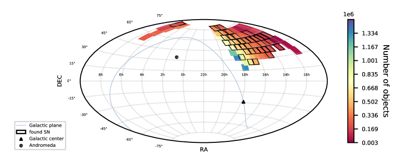
Figure 1: Sky map in equatorial coordinates with plotted positions of ZTF fields analysed in this work, the colour bar shows the number of objects in each field. Fields with detected supernova candidates are highlighted with bold black boundaries. The blue curve denotes the galactic plane. The black triangle marks the galactic centre and the black circle corresponds to the position of the Andromeda galaxy.

Each one of the selected fields contains from a few thousand to a little more than a million objects with at least 100 photometric points in $zr$-band (catflags $=0$), thus comprising $\sim$26.5 million light curves in total. Each object is characterised by ZTF Object ID (OID). This identifier is unique only within each field and each band, therefore the same source observed in different fields and in different bands can have several OIDs.

Per each OID, we extracted 42 $zr$-band light curve features including magnitude amplitude, Stetson $K$ coefficient (Stetson, 1996), standard deviation of Lomb–Scargle periodogram (Lomb, 1976; Scargle, 1982), and others. A full description of all features used is given in Malanchev et al. (2021b) and Malanchev (2021a).

2.2 Active anomaly discovery

Recommendation systems are automatic algorithms whose goal is to minimise the cost of labelling tasks and, at the same time, to optimise classification or anomaly detection results. In this work, we use the AAD algorithm proposed by Das et al. (2017). It starts with a traditional IF and sequentially presents the object with highest anomaly score to the expert. If the expert judges a particular outlier not to be interesting, the weights of each decision path is changed to accommodate this new information and the data is passed through the slightly modified forest. The process is repeated until a certain budget has been reached. This framework was first applied to a simulated as well as a small real data set by Ishida et al. (2021).

Here, we present the first application of AAD to a significantly larger data set of real observations ($\sim$26.5 million light curves). Since the algorithm can adapt to the expert’s opinion, it can be used for a targeted search of transients of a certain type (e.g. SNe). Therefore, in this analysis, a human expert considered only SN-like candidates as anomalies; all other objects proposed by the algorithm are rejected by the expert as ’uninteresting’ (i.e. ‘yes’ and ‘no’ in the AAD interface). For each field, the expert has gone through a total budget of 30 objects.

In order to enable a smooth interaction between our experts and the AAD algorithm when dealing with such a large data set, we developed the SNAD knowledge database (Malanchev et al., 2022), a framework used by our experts to log their input as one entry in a tailored set of labels (see further details in Section 4.2). For each one of the ZTF fields, our experts went through 30 objects registering their feedback as a binary answer. The distribution of objects by type for each of the 35 fields containing SNe or SN candidate is given in Fig. 2. Each line represents one AAD run with 30 queries in the order of appearance to the expert. The colour denotes the assigned tag, namely, whether it is a supernova, artefact, or other type of object.

Figure 2: Distribution of objects by type for each of the 35 fields containing supernova or supernova candidate. Each line represents one AAD run with 30 queries. Red, green, and beige colours denote the supernova candidate, artefact or other type of object, respectively. Fields are ordered by the number of objects in them, from 135681 (bottom line) to 856453 (top line).

In what follows, we further investigate the most interesting objects we encountered. The source code is publicly available as a part of zwad (Malanchev et al., 2021a) GitHub repository.

2.3 Results

We visually inspected 2100 ($70\times 30$) outliers. Among them, we found 104 SN-like objects, 57 of which were reported for the first time and 47 were previously mentioned in other catalogues, either as SNe of known types or as SN candidates (see Section 4.2 for other type of objects found). Sources which were not previously mentioned in the Transient Name Server (TNS) received an internal SNAD name, were added to the SNAD catalogue, and reported to TNS. The full list of transients found by the AAD algorithm is given in Table LABEL:tab:sn_list. Column 1 contains the internal SNAD names of the non-catalogued SN-like candidates. The equatorial coordinates are given in columns 2 and 3. In column 4, we list the ZTF OIDs. The suggested transient type is defined in column 5. If the object also exists in ZTF alerts, the corresponding target alert name is given in column 6. Column 7 contains the TNS name. Column 8 reports OIDs output by the pipeline that corresponds to the same astrophysical source.

Figure 1 shows the distribution of inspected fields on the sky in equatorial coordinates, along with the corresponding number of objects. There are 35 fields with detected SN candidates that are outlined in black. Naively, we would expect that fields with supernovae should be concentrated at the regions further away from the galactic plane and galactic centre. However, we observe that they are located in the middle galactic longitude and latitude. This can be explained by the smaller number of observations in more extragalactic regions. Moreover, the number of objects in different fields varies from a few thousand to more than a million, and the fact that we did not detect any SN in regions with more than a million objects (only three regions), which are also very close to the Milky Way centre, may indicate that the budget of 30 objects was not enough for the AAD to adapt and ideally should be scaled according to the number of objects in the field.

Among the previously reported supernovae candidates, there are 14 SNe Ia, 13 possible SNe, 7 SNe II, 3 SNe Ic, 2 SNe IIP, and 1 SN Ib; the remaining 7 catalogued SNe belong to the rare supernova classes considered as anomalies in Pruzhinskaya et al. (2019); Ishida et al. (2021), namely, 2 SNe IIb, 1 SN Ia Pec, 1 SN Ia-91bg, 1 SN Ic BL, 1 SN IIn, and 1 SLSN-I. To compare the efficiency of the AAD algorithm in searching for more rare and therefore potentially interesting objects, we recorded the number of spectroscopically confirmed SNe found in this work and discovered by different groups, in the ZTF data, according to TNS for the same period of time (58194 $\leq$ MJD $\leq$ 58483), as shown in Table 1. The fraction of rare SN types among the total number is $\sim$21% for AAD discoveries and $\sim$10%  for general TNS findings.

Table 1: Sub-populations of spectroscopically confirmed supernovae, found in this work (AAD) and total reported in TNS (TNS) for the same time period. TNS numbers report findings within ZTF data only.

Type	AAD (%)	TNS (%)
SN Ia	14 (41)	591 (69)
SN II	7 (20)	124 (14)
SN IIP	2 (6)	25 (3)
SN Ib	1 (3)	16 (2)
SN Ic	3 (9)	20 (2)
Rare SN types
SN Ia Pec	1 (3)	11 (1)
SN Ia-91bg	1 (3)	7 (1)
SN IIb	2 (6)	13 (2)
SN Ic BL	1 (3)	12 (1)
SN IIn	1 (3)	25 (3)
SLSN-I	1 (3)	15 (2)
Total:	34 (100)	859 (100)

Non-catalogued SN-like objects are listed in the beginning of Table LABEL:tab:sn_list. We note that 15 SNAD possible supernovae (PSNe) are missing in the official ZTF alert stream (Table LABEL:tab:sn_list, column 6). Missed transients have peak $zr$ magnitude $\sim$19.5–20 mag, which is indeed quite low, but still compatible with those of some other SNAD transients detected by the alert system. Furthermore, some of our candidates (e.g. SNAD128, SNAD165) have well-sampled early light curves which is of interest for surveys such as the Young Supernova Experiment (Jones et al., 2021).

3 Supernova modelling

We used the Python library sncosmo to obtain a preliminary photometric classification for SNAD objects. Their light curves were fitted with Peter Nugent’s supernova models, which cover the main SN types (Ia, Ib/c, IIP, IIL, IIn). Nugent’s models are simple spectral time series that can be scaled up and down. The model parameters are the redshift, $z$, the observer-frame time corresponding to the source’s zero phase, $t_{0}$, and the amplitude. The zero phase is defined relative to the explosion moment and the observed time, $t,$ is related to phase via $t=t_{0}+{\rm phase}\times(1+z)$.

In order to perform a preliminary fit, we used only the $zr$-band from DR8. We subtracted the reference magnitude from ZTF light curves, thus roughly accounting for the host galaxy contamination. The reference magnitude was retrieved from ZTF archival data and listed in the SNAD catalogue. We also corrected for a line-of-sight reddening in the Milky Way galaxy using Schlafly & Finkbeiner (2011) estimates. For sources holding SDSS DR16 (Ahumada et al., 2020) photometric redshift of a host galaxy at the source position, we fixed the redshift to this value. If this was not available, we adopted $[-15;-22]$ as an acceptable range for the supernova absolute magnitude (Richardson et al., 2014) and then, using the maximum apparent magnitude, roughly transformed it to the corresponding redshift range. We applied a $\chi^{2}$ criterion to choose the best-fit model for each SNAD object. Results of the light curve fit are given in Appendix B, the best-fit model for each SNAD transient is listed in column 5 of Table LABEL:tab:sn_list.

It should be noted that we did not intend to make a detailed fit, but, rather, to show that the candidate light curves, selected initially by eye, can be satisfactorily fitted by different supernova models. That is why only one band ($zr$) has been used in the fit. Also, we did not take into account the possible extinction in host galaxies of the candidates, therefore, our fit is less accurate for highly reddened objects. Moreover, the redshift we assigned to some host galaxies is photometric, which is another source of uncertainty. Finally, the model itself is rather simple and limited in wavelength and time range. As a result of these conscious simplifications and assumptions, the obtained absolute magnitude for some of the objects is not typical for normal SNe (e.g. SNAD122, $M_{r}\rm{(IIP)}\simeq-22.6$ mag) and we cannot trust the classification in those cases. However, this simple fit is enough to show that a few transients have anomalously wide light curves when compared to normal SNe, making them candidates to the SLSN class (Section 4.1).

Although this classification should be treated with caution, it follows closely the behaviour of light curves with a sufficient number of observations before and after maximum light. Using the sncosmo library, we also performed a multi-band light-curve fit for a few objects with the models suggested by the preliminary classification. The parameters of the fit are $z$, $t_{0}$, and the amplitude. Then, SNAD112, SNAD142, SNAD165, and SNAD137 fitted by Nugent’s Type Ia, IIP, Ibc, and IIn models are given in Fig. 3, 4, 5, and 6, respectively. The quality of the fit allows us to conclude that those supernovae belong to the suggested types.

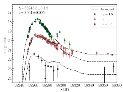
Figure 3: Light curve fit of SNAD112 by Nugent’s Type Ia supernova model. Observational data correspond to OIDs: 796101400003999 ($zg$), 796201400007564 ($zr$), 796301400021875 ($zi$), and 797304300009092 ($zi$).

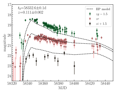
Figure 4: Light curve fit of SNAD142 by Nugent’s Type IIP supernova model. Observational data correspond to OIDs: 826102200028756 ($zg$), 826202200030732 ($zr$), and 826302200021568 ($zi$).

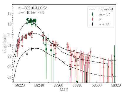
Figure 5: Light curve fit of SNAD165 by Nugent’s Type Ibc supernova model. Observational data correspond to OIDs: 763104300002058 ($zg$), 763204300004087 ($zr$), and 763304300014301 ($zi$).

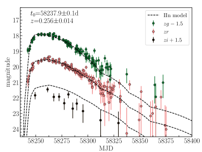
Figure 6: Light curve fit of SNAD137 by Nugent’s Type IIn supernova model. Observational data correspond to OIDs: 825102200009050 ($zg$), 825202200039582 ($zr$), and 825302200018371 ($zi$).

4 Discussion

4.1 Superluminous supernovae candidates

Four supernova candidates from our list possess significantly broader light curves in comparison with Nugent’s models and other candidates: SNAD120, SNAD121, SNAD160, and SNAD187 (see Appendix B). In this section we explore the possibility of these objects belonging to the SLSN class.

SNAD120 (AT2018lxa) is located at $\alpha\leavevmode\nobreak\ =\leavevmode\nobreak\ 17^{h}00^{m}16.296^{s}$, $\delta=+70^{\circ}30^{{}^{\prime}}49.55^{{}^{\prime\prime}}$. In the official ZTF alert stream, it is denoted as ZTF18aazydub. According to  Strotjohann et al. (2021), the transient has a spectroscopic redshift of $z_{\rm sp}=0.202$ and was classified as SN IIn. Assuming this redshift, the estimated absolute magnitude at maximum brightness is $M_{r}\simeq-20.5$ mag, which is slightly dimmer than the threshold of $-21$ mag established for SLSNe (Gal-Yam, 2012).

SNAD121 (AT2018lxb, ZTF18abklshn) is located at $\alpha\leavevmode\nobreak\ =\leavevmode\nobreak\ 16^{h}33^{m}19.937^{s}$, $\delta=+71^{\circ}06^{{}^{\prime}}54.50^{{}^{\prime\prime}}$. On archival images provided by the Legacy Surveys Sky Viewer, a possible host is detected with an estimated photometric redshift of $z_{\rm ph}=0.240\pm 0.166$ (Zhou et al., 2021). Taking into account redshift uncertainty, the absolute magnitude of this source is estimated to be brighter than $-21$ mag, thus, it is compatible with SLSNe.

SNAD160 (AT2018lzi, ZTF18aautopz) is located at $\alpha\leavevmode\nobreak\ =\leavevmode\nobreak\ 13^{h}43^{m}53.357^{s}$, $\delta=+61^{\circ}33^{{}^{\prime}}17.24^{{}^{\prime\prime}}$. The ALeRCE ZTF Explorer automatically classified ZTF18aautopz as a SLSN. The spectroscopic redshift is $z_{\rm sp}=0.295$ (Strotjohann et al., 2021), which gives $M_{r}\simeq-21.6$ mag at maximum light. SNAD160 is reported by SNAD team in Pruzhinskaya et al. (2022) as a possible pair-instability supernova – a theoretical class of thermonuclear explosions which takes place at the end of life of very massive stars with highly increased production of ⁵⁶Ni (e.g. Gal-Yam, 2019; Kozyreva et al., 2014).

SNAD187 (AT2018mcb, ZTF18aaqctvg) is located at $\alpha\leavevmode\nobreak\ =\leavevmode\nobreak\ 13^{h}53^{m}7.366^{s}$, $\delta=+40^{\circ}48^{{}^{\prime}}7.42^{{}^{\prime\prime}}$. There are several photometric redshift estimations of its possible host provided by different surveys: $z_{\rm ph}=0.204\pm 0.084$ by the Legacy Surveys Sky Viewer (Zhou et al., 2021), $z_{\rm ph}=0.343\pm 0.128$ by SDSS DR16 (Ahumada et al., 2020), and $z_{\rm ph}\simeq 0.201$ by Gaia DR3 (Gaia Collaboration, 2022). Also, according to Gaia variability classification results there is an AGN at the transient position (Gaia Collaboration, 2022). It is possible that SNAD187 is not associated with the host AGN activity and could be a SLSN. Recently, the ANTARES broker AD filter reported the discovery of a SLSN — SN 2022mnj at the central region of an AGN (Aleo et al. 2022a; Ashall 2022; see also Moriya et al. 2017).

Figure 7 shows the observed light curves of SNAD120, SNAD121, SNAD160, and SNAD187 in the $zr$-band in comparison with SN 2006gy (Smith et al., 2007) — one of the brightest among the well-studied SLSNe, shifted to $z=0.3$ and 0.4. SN 2006gy has a very broad light curve, but it is clear that the SNAD candidates have even broader light curves, making them really peculiar objects among known SNe. The discovery of four slow-evolving transients among the SNAD objects, non-reported by previous searches provides clear evidence that the AAD is efficient in searching for rare classes of astronomical objects within large and complex data sets.

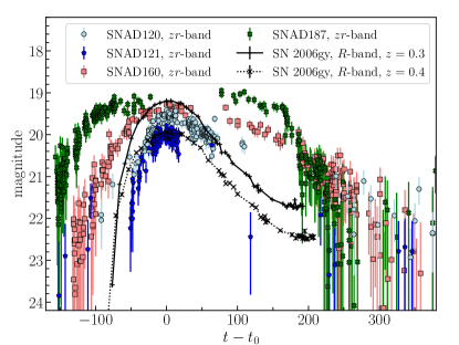
Figure 7: Light curves of SNAD SLSN candidates in $zr$-band in comparison with the R-band light curve of well-studied SLSN SN 2006gy shifted to $z=0.3$ (black pluses) and $z=0.4$ (black crosses). The observed magnitudes of SN 2006gy are taken from Smith et al. (2007). All the light curves are shown relative to the maximum light.

4.2 SNAD knowledge database

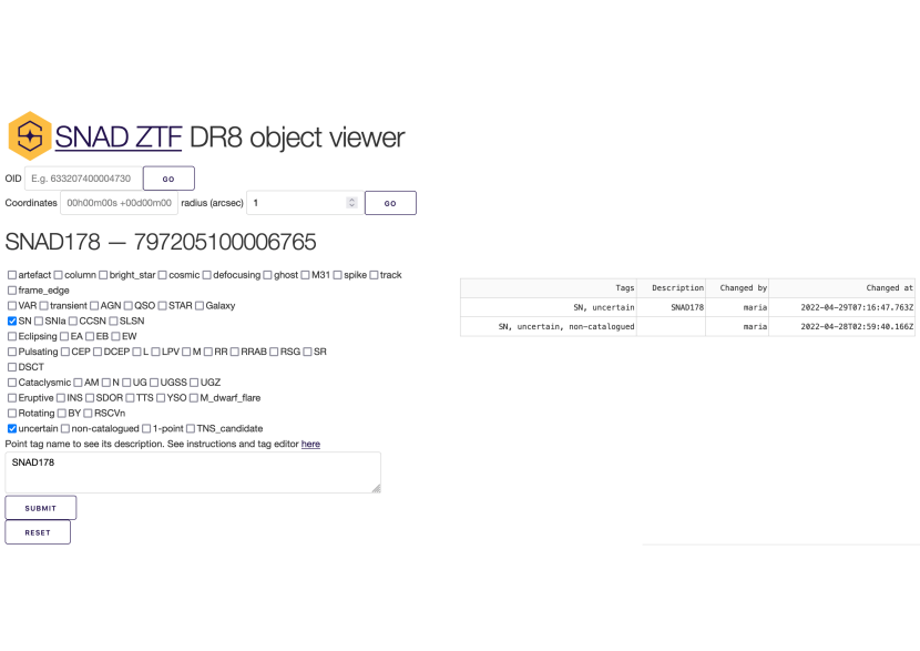
Figure 23: SNAD ZTF viewer tags and logs on the example of SNAD178.

Beyond the transient candidates discussed previously, this work also produced a valuable knowledge database incorporated within the SNAD viewer (Malanchev et al., 2022). The viewer is a specially designed web-interface, which allows the expert to visualise ZTF DR light curves, provides access to the individual exposure images, and performs cross-matches with different databases and catalogues. For authorised users, there is a possibility to assign the labels (tags) to ZTF objects (see Fig. 23).

We defined a system of tags that includes some general classes: variable star of unspecified type (VAR), transient (transient), active galactic nucleus (AGN), quasar (QSO), normal star without strong variability (STAR), and galaxy (Galaxy), as well as the most popular types and subtypes of variable stars and transients, such as:

• Supernova (SN): Type Ia supernova (SNIa), core-collapse supernova (CCSN), and super-luminous supernova (SLSN);

• Eclipsing variable (Eclipsing): $\beta$ Persei-type (Algol) eclipsing system (EA), $\beta$ Lyrae-type eclipsing system (EB), and W Ursae Majoris-type eclipsing variable (EW);

• Pulsating variable (Pulsating): cepheid (CEP), classical cepheid or $\delta$ Cephei-type variable (DCEP), slow irregular variable (L), long period variable (LPV), $o$ Ceti-type (Mira) variable (M), variable of the RR Lyrae type (RR), RR Lyrae variable with asymmetric light curve (RRAB), red supergiant (RSG), semi-regular variable (SR), and variable of the $\delta$ Scuti type (DSCT);

• Cataclysmic variable (Cataclysmic): AM Herculis-type variable (AM), nova (N), U Geminorum-type variable or dwarf nova (UG), SS Cygni-type variable (UGSS), and Z Camelopardalis-type star (UGZ);

• Eruptive variable (Eruptive): Orion variable with rapid light variations (INS), variable of the S Doradus type (SDOR), T Tauri star (TTS), young stellar object of unspecified variable type (YSO), M dwarf flare (M_dwarf_flare);

• Rotating variable (Rotating): BY Draconis-type variable (BY), RS Canum Venaticorum-type binary system (RSCVn).

There are a few custom tags for internal purposes, such as transients with one outlier point (1-point) or candidates to be send to TNS (TNS_candidate). Also, tags of non-astrophysical origin such as artefacts and their subtypes are present. Several tags can be assigned to one object, the history of tag changes is also stored in the database (Fig. 23, on the right).

The choice of tags is determined by the experts, based on the most frequent types of objects appearing in the output of the AD algorithms and also determined by the project needs. Therefore, we do not claim to be complete in covering all possible types of variables and transients.

During the supernova search a total of 1482 objects were labelled. Despite the fact that ZTF data processing pipeline includes a procedure to separate the astrophysical events from bogus ones, namely, false positive detections (Masci et al., 2019), fields with SNe consists of $\sim$45%  of artefacts. Examples of found artefacts are given in Fig. 8.

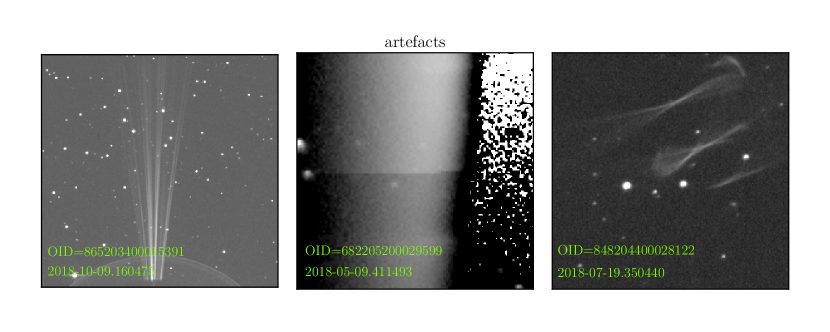
Figure 8: Examples of artefacts found during the supernova search with AAD. The outlier is located in the image centre. The image sizes are 600$\times$600, 100$\times$100, and 200$\times$200 CCD pixels, respectively.

For real variables, among the most common types in fields containing SNe, are eclipsing ($N=51$, $\sim$5%) and pulsating ($N=53$, $\sim$5%) variables, as well as AGNs ($N=176$, $\sim$17%). The assigned labels can be used to further improve the ZTF pre-processing pipeline (in case of artefacts) as well as for machine-learning classification tasks (in case of astrophysical labels).

4.3 Other non-catalogued objects

During the supernova search, a number of interesting non-catalogued objects of other types have been found. Among those there are red dwarf flares, namely, transients caused by the sudden release of stored magnetic energy from surface magnetic loops into the outer stellar atmosphere (Pettersen, 1989; Haisch et al., 1991), and AGNs. For example, a two-peak flare of a red dwarf, OID = 726209400028833, located at a distance of $\sim$162 pc (Bailer-Jones et al., 2018) is shown in Fig. 9. The amplitude of the flare is $\sim$1.8 mag, the minimum duration is $\sim$46 minutes. There are many unsolved questions related to flare physics, red dwarf distribution in the Galaxy, and habitability of host planets, which can benefit from a systematic study of a large sample of such events (e.g. Segura et al. 2010; Engle & Guinan 2011; France et al. 2013; Webb et al. 2021). Moreover, good observational cadence of the flare ($\sim$70 points in 46 min) also opens up a possibility to search for fast transients in ZTF data.

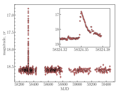
Figure 9: Light curve of a complex red dwarf flare, OID: 726209400028833 ($zr$). Inset plot shows a zoomed high-cadence light curve with two-peaks flare.

Another interesting object, OID = 676213300006792, located at a distance of $\sim$234 pc (Bailer-Jones et al., 2018), shows two outbursts, one of which is observed at a high frequency (see Fig. 10). Based on its SDSS spectrum, 676213300006792 was previously identified as a white dwarf-main sequence binary with a secondary M-dwarf companion (Liu et al., 2012). 676213300006792 is a weak UV source and does not appear in any X-ray database. Its SDSS spectrum does not show a significant $H_{\alpha}$ emission. The high cadence $zg$-band light curve shows a periodicity with $P\simeq 4.25$ minutes, just before the flare. We assume that there is no stable mass transfer in the system, and the M-dwarf has not overflowed its Roche lobe. We attribute the outbursts to the low accretion rate of the unstable stellar wind on the white dwarf during the increase in magnetic activity from the M-dwarf. The periodic variation before the flare may be related to a hot spot in the temporary accretion disc.

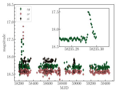
Figure 10: Light curves of a white dwarf-M-dwarf binary system. Observational data correspond to OIDs: 676113300003418 ($zg$), 676213300006792 ($zr$), and 676313300009030 ($zi$). Inset plot shows a zoomed high-cadence $zg$-band light curve with flare and possible periodicity.

Other non-catalogued objects include candidates for AGNs (e.g. Fig. 11) and variable stars of different nature (e.g. eclipsing binary candidate in Fig. 12). All these objects can be studied separately in the future by the domain experts.

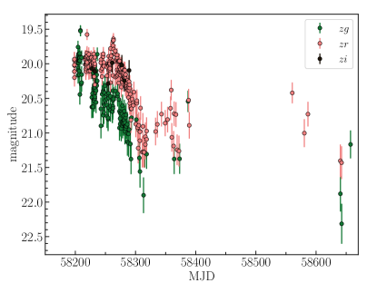
Figure 11: Light curves of an AGN candidate. Observational data correspond to OIDs: 763114100009685 ($zg$), 763214100020120 ($zr$), and 763314100028589 ($zi$).

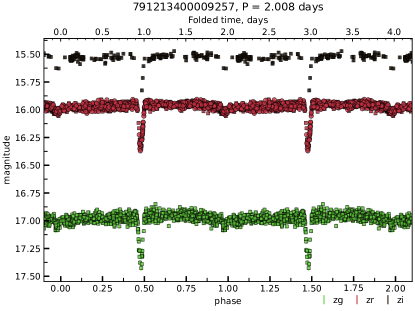
Figure 12: Folded light curves of a non-catalogued eclipsing binary candidate. Observational data correspond to OIDs: 791113400002334, 792116300002277 ($zg$); 791213400009257, 792216300003876 ($zr$); 791313400005610, and 792316300013740 ($zi$).

5 Conclusions

In this work, we provide the first results from the complete SNAD adaptive learning pipeline in the presence of big data from large-scale astronomical surveys. The SNAD team became aware of the existence of non-reported supernova candidates within the ZTF DRs once they appeared in a non-targeted anomaly detection search (Malanchev et al., 2021b). A new experiment was then designed to develop a tailored machine learning model which would explore this possibility by taking advantage of the SNAD adaptive learning pipeline (Ishida et al., 2021) and our experts’ long-term experience studying supernovae.

We selected 70 ZTF fields in high galactic latitude, employed a series of quality cuts followed by designed feature extraction (Section 2.1). The resulting homogeneous feature sets (one per field) were submitted independently of 30 iterations of the active anomaly discovery algorithm, where at each iteration, the domain expert would input a positive feedback to any outlier whose light curve resembles a SN and a negative one otherwise. During this process, human-assigned labels were added to the SNAD knowledge database, opening the way for future deeper analysis of the same data (Section 4.2). From the 2100 objects visually inspected, we found 104 SN-like events, 57 of which were reported for the first time. These transients received an internal name, were reported to TNS and added to the SNAD catalogue (see Section 2.3).

In order to evaluate probable classification types for the newly found transients, we performed light curve fits using different supernova models (Section 3). Among the newly found transients, we reported three objects (SNAD121, SNAD160 and SNAD187) with broad, slowly evolving light curves that stand as promising superluminous supernova candidates (see Fig. 7 and Pruzhinskaya et al., 2022).

Despite the fact that the AAD was aimed at supernova search, other potentially interesting objects have been found, including non-catalogued AGNs and red dwarf flares. The high cadence data of discovered flares opens the possibility of searching for fast transients in ZTF. Moreover, the visual inspection of AAD outliers during the SN search led to the creation of the SNAD knowledge database that can be used for different machine learning tasks in the future.

The overall efficiency of the pipeline is highly dependent on the total number of objects being analysed, feature choices, and maximum iterations budget, among other parameters. Nevertheless, the results presented here confirm the effectiveness of adaptive learning approaches in filtering large astronomical data sets for expert analysis. They reveal important characteristics of ZTF data releases that ought to be further scrutinised to avoid similar losses in the future (Aleo et al., 2022b).

Appendix A AAD results

We report the complete set of SN-like transients shown to the expert by the AAD pipeline below.

Table 2: Complete list of supernovae and supernova candidates found by active anomaly discovery algorithm in ZTF DR3.

№	Name	R.A.	Dec.	OID	Type∗	Target alert name	Other names	Remarks
1	SNAD101	247.45543	24.77282	633207400004730	IIn	ZTF18abqkqdm	AT 2018lwh
2	SNAD102	245.05375	28.38220	633216300024691	IIn	ZTF18abdgwos	AT 2018lwi
3	SNAD103	219.83787	47.40378	758205100001118	IIP		AT 2018lwj
4	SNAD104	218.91620	46.38441	758205400019523	IIP	ZTF18aawqbuc	AT 2018lwk
5	SNAD105	218.34626	49.22553	758209200010983	Ibc		AT 2018lwl
6	SNAD106	219.41935	50.16706	758213400002862	Ia		AT 2018lwm
7	SNAD107	254.41703	44.29804	762202300014913	Ibc		AT 2018lwn
8	SNAD108	257.84004	48.21127	762209400037712	Ia	ZTF18abauopo	AT 2018lwo
9	SNAD109	191.17808	54.31252	790207100016149	IIn		AT 2018lwp
10	SNAD111	263.42634	52.62203	796201100002136	Ibc	ZTF18abdldos	AT 2018lwr
11	SNAD112	263.37725	51.25848	796201400007564	Ia	ZTF18aaubejv	AT 2018lws
12	SNAD113	254.81890	58.37547	796215200010831	Ia	ZTF18abmmdnx	AT 2018lwt	825204400024382
13	SNAD113	254.81983	58.37536	825204400024382	Ia	ZTF18abmmdnx	AT 2018lwt	796215200010831
14	SNAD114	257.27308	57.55380	796215400002705	IIn	ZTF18aawkaod	AT 2018lwu
15	SNAD115	252.82337	62.83286	824209400038197	IIn	ZTF18absufwv	AT 2018lwv
16	SNAD116	242.29542	62.48738	824212400005043	Ia	ZTF18abklrmo	AT 2018lww
17	SNAD117	254.04870	65.01217	824213100016761	IIP	ZTF18aanbiig	AT 2018lwx
18	SNAD119	245.80060	68.69152	847207200014161	IIn	ZTF18abgujpm	AT 2018lwz
19	SNAD120	255.06791	70.51376	847209200012956	IIP	ZTF18aazydub	AT 2018lxa
20	SNAD121	248.33307	71.11514	847211100017171	IIP	ZTF18abklshn	AT 2018lxb
21	SNAD122	217.38363	33.54185	676212400013135	IIP	ZTF18aawqcqz	AT 2018lxg
22	SNAD123	230.71268	41.05182	720209400014960	IIn	ZTF18aagrczj	AT 2018lxh	721212300003198
23	SNAD123	230.71268	41.05184	721212300003198	IIn	ZTF18aagrczj	AT 2018lxh	720209400014960
24	SNAD124	212.14042	58.49805	792215100001492	IIL	ZTF18aaigpcr	AT 2018lxi	821201400006340
25	SNAD124	212.14043	58.49805	821201400006340	IIL	ZTF18aaigpcr	AT 2018lxi	792215100001492
26	SNAD125	222.74691	55.19418	793211300013937	Ia	ZTF18aaykuzt	AT 2018lxj
27	SNAD126	226.65118	54.70207	793206100016155	IIn	ZTF18aaziehk	AT 2018lxk
28	SNAD127	224.96223	57.52264	793214300002434	IIn	ZTF18aaqufmy	AT 2018lxl
29	SNAD128	230.50802	53.61611	793205400010761	IIn		AT 2018lxm
30	SNAD129	237.28114	41.91548	721210100012349	IIL	ZTF18aalrsbd	AT 2018lxn
31	SNAD130	232.13026	51.98997	794204400017737	Ia	ZTF18abedlru	AT 2018lxo
32	SNAD131	239.69206	56.42458	794209200012381	Ibc		AT 2018lxp
33	SNAD132	239.95822	55.34216	794209300004376	Ibc	ZTF18aaumixp	AT 2018lxq
34	SNAD133	242.93762	55.96133	795212100007964	Ia	ZTF18aanbksg	AT 2018lxr
35	SNAD134	252.30216	54.11178	795205100007271	Ia	ZTF18aayatjf	AT 2018lxs
36	SNAD135	242.30742	52.21426	795204100013041	IIn	ZTF18abgvctp	AT 2018lxt
37	SNAD136	257.67202	63.69693	825211200009477	Ia	ZTF18abrwswl	AT 2018lxu
38	SNAD137	260.16229	59.49770	825202200039582	IIn	ZTF18aaqzcvy	AT 2018lxv
39	SNAD138	257.88902	62.49717	825211300010764	Ia	ZTF18abedwws	AT 2018lxw
40	SNAD139	264.55471	44.26862	763202300013915	IIn	ZTF18aajtpsk	AT 2018lxx
41	SNAD141	268.46498	70.79590	848210200003752	Ia		AT 2018lxz
42	SNAD142	274.19431	59.44037	826202200030732	IIP	ZTF18ablvrgt	AT 2018lya
43	SNAD143	270.03210	34.66995	682209200018910	IIP	ZTF18aaqzrpf	AT 2018lyb
44	SNAD144	269.87561	49.88876	764216400008221	Ia	ZTF18abwlrdj	AT 2018lyc
45	SNAD145	275.79452	48.31019	764210400028832	Ibc		AT 2018lyd
46	SNAD146	197.21596	44.96981	756202100006670	IIn	ZTF18aahiqfy	AT 2018lyr
47	SNAD147	192.55741	46.63066	756207300010654	IIn		AT 2018lys
48	SNAD160	205.97232	61.55479	821207100004043	IIP	ZTF18aautopz	AT 2018lzi
49	SNAD161	200.90323	55.97815	791211100013499	Ibc	ZTF19aaroswc	AT 2018lzj
50	SNAD162	267.30305	62.14472	825209400016106	Ia		AT 2018lzk
51	SNAD163	265.04514	58.79008	825201300004134	Ibc		AT 2018lzl
52	SNAD164	274.46930	62.62716	826210300004963	Ia	ZTF18abnwqje	AT 2018lzm
53	SNAD165	259.39972	44.51506	763204300004087	Ibc		AT 2018lzn
54	SNAD166	259.60178	48.60846	763212400008960	Ia	ZTF18abrwtqb	AT 2018lzo
55	SNAD184	223.60115	32.77872	676205100003608	IIL	ZTF18abdgucl	AT 2018mby
56	SNAD185	191.47409	42.22174	716211100008498	IIL	ZTF18acnnerq	AT 2018mbz
57	SNAD186	204.74466	43.90742	718216200026001	IIL	ZTF18aagrfaw	AT 2018mca
58	SNAD187	208.28069	40.80206	718211400012193	IIP	ZTF18aaqctvg	AT 2018mcb
59	SNAD188	210.69041	39.65870	718206100007526	Ia		AT 2018mcc
60	SNAD189	224.46669	38.95331	720207300005154	Ia		AT 2018mcd
61		246.05583	25.27213	633208100018991	Ia-91bg	ZTF18aaiajvb	SN 2018baz
62		252.75330	25.87635	634208100013151	Ia	ZTF18abmxfrc	SN 2018fin
63		256.52059	29.66854	634214200012529	II	ZTF18aainvic	SN 2018jo
64		224.06941	34.05073	676209400030690	PSN	ZTF18aalsomy	AT 2018cff
65		266.98595	34.93270	682210200032862	PSN	ZTF18aamlqqh	AT 2018bcz
66		264.50123	35.08437	682212100012973	PSN		AT 2018bhu
67		212.59125	39.32474	718205300001790	PSN	ZTF18aacckja	MASTER OT
							J141021.86+391928.4
68		213.91916	43.53175	718213100006185	PSN	ZTF18aaihqtg	MLS180418:	719216200005369
							141541+433154
69		218.33353	41.26712	719210300033956	Ib	ZTF18aagrdcs	SN 2018alc
70		213.91894	43.53171	719216200005369	PSN	ZTF18aaihqtg	MLS180418:	718213100006185
							141541+433154
71		226.84514	38.41658	720202200013161	Ia	ZTF18aabyhlc	SN 2018aab
72		232.22274	37.62043	721204400000387	PSN	ZTF18aaikozr	AT 2018doz
73		237.51483	42.08853	721210100010621	Ia	ZTF18aagstdc	SN 2018apn
74		247.27265	39.88654	722205200035190	II	ZTF18aalbpll	SN 2018cbb
75		245.78265	39.31497	722206400011527	II	ZTF18aahbfcr	SN 2018anx
76		247.26026	43.62678	722213200005805	II	ZTF18aarpttw	SN 2018bqs
77		248.04807	42.71343	722213400026577	Ia	ZTF18aagtcxj	SN 2018aqm
78		254.27082	39.38169	723206400011620	IIP	ZTF18aajczsi	SN 2018aql
79		248.97523	40.03282	723208100004162	II	ZTF18aaiyqow	SN 2018gk
80		247.27265	39.88654	723211300005112	Ic BL	ZTF18abukavn	SN 2018gep
81		250.36668	44.02829	723215200033236	PSN	ZTF18abitwua	AT 2018feo	762204400033332
82		251.97713	42.96844	723215400005033	Ia	ZTF18abpmmpo	SN 2018fnd
83		240.45421	47.39072	761208100023231	Ia	ZTF18aamlhee	SN 2018zs
84		254.72370	45.28910	762202200038305	Ic	ZTF18abfzhct	SN 2018dxt
85		252.70920	45.39807	762203100020850	II	ZTF18abffyqp	SN 2018dfi
86		250.36654	44.02827	762204400033332	PSN	ZTF18abitwua	AT 2018feo	723215200033236
87		254.77103	47.23657	762206200028741	Ia	ZTF18abauprj	SN 2018cnw
88		259.28671	48.03253	763212400019431	PSN	ZTF18aarrffk	MLS180604:
							171709+480157
89		265.56735	50.48871	763214400010041	II	ZTF18aamiman	SN 2018arc
90		185.39255	55.57447	789209400002035	Ia	ZTF18aaiscil	SN 2018aae	790212300001679
91		185.39253	55.57446	790212300001679	Ia	ZTF18aaiscil	SN 2018aae	789209400002035
92		203.77313	53.87516	791206300017767	Ia	ZTF18aakecej	SN 2018bbj
93		200.67064	54.35235	791207200004054	PSN	ZTF18aaitbcm	AT 2018awa
94		208.78603	58.49483	791213100013510	SLSN-I	ZTF18aajqcue	SN 2018don	792216100036120,
								792216100000865
95		209.77291	58.26840	792216100002676	Ia		SN 2018avz
96		208.78615	58.49533	792216100036120	SLSN-I	ZTF18aajqcue	SN2018don	791213100013510,
								792216100000865
97		208.78601	58.49476	792216100000865	SLSN-I	ZTF18aajqcue	SN2018don	791213100013510,
								792216100036120
98		230.21754	54.21590	793205100013372	IIP	ZTF18abcfdzu	SN 2018dfa	794208200022136
99		222.69960	54.40795	793207200003904	Ia	ZTF18aakglgw	SN 2018aoy
100		230.21751	54.21591	794208200022136	IIP	ZTF18abcfdzu	SN 2018dfa	793205100013372
101		248.65767	52.27841	795202100005941	PSN	ZTF18aanbnjh	MLS180307:
							163438+521642
102		244.74136	56.71714	795211200035931	Ia	ZTF18aazixbw	SN 2018coi
103		252.50392	55.83982	796212200009183	PSN	ZTF18abrwrch	AT 2018giw
104		274.99848	51.79623	798204300012865	IIb	ZTF18abgrbjb	SN 2018efd
105		277.67808	54.63441	798207200002997	Ia Pec	ZTF18abhpgje	SN 2018eul
106		197.86570	65.63811	821216200012526	Ic	ZTF18aaisyyp	SN 2018avk
107		261.41326	59.44670	825202200015692	Ia	ZTF18aasdted	SN 2018big
108		261.82509	58.65272	825202400018278	PSN	ZTF18aalfqdc	AT 2018czw
109		252.90590	61.54532	825208200022152	Ia	ZTF18aaxwjmp	SN 2018coe
110		271.04939	59.81758	826203200034373	PSN	ZTF18aawkdbk	AT 2018cjm
111		94.51328	78.36701	858216400012109	IIn	ZTF18abtgyme	SN 2018zd
112		248.00946	78.21141	864211100001497	IIb	ZTF18aaxljll	SN 2018gj
113		277.17167	75.81321	865206200014558	Ic	ZTF18acapyww	SN 2018hpq

Table 2: continued

^∗For the SNAD candidates, the type corresponds to the best-fit model according to the fit with Nugent’s supernova templates.

Appendix B Light curves of the SNAD supernova candidates

We present below a subset of SNAD candidates and their respective light curve fits (Section 2.3).

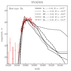
a)

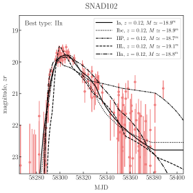
b)

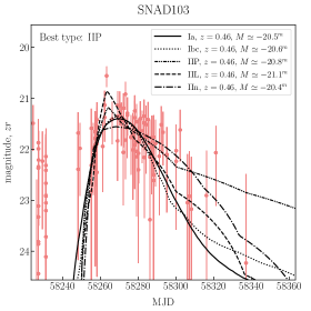
c)

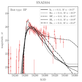
d)

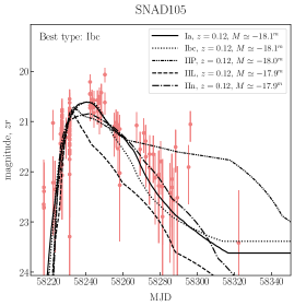
e)

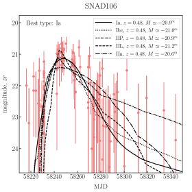
f)

Figure 13: Light curves of SNAD supernova candidates in $zr$-band and the results of their fit by Nugent’s supernova models.

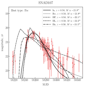
a)

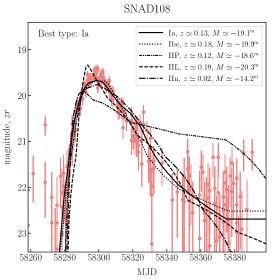
b)

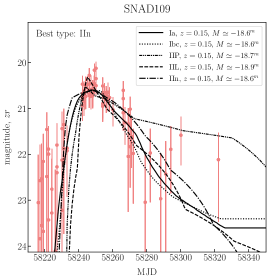
c)

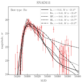
d)

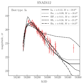
e)

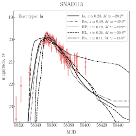
f)

Figure 14: Light curves of SNAD supernova candidates in $zr$-band and the results of their fit by Nugent’s supernova models.

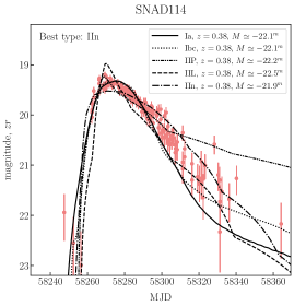
a)

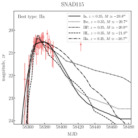
b)

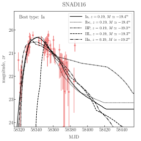
c)

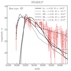
d)

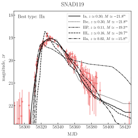
e)

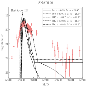
f)

Figure 15: Light curves of SNAD supernova candidates in $zr$-band and the results of their fit by Nugent’s supernova models.

a)

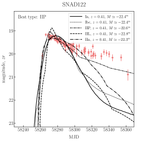
b)

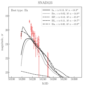
c)

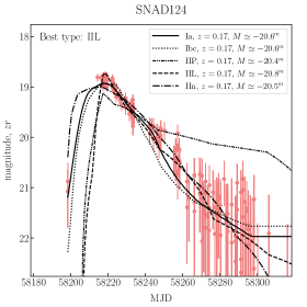
d)

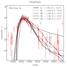
e)

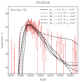
f)

Figure 16: Light curves of SNAD supernova candidates in $zr$-band and the results of their fit by Nugent’s supernova models.

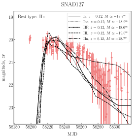
a)

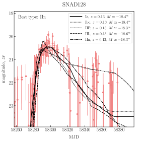
b)

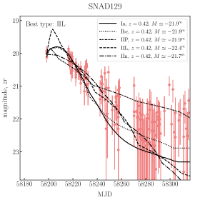
c)

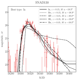
d)

e)

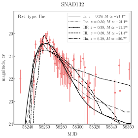
f)

Figure 17: Light curves of SNAD supernova candidates in $zr$-band and the results of their fit by Nugent’s supernova models.

a)

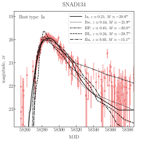
b)

c)

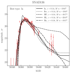
d)

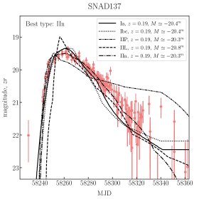
e)

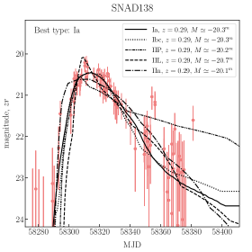
f)

Figure 18: Light curves of SNAD supernova candidates in $zr$-band and the results of their fit by Nugent’s supernova models.

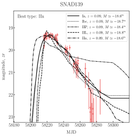
a)

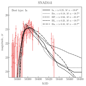
b)

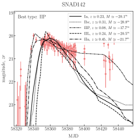
c)

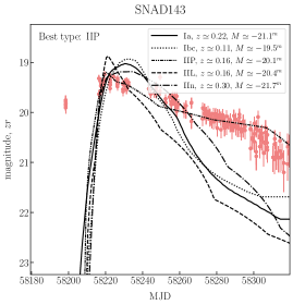
d)

e)

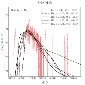
f)

Figure 19: Light curves of SNAD supernova candidates in $zr$-band and the results of their fit by Nugent’s supernova models.

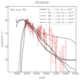
a)

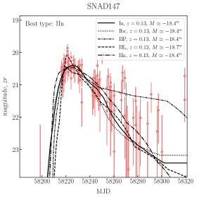
b)

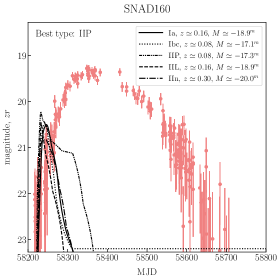
c)

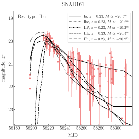
d)

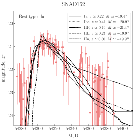
e)

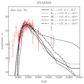
f)

Figure 20: Light curves of SNAD supernova candidates in $zr$-band and the results of their fit by Nugent’s supernova models.

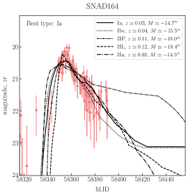
a)

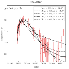
b)

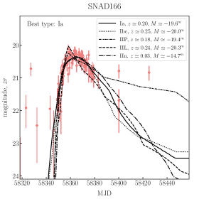
c)

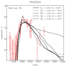
d)

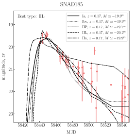
e)

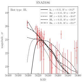
f)

Figure 21: Light curves of SNAD supernova candidates in $zr$-band and the results of their fit by Nugent’s supernova models.

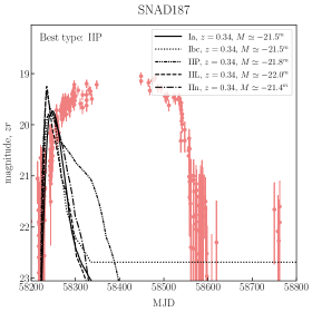
a)

b)

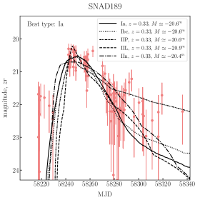
c)

Figure 22: Light curves of SNAD supernova candidates in $zr$-band and the results of their fit by Nugent’s supernova models.

Appendix C SNAD ZTF viewer

We present below a glimpse on the expert’s session of the SNAD viewer (Malanchev 2021b; Malanchev et al. 2022).