$k$-Dimensional Agreement in Multiagent Systems for Distributed Coordination

Abstract

Given a network of agents, each characterized by an initial scalar value, we study the problem of designing distributed linear algorithms such that the agents agree in a generalized sense on a vector quantity that belongs to a $k$-dimensional subspace. This problem is motivated by applications in distributed computing and sensing, where agents seek to simultaneously evaluate $k$ independent functions at a common vector point by running a single distributed algorithm. We show that linear protocols can agree only on quantities that are oblique projections of the vector of initial conditions, and we provide an algebraic characterization of all agreement protocols that are consistent with a certain communication graph. By leveraging this characterization, we propose a design procedure for constructing agreement protocols, and we investigate what are the structural properties of communication networks that can reach an agreement on arbitrary weights. More broadly, our results show that agreement algorithms are capable of simultaneously solving $k$ consensus problems at a fraction of the communication volume and space complexity of classical algorithms but, in general, require higher network connectivity. The applicability of the framework is illustrated via simulations on two problems in robotic formation and distributed regression.

1 Introduction

Coordination and consensus protocols are central to many network synchronization problems, including rendezvous, distributed convex optimization, and distributed computation and sensing. One of the most established distributed coordination algorithms is that of consensus, whereby the states of a group of agents asymptotically converge to a unique common value that is a weighted average of the initial agents’ states (see, for example, the representative works [1, 2, 3]). On the other hand, in several applications, it is instead of interest to compute asymptotically multiple weighted averages of the initial states. Relevant examples where this problem is of interest include distributed computation [4, 5], where the weighting accounts for different desired outcomes, task allocation algorithms [6], where weights account for heterogeneous computational capabilities, distributed sensing [7, 8], where the weighting is proportional to the accuracy of each sensing device, and robotic formation [9], where one agent would like to achieve a certain configuration relative to another agent.

Mathematically, given a vector $x_{0}\in\mathbb{R}^{n}$ of initial states or estimates – such that each of its entries is known only locally by one agent – and a rank-$k$ matrix $W\in\mathbb{R}^{n\times n}$ describing the desired asymptotic weights, we say that the group reaches a $k$-dimensional agreement when, asymptotically, the agents’ states converge to $Wx_{0}$. The goal of this paper is to design distributed control protocols that enable the set of agents to reach a $k$-dimensional agreement on a given $W$.

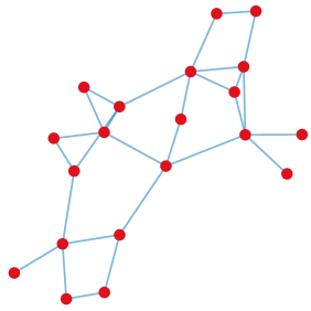
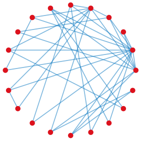
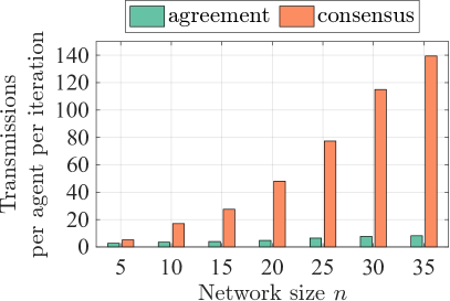
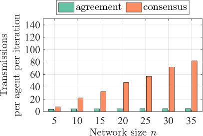
Figure 1: Communication complexity of running $k$ consensus algorithms in parallel vs one $k$-dimensional agreement algorithm (proposed in this paper) to compute $k=\left\lfloor\frac{n}{2}\right\rfloor$ weighted average means of a global quantity. (a) and (c) Erdős–Rényi network model. (b) and (d) Barabasi-Albert model. Bars denote the average number of transmissions per iteration per agent. See Section 4.2.

A natural approach to tackle this problem consists in executing $k$ consensus algorithms [2] in parallel, each designed to converge to a specific row of $Wx_{0}$. Unfortunately, the communication and computational complexities of such an approach do not scale with the network size, thus, our objective here is to reach agreement by running a single distributed algorithm. A comparison of the communication load involved by $k$ parallel consensus algorithms and the proposed $k$-dimensional agreement method is exemplified in Fig. 1 (simulation details are provided in Section 3.2).

Related work. The agreement problem studied in this work stems from that of consensus. Because of their centrality, consensus algorithms have been extensively studied in the literature. A list of representative topics (necessarily incomplete) includes: sufficient and/or necessary conditions to reach a consensus [10, 11, 2, 12, 13, 14], time delays [12], consensus with linear objective maps [15], the use of the alternating direction method of multipliers (ADMM) [16, 17, 18], convergence rates [19, 20], and robustness investigations [21, 22]. Differently from constrained consensus problems [23, 24], where the agents’ states must satisfy agent-dependent constraints during transients and the asymptotic value lies in the intersection of the constraint sets, in our setting the values are instead constrained at convergence, and thus state of the agents may not converge to identical values. In Pareto optimal distributed optimization [25], the group of agents cooperatively seeks to determine the minimizer of a cost function that depends on agent-dependent decision variables. Clustering-based consensus [26, 27, 28] is a closely-related problem where the states of agents in the same cluster of the graph converge to identical values, while inter-cluster states can differ. Differently from this setting, which is obtained by using weakly-connected communication graphs to separate the state of different communities, here we are interested in cases where the asymptotic state of each agent depends on every other agent in the network. To the best of our knowledge, agreement problems exhibiting this dependence where the agents’ states do not converge to identical values have not been studied. A relevant exception is the problem of scaled consensus considered in [29], where agents agree on subspaces of dimension $k=1$. In this paper, we tackle the more general problem $k\geq 1$; as shown shortly below, the extension to $k>1$ is non-trivial since standard assumptions made for consensus are not sufficient to guarantee agreement (see Example 4.10).

Contributions. The contribution of this work is fourfold. First, we formulate the $k$-dimensional agreement problem, we propose the use of linear control protocols for this purpose, and we discuss the fundamental limitations of these protocols in solving agreement problems. More precisely, we show that linear protocols can converge asymptotically to vector points that are oblique projections of the vector of initial estimates. Conversely, we also show that for any given oblique projection, there exists a linear protocol that emulates that linear operator, provided that the underlying communication graph is sufficiently connected. Second, for a pre-specified communication graph, we provide an algebraic characterization of all agreement protocols that are consistent with this graph. We show how such characterization can be used to design efficient numerical algorithms for agreement. Third, we provide graph-theoretic conditions to check whether a graph can sustain agreement dynamics. Our conditions demonstrate that widely-adopted graphs, such as the line and circulant topologies, can reach agreement on subspaces of dimension at most $k=1$, thus suggesting that higher connectivity is required for agreement reachability on high-dimensional subspaces. Moreover, our analysis shows that agreement is made possible graph-theoretically by the presence of Hamiltonian decompositions in the communication graph. Fourth, we show that agreement algorithms can be adapted to account for cases where the local estimates are time-varying and, in this case, we prove convergence of these algorithms in the form of an input-to-state stability-type bound. Finally, we illustrate the applicability of the framework on regression and robotic coordination problems through simulations.

Organization. Section 2 introduces necessary concepts, Section 3 formalizes the problem, Section 4 studies agreement protocols over complete graphs, Section 5 illustrates our algebraic characterization of agreement protocols and illustrates numerical methods to compute agreement algorithms, Section 6 provides graph-theoretic conditions for agreement. Section 7 extends the approach to tracking problems and Section 8 illustrates the techniques via numerical simulations. Conclusions and directions are discussed in Section 9.

2 Preliminaries

We first introduce some basic notions used in the paper.

Notation. We denote by $\mathbb{N}_{>0}=\{1,2,\dots\}$ the set of positive natural numbers, by $\mathbb{C}$ the set of complex numbers, and by the set of real numbers. Given $x\in\mathbb{C}$, $\Re(x)$ and $\Im(x)$ denote its real and imaginary parts, respectively. Given vectors $x\in{}^{n}$ and $u\in{}^{m}$, we let $(x,u)\in{}^{n+m}$ denote their concatenation. We denote by $\mathds{1}_{n}\in{}^{n}$ the vector of all ones, by $I_{n}\in{}^{n\times n}$ the identity matrix, by $\mymathbb{0}_{n,m}\in{}^{n\times m}$ the matrix of all zeros (subscripts are dropped when dimensions are clear from the context). Given $A\in{}^{n\times n}$, we denote its spectrum by $\sigma(A)=\{\lambda\in\mathbb{C}\;:\;\det(\lambda I-A)=0\}$, and by ${\lambda}_{\textup{max}}\left(A\right)=\max\{\Re(\lambda)\;:\;\lambda\in\sigma(A)\}$ its spectral abscissa; also, we use the notation $A=[a_{ij}]$, where $a_{ij}$ is the element in row $i$ and column $j$ of $A$. Given $A\in{}^{n\times m}$, $\operatorname{Im}(A)$ and $\ker(A)$ denote its image and null space, respectively. Given a polynomial with real coefficients $p(\lambda)=\lambda^{n}+p_{1}\lambda^{n-1}+\dots+p_{n}$, $p(\lambda)$ is stable if all its roots have negative real part.

Graph-theoretic notions. A directed graph (abbreviated digraph), denoted by $\mathcal{G}=(\mathcal{V},\mathcal{E})$, consists of a set of nodes $\mathcal{V}=\{1,\dots,n\}$ and a set of directed edges $\mathcal{E}\subseteq\mathcal{V}\times\mathcal{V}$. An element $(i,j)\in\mathcal{E}$ denotes a directed edge from node $j$ to $i$. We will often use the notion of weighted digraph $\mathcal{G}=(\mathcal{V},\mathcal{E},A)$, where $A\in{}^{n\times n}$ is the graph’s adjacency matrix; $A=[a_{ij}]$ satisfies $a_{ij}\neq 0$ only if $(i,j)\in\mathcal{E}$ and $a_{ij}=0$ if $(i,j)\not\in\mathcal{E}$. More generally, for fixed $\mathcal{G}$ and $A\in{}^{n\times n}$, we say that $A$ is consistent with $\mathcal{G}$ if $A$ has the zero-nonzero pattern of an adjacency matrix for $\mathcal{G}$. The set of (in)neighbors of $i\in\mathcal{V}$ is $\mathcal{N}_{i}=\{j\in\mathcal{V}\setminus\{i\}\;:\;(i,j)\in\mathcal{E}\}$. A graph is complete if there exists an edge connecting every pair of nodes, and is sparse otherwise. A path in $\mathcal{G}$ is a sequence of edges $(e_{1},e_{2},\dots)$, $e_{j}\in\mathcal{E}$ for all $j=1,2,\dots$, such that the initial node of each edge is the final node of the preceding edge. Notice that a path may contain repeated edges and, also, going along the path one may reach repeated nodes. The length of a path is the number of edges contained in the sequence $(e_{1},e_{2},\dots)$. A graph is strongly connected if, for any $i,j\in\mathcal{V}$, there is a directed path from $i$ to $j$. A closed path is a path whose initial and final vertices coincide. A closed path is a cycle if, going along the path, one reaches no node, other than the initial-final node, more than once. A cycle of length equal to one is a self cycle. The length of a cycle is equal to the number of edges in that cycle; notice that, because nodes cannot be repeated, the length of a cycle is equal to the number of nodes encountered along the cycle. A set of node-disjoint cycles such that the sum of the cycle lengths is equal to $\ell$ is called a Hamiltonian $\ell$-decomposition (or cycle family of length $\ell$). See Fig. 2 for illustration.

Structural analysis and sparse matrix spaces. We rely on the structural approach to system theory proposed in [30, 31]. We are concerned with linear subspaces obtained by forcing certain entries of the matrices in ^n×n to be zero. More precisely, given a digraph $\mathcal{G}$, we define $\mathcal{A}_{\mathcal{G}}$ to be the vector space in ^n×n that contains all matrices that are consistent with $\mathcal{G}$, and whose nonzero entries are independent parameters. The vector space $\mathcal{A}_{\mathcal{G}}$ can be represented by a $n\times n$ structure matrix $\mathbf{A}_{\mathcal{G}}$, whose entries are either algebraically independent parameters in (denoted by ✻) or fixed zeros (denoted by $0$). We define a vector of parameters $a=(\{a_{ij}\}_{(i,j)\in\mathcal{E}})$ such that $\mathbf{A}_{\mathcal{G}}(a)$ defines a numerical realization of the structured matrix $\mathbf{A}_{\mathcal{G}}$, namely, $\mathbf{A}_{\mathcal{G}}(a)\in\mathcal{A}_{\mathcal{G}}$. For instance, for the graph in Figure 2, we have

$$\mathbf{A}_{\mathcal{G}} =\begin{bmatrix}\text{\char 91}&0&\text{\char 91}&0\\ \text{\char 91}&0&\text{\char 91}&0\\ 0&\text{\char 91}&0&\text{\char 91}\\ 0&\text{\char 91}&0&0\\ \end{bmatrix},\mathbf{A}_{\mathcal{G}}(a)=\begin{bmatrix}a_{11}&0&a_{13}&0\\ a_{21}&0&a_{23}&0\\ 0&a_{32}&0&a_{34}\\ 0&a_{42}&0&0\\ \end{bmatrix},$$

where $a=(a_{11},a_{13},a_{21},a_{23},a_{32},a_{34},a_{42})$.

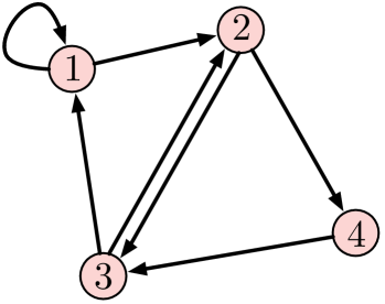
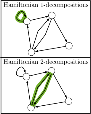
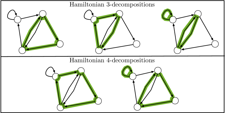
Figure 2: (a) Illustration of a digraph and (b)-(c) associated Hamiltonian $\ell$-decompositions, $\ell\in\{1,\dots,4\}$ (a Hamiltonial $\ell$-decomposition is a set of node-disjoint cycles such that the sum of the cycle lengths is equal to $\ell$ ).

Projections and linear subspaces. We next recall some basic notions regarding projections in linear algebra (see, e.g., [32]). Two vectors $x,y\in{}^{n}$ are orthogonal if $x^{\mathsf{T}}y=0$; the orthogonal complement of $\mathcal{M}\subset{}^{n}$ is a linear subspace defined as $M^{\bot}:=\{x\in{}^{n}\;:\;x^{\mathsf{T}}y=0,\,\forall~{}y\in\mathcal{M}\}$. Given two subspaces $\mathcal{M},\mathcal{N}\subseteq{}^{n}$, the subspace $\mathcal{W}\subseteq{}^{n}$ is a direct sum of $\mathcal{M}$ and $\mathcal{N}$, denoted $\mathcal{W}=\mathcal{M}\oplus\mathcal{N}$, if $\mathcal{M}\cap\mathcal{N}=\{0\}$, and $\mathcal{M}+\mathcal{N}=\{u+v\;:\;u\in\mathcal{M},v\in\mathcal{N}\}=\mathcal{W}$. The subspaces $\mathcal{M},\mathcal{N}\subset{}^{n}$ are complementary if $\mathcal{M}\oplus\mathcal{N}={}^{n}$. A matrix $\Pi\in{}^{n\times n}$ is called a projection in ^n×n if $\Pi^{2}=\Pi$. Given complementary subspaces $\mathcal{M},\mathcal{N}\subset{}^{n}$, for any $z\in{}^{n}$ there exists a unique decomposition of the form $z=x+y$, where $x\in\mathcal{M}$, $y\in\mathcal{N}$. The transformation $\Pi_{\mathcal{M},\mathcal{N}}$, defined by $\Pi_{\mathcal{M},\mathcal{N}}z:=x$, is called projection onto $\mathcal{M}$ along $\mathcal{N}$, and the transformation $\Pi_{\mathcal{N},\mathcal{M}}$ defined by $\Pi_{\mathcal{N},\mathcal{M}}z:=y$ is called projection onto $\mathcal{N}$ along $\mathcal{M}$. Moreover, the vector $x$ is the projection of $z$ onto $\mathcal{M}$ along $\mathcal{N}$, and the vector $y$ is the projection of $z$ onto $\mathcal{N}$ along $\mathcal{M}$. The projection $\Pi_{\mathcal{M},\mathcal{M}^{\bot}}$ onto $\mathcal{M}$ along $\mathcal{M}^{\bot}$ is called orthogonal projection onto $\mathcal{M}$. Because the subspace $\mathcal{M}$ uniquely determines $\mathcal{M}^{\bot}$, in what follows we will denote $\Pi_{\mathcal{M},\mathcal{M}^{\bot}}$ in compact form as $\Pi_{\mathcal{M}}$. General projections that are not orthogonal are called oblique projections. We recall the following instrumental results.

Lemma 2.1

(See [32, Thm. 2.11 and Thm. 2.31]) If $\Pi\in{}^{n\times n}$ is a projection with $\operatorname{rank}\left(\Pi\right)=k$, then there exists an invertible matrix $T\in{}^{n\times n}$ such that

$$\Pi=T\begin{bmatrix}I_{k}&0\\ 0&0\end{bmatrix}T^{\scalebox{0.75}[0.9]{$-$}1}.$$

Moreover, if $\Pi$ is an orthogonal projection, then $T$ can be chosen to be an orthogonal matrix, i.e., $TT^{\mathsf{T}}=I$. $\square$

Lemma 2.2

(See [32, Thm. 2.26]) Let $\mathcal{M},\mathcal{N}$ be complementary subspaces and let the columns of $M\in{}^{n\times k}$ and $N\in{}^{n\times k}$ form a basis for $\mathcal{M}$ and $\mathcal{N}^{\bot}$, respectively. Then $\Pi_{\mathcal{M},\mathcal{N}}=M(N^{\mathsf{T}}M)^{\scalebox{0.75}[0.9]{$-$}1}N^{\mathsf{T}}$. $\square$

Recall the following known properties [32, Thm. 1.60]:

$$\operatorname{Im}(M^{\mathsf{T}}) =\operatorname{Im}(M^{\dagger})=\operatorname{Im}(M^{\dagger}M)=\operatorname{Im}(M^{\mathsf{T}}M),$$

$$\ker(M) =\operatorname{Im}(M^{\mathsf{T}})^{\bot}=\ker(M^{\dagger}M)=\operatorname{Im}(I-M^{\dagger}M).$$

From these properties, it follows from Lemma 2.2 that if $M\in{}^{m\times n}$, then $\Pi_{\operatorname{Im}(M)}=MM^{\dagger}$ and $\Pi_{\ker(M)}=I-M^{\dagger}M$, where $M^{\dagger}\in{}^{n\times m}$ is the Moore-Penrose inverse of $M$.

3 Problem Setting

In this section, we formalize the problem and discuss a set of applications to show its relevance for distributed computation.

3.1 Problem formulation

Consider $n$ agents whose communication topology is described by a digraph $\mathcal{G}=(\mathcal{V},\mathcal{E})$, $\mathcal{V}=\{1,\dots,n\}$, and let $x_{i}\in\real$ denote the state of the $i$-th agent, $i\in\mathcal{V}$. We are interested in a model where each agent exchanges its state with its neighbors and updates it using the following dynamics:

$$\dot{x}_{i} =a_{ii}x_{i}+\sum_{j\in\mathcal{N}_{i}}a_{ij}x_{j}, \forall\,\,i\in\mathcal{V},$$ (1)

where $a_{ij}\in\real$, $(i,j)\in\mathcal{E}$, is a weighting factor. Setting $A=[a_{ij}]$ with $a_{ij}=0$ if $(i,j)\not\in\mathcal{E}$, and $x=(x_{1},\dots,x_{n})$, the dynamics can be written in vector form as:

$$\dot{x}=Ax.$$ (2)

We say that the network dynamics (2) reaches a $k$-dimensional agreement if, asymptotically, each state variable converges to an (agent-dependent) weighted sum of the initial conditions, such that the value at convergence is confined to a subspace of dimension $k$. We formalize this notion next.

Definition 3.1

($k$-dimensional agreement) Let $W\in{}^{n\times n}$ be such that $\operatorname{rank}\left(W\right)=k\in\mathbb{N}_{>0}$. We say that the update (2) globally asymptotically reaches a $k$-dimensional agreement on $W$ if, for any $x(0)\in{}^{n}$,

$$\lim_{t\rightarrow\infty}x(t)=Wx(0).$$ (3)

$\square$

Definition 3.1 formalizes a notion of agreement between the agents where the asymptotic network state is a vector that belongs to the $k$-dimensional space $\operatorname{Im}(W)$. Remarkably, agreement generalizes the well-studied notion of consensus, see Remark 3.2 below. Notice that agreement does not necessarily imply that the agents’ state variables coincide asymptotically: in fact, $\lim_{t\rightarrow\infty}\|x_{i}(t)-x_{j}(t)\|=0$ only holds if all rows of $W$ are identical. In this sense, agreement should be interpreted as a generalized notion of consensus, where state variables agree within a $k$-dimensional subspace. As we illustrate below, this generalization is particularly useful to engineer the simultaneous computation of multiple quantities of interest in multi-agent coordination scenarios.

Remark 3.2

(Relationship with consensus problems) In the special case $k=1$, $W$ can be written as $W=vw^{\mathsf{T}}$ for some $v,w\in{}^{n}$. This corresponds to the problem of scaled consensus, studied in [29]. When, in addition, $v=\mathds{1}$ and $w^{\mathsf{T}}\mathds{1}=1$, we recover the classical consensus problem, see, e.g., [2]. When, $v=\mathds{1}$ and $w=\frac{1}{n}\mathds{1}$, our problem simplifies to average consensus [2, Sec. 2]. Importantly, notice that all state variables converge to the same quantity (namely, $\lim_{t\rightarrow\infty}\|x_{i}(t)-x_{j}(t)\|=0$) if and only if $v=\mathds{1}.$ $\square$

In line with the consensus literature, it is natural to distinguish between agreement problems on some subspace and agreement problems on arbitrary subspaces.

Definition 3.3

(Agreement on some vs arbitrary weights) Let $k\in\mathbb{N}_{>0}$ be a given constant.

• The set of agents is said to be globally $k$-agreement reachable on some weights if there exists $A\in{}^{n\times n},$ such that (2) globally asymptotically reaches an agreement on some $W\in{}^{n\times n}$ with $\operatorname{rank}\left(W\right)=k.$

• The set of agents is said to be globally $k$-agreement reachable on arbitrary weights if, for any $W\in{}^{n\times n}$ with $\operatorname{rank}\left(W\right)=k,$ there exists $A$ such that (2) globally asymptotically reaches a $k$-dimensional agreement on $W$.

  $\square$

It is immediate to see that if a set of agents is globally agreement reachable on arbitrary weights, then it is also globally agreement reachable on some weights; however, the inverse implication does not hold in general. We illustrate the differences between the two notions in the following example.

Example 3.4

(Comparison between reachability on arbitrary and some weights) Consider a set of agents whose communication graph is a set of isolated nodes (i.e., $\mathcal{V}=\{1,\dots,n\}$ and $\mathcal{E}=\{\}$). The set of protocols (2) compatible with this graph is $A=\operatorname{diag}(a_{1},\dots,a_{n});$ notice that $\lim_{t\rightarrow\infty}x(t)=\lim_{t\rightarrow\infty}e^{At}x(0)$ exists if and only if $\max\{a_{i}\}_{i\in\{1,\dots,n\}}\leq 0.$ When the latter condition holds, $\lim_{t\rightarrow\infty}e^{At}=\operatorname{diag}(d_{1},\dots,d_{n}),$ where $d_{i}=0$ if $a_{i}<0$ and $d_{i}=1$ otherwise. Hence, the agents are globally agreement reachable on some weights (precisely, $W=\operatorname{diag}(d_{1},\dots,d_{n})$), but are not globally agreement reachable on arbitrary weights (e.g., any non-diagonal $W$). $\square$

We note that the notion of agreement reachability on some weights generalizes that of consensus reachablity [33], while agreement reachability on arbitrary weights generalizes that of global average consensus reachablity [34].

In many distributed computing problems (see Section 3.2 for a discussion), it is of interest to pre-specify a certain $W$ and to design a protocol $A$ that achieves (2). Motivated by this framework, we formalize the following two problems.

Problem 1

(Construction of communication graphs for agreement) Let $k\in\mathbb{N}_{>0}.$ Determine the largest class of communication graphs that guarantees that the set of agents is globally $k$-agreement reachable on arbitrary weights. $\square$

Problem 2

(Agreement protocol design) Let $W\in{}^{n\times n}$ be a given matrix such that $\operatorname{rank}\left(W\right)=k\in\mathbb{N}_{>0}$ and let $\mathcal{G}$ be a communication graph as in Problem 1. Determine a matrix $A$, consistent with $\mathcal{G},$ such that (3) holds with maximum rate of convergence. $\square$

An important distinction between the two problems is in order. Problem 1 is a feasibility problem: it asks to determine the class of communication structures that enable the agents to be globally agreement reachable on arbitrary weights. Problem 2 instead is a protocol design problem: it asks to determine a realization of $A$ that enables the agents to reach an agreement on a pre-specified $W,$ given that the communication structure is fixed. We conclude this section by discussing an important technical challenge related to solving agreement problems as opposed to classical consensus problems.

Remark 3.5

(New technical challenges with respect to consensus) Several techniques have been proposed in the literature to design consensus protocols, including Laplacian-based methods [2], distributed weight design [35], and centralized weight design [20]. However, all these methods critically rely on the assumption that the consensus protocol $A$ is a non-negative matrix and on the Perron-Frobenius Theorem [36]. Unfortunately, the Perron-Frobenius theory, a central piece of consensus weight design techniques, no longer applies to $k$-agreement protocols for two reasons: (i) the entries of $W$ are possibly negative scalars and (ii) agreement protocols can no longer be restricted to matrices with a single dominant eigenvalue (see Lemma 4.1 shortly below). Hence, the agreement problem formalized here presents new theoretical challenges that require the development of new tools for the analysis. $\square$

3.2 Illustrative scenarios

In this section, we present some illustrative applications where the agreement problem emerges naturally in practice.

Distributed parallel computation of multiple functions. Many numerical computational tasks amount to evaluating a certain function at a given point [37]. Relevant examples include computing scalar addition, inner products, matrix addition and multiplication, matrix powers, finding the least prime factor, etc. [37, Sec. 1.2.3]. Formally, given a function $f:{}^{n}\rightarrow\real$ and an input point $(\hat{x}_{1},\dots,\hat{x}_{n})$, the objective is then to evaluate $f(\hat{x}_{1},\dots,\hat{x}_{n});$ a common solution to this problem amounts to the design of an iterative algorithm of the form $\dot{x}=g(x)$ such that $\lim_{t\rightarrow\infty}x(t)=f(\hat{x}_{1},\dots,\hat{x}_{n}).$

Further, in many cases, the computing task naturally has a distributed nature [38], where each quantity $\hat{x}_{i}$ is known only locally by agent $i,$ and it is often of interest to maintain $\hat{x}_{i}$ private from the rest of the network; in these cases, the distributed computation literature (see, e.g., [38]) has proposed update rules of the form $\dot{x}_{i}=g_{i}(x),$ to be designed such that, $\forall i,$ $\lim_{t\rightarrow\infty}x_{i}(t)=f(\hat{x}_{1},\dots,\hat{x}_{n}).$

Extending these classical frameworks, consider now the problem of evaluating, in a distributed fashion, several functions simultaneously. Formally, given $n$ functions $f_{1},\dots,f_{n}:{}^{n}\rightarrow\real$ and an input point $(\hat{x}_{1},\dots,\hat{x}_{n}),$ the objective is to design distributed protocols of the form $\dot{x}_{i}=g_{i}(x)$ such that the state of each agent converges to

$$\lim_{t\rightarrow\infty}x_{i}(t)=f_{i}(\hat{x}_{1},\dots,\hat{x}_{n}), \forall i.$$ (4)

Importantly, this problem is relevant in computing tasks where one would like to evaluate several functions by running a single distributed algorithm; examples include computing weighted scalar additions (with agent-dependent weights) and weighted inner products, to name a few [37, Sec. 1.2.3].

Assuming that functions $f_{i}(\cdot)$ to be evaluated are linear, namely, $f_{i}(x)=w_{i}^{\mathsf{T}}x$, with $w_{i}\in{}^{n}$, $w_{i}^{\mathsf{T}}\mathds{1}=1$, and that $k$ vectors of $\{w_{1},\dots,w_{n}\}$ are linearly independent it is natural to consider two approaches to solve this problem.

(Approach 1) A first approach consists of running $k$ independent consensus algorithms [34] in parallel, as outlined next. Let each agent $i\in\mathcal{V}$ replicate its state $k$ times, yielding $\{x_{i}^{(d)}\in\real\}_{d\in\{1,\dots,k\}},$ and let each state be updated using the following protocol:

$$\dot{x}_{i}^{(d)}=\sum_{j\in\mathcal{N}_{i}}a_{ij}^{(d)}(x_{j}^{(d)}-x_{i}^{(d)}), \dot{x}_{i}^{(d)}(0)=\hat{x}_{i},$$

By letting $A^{(d)}=[a_{ij}^{(d)}],$ and by choosing the weights such that $w_{d}^{\mathsf{T}}A^{(d)}=0,$ it is well-known [34, Thm. 1] that this Laplacian-based consensus algorithm satisfies

$$\lim_{t\rightarrow\infty}x^{(d)}_{i}(t)=w_{d}^{\mathsf{T}}\hat{x}, d\in\{1,\dots,k\},$$

provided that the communication graph is strongly connected. Namely, the $d$-th state replica of each agent achieves (4).

Unfortunately, it is immediate to see that the spatial and communication complexities of this approach do not scale well with $n$: each agent must maintain $k$ replica scalar state variables and, at every time step, each agent must transmit these $k$ variables to all its neighbors. It follows that the per-agent spatial complexity is $\mathcal{O}(k)$ (since each agent maintains $k$ copies of a scalar state variable), and the per-agent communication complexity is $\mathcal{O}(k\cdot\text{deg}(\mathcal{G}))$ (and thus $\mathcal{O}(n\cdot\text{deg}(\mathcal{G}))$ when $k$ is proportional to $n$). Here, $\text{deg}(\mathcal{G})$ denotes the largest in/out node degree in $\mathcal{G}$.

(Approach 2) To overcome the scalability issue of (Approach 1), it is natural to consider the adoption of a single protocol of the form (2) and to design matrix $A$ such that (3) holds with $W=[w_{1},\dots,w_{n}]^{\mathsf{T}}$. Techniques to design such $A$ are the focus of this work and will be discussed shortly below in Section 5. In this case, the per-agent spatial complexity is $\mathcal{O}(1)$ since agents maintain a single scalar state variable, and the communication complexity is $\mathcal{O}(\text{deg}(\mathcal{G}))$. A comparison of the communication volumes of the two approaches is illustrated in Fig. 1. It is worth noting the fundamental difference between the two considered approaches: in (Approach 1), one compputes $k$ independent quantities by running $k$ distributed averaging algorithms, in (Approach 2) one can compute the $k$ independent quantities by running a single distributed algorithm.

Constrained Kalman filtering. Kalman filters are widely used tools to estimate the states of a dynamic system. In constructing Kalman filters, one often faces the challenge of accounting for state-constrained dynamic systems; examples include camera tracking, fault diagnosis, chemical processes, vision-based systems, and biomedical systems [39]. Formally, given a dynamic system of the form $\dot{x}=Fx+Bu+w,$ $y=Cx+e,$ with state constraint $Dx=0,$ (see [39, eq. (10)]) where $x$ is the state vector, $u$ is a known input, $y$ is the measurement, and $w$ and $e$ are stochastic noise inputs, $F,B,C,D$ are matrices of suitable dimensions, the objective is that of constructing an optimal estimate $\hat{x}^{c}$ of $x$ given past measurements $\{y(\tau),\tau\leq t\}.$ Denoting by $\hat{x}^{u}$ the state estimate constructed using an unconstrained Kalman filter, a common approach to tackle the constrained problem consists of projecting $\hat{x}^{u}$ onto the constraint space [39, Sec. 2.3]:

$$\hat{x}^{c}=\arg\min_{x}~{}~{} (x-\hat{x}^{u})^{\mathsf{T}}Q(x-\hat{x}^{u})$$

s.t. $$Dx=0,$$

where $Q$ is a positive definite matrix. The solution to this problem is $\hat{x}^{c}=(I-Q^{\scalebox{0.75}[0.9]{$-$}1}D^{\mathsf{T}}(DQ^{\scalebox{0.75}[0.9]{$-$}1}D^{\mathsf{T}})^{\scalebox{0.75}[0.9]{$-$}1}D)\hat{x}^{u};$ notice that this is an oblique projection of the vector $\hat{x}^{u}.$ To speed-up the calculation, it is often of interest to parallelize the computation of $\hat{x}^{c}$ across a group of distributed processors. It is then immediate to see that the agreement framework (3) provides a natural solution to this problem.

Robotic formation control. A common objective in robotic formation problems is that of promoting cohesion between certain groups of robots in such a way that robots in the same group behave similarly. Consider a group of $n=4$ robots modeled through single-integrator dynamics. Let $x\in{}^{4}$ denote the $x$-coordinates of the group positions (we refer to Section 8 for a two-dimensional example with additional details), and assume that the group is interested in achieving a final formation $x$ that minimizes the control energy and such that $x_{1}=x_{2}$ and $x_{3}=x_{4},$ but not necessarily $x_{1}=x_{3}.$ Further, because each robot has no knowledge of global coordinates, this must be achieved by exchanging local coordinates only. These formation objectives can be encapsulated by constraining the final state as $Dx=0,$ where

$$D=\begin{bmatrix}1&-1&0&0\\ 0&0&1&-1\end{bmatrix}.$$

Matrix $D$ allows here to encode “attraction forces” between pairs of robots. It is immediate to see that this problem can be tackled by leveraging the agreement framework (3).

4 Characterization of the agreement space and fundamental limitations

In this section, we study the properties of the agreement space for linear protocols, cf. (2) and, as a result, identify some fundamental limitations regarding the possible weight matrices. Regarding Problem 1, this (i) allows us to provide an answer for complete digraphs and (ii) identify necessary conditions on connectivity for general digraphs.

4.1 Algebraic characterization of agreement space

We provide here a characterization of the agreement space for (2) and build on it to construct a matrix $A$ that defines an agreement protocol over the complete graph. We begin with the following instrumental result.

Lemma 4.1

(Spectral properties of agreement protocols) The set of agents is globally $k$-agreement reachable on some weights if and only if there exists a nonsingular $T\in{}^{n\times n}$ such that $A$ admits the following decomposition:

$$A=T\begin{bmatrix}\mymathbb{0}_{k,k}&\mymathbb{0}_{k,n-k}\\ \mymathbb{0}_{n-k,k}&B\end{bmatrix}T^{\scalebox{0.75}[0.9]{$-$}1},$$ (5)

where $B\in{}^{(n-k)\times(n-k)}$ satisfies ${\lambda}_{\textup{max}}\left(B\right)<0$. $\square$

Proof 4.2.

(If) When (5) holds, we have that:

$$\lim_{t\rightarrow\infty}x(t)=\lim_{t\rightarrow\infty}e^{At}x(0)=\underbrace{T\begin{bmatrix}I_{k}&\mymathbb{0}\\ \mymathbb{0}&\mymathbb{0}\end{bmatrix}T^{\scalebox{0.75}[0.9]{$-$}1}}_{:=W}x(0)=Wx(0).$$

(Only if) From [36, Lemma 1.7], if $\lim_{t\rightarrow\infty}e^{At}$ exists, then ${\lambda}_{\textup{max}}\left(A\right)\leq 0$; moreover, if $\lambda$ is an eigenvalue of $A$ such that $\Re(\lambda)=0$, then $\lambda=0$ and its algebraic and geometric multiplicities coincide. It follows that $A$ must satisfy (5).

Lemma 4.1 shows that matrices $A$ that characterize agreement protocols satisfy two properties: (i) their spectrum is $\sigma(A)=\{0\}\cup\{\lambda_{1},\dots,\lambda_{n-k}\}$, $\Re(\lambda_{i})<0$, and (ii) the eigenvalue at the origin has identical algebraic and geometric multiplicities, which are equal to $k$. Although the lemma establishes a condition for agreement on some weights, a direct application of Definition 3.3 allows us to derive the following necessary condition for agreement on arbitrary weights.

Corollary 4.3.

If a set of agents is globally $k$-agreement reachable on arbitrary weights, then (5) holds. $\square$

In the following result, we characterize the class of weight matrices $W$ on which an agreement can be reached.

Proposition 4.4.

(Characterization of agreement space) Let $x(t)$ denote the solution of (2) with initial condition $x(0)$. If $\lim_{t\rightarrow\infty}x(t):=x_{\infty}$ exists, then there exist complementary subspaces $\mathcal{M},\mathcal{N}\subset{}^{n}$ such that $x_{\infty}=\Pi_{\mathcal{M},\mathcal{N}}x(0).$ Moreover, let $\{t_{1},\dots,t_{k}\}$ denote the first $k$ columns of $T$ in (5) and $\{\tau_{1}^{\mathsf{T}},\dots,\tau_{k}^{\mathsf{T}}\}$ denote the first $k$ rows of $T^{\scalebox{0.75}[0.9]{$-$}1}.$ Then,

$$\mathcal{M} =\operatorname{Im}(\{t_{1},\dots,t_{k}\}), \mathcal{N}^{\bot} =\operatorname{Im}(\{\tau_{1},\dots,\tau_{k}\}).$$ (6)

$\square$

Proof 4.5.

Assume that $\lim_{t\rightarrow\infty}x(t)$ exists; by application of Lemma 4.1, $A$ reads as in (5), and thus:

$$\lim_{t\rightarrow\infty}x(t)=\lim_{t\rightarrow\infty}e^{At}x(0)=T\begin{bmatrix}I_{k}&\mymathbb{0}\\ \mymathbb{0}&\mymathbb{0}\end{bmatrix}T^{\scalebox{0.75}[0.9]{$-$}1}x(0).$$

Notice that $W^{2}=W,$ and thus $W$ is a projection matrix; by application of [32, Thm 2.6], we conclude that there exists subspaces $\mathcal{M},\mathcal{N},$ (given by $\mathcal{M}=\operatorname{Im}(W)$ and $\mathcal{N}=\ker(W))$ such that $W=\Pi_{\mathcal{M},\mathcal{N}}.$

To prove the second part of the claim, let $T$ and $T^{\scalebox{0.75}[0.9]{$-$}1}$ be:

$$T =\begin{bmatrix}t_{1}&\cdots&t_{n}\end{bmatrix}, T^{\scalebox{0.75}[0.9]{$-$}1} =\begin{bmatrix}\tau_{1}&\cdots&\tau_{n}\end{bmatrix}^{\mathsf{T}},$$

where $t_{i},\tau_{i}\in{}^{n},i\in\{1,\dots,n\}.$ Then,

$$\lim_{t\rightarrow\infty}x(t) =\begin{bmatrix}t_{1}&\cdots&t_{k}\end{bmatrix}\begin{bmatrix}\tau_{1}&\cdots&\tau_{k}\end{bmatrix}^{\mathsf{T}}x(0).$$

From Lemma 2.2, it follows that the subspaces $\mathcal{M}$ and $\mathcal{N}$ are given by (6).

Proposition 4.4 is a fundamental-limitation type result: it shows that if $\dot{x}=Ax$ converges, then the asymptotic value is some oblique projection of the initial conditions $x(0)$. See Fig. 3. In turn, this implies that linear protocols can agree only on weight matrices $W$ that are oblique projections.

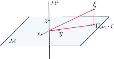
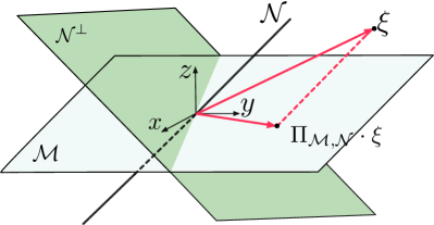
Figure 3: (a) Illustration of the orthogonal projection of a vector $\xi\in{}^{3}$ onto $\mathcal{M}\subset{}^{3}$. (b) Illustration of complementary subspaces $\mathcal{M},\mathcal{N}\in{}^{3}$ and oblique projection of $\xi$. Notice that the projection ray belongs to $\operatorname{span}(\mathcal{N})$.

Remark 4.6.

(Geometric interpretation of agreement space of consensus algorithms) In the case of consensus, the group of agents is known to converge to $\mathds{1}w^{\mathsf{T}}x(0)$, where $w$ is the left eigenvector of $A$ that satisfies $w^{\mathsf{T}}\mathds{1}=1$ (see Remark 3.2). By noting that $\mathds{1}w^{\mathsf{T}}x(0)=\Pi_{\mathcal{M},\mathcal{N}}x(0)$ is the oblique projection of $x(0)$ onto $\mathcal{M}=\operatorname{Im}(\mathds{1})$ along $\mathcal{N}=\operatorname{Im}(w)^{\bot}$ (see Lemma 2.2), Proposition 4.4 provides a geometric characterization of the agreement space. In the case of average consensus, the value at convergence is $\frac{1}{n}\mathds{1}\mathds{1}^{\mathsf{T}}x(0)$, which is the orthogonal projection of $x(0)$ onto $\mathcal{M}=\operatorname{Im}(\mathds{1})$.  $\square$

Motivated by the conclusions in Proposition 4.4, in what follows we make the following assumption.

Assumption 1

(Matrix of weights is a projection) The matrix of weights $W$ is a projection. Namely, $W\in{}^{n\times n},$ $W^{2}=W,$ and $\operatorname{rank}\left(W\right)=k$. $\square$

Notice that, given two complementary subspaces $\mathcal{M},\mathcal{N},$ a matrix $W$ that satisfies Assumption 1 can be computed as:

$$W=M(N^{\mathsf{T}}M)^{\scalebox{0.75}[0.9]{$-$}1}N^{\mathsf{T}},$$

where $M\in{}^{n\times k}$ and $N\in{}^{n\times k}$ form a basis for $\mathcal{M}$ and $\mathcal{N}^{\bot}$, respectively (see Lemma 2.2). Notice that the agreement space corresponding to this choice of $W$ is $\Pi_{\mathcal{M},\mathcal{N}}$.

With this background, we are now ready to provide a preliminary answer to Problem 1: in the the following result, we give a sufficient condition in terms of $\mathcal{G}$ that guarantees globally agreement reachability on arbitrary weights.

Proposition 4.7.

(Existence of agreement algorithms over complete digraphs) Let $\mathcal{M},\mathcal{N}\subset{}^{n}$ be complementary subspaces and $\mathcal{G}$ the complete graph with $|\mathcal{V}|=n$. Then, there exists $A\in{}^{n\times n}$, consistent with $\mathcal{G},$ such that the iterates (2) satisfy $\lim_{t\rightarrow\infty}x(t)=\Pi_{\mathcal{M},\mathcal{N}}x(0)$. $\square$

Proof 4.8.

For any pair of complementary subspaces $\mathcal{M},\mathcal{N},$ [32, Thm. 2.26] guarantees the existence of an oblique projection matrix $\Pi_{\mathcal{M},\mathcal{N}}$. Moreover, by Lemma 2.1, there exists invertible $T_{\Pi}\in{}^{n\times n}$ such that $\Pi_{\mathcal{M},\mathcal{N}}$ can be decomposed as

$$\Pi_{\mathcal{M},\mathcal{N}}=T_{\Pi}\begin{bmatrix}I_{k}&\mymathbb{0}\\ \mymathbb{0}&\mymathbb{0}\end{bmatrix}T_{\Pi}^{\scalebox{0.75}[0.9]{$-$}1},$$

where $k=\dim(\mathcal{M})$. The statement follows by choosing $A$ as in (5) with $T=T_{\Pi}$ and by noting that, with this choice, $\lim_{t\rightarrow\infty}e^{At}x(0)=\Pi_{\mathcal{M},\mathcal{N}}x(0)$.

Proposition 4.7 provides a preliminary answer to Problem 1 by showing that, if the communication graph is complete, the set of agents is globally $k$-agreement reachable on arbitrary weights. In the subsequent sections (sections 5 and 6), we will refine this result by seeking graphs with weaker connectivity that guarantee agreement reachability. The proof of the proposition provides a constructive way to derive protocols $A$ from $\mathcal{M}$ and $\mathcal{N}$. We formalize such a procedure in Algorithm 1. We remark that for some special choices of $\mathcal{M},\mathcal{N},$ one or more entries of $A$ may be identically zero (notice that such $A$ remain consistent with complete graphs, see Section 2); however, in the general case, $A$ is nonsparse.

Algorithm 1 Construction of agreement matrix $A$

0:  $M\in{}^{n\times k}$ whose columns form a basis for $\mathcal{M}$

0:  $N\in{}^{n\times k}$ whose columns form a basis for $\mathcal{N}^{\bot}$

  $\Pi_{\mathcal{M},\mathcal{N}}\leftarrow M(N^{\mathsf{T}}M)^{\scalebox{0.75}[0.9]{$-$}1}N^{\mathsf{T}}$;

  Determine $T$ such that $\Pi_{\mathcal{M},\mathcal{N}}=T\begin{bmatrix}I_{k}&\mymathbb{0}\\ \mymathbb{0}&\mymathbb{0}\end{bmatrix}T^{\scalebox{0.75}[0.9]{$-$}1}$;

  Choose $B\in{}^{(n-k)\times(n-k)}$ such that ${\lambda}_{\textup{max}}\left(B\right)<0$;

  return  $A=T\begin{bmatrix}\mymathbb{0}_{k}&\mymathbb{0}\\ \mymathbb{0}&B\end{bmatrix}T^{\scalebox{0.75}[0.9]{$-$}1}$;

4.2 Structural necessary conditions for agreement

While Proposition 4.7 shows that complete graphs guarantee global agreement reachability on arbitrary weights, it is natural to ask whether graphs with weaker connectivity are globally agreement reachable. Since the agreement problem generalizes that of consensus, to address this question, we next recall some known properties of consensus algorithms.

Remark 4.9.

(The role of connectivity in consensus) For consensus problems, [33] shows that a group of agents is globally consensus reachable if and only if the communication digraph contains a spanning tree. Intuitively, a spanning tree allows information to flow from the root node toward the rest of the graph; notice that, if the communication digraph is precisely a spanning tree, the value at consensus must coincide with the initial state of the root node, as there is no way for the root to receive information from the others. On the other hand, [34] shows that a group of agents is globally average consensus reachable if and only if the communication graph is strongly connected. Intuitively, in a strongly connected network, the initial state of each node can propagate to any other node.  $\square$

Despite strong connectivity being necessary and sufficient for average consensus reachability, the following counter-example shows that it is no longer sufficient for agreement reachability on arbitrary weights.

Example 4.10.

(Strong connectivity alone is not sufficient for agreement reachability on arbitrary weights) Assume that a network of $n=3$ agents is interested in agreeing on a space with $k=2$ by using a non-complete communication graph $\mathcal{G}$. By using Lemma 4.1, when the set of agents is agreement reachable on arbitrary weights, the following condition holds:

$$A=\underbrace{\begin{bmatrix}t_{1}&t_{2}&t_{3}\end{bmatrix}}_{=T}\begin{bmatrix}0&0&0\\ 0&0&0\\ 0&0&\beta\end{bmatrix}\underbrace{\begin{bmatrix}\tau_{1}&\tau_{2}&\tau_{3}\end{bmatrix}^{\mathsf{T}}}_{=T^{\scalebox{0.75}[0.9]{$-$}1}}=\beta t_{3}\tau_{3}^{\mathsf{T}},$$ (7)

for some $\beta$ such that $\Re(\beta)<0$ and some $T\in{}^{3\times 3}$ invertible. Since $\mathcal{G}$ is non-complete by assumption, at least one of the entries of $A$ must be identically zero, and thus, since $A$ is a rank-$1$ matrix by (7), at least one of its rows or columns must be identically zero; this implies that $\mathcal{G}$ cannot be strongly connected. By application of [36, Cor 4.5], we find that at least one of the rows or columns of $W=\lim_{t\rightarrow\infty}e^{At}$ must be identically zero. In summary, we have found that the agents are globally $2$-agreement reachable on arbitrary weights only if $\mathcal{G}$ is the complete graph. Notice, however, that the set of agents can be globally agreement reachable on some weights (precisely, $W$ must have an identically zero row or column).  $\square$

The above discussion highlights a fundamental difference between consensus and agreement protocols: agreement algorithms require communication digraphs with higher connectivity as compared to consensus algorithms. Intuitively, this is not surprising as agreement protocols seek to compute multiple independent quantities using the same communication volume (cf. Fig. 1). The following remark shows that strong connectivity remains a necessary assumption for agreement.

Remark 4.11.

(Necessity of strong connectivity) When $\mathcal{G}$ is not strongly connected, then for any $A$ that is consistent with $\mathcal{G}$ at least one of the entries of the matrix exponential $W=\lim_{t\rightarrow\infty}e^{At}$ is identically zero (this follows by recalling that $e^{At}=\sum_{i=0}^{\infty}\frac{A^{i}t^{i}}{i!}$ and from [36, Cor 4.5]). Thus, when $\mathcal{G}$ is not strongly connected, the set of agents is not globally agreement reachable on arbitrary weights. $\square$

Motivated by the above findings, in the remainder of this paper we make the following necessary assumption.

Assumption 2

(Strong connectivity) The communication digraph $\mathcal{G}$ is strongly connected. $\square$

5 Agreement algorithms over sparse digraphs

In the previous section, we found that complete connectivity is a sufficient condition for agreement reachability on arbitrary weights but, on the other hand, strong connectivity is not. Hence, the class of communication graphs that are agreement reachable on arbitrary weights must lay between these two classes. In this section, we derive algebraic conditions to determine this class of graphs (and thus to address Problem 1). In the second part of this section, we use this characterization to provide a solution to Problem 2.

In what follows, we will often use the following decomposition for $W$ (see Assumption 1 and Lemma 2.1):

$$W =T_{W}\begin{bmatrix}I_{k}&\mymathbb{0}\\ \mymathbb{0}&\mymathbb{0}\end{bmatrix}T_{W}^{\scalebox{0.75}[0.9]{$-$}1},$$ (8)

where $T_{W}\in{}^{n\times n}$ is invertible. Moreover, we will use:

$$T_{W} =\begin{bmatrix}t_{1}&\cdots&t_{n}\end{bmatrix}, T_{W}^{\scalebox{0.75}[0.9]{$-$}1} =\begin{bmatrix}\tau_{1}&\cdots&\tau_{n}\end{bmatrix}^{\mathsf{T}},$$ (9)

where $t_{i},\tau_{i}\in{}^{n},$ $i\in\{1,\dots,n\}$ (notice that $\tau_{i}^{\mathsf{T}}t_{j}=1$ if $i=j$ and $\tau_{i}^{\mathsf{T}}t_{j}=0$ otherwise).

5.1 Algebraic conditions for agreement

As noted in Remark 3.5, the Perron-Frobenius theory can no longer be applied to design agreement protocols, and thus we have to resort on new tools to provide a complete answer to Problem 1. To this aim, in this paper, we leverage the structural approach to system theory [30, 31] to derive an algebraic characterization for agreement protocols. Our characterization builds upon a graph-theoretic interpretation of characteristic polynomials [40], which we recall next. Let $\mathcal{C}_{\ell}(\mathcal{G})$ denote the set of all Hamiltonian $\ell$-decomposition of the graph $\mathcal{G}$ (see Section 2).

Lemma 5.1.

( ​​[40, Thm. 1]) Let $\mathcal{G}$ be a digraph, let $A\in\mathcal{A}_{\mathcal{G}}$, and $\det(\lambda I-A)=\lambda^{n}+p_{1}\lambda^{n-1}+\dots+p_{n-1}\lambda+p_{n}$ denote its characteristic polynomial. Each coefficient $p_{\ell},\ell\in\{1,\dots,n\},$ can be written as:

$$p_{\ell}=\sum_{\xi\in\mathcal{C}_{\ell}(\mathcal{G})}(\scalebox{0.75}[0.9]{$-$}1)^{d(\xi)}\prod_{(i,j)\in\xi}a_{ij},$$

where $d(\xi)$ denotes the number of Hamiltonian cycles in $\xi$. $\square$

The lemma provides a graph-theoretic description of the characteristic polynomial: it shows that the $\ell$-th coefficient of $\det(\lambda I-A)$ is a sum of terms such that each summand is the product of edges in a Hamiltonian $\ell$-decomposition of $\mathcal{G}$. We illustrate the claim through an example.

Example 5.2.

Consider the digraph in Figure 2(a). We have:

$$A=\begin{bmatrix}a_{11}&0&a_{13}&0\\ a_{21}&0&a_{23}&0\\ 0&a_{32}&0&a_{34}\\ 0&a_{42}&0&0\\ \end{bmatrix},$$

and we refer to Figure 2(b)-(c) for an illustration of all Hamiltonian $\ell$-decompositions for this graph. Lemma 5.1 yields:

$$p_{1} =-a_{11}, p_{3} =-a_{13}a_{21}a_{32}+a_{11}a_{23}a_{32}-a_{23}a_{42}a_{34},$$

$$p_{2} =-a_{23}a_{32} p_{4} =-a_{13}a_{21}a_{42}a_{34}+a_{11}a_{23}a_{34}a_{42}.$$

Notice that each summand in $p_{\ell}$ is the product of weights in a Hamiltonian decomposition of the corresponding size. $\square$

The following result is one of the main contributions of this paper, and provides a necessary and sufficient condition for a matrix $A$ to be an agreement protocol. Recall that we use the notation $\mathbf{A}_{\mathcal{G}}(a)$ to denote matrices $A$ in (2) that are consistent with $\mathcal{G}$ and whose entries are parametrized by $a\in{}^{|\mathcal{E}|}$ (see Section 2).

Theorem 5.3.

(Algebraic characterization of sparse agreement matrices) Let Assumptions 1-2 hold. The linear update $\dot{x}=\mathbf{A}_{\mathcal{G}}(a)x$ reaches a $k$-dimensional agreement on $W$ if and only if the following conditions hold simultaneously:

• $\mathbf{A}_{\mathcal{G}}(a)t_{i}=0,\quad\tau_{i}^{\mathsf{T}}\mathbf{A}_{\mathcal{G}}(a)=0,\quad\quad\forall i\in\{1,\dots,k\}$;

• The polynomial $\lambda^{n-k-1}+p_{1}\lambda^{n-k-2}+\dots+p_{n-k-1}$, whose coefficients are defined as

  $$p_{\ell} =\sum_{\xi\in\mathcal{C}_{\ell}(\mathcal{G})}(\scalebox{0.75}[0.9]{$-$}1)^{d(\xi)}\prod_{(i,j)\in\xi}a_{ij}, \ell\in\{1,\dots,n-k\},$$

  is stable. $\square$

Proof 5.4.

(If) Let $A$ be any matrix that satisfies (i)-(ii). If $A$ is diagonalizable, then, by letting $T=(t_{1},\cdots,t_{n})$ be the matrix of its right eigenvectors and $(T^{\scalebox{0.75}[0.9]{$-$}1})^{\mathsf{T}}=(\tau_{1},\cdots,\tau_{n})$ be the matrix of its left eigenvectors, we conclude that $A$ satisfies (5) and thus the linear update reaches an agreement on $W$. If $A$ is not diagonalizable, let $T$ be a similarity transformation such that $T^{\scalebox{0.75}[0.9]{$-$}1}AT$ is in Jordan normal form:

$$T^{\scalebox{0.75}[0.9]{$-$}1}AT=\begin{bmatrix}J_{\lambda_{1}}\\ &J_{\lambda_{2}}\\ &&\ddots\\ &&&J_{\lambda_{n}}\end{bmatrix},J_{\lambda_{i}}=\begin{bmatrix}\lambda_{1}&1\\ &\ddots&\ddots\\ &&\lambda_{1}\\ \end{bmatrix},$$

From (i) we conclude that $\lambda=0$ is an eigenvalue with algebraic multiplicity $k$, moreover, since the vectors $t_{i}$ are linearly independent (see (8)), we conclude that its geometric multiplicity is also equal to $k$, and thus all Jordan blocks associated with $\lambda=0$ have dimension $1$. Namely, $J_{\lambda_{1}}=\dots=J_{\lambda_{k}}=0$. By combining this with (ii), we conclude that the characteristic polynomial of $A$ is

$$\det(\lambda I-A) =\lambda^{n}+p_{1}\lambda^{n-1}+\dots+p_{n-k-1}\lambda^{k-1},$$

and, since by assumption such polynomial is stable, we conclude that all remaining eigenvalues $\{\lambda_{k+1},\dots,\lambda_{n}\}$ of $A$ satisfy $\Re(\lambda_{i})<0$. Since all Jordan blocks associated with $\lambda=0$ have dimension $1$ and all the remaining eigenvalues of $A$ are stable, we conclude that $A$ admits the representation (5) and thus the linear update reaches an agreement.

(Only if) We will prove this claim by showing that (5) implies (i)-(ii). To prove that (i) holds, we rewrite (5) as

$$T^{\scalebox{0.75}[0.9]{$-$}1}AT=\begin{bmatrix}\mymathbb{0}&\mymathbb{0}\\ \mymathbb{0}&B\end{bmatrix},$$

and, by taking the first $k$ columns of the above identity we conclude $At_{i}=0$, $i\in\{1,\dots,k\}$, thus showing that (i) holds. To prove that (ii) holds, notice that (5) implies that the characteristic polynomial of $A$ is a stable polynomial with $k$ roots at zero. Namely,

$$\det(\lambda I-A) =\lambda^{k}(\lambda-\lambda_{1})(\lambda-\lambda_{2})\cdots(\lambda-\lambda_{n-k})$$

$$=\lambda^{n}+p_{1}\lambda^{n-1}+\dots+p_{n-k-1}\lambda^{k-1},$$

where $\Re(\lambda_{i})<0,i\in\{1,\dots,n-k\},$ and $p_{j},j\in\{1,\dots,n-k-1\},$ are nonzero real coefficients. The statement (ii) thus follows by applying the graph-theoretic interpretation of the coefficients of the characteristic polynomial in Lemma 5.1.

Theorem 5.3 provides an algebraic characterization of linear agreement protocols. Given a graph $\mathcal{G}$ and a matrix of weights $W$, the result can be used to construct agreement protocols as follows: interpreting the vector of edge parameters $a$ as well as $p_{1},\dots p_{n-k}$ as an unknowns, (i)-(ii) define a system of $2nk$ linear equations and $n-k$ multilinear polynomial equations with $|\mathcal{E}|+n-k$ unknowns. We remark that the solvability of these equations is not guaranteed in general (except in some special cases, such as when the digraph is complete, see Proposition 4.7) and that existence of solutions depends upon the connectivity of the underlying graph. In general cases, solvability can be assessed via standard techniques to solve systems of polynomial equations. We discuss one of these techniques in the following remark.

Remark 5.5.

(Determining solutions to systems of polynomial equations) A powerful technique for determining solutions to systems of polynomial equations uses the tool of Gröbner bases, as applied using Buchberger’s algorithm [42]. The technique relies on transforming the system of equations into a canonical form, expressed in terms of a Gröbner basis, for which it then easier to determine a solution. We refer to [42, 43] for a complete discussion. Furthermore, existence of solutions can be assessed using Hilbert’s Nullstellensatz theorem [43]. In short, the theorem guarantees that a system of polynomial equations has no solution if and only if its Gröbner basis is $\{1\}$. In this sense, the Gröbner basis method provides an easy way to check solvability of (i)-(ii). We also note that the computational complexity of solving systems of polynomial equations via Gröbner bases is exponential [43].  $\square$

5.2 Fast distributed agreement algorithms

In this section, we use the characterization of Theorem 5.3 to provide an answer to Problem 2. The freedom in the choice of the polynomial coefficients $p_{1},\dots p_{n-k}$ suggests that a certain graph may admit an infinite number of compatible agreement protocols. For this reason, we will now leverage such freedom to determine agreement protocols with optimal rate of convergence. Problem 2 can be made formal as follows:

$$\underset{A}{\text{min}}~{}~{}~{} r(A)$$

s.t. $$A\in\mathcal{A}_{\mathcal{G}},\quad\lim_{t\rightarrow\infty}e^{At}=W.$$ (10)

In (5.2), $r:{}^{n\times n}\rightarrow\real$ is a function that measures the rate of convergence of $e^{At}$. Notice that the optimization problem (5.2) is feasible if and only if there exists matrices $A$, compatible with $\mathcal{G},$ that are semi-convergent [36]. The problem of determining the fastest distributed agreement algorithm (5.2) is closely related to the problem of fastest average consensus studied in [20]; the main difference is that while the average consensus problem is always feasible when $\mathcal{G}$ is strongly connected, there is no simple way to check the feasibility of (5.2) in general (see Section 4.2).

When the optimization problem (5.2) is feasible, it is natural to consider two possible choices for the cost function $r(\cdot)$, motivated by the size of $\|e^{At}\|$ as a function of time. The first limiting case is $t\rightarrow\infty$. In this case, we consider the following asymptotic measure of convergence motivated by [44, Ch. 14]:

$$r_{\infty}(A):=\lim_{t\rightarrow\infty}t^{\scalebox{0.75}[0.9]{$-$}1}\log\|e^{At}\|={\lambda}_{\textup{max}}\left(A\right).$$ (11)

Recall that ${\lambda}_{\textup{max}}\left(A\right)$ denotes the spectral abscissa of $A$ (see Section 2). The second limiting case is $t\rightarrow 0$. In this case, we consider the following measure of the initial growth rate:

$$r_{0}(A):=\frac{d}{dt}\|e^{At}\|\bigg{|}_{t=0} =\lim_{t\downarrow 0}t^{\scalebox{0.75}[0.9]{$-$}1}\log\|e^{At}\|$$

$$={\lambda}_{\textup{max}}\left(\frac{A+A^{\mathsf{T}}}{2}\right),$$ (12)

where ${\lambda}_{\textup{max}}\left(\frac{A+A^{\mathsf{T}}}{2}\right)$ is the numerical abscissa of $A$ [44]. Accordingly, we have the following two results.

Proposition 5.6.

(Fast agreement via spectral abscissa minimization) Let Assumptions 1-2 hold. Assume that the optimization problem (5.2) is feasible, and let the performance measure be $r(\cdot)=r_{\infty}(\cdot)$. Any solution to the following optimization problem:

$$\min_{a\in{}^{|\mathcal{E}|}}~{}~{} {\lambda}_{\textup{max}}\left(\mathbf{A}_{\mathcal{G}}(a)\right)$$ (13)

s.t. $$\mathbf{A}_{\mathcal{G}}(a)t_{i}=0,~{}~{}\tau_{i}^{\mathsf{T}}\mathbf{A}_{\mathcal{G}}(a)=0,\quad\quad i\in\{1,\dots,k\},$$

where $t_{i},\tau_{i}$ are as in (9), is also a solution of (5.2). $\square$

Proof 5.7.

Since the optimization problem (5.2) is feasible, condition (i) of Theorem 5.3 guarantees that (13) is also feasible and that ${\lambda}_{\textup{max}}\left(\mathbf{A}_{\mathcal{G}}(a)\right)<0$. Let $a^{*}$ denote a solution of (13), and let $A=\mathbf{A}_{\mathcal{G}}(a^{*})$. By construction, we have $A\in\mathcal{A}_{\mathcal{G}}$, while the two constraints in (13), together with ${\lambda}_{\textup{max}}\left(A\right)<0$ (which is guaranteed by feasibility), guarantee that $\lim_{t\rightarrow\infty}e^{At}=W$, which shows that $a^{*}$ is a feasible point for (5.2). The claim thus follows by noting that the cost functions of (5.2) and that of (13) coincide.

Proposition 5.6 allows us to recast (5.2) as a finite-dimensional search over the parameters $a\in{}^{|\mathcal{E}|}$. Unfortunately, even though the constraints of (13) are linear equalities, finding a solution may be computationally burdensome because the objective function is not convex (in fact, it is not even Lipschitz [45]). On the other hand, we have the following.

Proposition 5.8.

(Fast agreement via numerical abscissa minimization) Let Assumptions 1-2 hold. Assume that the optimization problem (5.2) is feasible, and let the performance measure be $r(\cdot)=r_{0}(\cdot)$. Any solution to the following convex optimization problem:

$$\min_{a\in{}^{|\mathcal{E}|}}~{}~{} {\lambda}_{\textup{max}}\left(\frac{\mathbf{A}_{\mathcal{G}}(a)+\mathbf{A}_{\mathcal{G}}(a)^{\mathsf{T}}}{2}\right)$$ (14)

s.t. $$\mathbf{A}_{\mathcal{G}}(a)t_{i}=0,~{}~{}\tau_{i}^{\mathsf{T}}\mathbf{A}_{\mathcal{G}}(a)=0,\quad\quad i\in\{1,\dots,k\},$$

where $t_{i},\tau_{i}$ are as in (9), is also a solution of (5.2). $\square$

Proof 5.9.

The proof repeats the same steps as those in the proof of Proposition 5.6, by replacing the cost with (5.2).

In contrast with the spectral abscissa formulation (13), the cost function in (14) is always convex in the parameter $a$, and thus a global solution of (14) can be computed efficiently.

6 Graph-theoretic conditions for agreement

In this section, we use the characterization of Theorem 5.3 to provide a graph-theoretic answer to Problem 1. In fact, although Theorem 5.3 provides an explicit way to construct agreement protocols, the system of equations to be solved may not admit a solution (see, e.g., Example 4.10). Motivated by this observation, in this section we seek structural conditions on $\mathcal{G}$ that guarantee the solvability of such equations. We begin with a necessary condition.

Proposition 6.1.

(Graph-theoretic necessary conditions) Let Assumptions 1-2 hold. The set of agents is globally $k$-agreement reachable on arbitrary weights only if

$$|\mathcal{E}|\geq kn.$$ (15)

$\square$

Proof 6.2.

It follows from the algebraic characterization in Theorem 5.3 that $\dot{x}=\mathbf{A}_{\mathcal{G}}(a)x$ reaches an agreement if and only if the following set of algebraic equations admit a solution $a$:

$$0 =\mathbf{A}_{\mathcal{G}}(a)t_{i}, i\in\{1,\dots,k\},$$ (16a)

$$p_{\ell} =\sum_{\xi\in\mathcal{C}_{\ell}(\mathcal{G})}(\scalebox{0.75}[0.9]{$-$}1)^{d(c)}\prod_{(i,j)\in\xi}a_{ij}, \ell\in\{1,\dots,n-k\}.$$ (16b)

The system of equations (16) to be solved consists of $nk$ linearly independent linear equations and $n-k$ nonlinear equations with $|\mathcal{E}|$ unknowns and $n-k$ arbitrarily chosen real numbers $p_{1},\dots,p_{n-k}$. Due to the invertibility of matrix $T$, the equations (16a) are linearly independent and thus generic solvability of (16) requires the following necessary condition $|a|=|\mathcal{E}|\geq nk$.

Condition (15) can be interpreted as a lower bound on the minimal graph connectivity that is required to achieve agreement: the number of edges in $\mathcal{G}$ must grow at least linearly with $k$ or with $n$. The following remark discusses the above bound in the special case $k=1$.

Remark 6.3.

(Strong connectivity implies (15) when $k=1$) It is natural to ask whether condition (15) holds for established consensus algorithms on common digraphs (recall that in this case $k=1$). Consider the one-directional circular digraph (see Fig. 4(a)): this graph has $|\mathcal{E}|=2n,$ and thus (15) reads as $2n\geq 1\cdot n,$ which holds true for any $n.$ Notice that this digraph is the graph with minimal edge-set cardinality that is strongly connected and thus offers the tightest bound in (15). Similarly, for the bi-directional circular digraph (see Fig. 4(b)) and the bi-directional line digraph (see Fig. 4(d)), we have $|\mathcal{E}|=3n$ and $|\mathcal{E}|=3(n-2)+4,$ respectively. Hence, (15) is always satisfied for consensus protocols. $\square$

The condition (15) has some important implications on two widely-studied topologies: line and circulant digraphs. We discuss these cases in the following remarks.

Remark 6.4.

(Agreement over circulant digraphs) Consider the one-directional circulant topology in Fig. 4(a). In this case, $|\mathcal{E}|=2n$ and thus (15) yields the necessary condition $k\leq 2$. Similarly, consider the (bi-directional) circulant topology in Fig. 4(b). Here, $|\mathcal{E}|=3n$, and thus (15) yields the necessary condition $k\leq 3$. In words, the one-directional and bi-directional circulant digraphs allow agreement on subspaces of dimension at most $2$ and $3$, respectively.

Given an arbitrary $k\in\mathbb{N}_{>0}$ and a circulant-type communication digraph where each agent communicates with $\alpha\in\mathbb{N}_{>0}$ neighbors (see Fig. 4(c)), it is natural to ask: what is the smallest $\alpha$ that is needed to guarantee $k$-agreement reachability on arbitrary weights? By using (15) with $|\mathcal{E}|=n(\alpha+1)$, an answer to this question is the necessary condition: $\alpha\geq k-1,$ which illustrates that the communication degree $\alpha$ must grow at least linearly with $k$.  $\square$

Remark 6.5.

(Agreement over line digraphs) Consider the directed digraph with bi-directional line topology illustrated in Fig. 4(d). In this case, $|\mathcal{E}|=n+2(n-1)$, and thus (19) yields $k\leq\left\lfloor\frac{3n-2}{n}\right\rfloor,$ which implies $k\leq 3$. Thus, similarly to the circulant digraphs, bi-directional line topologies allow agreement on subspaces of dimension at most $3$.

Given an arbitrary $k\in\mathbb{N}_{>0}$ and a line-type communication digraph where each agent communicates with $\alpha\in\mathbb{N}_{>0}$ neighbors (see Fig. 4(e)), it is natural to ask: what is the smallest $\alpha$ that is needed to guarantee $k$-agreement reachability on arbitrary weights? By using (15) with $|\mathcal{E}|=n+\alpha n-\frac{\alpha}{2}(\frac{\alpha}{2}+1)$, simple computations yield the necessary condition: $\alpha\geq 2k-1$. Not surprisingly, this condition is more stringent than the circulant topology case (cf. Remark 6.4) since the cardinality of the edge-set of the line topology is smaller than that of the circulant topology (due to the lack of symmetry in the head and tail nodes – see Fig. 4(e)). $\square$

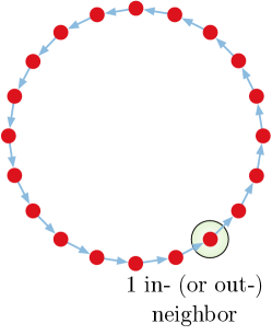
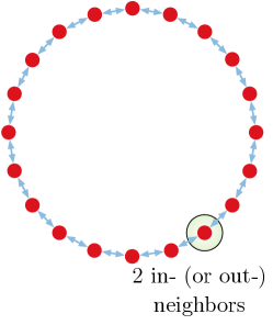
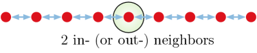
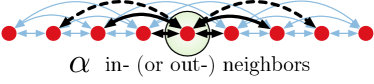
Figure 4: (a) One-directional circulant topology; (b)–(c) bi-directional circulant topology; (d)-(e) bi-directional line topology. The graph in (a) is the least-connected graph that can reach an agreement on $k=1$ (see Remark 6.3). (a), (b), and (d) can reach an agreement on subspaces of dimension at most $k=1$ (see Remarks 6.4, 6.5). In (c) and (d), to reach agreement on arbitrary $k$, $\alpha$ must grow at least linearly with $k$ (see Remarks 6.4, 6.5). In all plots, all nodes have self-cycles, which are omitted here for illustration purposes. Dashed lines illustrate the trend of edge increase as a function of $\alpha$.

The following result provides a graph-theoretic characterization of graphs that can achieve agreement on arbitrary weights.

Proposition 6.6.

(Graph-theoretic sufficient conditions) Let Assumptions 1-2 hold and let $|\mathcal{E}|\geq nk+n-k$. If there exists a partitioning of the edge parameters $a=(\{a_{ij}\}_{(i,j)\in\mathcal{E}})$ into two disjoint sets $a_{v}=\{a_{1},\dots a_{n-k}\}$ and $a_{c}=\{a_{n+1},\dots a_{|\mathcal{E}|}\}$ such that:

1. For all $\ell\in\{1,\dots,n-k\}$, there exists a Hamiltonian $\ell$-decomposition, denoted by $\mathcal{C}_{\ell}^{*}$, such that $a_{\ell}\in\mathcal{C}_{\ell}^{*}$;

2. Any edge in $\mathcal{C}_{\ell}^{*}$ other than $a_{\ell}$ belongs to $a_{c}$,

3. Any Hamiltonian $\ell$-decomposition other than $\mathcal{C}_{\ell}^{*}$ that contains edges in $a_{v}$ also contains at least one edge in $a_{c}$ that does not appear in $C_{\ell}^{*}$,

then the set of agents is globally $k$-agreement reachable on arbitrary weights. $\square$

Proof 6.7.

Recall from Thm. 5.3 that $\dot{x}=\mathbf{A}_{\mathcal{G}}(a)x$ reaches an agreement if and only if there exists a stable polynomial

$$P(\lambda)=\lambda^{n-k-1}+p_{1}\lambda^{n-k-2}+\dots+p_{n-k-1}.$$ (17)

with coefficients $p=(p_{1},\dots,p_{n-k})$ such that there exists a solution $a^{*}$ to the following set of algebraic equations:

$$0 =\mathbf{A}_{\mathcal{G}}(a)t_{i}, i\in\{1,\dots,k\},$$ (18a)

$$p_{\ell} =\sum_{\xi\in\mathcal{C}_{\ell}(\mathcal{G})}(\scalebox{0.75}[0.9]{$-$}1)^{d(c)}\prod_{(i,j)\in\xi}a_{ij}, \ell\in\{1,\dots,n-k\}.$$ (18b)

Hence, we prove this claim by showing that there exists a stable $P(\lambda)$ such that (18) admit a solution. Let $P(\lambda)$ be chosen as follows:

$$P(\lambda)=(\lambda-\alpha_{1})\cdots(\lambda-\alpha_{n}),$$

where its (either real or complex conjugate pairs) roots $\alpha_{i}\in\mathcal{\mathbb{C}},i\in\{1,\dots,n\}$, satisfy $\Re(\alpha_{i})<0$. Notice that $\Re(\alpha_{i})<0$ imply that all the coefficients $\{p_{1},\dots,p_{n-k}\}$ are non-negative. Since $\{\alpha_{1},\dots\alpha_{n}\}$ are arbitrary and for any such choice each element of $p=(p_{1},\dots,p_{n-k})$ is non-negative, we will seek solutions of (19) in a neighborhood of $p=0$.

Since $(t_{1},\dots t_{k})$ are given (and linearly independent), equation (18a) defines a set of $nk$ linearly independent equations in the variables $a=(a_{c},a_{v})$, which we denote compactly as $0=h(a_{c},a_{v})$, where $h:{}^{|\mathcal{E}|}\rightarrow{}^{nk}$. Equation (18b) relates $p$ and $(a_{c},a_{v})$ by meas of a nonlinear mapping $p=g(a_{c},a_{v})$, where $g:{}^{|\mathcal{E}|}\rightarrow\mathcal{T}$ is a smooth mapping and $\mathcal{T}$ is smooth manifold in ^n-k. Since $g(\cdot)$ is a multi-linear polynomial, it is immediate to verify that it admits the following decomposition:

$$g(a_{c},a_{v})=\frac{\partial g}{\partial a_{v}}\cdot a_{v}.$$

By denoting in compact form

$$G(a_{c},a_{v}) :=\frac{\partial g}{\partial a_{v}}\in{}^{n-k\times n-k},$$

$$H(a_{c},a_{v}) :=\frac{\partial h}{\partial a_{v}}\in{}^{nk\times n-k},$$

the system of equations (18) can be rewritten as

$$0 =H(a_{c},a_{v})a_{v},$$ (19a)

$$p =G(a_{c},a_{v})a_{v}.$$ (19b)

As discussed above, we will now seek solutions to (19) in a neighborhood of $p=0$. By the inverse function theorem [46, Thm. 9.24], solvability of (19) in a neighborhood of $p=0$ is guaranteed when there exists a particular point $(a_{c}^{*},a_{v}^{*})$ such that $0=H(a_{c}^{*},a_{v}^{*})a_{v}^{*}=G(a_{c}^{*},a_{v}^{*})a_{v}^{*}$ and $G(a_{c}^{*},a_{v}^{*})$ is invertible. To show this, we first notice that $a_{v}^{*}=0$ is a solution of (19) for any $a_{c}\in{}^{|\mathcal{E}|-n+k}$. Thus, we are left to show that there exists a choice $a_{c}^{*}$ such that $G(a_{c}^{*},a_{v}^{*})$ is invertible. Thus, we will next provide an inductive method to construct $a_{c}^{*}$ such that $G(a_{c}^{*},a_{v}^{*})$ is diagonally dominant.

Let $a_{c}^{(1)}\in{}^{|\mathcal{E}|-n+k}$ be an arbitrary choice for $a_{c}$ such that all its entries are nonzero. Notice that condition (i) in the statement guarantees that there exists a nonzero product in entry $(1,1)$ of $G(a_{c}^{(1)},a_{v}^{*})$, while condition (ii) guarantees that such product is independent of $a_{v}^{*}$. Thus, by letting $G^{(1)}(a_{c},a_{v}):=G(a_{c},a_{v})$, the matrix $G^{(1)}(a_{c}^{(1)},a_{v}^{*})$ can be partitioned as:

$$G^{(1)}(a_{c}^{(1)},a_{v}^{*})=\begin{bmatrix}G_{11}^{(1)}(a_{c}^{(1)})&G_{12}^{(1)}(a_{c}^{(1)},a_{v}^{*})\\[10.00002pt] G_{21}^{(1)}(a_{c}^{(1)},a_{v}^{*})&G_{22}^{(1)}(a_{c}^{(1)},a_{v}^{*})\end{bmatrix},$$

where $G_{11}^{(1)}\in\real$, $G_{12}^{(1)}\in{}^{1\times n-k-1}$, $G_{21}^{(1)}\in{}^{n-k-1\times 1}$, $G_{22}^{(1)}\in{}^{n-k-1\times n-k-1}$. By condition (ii) and since all entries of $a_{c}^{(1)}$ are nonzero, we have $G_{11}^{(1)}(a_{c}^{(1)})\neq 0$. Moreover, either no element of $a_{v}^{*}$ appears in any Hamiltonian $1$-decomposition, in which case we have $G_{12}^{(1)}(a_{c}^{(1)},a_{v}^{*})=0$ or, otherwise, by condition (iii), each entry in $G_{12}^{(1)}(a_{c}^{(1)},a_{v}^{*})$ is described by a product that contains at least one scalar variable in $a_{c}^{(1)}$ that does not appear in $G_{11}^{(1)}(a_{c}^{(1)})$. Denote such scalar variable by $\tilde{a}$ and notice that, by choosing $\tilde{a}$ sufficiently small, the first row of $G^{(1)}$ can be made diagonally dominant. Thus, we update $a_{c}^{(1)}$ as follows: $a_{c}^{(2)}=\min\{\tilde{a},a_{c}^{(i)}\}$ (where the minimum is taken entrywise).

For the inductive step $i$, notice that $G^{(i)}(a_{c}^{(i)},a_{v}^{*})$ is diagonally dominant if $G^{(i)}_{22}(a_{c}^{(i)},a_{v}^{*})$ is diagonally dominant. Thus, by defining $G^{(i+1)}(\cdot,\cdot)=G^{(i)}_{22}(\cdot,\cdot)$, $i\in\{1,\dots,n-1\}$, by letting $a_{c}^{(i+1)}=\min\{\tilde{a},a_{c}^{(i)}\}$ (entrywise minimum), and by iterating the argument, we conclude that $G(a_{c}^{(n-k)},a_{v}^{*})$ is diagonally dominant. Invertibility of $G(a_{c}^{*},a_{v}^{*})$ thus follows by letting $a_{c}^{*}=a_{c}^{(n-k)}$, which concludes the proof.

Proposition 6.6 gives a set of graph-theoretic sufficient conditions for agreement reachability on arbitrary weights. The result identifies Hamiltonian decompositions as the fundamental structural property that enables agreement reachability. Indeed, as shown in the proof, the existence of $n-k$ independent Hamiltonian decompositions in $\mathcal{G}$ guarantees that $a$ can be chosen so that $n-k$ modes of $\mathbf{A}(a)$ are stable. The usefulness of Proposition 6.6 depends largely on determining a partitioning of $a$ into two disjoint sets of variables $a_{v}$ and $a_{c}$. An algorithm to determine whether such partitioning exists can be constructed by using ideas similar to [47], where $a_{v}$ and $a_{c}$ are derived from a directed spanning tree of $\mathcal{G}$.

Remark 6.8.

(Minimal graphs for agreement) It is worth noting that if $\mathcal{G}=(\mathcal{V},\mathcal{E})$ admits the set of Hamiltonian $\ell$-decompositions $\mathcal{C}_{\ell}(\mathcal{G})$, then any graph $\mathcal{G}^{\prime}=(\mathcal{V}^{\prime},\mathcal{E}^{\prime})$ such that $\mathcal{V}^{\prime}=\mathcal{V}$ and $\mathcal{E}\subset\mathcal{E}^{\prime}$ has a set of Hamiltonian $\ell$-decompositions $\mathcal{C}_{\ell}^{\prime}(\mathcal{G})$ that satisfies $\mathcal{C}_{\ell}(\mathcal{G})\subseteq\mathcal{C}_{\ell}^{\prime}(\mathcal{G})$. It follows that if $\mathcal{G}$ is $k$-agreement reachable on arbitrary weights, then any digraph obtained by adding edges to $\mathcal{G}$ will also be $k$-agreement reachable on arbitrary weights $\square$

We conclude this section by demonstrating the applicability of Proposition. 6.6 through an example.

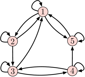
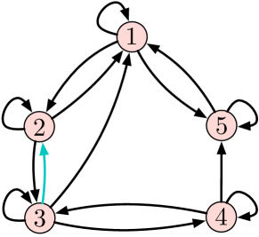
Figure 5: (a) Example of a graph that can sustain a $2$-dimensional agreement. (b) Graph obtained by adding green edges to (a); this graph can sustain a $3$-dimensional agreement. See Example 6.9.

Example 6.9.

(Illustration of Hamiltonian decomposition condition) Consider the communication graph illustrated in Fig. 5(a). The corresponding agreement protocol is given by:

$$\mathbf{A}_{\mathcal{G}}(a)=\begin{bmatrix}a_{11}&a_{12}&a_{13}&0&a_{15}\\ a_{21}&a_{22}&0&0&0\\ 0&a_{32}&a_{33}&a_{34}&0\\ 0&0&a_{43}&a_{44}&0\\ a_{51}&0&0&a_{54}&a_{55}\\ \end{bmatrix}.$$

By Proposition 6.1, a necessary condition for agreement is

$$k\leq\left\lfloor\frac{|\mathcal{E}|}{n}\right\rfloor=\left\lfloor\frac{14}{5}\right\rfloor=2,$$

Thus, in what follows we fix $k=2$. To illustrate the conditions of Proposition 6.6, for simplicity, we let $a_{22}=a_{33}=a_{44}=a_{55}=0$ (according to Remark 6.8, if the graph without self-cycles has an independent set of Hamiltonian decompositions, then the graph obtained by adding these self-cycles will retain the same set of decompositions). With this choice, the set of all Hamiltonian $\ell$-decompositions, $\ell\in\{1,\dots,n-k\}$, is:

$$\mathcal{C}_{1} =\{\{a_{11}\}\},$$

$$\mathcal{C}_{2} =\{\{a_{12},a_{21}\},\{a_{34},a_{43}\},\{a_{15},a_{51}\}\},$$

$$\mathcal{C}_{3} =\{\{a_{11},a_{34},a_{43}\},\{a_{13},a_{21},a_{32}\}\}.$$ (20)

By selecting $a_{v}$ and $a_{c}$ as follows

$$a_{v} =\{a_{11},a_{12},a_{13}\},$$

$$a_{c} =\{a_{51},a_{54},a_{21},a_{32},a_{34},a_{43},a_{15}\},$$

it follows that a set of Hamiltonian $\ell$-decompositions that satisfies the conditions in Proposition 6.6 is:

$$\mathcal{C}_{1}^{*} =\{a_{11}\}, \mathcal{C}_{2}^{*} =\{a_{12},a_{21}\}, \mathcal{C}_{3}^{*} =\{a_{13},a_{21},a_{32}\}.$$

Indeed, with this choice, the set of equations (16b) reads as:

$$\begin{bmatrix}p_{1}\\ p_{2}\\ p_{3}\end{bmatrix}=\begin{bmatrix}-1&0&0\\ 0&-a_{21}&0\\ a_{34}a_{43}&0&-a_{21}a_{32}\end{bmatrix}\begin{bmatrix}a_{11}\\ a_{12}\\ a_{13}\end{bmatrix}-\begin{bmatrix}0\\ \gamma\\ 0\end{bmatrix},$$

where $\gamma=a_{34}a_{43}+a_{15}a_{51}$, which is generically solvable for any $(p_{1},p_{2},p_{3})\in{}^{3}$. Any choice of weights such that $a_{21}>0$ and $|a_{21}a_{32}|>|a_{34}a_{43}|$ guarantees that the above matrix is invertible and thus the set of equations is solvable.

To achieve agreements on subspaces of dimension $k=3$, consider the graph in Fig. 5(b), obtained by adding edges to the graph of Fig. 5(a). The necessary condition (15) yields

$$k\leq\left\lfloor\frac{|\mathcal{E}|}{n}\right\rfloor=\left\lfloor\frac{15}{5}\right\rfloor=3,$$

which is satisfied. The set of relevant Hamiltonian decompositions (6.9) modifies to:

$$\mathcal{C}_{1} =\{\{a_{11}\}\},$$

$$\mathcal{C}_{2} =\{\{a_{12},a_{21}\},\{a_{34},a_{43}\},\{a_{15},a_{51}\},\{a_{23},a_{32}\}\}.$$

By selecting $a_{v}$ and $a_{c}$ as follows

$$a_{v} =\{a_{11},a_{12}\},$$

$$a_{c} =\{a_{13},a_{23},a_{45},a_{35},a_{51},a_{54},a_{21},a_{32},a_{34},a_{43},a_{15}\},$$

a set of Hamiltonian $\ell$-decompositions that satisfies Proposition 6.6 is:

$$\mathcal{C}_{1}^{*} =\{a_{11}\}, \mathcal{C}_{2}^{*} =\{a_{12},a_{21}\},$$

thus showing that the sufficient conditions also hold. $\square$

7 Tracking dynamics for agreement

In analogy with classical consensus processes [48], agreement protocols can be modified to track (the oblique projection of) a time-varying forcing signal $u(t)$. Specifically, given a graph $\mathcal{G}$, consider the network process

$$\dot{x} =\mathbf{A}_{\mathcal{G}}(a)x+\dot{u}, x(0) =u(0),$$ (21)

where $a$ is chosen so that $\mathbf{A}_{\mathcal{G}}(a)$ is an agreement matrix (as in Theorem 5.3) and $u:\mathbb{R}_{\geq 0}\rightarrow{}^{n}$ is a continuously-differentiable function. In this framework, the $i$-th entry of $\dot{u}$ is known only by agent $i$, and the objective is to guarantee that $x(t)$ tracks a $k$-dimensional projection $Wu(t)$ of $u(t)$ asymptotically. The protocol (21) can be interpreted as a generalization of the dynamic average consensus algorithm [48], where the communication matrix is an agreement matrix instead than a Laplacian. The following result characterizes the transient behavior of (21).

Proposition 7.1.

(Convergence of dynamic agreement protocol) Consider the update (21) and let $\mathbf{A}_{\mathcal{G}}(a)$ be an agreement protocol on $W$ as in Theorem 5.3. Then, for all $t\geq 0$:

$$\|x(t)-Wu(t)\|\leq e^{-\hat{\lambda}t}\|x(0)-Wu(0)\|+\frac{1}{\hat{\lambda}}\sup_{0\leq\tau\leq t}\|\dot{u}(\tau)\|,$$ (22)

where $\hat{\lambda}={\lambda}_{\textup{max}}\left(\frac{\mathbf{A}_{\mathcal{G}}(a)+\mathbf{A}_{\mathcal{G}}(a)^{\mathsf{T}}}{2}\right)$. $\square$

Proof 7.2.

The proof is inspired from [48, Thm. 2] and extends the result to non Laplacian-based protocols and non weight-balanced digraphs. Let $W$ be decomposed as in (8), and consider the following decompositions for $T_{W}$ and $T_{W}^{\scalebox{0.75}[0.9]{$-$}1}$:

$$T_{W} =\begin{bmatrix}T_{1}&T_{2}\end{bmatrix}, (T_{W}^{\scalebox{0.75}[0.9]{$-$}1})^{\mathsf{T}} =\begin{bmatrix}U_{1}&U_{2}\end{bmatrix},$$ (23)

where $T_{1},U_{1}\in{}^{n\times k}$ and $T_{2},U_{2}\in{}^{n\times n-k}$. Let $e=x-Wu$ denote the tracking error, and consider the change of variables $\bar{e}=T_{W}^{\scalebox{0.75}[0.9]{$-$}1}e$. In the new variables:

$$\dot{\bar{e}} =T_{W}^{\scalebox{0.75}[0.9]{$-$}1}(\dot{x}-W\dot{u})$$

$$=T_{W}^{\scalebox{0.75}[0.9]{$-$}1}AT_{W}\bar{e}+T_{W}^{\scalebox{0.75}[0.9]{$-$}1}AWu+T_{W}^{\scalebox{0.75}[0.9]{$-$}1}\dot{u}-T_{W}^{\scalebox{0.75}[0.9]{$-$}1}W\dot{u},$$

$$=T_{W}^{\scalebox{0.75}[0.9]{$-$}1}AT_{W}\bar{e}+T_{W}^{\scalebox{0.75}[0.9]{$-$}1}\dot{u}-T_{W}^{\scalebox{0.75}[0.9]{$-$}1}W\dot{u},$$

where the last identity follows by using (8), which implies $AW=0$. By substituting (23) and by noting that $T^{\scalebox{0.75}[0.9]{$-$}1}W=\left[U_{1}~{}0\right]^{\mathsf{T}}$:

$$\dot{\bar{e}} =\begin{bmatrix}U_{1}^{\mathsf{T}}AT_{1}&U_{1}^{\mathsf{T}}AT_{2}\\ U_{2}^{\mathsf{T}}AT_{1}&U_{2}^{\mathsf{T}}AT_{2}\end{bmatrix}\bar{e}+\begin{bmatrix}0\\ U_{2}^{\mathsf{T}}\end{bmatrix}\dot{u}$$

$$=\begin{bmatrix}0\\ U_{2}^{\mathsf{T}}AT_{2}\end{bmatrix}\bar{e}+\begin{bmatrix}0\\ U_{2}^{\mathsf{T}}\end{bmatrix}\dot{u},$$ (24)

where the last inequality follows by noting that $0=U_{1}^{\mathsf{T}}AT_{1}=U_{1}^{\mathsf{T}}=AT_{1}$ according to condition (i) in Theorem 5.3.

Next, decompose $e=(e_{1},e_{2})$ and $\bar{e}=(\bar{e}_{1},\bar{e}_{2})$, where $e_{1},\bar{e}_{1}\in{}^{k}$ and $e_{2},\bar{e}_{2}\in{}^{n-k}$, and notice that the following identities hold:

$$\bar{e}_{2} =U_{2}^{\mathsf{T}}e, e =T_{2}\bar{e}_{2}.$$ (25)

The first identity follows immediately from (23), while the second follows from (23) and $\bar{e}_{1}(t)=0$ at all times. To see that $\bar{e}_{1}(t)=0~{}\forall t\geq 0$, notice that $\bar{e}_{1}(0)=U_{1}^{\mathsf{T}}(x(0)-u(0))=0$ thanks to the initialization (21), and $\dot{\bar{e}}_{1}=0$ according to (7.2). By using (25), we conclude that $\dot{e}=Ae+\dot{u}$, from which (22) follows by noting that

$${e(t)}=\exp(At)\cdot e(0)+\int_{0}^{t}\exp(A(t-\tau))B\dot{u}(\tau)d\tau,$$

and by using $\|\exp(At)\|\leq\exp\left(-{\lambda}_{\textup{max}}\left(\frac{\mathbf{A}_{\mathcal{G}}(a)+\mathbf{A}_{\mathcal{G}}(a)^{\mathsf{T}}}{2}\right)t\right)$.

The error bound (22) shows that the dynamics (21) are input-to-state stable with respect to $\dot{u}$. The bound (22) guarantees that for any forcing signal $u(t)$ with bounded time-derivative the tracking error $\|x(t)-Wu(t)\|$ is bounded at all times. One important implication follows from the statement of the proposition as a subcase: if $\lim_{t\rightarrow\infty}u(t)=u^{*}\in{}^{n}$ (namely, $\lim_{t\rightarrow\infty}\dot{u}(t)=0$), then $\lim_{t\rightarrow\infty}x(t)=Wu^{*}$.

8 Applications and numerical validation

In this section, we expand on the examples discussed in Section 4.2 and illustrate the applicability of the methods via numerical simulations. We consider two application scenarios.

Sensor measurement de-noising. We consider a problem in distributed estimation characterized by a regression model of the form $y=H\theta$, where $H\in{}^{n\times k},n>k$ and $\theta\in{}^{k}$ is an unknown parameter. We assume that each agent $i$ can sense the $i$-th entry of vector $y$, denoted by $y_{i}$, and is interested in computing the point $\hat{y}_{i}$ that is the closest to $y_{i}$ according to the regression model. To this end, we consider the following regression problem:

$${\theta}_{\textup{ls}}:=\arg\min_{\theta}\|H\theta-y\|.$$ (26)

It is well-known that ${\theta}_{\textup{ls}}$ can be obtained as

$${\theta}_{\textup{ls}}=(H^{\mathsf{T}}H)^{\scalebox{0.75}[0.9]{$-$}1}H^{\mathsf{T}}y,$$

provided that $H^{\mathsf{T}}H$ is invertible (this is obtained by letting $0=\nabla_{\theta}\|H\theta-y\|^{2}=2H^{\mathsf{T}}H\theta-2H^{\mathsf{T}}y$). The desired vector to be computed by the agents (de-noised measurements) is

$$\hat{y}=H{\theta}_{\textup{ls}}=H(H^{\mathsf{T}}H)^{\scalebox{0.75}[0.9]{$-$}1}H^{\mathsf{T}}y,$$

which is the orthogonal projection of $y$ onto $\operatorname{Im}(H)$. For figure illustration purposes, we consider the case $n=50$ (meaning $n=50$ agents or sensors in the network) and $k=2$ (meaning the sensor measurements can be interpolated using a line). We computed an agreement protocol using the optimization problem (14) with weights $W=H(H^{\mathsf{T}}H)^{\scalebox{0.75}[0.9]{$-$}1}H^{\mathsf{T}}$ and implemented on the circulant graph of Fig. 4(c) with $\alpha=4$ in/out neighbors. Fig. 6(top) shows the sampling points $y$ and asymptotic estimates $\hat{y}$ in comparison with the true regression model. As expected, the distributed algorithm (1) converges to the data points corresponding to the Mean Square Error Estimator. Fig. 6(bottom) shows the trajectories of the agents states. As expected, at convergence, the states of the agents do not coincide, instead, the agreement state is a $50$-dimensional vector constrained to a $2$-dimensional subspace.

Robotic formation control. We next illustrate how agreement protocols can be applied to solve formation control problems [9] in multi-agent robotic networks. Consider a team of $n=8$ planar single-integrator robots initially arranged at equal intervals around a unit circle (grey lines in Fig. 7(a)-(c)). By using $x-$ and $y-$coordinates to describe the robots’ positions, we use $x_{0}=(\cos(0),\sin(0),\cos(\frac{\pi}{4}),\sin(\frac{\pi}{4}),\dots,\cos(\frac{7\pi}{4}),\sin(\frac{7\pi}{4}))\in{}^{16}$. Fig. 7 illustrates the trajectories of the robots obtained by using the 2D agreement protocol

$$\dot{x} =(A\otimes I_{2})x, x(0) =x_{0},$$

using the circulant communication graph illustrated in Fig. 7(b) with $\alpha=4$. For comparison, in Fig. 7(a) and (d) we illustrate the trajectories obtained by a consensus algorithm described by weights $W=\frac{1}{n}\mathds{1}\mathds{1}^{\mathsf{T}}$. As expected, the robots meet at the point $(0,0)$, thus achieving rendezvous [9]. In Fig.7(b) and (e), we illustrate the trajectories resulting from running an agreement protocol (computed by solving (14)) with weights $W=\Pi_{\mathcal{M}}$, where $\Pi_{\mathcal{M}}$ is the orthogonal projection onto $\mathcal{M}=\ker(M_{1})\subset{}^{8}$ with

$$M_{1}=\begin{bmatrix}1&-1&-1&1&0&0&0&0\\ 0&0&0&0&1&-1&-1&1\end{bmatrix}.$$

The matrix $M_{1}$ encodes attraction and repulsion forces between certain robots at convergence. Indeed, by recalling that the agreement value is $x(\infty)=\Pi_{\mathcal{M}}x(0)$, it follows that at steady state the agents’ positions satisfy $M_{1}x(\infty)=0$. Hence, the rows of $M_{1}$ are interpreted as algebraic constraints on the asymptotic agreement value. From Fig.7(b), which reports the corresponding time-evolution of the $x-$ and $y-$coordinates of the robots, we observe that the robots asymptotically achieve a formation that is characterized by a 2-dimensional subspace. Finally, Fig.s 7(d) and (f) illustrate the trajectories of the robots generated by an agreement protocol (computed by solving (13)) where the weights are described by an oblique projection $W=\Pi_{\mathcal{M},\mathcal{N}}$, where $\mathcal{M}=\ker(M_{1})\subset{}^{8}$ and $\mathcal{N}=\operatorname{Im}(N_{1})\subset{}^{8}$ with

$$N_{1}^{\mathsf{T}}=\begin{bmatrix}-1&5&5&-1&0&0&0&0\\ 0&0&0&0&-1&5&5&-1\end{bmatrix}.$$

The use of an oblique projection can be interpreted as a non-homogeneous weighting for the vector that defines the final configuration. Indeed, as shown by the figure, in this case, the robots no longer meet “halfway”, instead, robots $2$ and $3$ [respectively, $6$ and $7$] travel a longer distance as opposed to robots $1$ and $4$ [respectively, $5$ and $8$]).

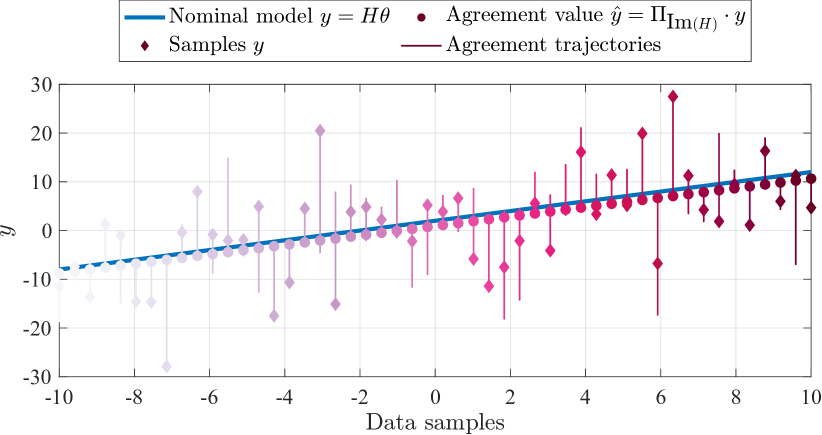
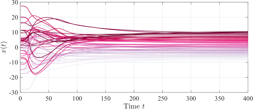
Figure 6: Application of agreement protocols to solve regression problems. Each agent can measure a sample $y_{i}$ (represented by diamond markers) and cooperatively computes the projection of $\hat{y}_{i}$ onto the range of the regression matrix $H$ (represented by circle markers), see (26). (Top figure) continuous lines illustrate the time evolution of the states of (1). (Bottom figure) Time evolution of the trajectories of (1). Notice that the agents’ states do not converge to the same value.

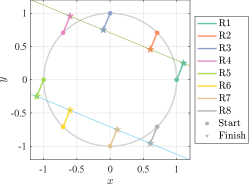
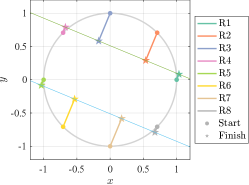
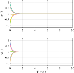
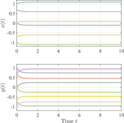
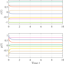
Figure 7: (a)-(c) Time evolution of the positions of the $8$ robots and (d)-(f) trajectories of the $x-$ and $y-$coordinates. (a) and (d) Consensus protocol, which allows the robots to achieve rendezvous. (b) and (e) Agreement protocol on an orthogonal projection onto $\ker(M_{1}).$ (c) and (f) Agreement on an oblique projection on $\ker(M_{1})$ along $\operatorname{Im}(N_{1})$.

9 Conclusions

We have studied the problem of $k$-dimensional agreement, whereby a group of agents would like to agree on a vector that is the projection of the agents’ initial estimates onto a $k$-dimensional subspace. We showed that agreement protocols mandate the use of communication graphs that are highly connected; to this end, we provided both algebraic and graph-theoretic conditions to construct graphs that can reach an agreement on arbitrary weights. The identified sufficient condition allows us to construct a class of graphs that can reach an agreement, but we conjecture that the class of agreement reachable graphs on arbitrary weights is much larger in practice. This work opens the opportunity for multiple directions of future research: among them, we highlight the derivation of algorithms that can define agreement protocols in a distributed way; the use of nonlinear dynamics as agreement protocols to enable convergence to agreement vectors that are not just oblique projections; and the synthesis of distributed and scalable coordination algorithms to solve optimization problems over networks, where the number of agents and the number of primal variables are of the same order.

References

- [1] V. D. Blondel, J. M. Hendrickx, A. Olshevsky, and J. N. Tsitsiklis, “Convergence in multiagent coordination, consensus, and flocking,” in IEEE Conf. on Decision and Control, 2005, pp. 2996–3000.
- [2] R. Olfati-Saber and R. M. Murray, “Consensus problems in networks of agents with switching topology and time-delays,” IEEE Transactions on Automatic Control, vol. 49, no. 9, pp. 1520–1533, 2004.
- [3] W. Ren, R. W. Beard, and E. M. Atkins, “A survey of consensus problems in multi-agent coordination,” in American Control Conference, Portland, OR, Jun. 2005, pp. 1859–1864.
- [4] G. Malewicz, M. H. Austern, A. J.-C. Bik, J. C. Dehnert, I. Horn, N. Leiser, and G. Czajkowski, “Pregel: a system for large-scale graph processing,” in International Conference on Management of data, 2010, pp. 135–146.
- [5] D. Peleg, Distributed Computing: a Locality-Sensitive Approach. SIAM, 2000.
- [6] H.-L. Choi, L. Brunet, and J. P. How, “Consensus-based decentralized auctions for robust task allocation,” IEEE Transactions on Robotics, vol. 25, no. 4, pp. 912–926, 2009.
- [7] L. Zhao and A. Abur, “Multi area state estimation using synchronized phasor measurements,” IEEE Transactions on Power Systems, vol. 20, no. 2, pp. 611–617, 2005.
- [8] F. Pasqualetti, R. Carli, A. Bicchi, and F. Bullo, “Distributed estimation and detection under local information,” in IFAC Workshop on Distributed Estimation and Control in Networked Systems, Annecy, France, Sep. 2010, pp. 263–268.
- [9] K.-K. Oh, M.-C. Park, and H.-S. Ahn, “A survey of multi-agent formation control,” Automatica, vol. 53, pp. 424–440, 2015.
- [10] J. N. Tsitsiklis, “Problems in decentralized decision making and computation,” Ph.D. dissertation, Massachusetts Institute of Technology, Nov. 1984, available at http://web.mit.edu/jnt/www/Papers/PhD-84-jnt.pdf.
- [11] A. Jadbabaie, J. Lin, and A. S. Morse, “Coordination of groups of mobile autonomous agents using nearest neighbor rules,” IEEE Transactions on Automatic Control, vol. 48, no. 6, pp. 988–1001, 2003.
- [12] M. Cao, A. S. Morse, and B. D. O. Anderson, “Reaching a consensus in a dynamically changing environment - convergence rates, measurement delays and asynchronous events,” SIAM Journal on Control and Optimization, vol. 47, no. 2, pp. 601–623, 2008.
- [13] W. Ren and R. W. Beard, “Consensus seeking in multiagent systems under dynamically changing interaction topologies,” IEEE Transactions on Automatic Control, vol. 50, no. 5, pp. 655–661, 2005.
- [14] J. M. Hendrickx and J. N. Tsitsiklis, “Convergence of type-symmetric and cut-balanced consensus seeking systems,” IEEE Transactions on Automatic Control, vol. 58, no. 1, pp. 214–218, 2013.
- [15] X. Chen, M.-A. Belabbas, and T. Başar, “Consensus with linear objective maps,” in IEEE Conf. on Decision and Control, 2015, pp. 2847–2852.
- [16] I. D. Schizas, A. Ribeiro, and G. B. Giannakis, “Consensus in ad hoc wsns with noisy links—part i: Distributed estimation of deterministic signals,” IEEE Transactions on Signal Processing, vol. 56, no. 1, pp. 350–364, 2007.
- [17] S. Boyd, N. Parikh, E. Chu, B. Peleato, J. Eckstein et al., “Distributed optimization and statistical learning via the alternating direction method of multipliers,” Foundations and Trends® in Machine learning, vol. 3, no. 1, pp. 1–122, 2011.
- [18] T. Erseghe, D. Zennaro, E. Dall’Anese, and L. Vangelista, “Fast consensus by the alternating direction multipliers method,” IEEE Transactions on Signal Processing, vol. 59, no. 11, pp. 5523–5537, 2011.
- [19] A. Olshevsky and J. N. Tsitsiklis, “Convergence speed in distributed consensus and averaging,” SIAM Journal on Control and Optimization, vol. 48, no. 1, pp. 33–55, 2009.
- [20] L. Xiao and S. Boyd, “Fast linear iterations for distributed averaging,” Systems & Control Letters, vol. 53, pp. 65–78, 2004.
- [21] D. Dolev, N. A. Lynch, S. Pinter, E. W. Stark, and W. E. Weihl, “Reaching approximate agreement in the presence of faults,” Journal of the ACM, vol. 33, no. 3, pp. 499–516, 1986.
- [22] A. Khanafer, B. Touri, and T. Başar, “Robust distributed averaging on networks with adversarial intervention,” in IEEE Conf. on Decision and Control, 2013, pp. 7131–7136.
- [23] A. Nedić, A. Ozdaglar, and P. A. Parrilo, “Constrained consensus and optimization in multi-agent networks,” IEEE Transactions on Automatic Control, vol. 55, no. 4, pp. 922–938, 2010.
- [24] F. Morbidi, “Subspace projectors for state-constrained multi-robot consensus,” in IEEE Int. Conf. on Robotics and Automation, 2020, pp. 7705–7711.
- [25] J. Chen and A. H. Sayed, “Distributed Pareto optimization via diffusion strategies,” IEEE Journal of Selected Topics in Signal Processing, vol. 7, no. 2, pp. 205–220, 2013.
- [26] S. Ahmadizadeh, I. Shames, S. Martin, and D. Nešić, “On eigenvalues of Laplacian matrix for a class of directed signed graphs,” Linear Algebra and its Applications, vol. 523, pp. 281–306, 2017.
- [27] W. Li and H. Dai, “Cluster-based distributed consensus,” IEEE Transactions on Wireless Communications, vol. 8, no. 1, pp. 28–31, 2009.
- [28] G. Bianchin, A. Cenedese, M. Luvisotto, and G. Michieletto, “Distributed fault detection in sensor networks via clustering and consensus,” in IEEE Conf. on Decision and Control, Osaka, Japan, Dec. 2015, pp. 3828–3833.
- [29] S. Roy, “Scaled consensus,” Automatica, vol. 51, pp. 259–262, 2015.
- [30] C. T. Lin, “Structural controllability,” IEEE Transactions on Automatic Control, vol. 19, no. 3, pp. 201–208, 1974.
- [31] K. Röbenack and K. J. Reinschke, “Digraph based determination of Jordan block size structure of singular matrix pencils,” Linear Algebra and its Applications, vol. 275-276, pp. 495 – 507, 1998.
- [32] A. Galántai, Projectors and Projection Methods. Springer Science & Business Media, 2003, vol. 6.
- [33] R. W. Beard and V. Stepanyan, “Information consensus in distributed multiple vehicle coordinated control,” in IEEE Conf. on Decision and Control, vol. 2, 2003, pp. 2029–2034.
- [34] R. Olfati-Saber, J. A. Fax, and R. M. Murray, “Consensus and cooperation in networked multi-agent systems,” Proceedings of the IEEE, vol. 95, no. 1, pp. 215–233, Jan 2007.
- [35] V. Schwarz, G. Hannak, and G. Matz, “On the convergence of average consensus with generalized metropolis-hasting weights,” in IEEE Conf. on Acoustics, Speech and Signal Processing, 2014, pp. 5442–5446.
- [36] F. Bullo, Lectures on Network Systems. Kindle Direct Publishing Santa Barbara, CA, 2019, vol. 1.
- [37] D. Bertsekas and J. Tsitsiklis, Parallel and distributed computation: numerical methods. Athena Scientific, 2015.
- [38] S. Micali and P. Rogaway, Secure computation. Springer, 1992.
- [39] D. Simon, “Kalman filtering with state constraints: a survey of linear and nonlinear algorithms,” IET control theory & applications, vol. 4, no. 8, pp. 1303–1318, 2010.
- [40] K. J. Reinschke, “Graph-theoretic approach to symbolic analysis of linear descriptor systems,” Linear Algebra and its Applications, vol. 197, pp. 217–244, 1994.
- [41] R. Diestel, Graph Theory, 2nd ed., ser. Graduate Texts in Mathematics. Springer, 2000, vol. 173.
- [42] D. Cox, J. Little, and D. OShea, Ideals, Varieties, and Algorithms: an Introduction to Computational Algebraic Geometry and Commutative Algebra. Springer Science & Business Media, 2013.
- [43] M. Kreuzer and L. Robbiano, Computational Commutative Algebra. Springer, 2000, vol. 1.
- [44] L. N. Trefethen and M. Embree, Spectra and Pseudospectra: The Behavior of Nonnormal Matrices and Operators. Princeton University Press, 2005.
- [45] J. V. Burke and M. L. Overton, “Variational analysis of non-Lipschitz spectral functions,” Mathematical Programming, vol. 90, no. 2, pp. 317–351, 2001.
- [46] W. Rudin, Principles of Mathematical Analysis, 3rd ed., ser. International Series in Pure and Applied Mathematics. McGraw-Hill, 1976.
- [47] A. Sefik and M. E. Sezer, “Pole assignment problem: a structural investigation,” International Journal of Control, vol. 54, no. 4, pp. 973–997, 1991.
- [48] S. S. Kia, B. Van Scoy, J. Cortés, R. A. Freeman, K. M. Lynch, and S. Martínez, “Tutorial on dynamic average consensus: The problem, its applications, and the algorithms,” IEEE Control Systems Magazine, vol. 39, no. 3, pp. 40–72, 2019.