Reservoir-induced stabilisation of a periodically driven classical spin chain:
local vs. global relaxation

Abstract

Floquet theory is an indispensable tool for analysing periodically-driven quantum many-body systems. Although it does not universally extend to classical systems, some of its methodologies can be adopted in the presence of well-separated timescales. Here we use these tools to investigate the stroboscopic behaviours of a classical spin chain that is driven by a periodic magnetic field and coupled to a thermal reservoir. We detail and expand our previous work: we investigate the significance of higher-order corrections to the classical Floquet-Magnus expansion in both the high- and low-frequency regimes; explicitly probe the evolution the dynamics of the reservoir; and further explore how the driven system synchronises with the applied field at low frequencies. In line with our earlier results, we find that the high-frequency regime is characterised by a local Floquet-Gibbs ensemble with the reservoir acting as a nearly-reversible heatsink. At low frequencies, the driven system rapidly enters a synchronised state, which can only be fully described in a global picture accounting for the concurrent relaxation of the reservoir in a fictitious magnetic field arising from the drive. We highlight how the evolving nature of the reservoir may still be incorporated in a local picture by introducing an effective temperature. Finally, we argue that dissipative equations of motion for periodically-driven many-body systems, at least at intermediate frequencies, must generically be non-Markovian.

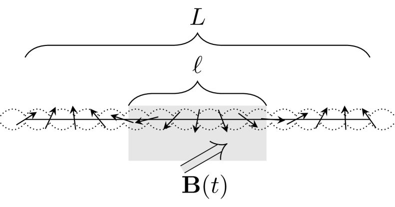
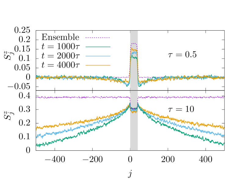
Figure 1: Above: System. A chain of $L$ classical spins, $l$ of which are subject to a uniform periodic magnetic field $\mathbf{B}(t)=\mathbf{B}(t+\tau)$. All spins have nearly isotropic nearest-neighbour interactions, with small disorder breaking conservation laws. Below: emerging states. The plots show a comparison between dynamical evolutions of the system over the time $t$ and predicted equilibrium expectation values of spatially resolved $z$-magnetisation. After a transient phase, both regimes may be described by effective Gibbs ensembles sampled via Monte Carlo techniques. For high frequencies, e.g. $\tau=0.5$, the driven sites (shaded region) locally see significant evolution. The reservoir, initialised in a thermal state with zero magnetisation, remains unchanged up to noise beyond a small correlation length. In contrast, the low-frequency profile, e.g. $\tau=10$, continues to spread deep into the reservoir at late times, indicating the global nature of the emerging steady state. We have set the parameters $L=2000$, $\ell=40$, $e_{\rm initial}=-0.66$, $\delta J=10^{-3}$, see Sec. II for details.

I Introduction

Floquet’s theorem states that any homogeneous system of linear differential equations with time-periodic coefficients can be mapped to an autonomous system by means of a linear basis transformation Floquet-1883 . This transformation carries the same periodicity as the original system an can be chosen to become the identity at integer multiples of the period. When applied to the Schrödinger equation this theorem implies that any periodically driven quantum system is connected by a time-periodic unitary transformation to an undriven system whose dynamics is stroboscopically equivalent Kitagawa-Oka-Brataas-Fu-Demler ; Sambe ; Torres-Kunold ; Bukov-DAlessio-Polkovnikov-review ; Eckardt-rmp . Classical equations of motion, however, are generally non-linear and there is indeed no intuitive counterpart to Floquet’s theorem in Hamiltonian mechanics, as can be seen from the following argument Anatoli-acknowledgement . Any autonomous classical system with one degree of freedom is integrable as energy provides the required conserved quantity. By extension, if it were always possible to find a time-periodic canonical transformation that renders its Hamiltonian time-independent, any periodically driven system with one degree of freedom would be integrable. This hypothesis is easily falsified by a counter-examples: Kapitza’s pendulum, for instance, is known to be non-integrable despite having only one degree of freedom Arnold ; Broer-Krauskopf ; Landau-Lifshitz .

This observation seems to leave us with a fundamental gap between quantum and classical mechanics. Indeed, driven by recent experimental advances KWW , studies of periodically driven many-body systems have so far mainly focused on the quantum regime, where Floquet theory has exposed a rich landscape of phenomena including sharp notions of non-equilibrium phases with no static counterpart Khemani-PRL ; Curt-phase , new perspectives on many-body quantum chaos Chalker-PRX , and the possibility of engineering specific band structures through precisely tunable driving fields Weitenberg-Simonet ; Rudner . Still, although there is no ‘classical Floquet theorem’, much of the methodology used to describe periodically driven quantum systems, such as the Floquet-Magnus expansion, formally extends to Hamiltonian systems. It is therefore not a priori obvious what phenomenology is particular to the quantum realm.

In fact, quantum and classical many-body systems are alike in that they generically tend to absorb energy from a periodic drive until they approach a trivial ‘infinite-temperature ensemble’ Ponte-Chandran-Papic-Abanin ; Lazarides-heating ; Russomanno-Silva-Santoro ; Ikeda-Polkovnikov . Some routes to avoid this overheating, such as preventing thermalisation through many-body localisation Curt-phase , draw on quantum effects. Others, like conservation laws Haldar-Das , may cause observables to synchronise thus giving rise to Gibbs ensembles with time-periodic Lagrange multipliers Lazarides-Das-Moessner-periodic ; or the high-frequency limit, where heating rates are typically exponentially suppressed in the driving frequency Abanin-DeRoeck-Ho-Huveneers ; Abanin-DeRoeck-Ho-Huveneers2 ; Abanin-DeRoeck-Huveneers ; Mori-Kuwahara-Saito ; Mori-Kuwahara-Saito2 ; should however be equally accessible in the classical regime.

This paper represents a contribution to a growing literature oriented around exploring the phenomenology of classical many-body systems Hodson-Jarzynski ; Howell ; Nunnenkamp ; McRoberts-Bilitewski-Haque-Moessner . We aim to shed new light on the so far relatively unexplored class of classical periodically driven many-body systems, which is potentially ripe with interesting physics. Furthermore, we set out to investigate how the dynamics of such a system can be stabilised away from the high-frequency limit by coupling to a large thermal reservoir. To these ends, we consider a classical spin-chain with nearest-neighbour interactions and weak disorder, a small fraction of which is subject to a time-periodic magnetic field, with the remainder acting as a reservoir, see Fig. 1. Expanding on our previous work short-paper , we simulate the full dynamics of this system and compare its emergent steady states with those predicted by Gibbs ensembles.

This analysis yields two major insights, which are exposed by the plots of Fig. 1. First, in the high-frequency regime, the driven part of the system quickly settles to a stroboscopic steady state with residual heat uptake being dissipated into the reservoir, which plays the rôle of a passive heat sink. This steady state is well described by a Gibbs ensemble, whose temperature is determined by the initial state of the reservoir. The corresponding effective Hamiltonian is accurately determined by the lowest orders of the classical Floquet-Magnus expansion, which is essentially a systematic method to average over the periodic driving, order by order in the inverse frequency. Second, even at low frequencies, the driven part of the system quickly attains a stroboscopic steady state, which survives well beyond initial transient behaviour and is only slowly destabilised by residual heating. Since, in contrast to the high-frequency regime, the driven spins can now follow the applied magnetic field, this state is characterised by synchronisation with the drive, which provides a new mechanism for the effective suppression of energy absorption. At the same time, the state of the reservoir is altered qualitatively as an emerging magnetisation profile spreads out from the driven sites and eventually covers the entire spin chain. This effect enables the redistribution of energy over large spatial distances and can be understood as a relaxation process in a rotating reference frame. In this picture, the entire system approaches a new Gibbs state, whose Hamiltonian differs from the original one throughout the driven and the undriven parts of the system. As a result, the corresponding effective temperature can deviate substantially from the initial temperature of the reservoir.

Thus, the two regimes are fundamentally different in nature. At high frequencies, the driven system dissipatively relaxes as if being locally quenched to a new Hamiltonian. At low frequencies, the driven system rapidly synchronises with the external magnetic field, while long-range correlations with the reservoir are established and a new global Gibbs state is gradually approached. Underpinned by profoundly different mechanisms, these two regimes are separated only by a narrow crossover region in frequency space. This crossover features a rapid change in the energy absorption of the system, and the scale for its onset is determined by the interaction strength between neighbouring spins short-paper .

Our analysis of this phenomenology proceeds as follows. In Sec. II we define the system and outline the numerical techniques for both dynamical simulation, and for statistical sampling of known distributions. In Sec. III we validate these numerical procedures for the undriven system, where we already have a firm theoretical footing in the standard results of statistical mechanics. Here, we set the scene for for the main quantities of interest. In Sec. IV we turn towards our main programme: investigating the periodically-driven dynamics of a classical many-body system. We approximately construct ensemble descriptions at both high and low frequencies, going beyond the leading order analysis of Ref. short-paper . We demonstrate that further corrections are indeed small and consistent with observed data. In Sec. V we investigate the behaviour of the reservoir itself, its importance in establishing the synchronisation of observables in the low-frequency ensemble, and comment on the non-Markovian nature of the system.

II System and simulation

II.1 Dynamics

The system under consideration, sketched in Fig. 1, comprises a chain of $L$ three-component classical spins ${\bf S}_{j}$ normalised such that $|{\bf S}_{j}|=1$. Its Hamiltonian is given by

$$\mathcal{H}(t)=-\sum_{j=1}^{L}{\bf S}_{j}^{\top}J_{j}^{\vphantom{\top}}{\bf S}_{j+1}^{\vphantom{\top}}+\sum_{j=1}^{\ell}{\bf B}(t)\cdot{\bf S}_{j},$$ (1)

where we assume periodic boundary conditions ${\bf S}_{L+1}={\bf S}_{1}$. The rotating magnetic field ${\bf B}(t)=\left(\cos(\omega t),\sin(\omega t),0\right)^{\top}$, with period $\tau=2\pi/\omega$, acts on the sites $j=1,\ldots,\ell$, to which we refer as the ‘system proper’. Accordingly, we call the undriven $L-\ell$ sites the ‘reservoir’. The coupling matrices are diagonal $J_{j}={\rm diag}[J_{j}^{x},J_{j}^{y},J_{j}^{z}]$. To break any exact conservation laws constraining the dynamics, we choose the $J_{j}^{\alpha}$ independently and identically distributed from a normal distribution, with mean $J$ which we set equal to $1$ throughout, and variance $\delta J$ i.e. $J_{j}^{\alpha}\sim\mathcal{N}(1,\delta J)$. To match the dimensions of energies and frequencies, we formally set the reduced Planck constant $\hbar$ equal to 1, hence the spins being dimensionless.

The equations of motion are determined by the Poisson bracket $\{S_{j}^{\alpha},S_{k}^{\beta}\}=\delta_{jk}\varepsilon^{\alpha\beta\gamma}S_{j}^{\gamma}$ via Hamilton’s equations

$$\frac{\mathrm{d}{\bf S}_{j}}{\mathrm{d}t}=\{\mathcal{H}(t),{\bf S}_{j}\}.$$ (2)

This rule yields a coupled system of non-linear differential equations for the spin degrees of freedom,

$$\frac{\mathrm{d}{\bf S}_{j}}{\mathrm{d}t} =-{\boldsymbol{\Omega}}_{j}\times{\bf S}_{j},$$ (3)

$${\boldsymbol{\Omega}}_{j} =J_{j-1}{\bf S}_{j-1}+J_{j}{\bf S}_{j+1}-\begin{cases}{\bf B}(t),&1\leq j\leq\ell,\\ 0,&{\rm otherwise}\end{cases}.$$

If the applied field ${\bf B}$ were to vanish and all $J_{j}$ were the identity matrix, the total magnetisation $\boldsymbol{\mathcal{M}}=\frac{1}{L}\sum_{j=1}^{L}{\bf S}_{j}$ would be an exactly conserved quantity. To apply the principles of statistical mechanics, we would then have to include these additional conserved quantities through Lagrange multipliers determined by the initial conditions, and any statistical sampling would have to respect this constraint. We add a small amount of Gaussian noise to the couplings $J_{j}$ to preclude such fine-tuning. This disorder breaks all conservation laws, and even in the absence of driving only energy conservation holds, but does not significantly affect the macroscopic properties of the system otherwise.

To fully determine the dynamics, we now specify the initial conditions for the equations of motion (3). To understand the general behaviour of the system, we take a statistical approach rather than focusing on individual trajectories, which may be subject to fluctuations. Our initial states are therefore drawn from a Gibbs ensemble defined by

$$\mathcal{P}_{0} =e^{-\beta\mathcal{H}_{0}}/\mathcal{Z}_{0},$$ (4)

$$\mathcal{H}_{0} =-\sum_{j=1}^{L}{\bf S}_{j}^{\top}J_{j}^{\vphantom{\top}}{\bf S}_{j}^{{\vphantom{\top}}},$$

with $\beta$ being an inverse temperature chosen to fix a specific initial mean energy density, and $\mathcal{Z}_{0}$ being a normalisation constant. With these initial conditions, the system would remain statistically invariant under its time evolution if no magnetic field were applied. Hence, when the field is applied to the system proper, the dynamics of the reservoir are locally in equilibrium and we do not need to account for quench-like effects. We expect both the slow and fast driving regimes to result in minimal energy absorption, and that the state of the reservoir is only gradually modified. In the following, unless otherwise indicated, all presented results correspond to averages over both initial conditions and realisations of disorder for $J_{j}$.

II.2 Numerical techniques

As given by Eq. (3), the instantaneous evolution of each spin ${\bf S}_{j}$ is a rotation in an effective magnetic field determined by the on-site magnetic field and the field from its nearest neighbours ${\bf S}_{j-1}$ and ${\bf S}_{j+1}$. The dynamics of the spin-chain may therefore be efficiently simulated using alternated updating Jin-et-al . The basic idea of this approach is to split the spin-chain into two interleaving sub-chains $A$ and $B$ comprising the even and odd sites, respectively. The local field for each spin in $A$ depends only on those in $B$, and vice versa, and we can update these fields alternately. More precisely, the technique we implement is drawn from Refs. Jin-et-al ; Krech-Bunker-Landau and uses the simplest Suzuki-Trotter decomposition of the time-evolution operator from time $t$ to $t+\delta t$, $U(t+\delta t,t)$. That is, we have

$$U(t+\delta t,t)=e^{\frac{\delta t}{2}\mathcal{L}^{A}_{t+\delta t/2}}e^{\delta t\mathcal{L}^{B}_{t+\delta t/2}}e^{\frac{\delta t}{2}\mathcal{L}^{A}_{t+\delta t/2}}+\mathcal{O}(\delta t^{3}).$$ (5)

The Liouville operator $\mathcal{L}^{A/B}_{t+\delta t/2}$ generates rotations on the sub-chain $A/B$ in the effective field determined from sub-chain $B/A$ at time $t+\delta t/2$. The error of this decomposition is bounded by terms of order $\delta t^{3}$. As the propagation over a time step $\delta t$ is now formulated solely in terms of rotations, the spin normalisation is manifestly preserved by this procedure.

We will make extensive use of Monte Carlo (MC) techniques to sample from particular Gibbs distributions. We use standard Metropolis-Hastings sampling, where a site is chosen randomly with equal probability, and a proposed update of the spin at the particular site pointing in a new direction chosen uniformly from the surface of the unit sphere. The proposed update is then accepted if the energy of the new configuration decreases i.e. $\Delta E\leq 0$, or accepted with probability $e^{-\beta\Delta E}$ if $\Delta E>0$. As the number of proposals accepted/rejected increases, this procedure is asymptotically guaranteed to sample from the Gibbs ensemble Newman-Barkema .

III Undriven system

To set the stage for our main investigations and to confirm the validity of our numerical approach, we first consider the undriven system, reproducing results from Ref. [Jin-et-al, ]. That is, we set ${\bf B}=0$ so that the Hamiltonian of the entire spin chain is given by $\mathcal{H}_{0}$ of Eq. (4). We initialise the entire spin chain in a random state with a fixed mean energy and zero total magnetisation, which then evolves under the equations of motion (3). The fundamental postulate of statistical mechanics asserts that time averages and ensemble averages are equivalent in an ergodic system. This equivalence extends to all moments of observables, and therefore their full distributions.

In a canonical ensemble with inverse temperature $\beta$ the probability distribution of any observable $\hat{O}=\hat{O}(\{{\bf S}_{j}\})$ reads

$$P_{\rm can}(O)=\frac{1}{\mathcal{Z}_{0}}\int\mathrm{d}{\bf S}_{1}\ldots\mathrm{d}{\bf S}_{L}e^{-\beta\mathcal{H}_{0}}\delta\left[O-\hat{O}(\{{\bf S}_{j}\})\right],$$ (6)

with $\mathcal{Z}_{0}$ being a normalisation, which sums the probability of all configurations compatible with $\hat{O}=O$. Note that we use the canonical ensemble as a matter of convenience throughout. This approach should be equivalent to a microcanonical one up to finite-size corrections.

To confirm that the undriven spin chain satisfies ergodicity, we compute the full probability distributions of macroscopic observables over a single trajectory and compare them with the corresponding ensemble distribution (6). For an arbitrary observable $\hat{O}$, we may sample at times $t_{1},\ldots,t_{\mathcal{N}}$, and write the binned probability density with bin width $\epsilon$ as

$$P_{T}(O)=\frac{1}{\mathcal{N}}\sum_{n=1}^{\mathcal{N}}\Pi_{\epsilon}\left[O-\hat{O}(\{{\bf S}_{j}(t_{n})\})\right],$$ (7)

where the sample times are given by $t_{n}=t_{0}+n\Delta t$, choosing $t_{0}$, $\Delta t$, and $\mathcal{N}$ sufficiently large such that the result is insensitive to specific values. The function $\Pi_{\epsilon}$ counts the number of points along the trajectory, where the value of $\hat{O}$ lies within the window of width $\epsilon$ centred at $O$. In other words, $\Pi_{\epsilon}$ is an approximation of a delta-function, formally given by

$$\Pi_{\epsilon}[x]=\frac{1}{\epsilon}\begin{cases}1&-\epsilon/2\leq x\leq\epsilon/2\\ 0&{\rm otherwise}\end{cases}.$$ (8)

MC sampling is a numerical technique that generates samples in the correct proportions as determined by a given probability distribution, without having to exhaustively explore the phase space of the system. We may therefore construct the ensemble distribution (6) for any observable by using $M$ MC samples as outlined in Sec. II.2. Specifically, the equivalent of Eq. (7) for the Gibbs ensemble is

$$P_{{\rm can}}(O)=\frac{1}{M}\sum_{m=1}^{M}\Pi_{\epsilon}\left[O-\hat{O}(\{{\bf S}_{j}^{(m)}\})\right],$$ (9)

where ${\bf S}_{j}^{(m)}$ is the $m$th MC sample. We note that the MC algorithm samples from the canonical ensemble, and due to energy conservation the dynamical trajectory is sampling from the microcanonical ensemble. However, when comparing local observables involving only degrees of freedom of the first $\ell\ll L$ sites, even the energy density will fluctuate, and the equivalence of ensembles implies that all results should be identical up to finite-size effects.

In Fig. 2, we show that single-trajectory and ensemble distributions are in excellent agreement for the representative observables

$${\bf m} =\frac{1}{\ell}\sum_{j=1}^{\ell}{\bf S}_{j},$$ (10)

$$e =-\frac{1}{\ell-1}\sum_{j=1}^{\ell-1}{\bf S}_{j}^{\top}J^{\vphantom{\top}}_{j}{\bf S}^{\vphantom{\top}}_{j+1},$$

i.e. the magnetisation and energy density of the system proper. This result confirms that the undriven system behaves ergodically even if $\delta J=10^{-3}$ is small.

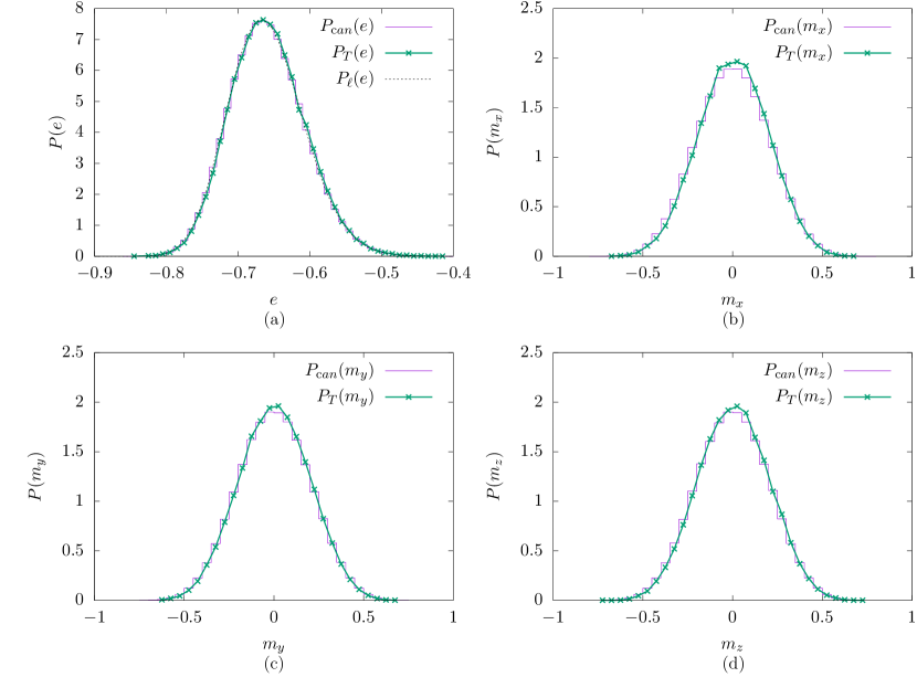
Figure 2: Undriven system. Histograms showing $P_{T}(O)$ of Eq. (7) determined from one trajectory with $\mathcal{N}=64000$ samples (crosses), compared with $P_{\rm can}(O)$ of Eq. (9), where each Monte-Carlo curve is binned from $M=64000$ samples. The shown observables are (a) energy density, (b) $x$-magnetisation, (c) $y$-magnetisation, (d) $z$-magnetisation. For all plots, we have set $L=2000$, $\ell=40$, $\delta J=2\times 10^{-3}$, and chosen the energy density of the entire system $e_{\rm initial}=-0.66$, which implicitly fixes the inverse temperature $\beta$ for the MC simulation. The exact result (dashed line) of Eq. (15) is also shown in (a).

For the isotropic chain, $\delta J=0$, we may also compute the exact probability distribution for the energy density at large $\ell$. We here consider open boundary conditions, which are equivalent to periodic boundary conditions up to finite-size corrections. Firstly, the partition function is given by

$$Z=\int\mathrm{d}{\bf S}_{1}\cdots\mathrm{d}{\bf S}_{\ell}\,e^{\beta\sum_{j=1}^{\ell-1}{\bf S}_{j}\cdot{\bf S}_{j+1}},$$ (11)

where $\mathrm{d}{\bf S}_{j}=\frac{1}{4\pi}\sin\theta_{j}\mathrm{d}\theta_{j}\mathrm{d}\phi_{j}$ indicates integration over the spherical angles of each spin. Rewriting this expression in terms of the angle between adjacent spins in the chain we find

$$Z=\left[\frac{1}{2}\int_{-1}^{1}\mathrm{d}\cos\theta e^{\beta\cos\theta}\right]^{\ell-1}=\left(\frac{\sinh\beta}{\beta}\right)^{\ell-1}.$$ (12)

Hence, the free energy density of the isotropic chain at inverse temperature $\beta$ is given by Parsons

$$f(\beta)=-\frac{1}{\beta(\ell-1)}\ln Z=-\frac{1}{\beta}\ln\frac{\sinh\beta}{\beta}.$$ (13)

We may thus calculate the probability distribution for the energy density $e$ of Eq. (10) as

$$P(e) =\frac{1}{Z}\int\mathrm{d}{\bf S}_{1}\cdots\mathrm{d}{\bf S}_{\ell}e^{\beta\sum_{j=1}^{\ell-1}{\bf S}_{j}\cdot{\bf S}_{j+1}}$$ (14)

$$\int_{-\infty}^{\infty}\frac{\mathrm{d}z}{2\pi}e^{iz\left(e(\ell-1)+\sum_{j=1}^{\ell-1}{\bf S}_{j}\cdot{\bf S}_{j+1}\right)},$$

where we have used the Fourier representation of the Dirac delta function appearing in Eq. (6). Employing the method of steepest descent erdelyi , this integral may be approximated as

$$P_{\ell}(e)=\frac{\mathcal{Q}}{\sqrt{(\ell-1)|g^{\prime\prime}(z^{*})|}}e^{-(\ell-1)g(z^{*})},$$ (15)

where $\mathcal{Q}$ is a normalisation constant, and $\beta$ is chosen to fix the mean energy density $\frac{1}{\beta}-\coth\beta=\langle e\rangle$. The function $g(z)=(\beta-z)f(\beta-z)+ez$ determines the saddle-point, which is given by $z^{*}$ such that $g^{\prime}(z^{*})=0$. Fig. 2(a) shows that the exact distribution (15) agrees well with both numerical approaches. This result confirms weak disorder $\delta J\ll 1$ eliminates conservation laws but has no visible effect on the distributions of macroscopic observables.

IV Driven system

Having established that the undriven system is ergodic, we now turn to the effect of periodic driving. Our basic expectations are as follows: at high frequencies, the driving ‘averages out’ and the dynamics are described by the Hamiltonian with no applied field $\mathcal{H}_{0}$ of Eq. (4); at very low frequencies, the system relaxes to the instantaneous Hamiltonian. Here, we develop these expectations into quantitative descriptions of the two regimes, which we show to predict the behaviour of the system over a remarkably wide range of frequencies short-paper .

IV.1 High frequency

Intuitively, the physics at high frequencies should be well approximated by the averaged Hamiltonian. This intuition is captured by the Floquet-Magnus expansion. This technique proceeds by assuming that a time-independent generator for the stroboscopic dynamics does exist, and then constructs it order-by-order in the driving period Blanes-Casas-Oteo-Ros . The Floquet-Magnus expansion was originally devised for linear systems, and is expansively used for the description of periodically-driven quantum systems. It can, however, be adapted to classical Hamiltonian systems, whose dynamics are non-linear, by formally treating the Poisson bracket as a linear operator. That is, we write the equations of motion for a phase-space observable of the isolated system proper, $\hat{O}({\bf S}_{1},\ldots,{\bf S}_{\ell})$, in the form

$$\frac{\mathrm{d}\hat{O}(t)}{\mathrm{d}t}=\mathcal{L}_{H(t)}\hat{O}(t),$$ (16)

where $\mathcal{L}_{H(t)}\cdot=\{H(t),\cdot\}$ denotes the Liouville operator and

$$H(t)=-\sum_{j=1}^{\ell-1}{\bf S}_{j}^{\top}J^{\vphantom{\top}}_{j}{\bf S}_{j+1}^{\vphantom{\top}}+\sum_{j=1}^{\ell}{\bf B}(t)\cdot{\bf S}_{j}$$ (17)

is the Hamiltonian of the driven system proper. If the Floquet theorem were to hold, the formal solution of Eq. (16) at $t=n\tau$ would take the form

$$\hat{O}(n\tau)=e^{n\tau\mathcal{L}_{H_{F}}}\hat{O}(0),$$ (18)

where $H_{F}$ would be the Floquet Hamiltonian. While such an object does not exist in general, it can still be perturbative constructed close to the infinite frequency limit $\tau\to 0$, where $H_{F}\to\frac{1}{\tau}\int_{0}^{\tau}\mathrm{d}tH(t)$. To this end, we introduce the dimensionless time $s=t/\tau$ and make the ansatz

$$\hat{O}^{\prime}(s)=\hat{O}(s\tau)=e^{\mathcal{L}_{K(s)}}\hat{O}^{\prime}(s),$$ (19)

with $0\leq s\leq 1$ and the Magnus Hamiltonian

$$K(s)=\sum_{n=0}^{\infty}\tau^{n}K^{(n)}(s).$$ (20)

Upon inserting this ansatz into the equation of motion for $\hat{O}^{\prime}(s)$ and following the formal steps of the conventional Magnus expansion Kitagawa-Oka-Brataas-Fu-Demler , $K(s)$ can be determined order by order. Returning to original units then yields the effective Floquet Hamiltonian

$$H_{F}=\frac{1}{\tau}K(t=\tau)=\sum_{n=0}^{\infty}H_{F}^{(n)},$$ (21)

where the first few terms are given by

$$H_{F}^{(0)} =\frac{1}{\tau}\int_{0}^{\tau}\mathrm{d}t\,H(t),$$ (22)

$$H_{F}^{(1)} =\frac{1}{2!\tau}\int_{0}^{\tau}\mathrm{d}t_{1}\int_{0}^{t_{1}}\mathrm{d}t_{2}\,\{H(t_{1}),H(t_{2})\},$$

$$H_{F}^{(2)} =\frac{1}{3!\tau}\int_{0}^{\tau}\mathrm{d}t_{1}\int_{0}^{t_{1}}\mathrm{d}t_{2}\int_{0}^{t_{2}}\mathrm{d}t_{3}\,$$

$$\left\{H(t_{1}),\{H(t_{2}),H(t_{3})\}\right\}$$

$$+\left\{H(t_{3}),\{H(t_{2}),H(t_{1})\}\right\}.$$

This expansion can in general only be expected to be asymptotic Bender-Orszag ; Berry ; mori-floquet-prethermal , and one usually truncates the sum in Eq. (21) after the first few terms.

Evaluating the first two expressions explicitly, we find

$$H_{F}^{(0)} =-\sum_{j=1}^{L}{\bf S}^{\top}_{j}J_{j}^{\vphantom{\top}}{\bf S}^{\vphantom{\top}}_{j+1},$$ (23)

$$H_{F}^{(1)} =-\frac{1}{\omega}\sum_{j=1}^{\ell}\left(\frac{1}{2}S_{j}^{z}+\hat{\bf y}\cdot({\boldsymbol{\Omega}_{j}}\times{\bf S}_{j})\right).$$

Noting that $H_{F}^{(0)}$ is equal to the Hamiltonian of the initial ensemble Eq. (4), we must consider at least the first order in $\tau$ of the Floquet-Magnus expansion to observe deviations from the initial state. In our previous work the corrections from $H_{F}^{(1)}$ were observable and consistent with the true dynamics for $\tau\lesssim 1$ short-paper . For clarity, we may write

$$H_{F}^{(n)}=h_{\rm SB}^{(n)}+h_{\rm MB}^{(n)},$$ (24)

where $h_{\rm SB}^{(n)}$ accounts for single body terms, and $h_{\rm MB}^{(n)}$ accounts for many-body terms. Accordingly,

$$h_{\rm SB}^{(1)} =-\frac{1}{2\omega}\sum_{j=1}^{\ell}\frac{1}{2}S_{j}^{z},$$ (25)

$$h_{\rm MB}^{(1)} =-\frac{\hat{\bf y}}{\omega}\cdot\sum_{j=1}^{\ell}{\boldsymbol{\Omega}_{j}}\times{\bf S}_{j}.$$

It is interesting to ask if including higher-order corrections from $H_{F}^{(2)}$ improves the results of Ref. short-paper further. Calculating $H_{F}^{(2)}=h_{\rm SB}^{(2)}+h_{\rm MB}^{(2)}$ yields

$$h_{\rm SB}^{(2)} =\frac{1}{2\omega^{2}}\sum_{j=1}^{\ell}S_{j}^{x},$$ (26)

$$h_{\rm MB}^{(2)} =\frac{1}{2\omega^{2}}\sum_{j=1}^{\ell}\left\{2\hat{\bf x}\cdot\left[{\boldsymbol{\Omega}}_{j}\times\left({\boldsymbol{\Omega}}_{j}\times{\bf S}_{j}\right)\right.\right.$$

$$\left.\left.+\left(J_{j-1}\left({\boldsymbol{\Omega}}_{j-1}\times{\bf S}_{j-1}\right)+J_{j}\left({\boldsymbol{\Omega}}_{j+1}\times{\bf S}_{j+1}\right)\right)\times{\bf S}_{j}\right]\right.$$

$$\left.+\frac{1}{2}\left(3\Omega^{x}_{j}S_{j}^{x}+\Omega_{j}^{y}S_{j}^{y}-J_{j-1}^{y}S_{j}^{z}S_{j-1}^{z}\right.\right.$$

$$\left.\left.-J_{j}^{y}S_{j}^{z}S_{j+1}^{z}-J_{j-1}^{z}S_{j}^{y}S_{j-1}^{y}-J_{j}^{z}S_{j}^{y}S_{j+1}^{y}\right.\right.$$

$$\left.\left.-3J_{j-1}^{x}S_{j}^{z}S_{j-1}^{z}-3J_{j}^{x}S_{j}^{z}S_{j+1}^{z}\right.\right.$$

$$\left.\left.-3J_{j-1}^{z}S_{j}^{x}S_{j-1}^{x}-3J_{j}^{z}S_{j}^{x}S_{j+1}^{x}\right)\right\}.$$

The single-body terms $h_{\rm SB}^{(n)}$ constitute the Floquet-Magnus expansion under the free Hamiltonian $H_{\rm free}=\sum_{j=1}^{\ell}{\bf B}(t)\cdot{\bf S}_{j}$, a linear system for which the expansion may be resummed to yield the effective field of the rotating frame ${\bf B}_{\rm rot}=\hat{\bf x}-\omega\hat{\bf z}$ feldman . The many-body terms have more complex structure and become increasingly non-local at each subsequent order.

Assuming that the stroboscopic dynamics of the system proper is asymptotically equivalent to the autonomous dynamics of the associated Floquet system, we may define the $N$th order Floquet-Magnus ensemble by

$$P_{F}^{(N)}=\frac{1}{Z_{F}^{(N)}}\exp\left(-\beta\sum_{n=0}^{N}H_{F}^{(n)}\right),$$ (27)

where $Z_{F}^{(N)}$ accounts for normalisation. As we expect absorption to be exponentially small in $\omega$ at high frequencies rubio-abadal , we neglect heating and assume the temperature of the ensemble to be well approximated by that of the initial state defined by Eq. (4). As may be seen in Fig. 3, including additional terms in the Magnus ensemble beyond $N=1$ produces only minimal improvement on the previously observed results at $\tau=0.5$. We can thus conclude that the two lowest orders of the Floquet-Magnus expansion are indeed sufficient to describe the stroboscopic steady state of the system proper, even well away from the infinite-frequency limit.

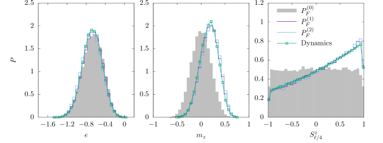
Figure 3: High-frequency picture. Histogram distributions for $\tau=0.5$ of the energy density and $z$-magnetisation of the system proper, $e$ and $m_{z}$, and the $z$-component of the spin at site $f=\ell/4$, $S^{z}_{\ell/4}$, in the $N$th order Floquet-Magnus ensembles as defined by Eq. (27) for $N=0,1,2$ compared with dynamical evaluations. Statistical ensembles are sampled according to Eq. (9), and the dynamical ones according to Eq. (7) using multiple trajectories and choosing $t_{0}$ long enough for observables to relax. For all plots, we have set $L=2000$, $\ell=40$, $\delta J=0.02$, and chosen the initial energy density $e_{\rm initial}=-0.66$, which fixes the inverse temperature $\beta$ for the MC simulation. Due to the minimal energy absorption, we sample multiple points from each trajectory after a transient period to improve statistics. Here we sample 4000 points each from 200 separate trajectories, from the interval $t=6000\tau$ to $t=10,000\tau$.

IV.2 Low frequency

IV.2.1 Leading order

The results of the previous section show that the high-frequency regime can be fully described in a local picture focusing only on the system proper and treating the reservoir as a passive heat sink. To understand the low-frequency regime, we must adopt a global picture, where both system proper and reservoir are affected by the driving. This approach is motivated by the observation that the stroboscopic dynamics of the full system are nearly equivalent to the dynamics of an autonomous Floquet system for sufficiently small $\delta J$ but arbitrary $\omega$. Specifically, upon introducing the rotating-frame variables

$$\widetilde{\bf S}_{j}=\begin{pmatrix}\cos(\omega t)&\sin(\omega t)&0\\ -\sin(\omega t)&\cos(\omega t)&0\\ 0&0&1\end{pmatrix}{\bf S}_{j},$$ (28)

the equations of motion (3) may be recast as

$$\frac{\mathrm{d}\widetilde{\bf S}_{j}}{\mathrm{d}t} =-\widetilde{\boldsymbol{\Omega}}_{j}\times\widetilde{\bf S}_{j}+\mathcal{O}(\delta J),$$ (29)

$$\widetilde{\boldsymbol{\Omega}}_{j} =-(\bar{J}_{j-1}\widetilde{\bf S}_{j-1}+\bar{J}_{j}\widetilde{\bf S}_{j+1})$$

$$-\omega\hat{\bf z}+\begin{cases}\hat{\bf x},&1\leq j\leq\ell,\\ 0,&{\rm otherwise}\end{cases}.$$

Thus, upon neglecting time-dependent terms of order $\delta J$, the dynamics in the rotating frame are generated by the time-independent Hamiltonian

$$\mathcal{H}_{\rm rot}=-\sum_{j=1}^{L}\left(\widetilde{\bf S}_{j}^{\top}\bar{J}_{j}^{\vphantom{\top}}\widetilde{\bf S}_{j+1}^{\vphantom{\top}}+\omega\hat{\bf z}\cdot\widetilde{\bf S}_{j}\right)+\sum_{j=1}^{\ell}\hat{\bf x}\cdot\widetilde{\bf S}_{j},$$ (30)

where $\bar{J}_{j}={\rm diag}\left[\frac{1}{2}\left(J_{j}^{x}+J_{j}^{y}\right),\frac{1}{2}\left(J_{j}^{x}+J_{j}^{y}\right),J_{j}^{z}\right]$.

This result shows that the observable $\mathcal{H}_{\rm rot}$, which plays the rôle of a global Floquet Hamiltonian, is nearly conserved in the rotating frame. At the same time $\mathcal{H}_{\rm rot}$ is a sum of local densities. Hence, by usual arguments of statistical mechanics, the entire system should relax to an ensemble of the form

$$\mathcal{P}_{\rm rot}=e^{-\beta_{\rm rot}\mathcal{H}_{\rm rot}}/\mathcal{Z}_{\rm rot}.$$ (31)

Note that formally, the system should be described by a microcanonical ensemble. However, for all local observables the canonical ensemble above should provide an equivalent description up to finite size effects.

The effective inverse temperature $\beta_{\rm rot}$ may now be determined from the fact that $\mathcal{H}_{\rm rot}$ is an almost conserved quantity: assuming that the system has fully relaxed to the ensemble described by Eq. (31), and that persistent heating has only minor effects, the mean value of $\mathcal{H}_{\rm rot}$ in the initial state $\mathcal{P}_{0}$ of Eq. (4) should be nearly identical to its mean value in the steady state of Eq. (31). That is, the equation

$$\int\mathrm{d}{\bf S}_{1}\cdots\mathrm{d}{\bf S}_{L}\mathcal{H}_{\rm rot}\mathcal{P}_{0}=\int\mathrm{d}{\bf S}_{1}\cdots\mathrm{d}{\bf S}_{L}\mathcal{H}_{\rm rot}\mathcal{P}_{\rm rot},$$ (32)

implicitly fixes $\beta_{\rm rot}$ according to standard arguments of statistical mechanics. Upon integrating out the reservoir degrees of freedom in Eq. (31), we thus find the effective stroboscopic ensemble

$$P_{\rm rot}=\frac{1}{Z_{\rm rot}}e^{-\beta_{\rm rot}^{\rm stat}H_{\rm rot}},$$ (33)

where $Z_{\rm rot}$ is a normalisation and now the rotating frame Hamiltonian is, up to $\delta J$ corrections and boundary effects,

$$H_{\rm rot}=-\sum_{j=1}^{\ell-1}\widetilde{\bf S}_{j}^{\top}\bar{J}_{j}^{\vphantom{\top}}\widetilde{\bf S}_{j+1}^{\vphantom{\top}}+\sum_{j=1}^{\ell}\left(\hat{\bf x}-\omega\hat{\bf z}\right)\cdot\widetilde{\bf S}_{j}^{\vphantom{\top}}.$$ (34)

As reported in Ref. [short-paper, ], the ensemble of Eq. (33) yields excellent results for the distribution of system-proper observables at very low frequencies e.g. $\tau=10$. For higher frequencies, however, we find in Fig. 4 that these ensemble distributions deviate significantly from the dynamical ones. Notably, however, the ensemble of Eq. (33) still reproduces the dynamical distributions accurately if $\beta_{\rm rot}^{\rm stat}$ is replaced with some $\beta_{\rm rot}=\beta_{\rm rot}^{*}<\beta_{\rm rot}^{\rm stat}$, which can be found by fitting only the mean energy density of the system proper. These discrepancies highlight the limitations of the assumptions made in writing down Eq. (32), which we explore further in Sec. V.

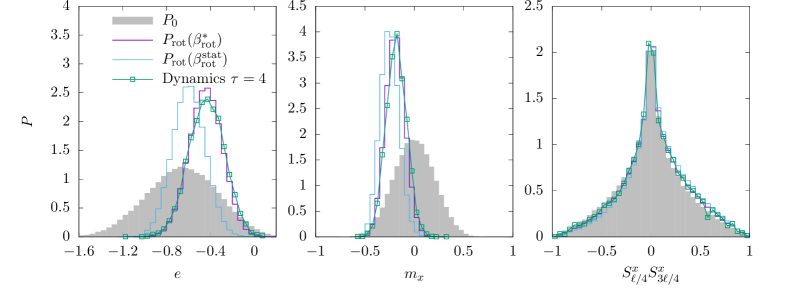
Figure 4: Low-frequency picture. Histogram distributions for observables of the system proper at $\tau=4$: comparing $\mathcal{N}=6000$ dynamical evolutions sampled at $t=1000\tau$, with $M=256,000$ MC samples from ensemble of Eq. (33) for both $\beta_{\rm rot}=\beta_{\rm rot}^{\rm stat}$ and best fit $\beta_{\rm rot}^{*}$. For reference, the initial ensemble $P_{0}$ of Eq. (4) is shown in grey. From left to right, the plots show energy density, $x$-magnetisation density, and a two-point spatial correlations function of the $x$-components of the spins at $j=\ell/4$ and $j=3\ell/4$. Here we have set $\ell=40$, $L=4000$, $\delta J=10^{-3}$, $e_{\rm initial}=-0.66$.

IV.2.2 Higher order corrections

We have so far discarded corrections in $\delta J$, assuming their effects are perturbatively small, but did not yet justify this simplification. In the case of high-frequency driving, the Magnus expansion provides a controlled scheme where corrections are asymptotically small in $\tau$. This technique can still be applied in the low-frequency regime to obtain systematic corrections to the leading-order picture discussed above. To this end, we observe that the full equations of motion, retaining corrections neglected in Eq. (29), in the rotating frame are given by

$$\frac{\mathrm{d}\widetilde{\bf S}_{j}}{\mathrm{d}t} =-(\bar{J}_{j-1}\widetilde{\bf S}_{j-1}+\bar{J}_{j}\widetilde{\bf S}_{j+1})\times\widetilde{\bf S}_{j}$$ (35)

$$-(\delta{J}_{j-1}(t)\widetilde{\bf S}_{j-1}+\delta{J}_{j}(t)\widetilde{\bf S}_{j+1})\times\widetilde{\bf S}_{j}$$

$$+\left\{\begin{array}[]{lr}\hat{\bf x}-\omega\hat{\bf z},&{\rm if}\ 1\leq j\leq\ell,\\ -\omega\hat{\bf z},&{\rm if}\ \ell<j\leq L\end{array}\right\}\times\widetilde{\bf S}_{j},$$

where

$$\bar{J}_{j} =\begin{pmatrix}\frac{1}{2}\left(J_{j}^{x}+J_{j}^{y}\right)&0\\ 0&\frac{1}{2}\left(J_{j}^{x}+J_{j}^{y}\right)&0\\ 0&0&J_{j}^{z}\end{pmatrix},$$ (36)

$$\delta J_{j}(t) =\frac{\Delta J_{j}}{2}\begin{pmatrix}-\cos(2\omega t)&\sin(2\omega t)&0\\ \sin(2\omega t)&\cos(2\omega t)&0\\ 0&0&0\end{pmatrix},$$

$$\Delta J_{j} =J_{j}^{y}-J_{j}^{x}.$$

These equations of motion are generated by the Hamiltonian

$$\mathcal{H}_{\rm rot}(t) =-\sum_{j=1}^{L}\left[\widetilde{\bf S}_{j}^{\top}\left(\bar{J}_{j}^{\vphantom{\top}}+\delta J_{j}^{\vphantom{\top}}(t)\right)\widetilde{\bf S}_{j+1}^{\vphantom{\top}}+\omega\hat{\bf z}\cdot\widetilde{\bf S}_{j}^{\vphantom{\top}}\right]$$ (37)

$$+\sum_{j=1}^{\ell}\hat{\bf x}\cdot\widetilde{\bf S}_{j}^{\vphantom{\top}}.$$

We see that time-dependent corrections are formally of order $\delta J$. Whilst we are not in the high-frequency regime, we nonetheless have an energy scale parametrically smaller than the driving frequency $\omega\gg\delta J$. Thus, over the course of one cycle of the drive, we can average over the dynamics induced by the oscillating contributions proportional to $\delta J$. That is, we may employ the Floquet-Magnus expansion in the rotating frame, which will generate an asymptotic series in powers of $\delta J/\omega$.

After some algebra, we find the first order global Floquet Hamiltonian in the rotating frame,

$$\mathcal{H}_{F}^{\rm rot} =\mathcal{H}_{\rm rot}^{(0)}+\mathcal{H}_{\rm rot}^{(1)}+\mathcal{O}(\tau^{2}),$$ (38)

$$\mathcal{H}_{\rm rot}^{(0)} =-\sum_{j=1}^{L}\left(\widetilde{\bf S}_{j}^{\top}J_{j}^{\vphantom{\top}}\widetilde{\bf S}_{j+1}^{\vphantom{\top}}+\omega\hat{\bf z}\cdot\widetilde{\bf S}_{j}^{\vphantom{\top}}\right)+\sum_{j=1}^{\ell}\hat{\bf x}\cdot\widetilde{\bf S}_{j}^{\vphantom{\top}},$$

$$\mathcal{H}_{\rm rot}^{(1)} =-\frac{1}{16\omega}\sum_{j=1}^{L}\left\{\Delta J_{j}\Delta J_{j}\left(\sigma^{z}\widetilde{\bf S}_{j}\right)\cdot\left(\sigma^{x}\widetilde{\bf S}_{j}\right)\times\widetilde{\bf S}_{j+1}\right.$$

$$\left.+\Delta J_{j-1}\Delta J_{j-1}\left(\sigma^{z}\widetilde{\bf S}_{j}\right)\cdot\left(\sigma^{x}\widetilde{\bf S}_{j}\right)\times\widetilde{\bf S}_{j-1}\right.$$

$$\left.+\Delta J_{j-1}\Delta J_{j}\widetilde{\bf S}_{j}\cdot\left[\left(\sigma^{z}\widetilde{\bf S}_{j+1}\right)\times\left(\sigma^{x}\widetilde{\bf S}_{j-1}\right)\right.\right.$$

$$\left.\left.-\left(\sigma^{x}\widetilde{\bf S}_{j+1}\right)\times\left(\sigma^{z}\widetilde{\bf S}_{j-1}\right)\right]\right\},$$

where we have introduced the matrices

$$\sigma^{z}=\begin{pmatrix}1&0&0\\ 0&-1&0\\ 0&0&0\end{pmatrix},\qquad\sigma^{x}=\begin{pmatrix}0&1&0\\ 1&0&0\\ 0&0&0\end{pmatrix}.$$ (39)

It is natural to ask whether we can distinguish these corrections coming from $\mathcal{H}_{\rm rot}^{(1)}$ at the level of non-equilibrium ensembles. Upon recalling that $\Delta J_{j}\sim\delta J$, one would expect the expansion to have a leading contribution with a pre-factor $\delta J/\omega$, which we would expect to be distinguishable in distributions of observables. For the specific drive considered, however, we see from Eq. (38) that these corrections vanish and the leading terms are in fact of order $(\delta J)^{2}/\omega$. Hence, for any practically relevant frequency regime, higher-order corrections may be safely neglected.

V Nature and rôle of the reservoir

Here we expand on the rôle that the reservoir plays in stabilising the stroboscopic non-equilibrium steady states constructed in Section IV. We first demonstrate how finite disorder rapidly causes runaway heating in the bare driven system away from high frequencies. Coupling a reservoir establishes a channel for heat transport away from the driven sites. Thus, at high frequencies, residual heating is compensated by dissipation with the reservoir acting as a nearly reversible heat sink.

At low frequencies, however, the state of the reservoir is altered on a macroscopic scale, while the spins of the system proper synchronise with the drive. This effect suppresses the net heat uptake of the entire spin chain and stabilises a non-trivial steady state of the system proper at low and intermediate frequencies. To corroborate this picture, we evaluate spatially resolved observables and explore the inhomogeneous distribution of magnetisation within the reservoir. Finally, we comment on the non-Markovian nature of the reservoir in the low-frequency regime, and implications for modelling the dynamics of the system proper via dissipative equations of motion.

V.1 Closed system

To understand how the reservoir modifies the dynamics, we calculate the mean energy absorption of the driven system proper with and without a reservoir. The results of this analysis, which are shown in Fig. 5, suggest that the high-frequency regime is ‘universal’ in that the leading-order Magnus physics is insensitive to both weak disorder $\delta J$ and the presence of a reservoir. This behaviour can be intuitively understood from the structure of the Floquet-Magnus expansion discussed in Sec. IV. To this end, we may divide the Hamiltonian of the entire spin chain into a system-proper and a reservoir contribution

$$\mathcal{H}(t) =H^{S}(t)+H^{R},$$ (40)

$$H^{S}(t) =-\sum_{j=1}^{\ell-1}{\bf S}_{j}^{\top}J_{j}^{\vphantom{\top}}{\bf S}_{j+1}^{\vphantom{\top}}+\sum_{j=1}^{\ell}{\bf B}(t)\cdot{\bf S}_{j}^{\vphantom{\top}},$$

$$H^{R} =-\sum_{j=\ell}^{L}{\bf S}_{j}^{\top}J_{j}^{\vphantom{\top}}{\bf S}_{j+1}^{\vphantom{\top}}.$$

The two lowest-order terms of the Floquet-Magnus expansion are then given by

$$H_{F}^{(0)} =\frac{1}{\tau}\int_{0}^{\tau}\mathrm{d}t\,\mathcal{H}(t)=\mathcal{H}_{0},$$ (41)

$$H_{F}^{(1)} =h^{(1)}_{F,\ {\rm loc}}+h^{(1)}_{F,\ {\rm int}},$$

$$h^{(1)}_{F,\ {\rm loc}} =\frac{1}{2!\tau}\int_{0}^{\tau}\mathrm{d}t_{1}\int_{0}^{t_{1}}\mathrm{d}t_{2}\,\left\{H^{S}(t_{1}),H^{S}(t_{2})\right\}$$

$$h^{(1)}_{F,\ {\rm int}} =\frac{1}{2!\tau}\int_{0}^{\tau}\mathrm{d}t_{1}\int_{0}^{t_{1}}\mathrm{d}t_{2}$$

$$\left(\left\{H^{R},H^{S}(t_{2})\right\}+\left\{H^{S}(t_{1}),H^{R}\right\}\right).$$

Here, $h^{(1)}_{F,\ {\rm loc}}$ depends solely on degrees of freedom of the system proper. Furthermore, since only nearest-neighbour spins interact, $h^{(1)}_{F,\ {\rm int}}$ depends only on the spins adjacent to the boundary of the system proper. By extension, since the $N$th-order correction $H_{F}^{(N)}$ involves $N$ nested Poisson brackets, any modification of the reservoir Hamiltonian a distance $M$ away from the system proper is suppressed by a factor of $\tau^{M}$. As a result, the reservoir is only significantly affected by the driving in close vicinity to the system proper at sufficiently high frequencies. The small tails visible in Fig. 1 arise from such corrections. Consequently, we can expect net energy absorption to be small and a local picture to be sufficient for the description of the system proper in the high-frequency regime.

In the low-frequency regime, the Floquet-Magnus expansion is applicable only in the rotating frame, where a virtual magnetic field proportional to $\omega$ acts on the entire reservoir, see Sec. IV.2. Therefore, the driving eventually affects spins arbitrarily far from the system proper, thus inducing a large-scale redistribution of energy, which explains the qualitative difference between the behaviour of the closed and the open system seen at low frequencies in Fig. 5. While the closed system rapidly approaches a trivial infinite-temperature state with increasing strength of the disorder $\delta J$, long-range energy transfer to the reservoir enables the stabilisation of a synchronised steady state, whose mean energy may even fall below its initial value in the open system. The lifetime of this steady state can be expected to scale with the size of the reservoir as it is limited by the heat capacity of the entire spin chain rather than the system proper.

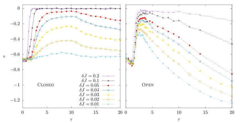
Figure 5: Energy density of driven sites for a closed spin chain (left, $\ell=40$) and an open one (right $\ell=20$, $L=2000$). For the dynamical distributions, due to the symmetric structure of the Hamiltonian, energy density $e=0$ corresponds to the ‘infinite temperature’ ensemble. In both plots, the strength of the disorder $\delta J$ increases from bottom to top, which leads to an increasingly steep rise in energy absorption around $\tau\approx 1$. The initial energy density has been chosen as $e_{\rm initial}=-0.66$, and curves are averages over $\mathcal{N}=8000$ trajectories at $t=1000\tau$.

V.2 Synchronisation

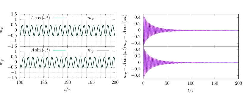
Figure 6: Synchronisation of open system. Left: local magnetisations $m_{x}$ and $m_{y}$, compared with the scaled magnetic field projected onto the corresponding direction, where the scaling factor $A=0.501$ has been fitted. Right: difference between these functions. There is a transient period of approximately 100 cycles, after which the system is well synchronised up to small errors. Here, we have set $\tau=10$, $\ell=40$, $L=2000$, $e_{\rm initial}=-0.66$, $\delta J=10^{-3}$ and simulations are averaged over $\mathcal{N}=800$ trajectories.

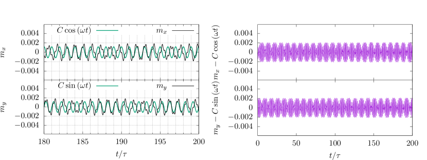
Figure 7: Lack of synchronisation of closed system. Left: local magnetisations $m_{x}$ and $m_{y}$, compared with the scaled magnetic field projected onto the appropriate direction, where the scaling factor $C=-0.00117$ has been fitted. Right: difference between these functions. No synchronisation is observable over any significant timescale. Here, we have set $\tau=10$, $\ell=L=40$, $e_{\rm initial}=-0.66$, $\delta J=10^{-3}$, and simulations are averaged over $\mathcal{N}=4000$ trajectories.

The relationship between heating and synchronisation can be described intuitively by examining the continuous-time dynamics of the driven spin chain. To this end, we first note that the total energy absorption over the time $t$ can be expressed as

$$L\left[\mathfrak{e}(t)-\mathfrak{e}_{\rm initial}\right] =\int_{0}^{t}\mathrm{d}s\left\langle\frac{\mathrm{d}}{\mathrm{d}s}\mathcal{H}(s)\right\rangle_{0}$$ (42)

$$=\ell\int_{0}^{t}\mathrm{d}s\,\dot{\bf B}(s)\cdot\langle{\bf m}\rangle_{0},$$

where $\langle\cdots\rangle_{0}$ denotes the average over initial states, the magnetisation ${\bf m}$ of the system proper is defined according to Eq. (10), and $\mathfrak{e}$ is the energy density of the entire system. Hence, the total energy absorption vanishes if $\langle{\bf m}(s)\rangle_{0}\propto{\bf B}(s)$ for all times. Fig. 7 shows that, after a transient phase of about 100-200 cycles, the open system, indeed enters a state where this synchronisation condition is nearly met and the rate of energy absorption is minimal. We note that the remaining deviations, which cause residual heating in the slow-driving regimes, cannot be explained by a constant phase lag.

By contrast, no synchronisation takes place in the closed system as shown in Fig. 6; instead the deviations from the synchronisation condition are homogeneous on a scale $t\sim 11\tau$. This timescale comes from the beating frequency $\sqrt{1+\omega^{2}}-\omega$ of the exact solution for the closed system magnetisation in the clean limit $\delta J=0$. At the same time, these deviations are of the same order of magnitude as in the synchronised state of the open system, containing a statistical contribution from finite sampling of the initial conditions as well as deviations induced by finite $\delta J$.

To understand these observations, we may again invoke the rotating-frame picture of Sec. IV.2, where the Hamiltonian of the entire system is given by Eq. (37) and the system proper is subject to the effective magnetic field ${\bf B}_{\rm eff}=\hat{\bf x}-\omega\hat{\bf z}$. The magnetisation of the system proper parallel to ${\bf B}_{\rm eff}$ is conserved up to corrections of order $\delta J$, and therefore does not change significantly on relevant time scales. This almost-conservation law is broken once the system proper is coupled to the reservoir. As a result, a persistent magnetisation builds up in the $x$-direction as the entire system relaxes to the effective Gibbs ensemble (31). In the lab frame, this process corresponds to the synchronisation observed in Fig. 7. It thus also becomes clear that the deviations from the synchronisation condition that persist in both the closed and the synchronised open system should be attributed to the disorder in the coupling constants, which renders the rotating-frame Hamiltonian a non-conserved quantity, regardless of the presence of the reservoir. Finally, since the open system is able to redistribute energy into the reservoir, its effective heating rate, incurred by the residual energy absorption due to imperfect synchronisation, is strongly suppressed compared to the closed system.

V.3 Profiles

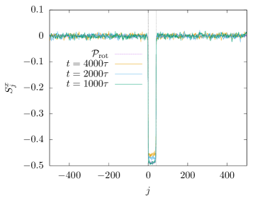
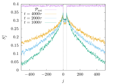
Figure 8: Spatially resolved profiles for $S_{j}^{x}$ and $S_{j}^{z}$ in the slow-driving regime $\tau=10$ for $\ell=40$, $L=2000$, $\delta J=10^{-3}$, $e_{\rm initial}=-0.66$. Shown are the dynamical results, averaged over $\mathcal{N}=8000$ trajectories, for various $t$, compared with the rotating-frame ensemble $\mathcal{P}_{\mathrm{rot}}$ of Eq. (31) averaged over $\mathcal{M}=32000$ MC samples. Boundaries of the system proper are indicated by vertical dashed lines.

Our understanding of the low-frequency regime rests on the assumption that in the rotating frame the system relaxes to the global Gibbs state of Eq. (31) on a timescale that is well separated from the heating timescale determined by $\delta J$. Given the form of the $z$-field present in the Hamiltonian of Eq. (30), one might expect that this relaxation happens uniformly throughout the reservoir. As a matter of causality, however, the reservoir spins far away from the driven sites cannot be instantly affected by the driving. In fact, the interaction strength sets the scale for a finite group velocity $v\sim J=1$, and any correlation function involving solely degrees of freedom separated by a distance $r$ cannot distinguish between the driven and undriven systems outside of the light-cone $r>vt$. Hence, the rearrangement of local degrees of freedom and the large-scale spread of correlations must occur on different timescales.

To uncover the inhomogeneous nature of the relaxation process explicitly, we calculate the spatial profiles of the local observables $S_{j}^{x}$ and $S_{j}^{z}$. These data, plotted in Figs. 1 and 8, show that for low-frequency driving the $x$- and $z$-magnetisations of the system proper have settled to the flat profiles predicted by the local Gibbs state of Eq. (33) after around 1000 cycles. At this time, the $z$-magnetisation profile of the reservoir is neither homogeneous nor stationary.

To understand the mechanism of the subsequent global relaxation process, we may observe that the $z$-magnetisation is a locally conserved quantity everywhere in the bulk of the reservoir, up to corrections of order $\delta J$. The breaking of this conservation law at the boundary of the reservoir, where the system proper generates an oscillating magnetic field perpendicular to $\hat{\bf z}$, leads to gradual build-up of the $z$-magnetisation profile. This profile spreads, presumably diffusively, into the reservoir and eventually becomes flat when the system has fully relaxed to the global Gibbs state of Eq. (31). At the same time, deviations from synchronisation in the system proper cause small heat currents to flow into the reservoir and elevate its overall energy density on the heating timescale set by $\delta J$.

We may now return to the question of how to determine the effective inverse temperature $\beta_{\rm rot}$ for the rotating-frame ensemble encountered in Sec. IV.2. According to statistical mechanics, this parameter should be fixed by energy conservation, as indicated by Eq. (32). However, this approach assumes that the system has fully relaxed to the global Gibbs state (31), which, as shown by Figs. 1 and 8, is clearly not the case for the evolution times considered in Fig. 4. It is therefore surprising that $\beta_{\rm rot}$ as determined by Eq. (32) yields excellent agreement between ensemble and dynamical distributions at very low frequencies short-paper . A posteriori, this result may be attributed to the fact that the virtual magnetic field on the reservoir, and thus the amplitude of the emerging magnetisation profile are small for $\omega\ll 1$. Thus the initial state of the reservoir does not deviate substantially from its rotating-frame Gibbs state. Away from ultra-low frequencies, agreement between ensemble and dynamical distributions may still be achieved by fitting $\beta_{\rm rot}$ to the mean energy of the system proper, as we have shown in Sec. IV.2. This observation suggests that the reservoir locally reaches an effective equilibrium state at its boundary with the system proper on a much smaller timescale than that of the global relaxation process.

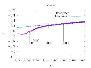
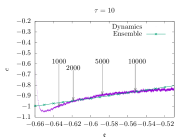
Figure 9: Implicit relationship between the energy density of the total system $\mathfrak{e}$ and the system proper only $e$. The green curve is produced by sweeping $\beta_{\rm rot}$ and evaluating the energy density of both system proper and total system from the ensemble of Eq. (31). The purple data is an average of $\mathcal{N}=8000$ dynamical evolutions with $\ell=40$, $L=4000$, $\delta J=10^{-3}$, $e_{\rm initial}=-0.66$. The number of cycles elapsed are indicated by arrows.

This reasoning implies an implicit relationship between the energy density of the system proper $e$, and that of the entire system $\mathfrak{e}$, which can be probed quantitatively. In the rotating-frame ensemble (31), both $e$ and $\mathfrak{e}$ are determined by a single parameter, $\beta_{\rm rot}$. If we assume that relaxation to this ensemble occurs on a much faster timescale than heating, we may described the system by an effective rotating-frame Gibbs state with inverse temperature $\beta_{\rm rot}=\beta_{\rm rot}(t)$ after some transient period. We may thus sweep $\beta_{\rm rot}$ through a range of values and plot the energy densities $\mathfrak{e}(\beta_{\rm rot})$ against $e(\beta_{\rm rot})$. This plot can then be compared with the actual values of these quantities obtained from dynamical simulations. The results of this analysis are shown in Fig. 9. For $\tau=10$, the dynamical energy densities come fairly close to values predicted by the effective ensemble for simulation times $t\gtrsim 1000\tau$. In this regime, $\beta_{\rm rot}$ can be accurately determined from energy conservation, which yields excellent results as exhibited in Ref. [short-paper, ]. For $\tau=5$, Fig. 9 shows that this approach is viable only for $t\gtrsim 5000\tau$, which explains why $\beta_{\rm rot}$ required fitting in order to achieve agreement between dynamical and ensemble distributions as seen in Fig. 4 where $t=1000\tau$.

V.4 Non-Markovianity

Throughout this paper, we have described the reservoir by explicitly simulating its full microscopic dynamics. We have, however, not yet considered the option of accounting for the reservoir by modifying only the equations of of the system proper, which might drastically reduce the computational cost of numerical simulations. A full analysis of this approach would go beyond the scope of this work. On the basis of our results we can, however, identify some of its immediate limitations.

The simplest way to construct the dissipative dynamics of the system proper would, arguably, be to replace the equations of motion for the edge spins with the Langevin equation Ma-Dudarev-Semenov-Woo ; Brown

$$\frac{\mathrm{d}{\bf S}_{j}}{\mathrm{d}t} =-{\boldsymbol{\Omega}}_{j}\times{\bf S}_{j}-\gamma_{s}{\bf S}_{j}\times\left({\bf S}_{j}\times{\boldsymbol{\Omega}}_{j}\right)$$ (43)

$$+{\bf h}_{j}(t)\times{\bf S}_{j},\qquad j=1,\ell,$$

and for the remaining sites $j=2,\ldots,\ell-1$ the equations of motion Eq. (3) remain unchanged. Here, ${\bf h}_{j}(t)$ represents a delta-correlated noise vector $\langle h_{i,\alpha}(t)h_{j,\beta}(t^{\prime})\rangle=\mu_{s}\delta_{ij}\delta_{\alpha\beta}\delta(t-t^{\prime})$, $\mu_{s}$ is the noise strength, and $\gamma_{s}$ is a damping constant. To mimic a thermal reservoir at inverse temperature $\beta$, these quantities must obey the fluctuation-dissipation relation $2\gamma_{s}=\mu_{s}\beta$. If the effective magnetic field ${\boldsymbol{\Omega}}_{j}$ is time independent, the system proper then relaxes to the Gibbs state (4).

One might now include the driving by adding the on-sit magnetic field ${\bf B}(t)$ to the effective field ${\boldsymbol{\Omega}}_{j}$. However, our results show that this modification would invalidate the basic assumptions underpinning the Langevin equation (43). Specifically, the Markovian limit i.e. delta-correlated noise, is realised only if the reservoir constantly remains in its initial equilibrium state and its correlation functions decay fast on the observational timescale. As seen in Figs. 1 and 8, however, the full dynamical simulation suggests that, even for $L\to\infty$, an ever-growing region of the reservoir departs from its initial state while correlations with the system proper build up continuously. One should therefore not expect a simple Langevin model with additively incorporated driving to reproduce the dynamics of the system proper accurately, as least beyond the limit of ultra-low frequencies, which is characterised by relaxation to an instantaneous Gibbs state.

In fact, our results show that any attempt to describe the system-proper dynamics at intermediate frequencies by means of dissipative equations of motion would have to give up on the assumption of Markovianity. Whether or not it is still possible to derive accurate and tractable non-Markovian time-evolution equations, e.g. by using Nakajima-Zwanzig projection-operator techniques, remains as an important subject for future research Nakajima ; Zwanzig ; Breuer .

VI Perspectives

The central aim of this paper was to shed new light on the physics of classical many-body systems that are subject to periodic driving while being coupled to a large thermal reservoir. To make progress in this direction, we have modelled both the driven system and the reservoir as spin chains with nearest-neighbour interactions and weak disorder. Since the full Hamiltonian dynamics of this setup can be simulated exactly at moderate numerical cost, we were able to avoid the use of dissipative equations of motion that account for the reservoir in a phenomenological or approximate way. While some of our more quantitative results may be contingent on the specific setting we have considered, we expect our main insights to be representative for a broader class of systems.

In particular, a high-frequency regime, where energy absorption is strongly suppressed and the stroboscopic dynamics of the driven system is governed by its averaged Hamiltonian, plus leading corrections obtained from the classical Floquet-Magnus expansion, should generically exist. Our results corroborate the natural expectation that, in this regime, the reservoir acts, up to small perturbations at its boundary with the driven system, as a nearly reversible heat sink balancing residual energy uptake from the drive. Perhaps more surprisingly, we found that this behaviour changes quite abruptly as the driving frequency decreases below some threshold value, which is determined by the typical energy scale of the system and, to a lesser degree, by the strength of the disorder, see Fig. 5. The system then enters a crossover regime, which is characterised by a sharp increase in energy absorption and covers only a small range of frequencies. Understanding the microscopic mechanism of this crossover as well as its putative dependence on the dimensionality of the system, the nature of the drive and the range of interactions, provides an intriguing and presumably challenging subject for future research.

Upon further reducing the driving frequency, the system eventually enters a low-frequency regime, which connects smoothly to the, most likely universal, quasi-static limit, where the driven degrees of freedom are constantly described by an instantaneous equilibrium state. This regime is characterised by rapid synchronisation between the driven system and the applied field and, away from the quasi-static limit, a gradual rearrangement of reservoir degrees of freedom over long distances, which is accompanied by the steady build-up of long-range correlations. Here, we were able to show that this behaviour may in fact extend over a large range of frequencies, which is limited from above only by the crossover to the high-frequency regime. This analysis, however, crucially relies on the existence of a rotating reference frame, where the Hamiltonian of the entire system is nearly time independent, thus providing a stroboscopically conserved quantity. Whether or not almost conserved quantities, which prevent the system from approaching an infinite-temperature state on a practically long time scale exist for more general systems and driving protocols, remains an open question. It is, however, plausible to expect that such quantities may be constructed at least perturbatively from the quasi-static limit, where the instantaneous Hamiltonian serves as an adiabatic invariant. It would then be interesting to explore whether a qualitatively new type of behaviour emerges between the low-frequency regime and the crossover to the high-frequency regime and how it can be characterised.

Finally, our work opens an interesting perspective in the area of open dynamical systems. As we have briefly discussed at the end of Sec. V, the conventional Langevin-approach to classical open-system dynamics is limited by the assumption of a nearly invariant reservoir with fast decaying correlations on the observational time scales. However, for the system we have analysed here, this condition can be met only near the quasi-static limit, and perhaps in the high-frequency regime upon replacing the system Hamiltonian with a suitably truncated Floquet-Magnus Hamiltonian; in the latter case, it may be possible to develop a classical framework similar to the stochastic-wave-function method in Floquet representation, which provides a dynamical description for open quantum systems subject to rapidly oscillating driving fields Breuer-Petruccione . For intermediate frequencies, however, our results strongly suggest that non-Markovian equations of motion will have to be adopted to describe the dynamics of periodically driven open systems, presumably in both the classical and the quantum case. Finding systematic ways to derive and analyse these equations will require further research. Our present work provides both a starting point for such investigations and a valuable benchmark for their results.

Data access statement

The source code used for all simulations, and all data used in figures, is freely available at https://github.com/tveness/spinchain-papers.

References

- (1) G. Floquet, Scientific annals of the École Normale Supérieure 12, 47 (1883).
- (2) T. Kitagawa, T. Oka, A. Brataas, L. Fu, E. Demler, Phys. Rev. B 84, 235108 (2011).
- (3) H. Sambe, Phys. Rev. A 7, 2203 (1973).
- (4) M. Torres and A. Kunold, Phys. Rev. B 71, 115313 (2005).
- (5) M. Bukov, L. D’Alessio, A. Polkovnikov, Adv. Phys. 64, 139 (2015).
- (6) A. Eckardt, Rev. Mod. Phys. 89, 011004 (2017).
- (7) We thank Anatoli Polkovnikov for bringing this argument to our attention.
- (8) V. I Arnold, A. Avez, Ergodic Problems of Classical Mechanics (1968).
- (9) H. W. Broer, B. Krauskopf, AIP Conference Proceedings 548, 31 (2000).
- (10) L. D. Landau, E. M. Lifshitz, Mechanics. Vol. 1 §30, Pergamon Press (1960)
- (11) T. Kinoshita, T. Wenger, D. S. Weiss, Nature 440, 900 (2006).
- (12) V. Khemani, A. Lazarides, R. Moessner, S. L. Sondhi, Phys. Rev. Lett. 116, 250401 (2016).
- (13) C. W. von Keyserlingk, S. L. Sondhi, Phys. Rev. B 93, 245145 (2016).
- (14) A. Chan, A. De Luca, J. T. Chalker, Phys. Rev. X 8, 041019 (2018).
- (15) C. Weitenberg, J. Simonet, Nat. Phys. 17, 1342 (2021).
- (16) M. S. Rudner, N. H. Lindner, Nat. Rev. Phys. 2, 229 (2020).
- (17) P. Ponte, A. Chandran, Z. Papic, D. A. Abanin, Ann. Phys. 353, 196 (2015).
- (18) A. Lazarides, A. Das, R. Moessner, Phys. Rev. E 90, 012110 (2014).
- (19) A. Russomanno, A. Silva, G. E. Santoro, J. Stat. Mech. 2013(09), P09012 (2013).
- (20) T. N. Ikeda, A. Polkovnikov, Phys. Rev. B 104, 134308 (2021).
- (21) A. Haldar, A. Das, J. Phys.: Condens. Matter 34 234001 (2022).
- (22) A. Lazarides, A. Das, and R. Moessner, Phys. Rev. Lett. 112, 150401 (2014).
- (23) D. Abanin, W. De Roeck, W. W. Ho, F. Huveneers, Commun. Math. Phys. 354, 809 (2017).
- (24) D. A. Abanin, W. De Roeck, W. W. Ho, F. Huveneers, Phys. Rev. B 95, 014112 (2017).
- (25) D. A. Abanin, W. De Roeck, F. Huveneers, Phys. Rev. Lett. 115, 256803 (2015).
- (26) T. Mori, T. Kuwahara, K. Saito, Phys. Rev. Lett. 116, 120401 (2016).
- (27) T. Kuwahara, T. Mori, K. Saito, Ann. Phys. 367, 96 (2016).
- (28) W. Hodson, C. Jarzynski, Phys. Rev. Research 3, 013219 (2021).
- (29) O. Howell, P. Weinberg, D. Sels, A. Polkovnikov, M. Bukov, Phys. Rev. Lett. 122, 010602 (2019).
- (30) A. Pizzi, A. Nunnenkamp, J. Knolle, Phys. Rev. Lett. 127, 140602 (2021).
- (31) A. J. McRoberts, T. Bilitewski, M. Haque, R. Moessner, Phys. Rev. B 105, L100403 (2022).
- (32) T. Veness, K. Brandner, Reservoir-induced stabilisation of a periodically driven many-body system (2022).
- (33) F. Jin, T. Neuhaus, K. Michielsen, S. Miyashita, M. A. Novotny, M. I. Katsnelson, H. De Raedt, New J. Phys. 15, 033009 (2013).
- (34) M. Krech, A. Bunker, D. P. Landau, Comput. Phys. Commun. 111, 1 (1998).
- (35) M. E. J. Newman, G. T. Barkema, Monte Carlo methods in statistical physics, Clarendon Press (1999).
- (36) J. D. Parsons, Phys. Rev. B 16, 2311 (1977).
- (37) A. Erdélyi, Asymptotic expansions, No. 3. Courier Corporation (1956).
- (38) S. Blanes, F. Casas, J. A. Oteo, J. Ros, Phys. Rep. 470, 151 (2009).
- (39) C. M. Bender, S. Orszag, Advanced mathematical methods for scientists and engineers I: Asymptotic methods and perturbation theory (Vol. 1), Springer Science & Business Media (1999).
- (40) M. Berry, Asymptotics beyond all orders, Springer, Boston, MA (1991).
- (41) T. Mori, Phys. Rev. B 98, 104303 (2018).
- (42) E. B. Fel’dman, Phys. Lett. A 104 (1984).
- (43) A. Rubio-Abadal, M. Ippoliti, S. Hollerith, D. Wei, J. Rui, S. L. Sondhi, V. Khemani, C. Gross, I. Bloch, Phys. Rev. X 10, 021044 (2020).
- (44) P.-W. Ma, S. L. Dudarev, A. A. Semenov, C. H. Woo, Phys. Rev. E 82, 031111 (2010).
- (45) W. F. Brown, Phys. Rev. 130, 1677 (1963).
- (46) S. Nakajima, Prog. Theor. Phys. 20, 948 (1958).
- (47) R. Zwanzig, J. Chem. Phys. 33, 1338 (1960).
- (48) H.-P. Breuer, F. Petruccione, Theory of Open Quantum Systems, Oxford (2002).
- (49) H.-P. Breuer, F. Petruccione, Phys. Rev. A 55, 3101 (1997).