III Simulations

The various components of the proposed methodology are demonstrated in this section, namely the adaptive uncertainty quantification and the integration of frequency stability constraints with bounded use of the stored energy in the optimal scheduling. To achieve this goal, the case study of a wind-powered offshore platform is presented, where a reference operation time period is considered involving both regions of smooth, low magnitude and sudden, large net load variations. The effectiveness of the proposed methodology is then demonstrated with time domain simulations on the scheduling time scale. The optimization problem is solved with Gurobi 9.1.0 in a 28 physical core multi-node cluster with Intel(R) Xeon(R) CPU E5-2690 v4 @ 2.60 Hz and 25 GB RAM. The solution time of LABEL:eq:optProb_general using the proposed formulation is well below 15 minutes, which is assumed here as the minimum threshold for real-time power system scheduling.

III-A Capabilities of adaptive uncertainty quantification

A representative example of how the adaptive uncertainty quantification framework works is illustrated in fig. 3, where a case of a sudden was selected since these are the most interesting from a power imbalance perspective. The actual load values are presented with the solid black line and the blue cross indicates the time instant at which a probabilistic forecast is issued. From that moment and for a given prediction horizon ($k\in\mathcal{K}$), the expected values of the prediction are plotted in red dashed line along with the prediction intervals around them in green at various quantile levels ($\hat{\alpha}$). Samples generated by the estimated are also plotted as purple dots.

The proposed adaptive uncertainty quantification algorithm generates samples that better describe the size of an . Observe that, as the blue cross moves forward in time, the prediction intervals adapt to capture the irregular event of the sudden load increase. Note also that, at the initial time (fig. 3a), the prediction intervals are narrow and all the sampled values fall close and around the actual load values. From the next moment and later (figs. 3d, 3b, 3c, 3e, 3f and 3g), however, the uncertainty increases and the prediction intervals expand to capture the possibility of an irregular sudden load increase. The deterministic forecast, in contrast, fails to capture the variation adequately, because it is dominated by the inertia of past values, a common drawback of auto-regressive models.

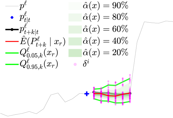
(a) $t+k|t_{0}-3$

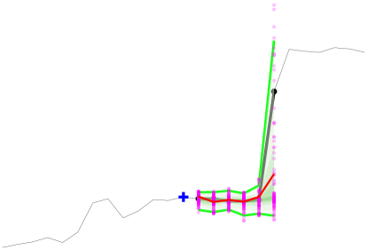
(b) $t_{0}-2$

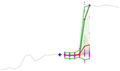
(c) $t_{0}-1$

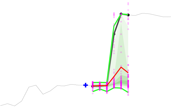
(d) $t_{0}$

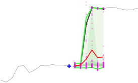
(e) $t_{0}+1$

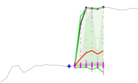
(f) $t_{0}+2$

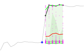
(g) $t_{0}+3$

Figure 3: Demonstration of adaptive uncertainty quantification by using auto-regressive probabilistic forecasting for the load time-series. A case for a sudden step-like variation is presented for consecutive lead times (figs. 3a, 3d, 3b, 3c, 3e, 3f and 3g). By updating the estimated prediction intervals it is possible to capture the sudden load variation and draw samples (purple dots) that span an appropriate range of values.

III-B Effect of optimal and bounded frequency support from ESS

To demonstrate the effect of optimally controlling the to provide frequency support for an isolated , a step is considered at time $t_{0}^{\prime}=2s$ representing a 0.4 pu load increase from a sudden motor startup, where a single is on in the platform of the case study. Simulations were run in Matlab/Simulink 2022a using the model given in LABEL:eq:nlSwing, which do not include delay of actuators. This simplification facilitate the interpretation of results, not implying however any loss of generality.

Results are illustrated in LABEL:fig:stepPlot, where the frequency deviation (solid lines) and the (dashed lines) for two cases are represented. In the first case (grey lines), the single online is the only source of primary frequency control, while, in the second case (black lines), the supports in this task the , which has the same droop setting as in the previous case. Observe that the system’s response in the first case violates not only the steady-state frequency bound $r_{ss}$ but also the maximum allowable ($\bar{\gamma}$), whereas in the second case both limits are respected. To respect the defined bound in the first case, the droop setting must be increased, leading to a larger deviation from the optimal