KDD CUP 2022 Wind Power Forecasting Team 88VIP Solution

Abstract.

KDD CUP 2022 proposes a time-series forecasting task on spatial dynamic wind power dataset, in which the participants are required to predict the future generation given the historical context factors. The evaluation metrics contain RMSE and MAE. This paper describes the solution of Team 88VIP, which mainly comprises two types of models: a gradient boosting decision tree to memorize the basic data patterns and a recurrent neural network to capture the deep and latent probabilistic transitions. Ensembling these models contributes to tackle the fluctuation of wind power, and training submodels targets on the distinguished properties in heterogeneous timescales of forecasting, from minutes to days. In addition, feature engineering, imputation techniques and the design of offline evaluation are also described in details. The proposed solution achieves an overall online score of -45.213 in Phase 3.

1. Introduction

KDD Cup 2022 proposes a dynamic wind power forecasting competition to encourage the development of data mining and machine learning techniques in the energy domain (Zhou et al., 2022). In this challenge, wind power data are sampled every 10 minutes for each of the 134 turbines of a wind farm. Essential features consist of external characteristics (e.g. wind speed) and internal ones (e.g. pitch angle), as well as the relative location of all wind turbines. Given this dataset, we aim to provide accurate predictions for the future wind generation of each turbine on various timescales.

In this paper, we present the solution of Team 88VIP. In general, we ensemble two types of models: a gradient boosting decision tree to memorize basic data patterns (Friedman, 2001; Ke et al., 2017), and a recurrent neural network to capture deep and latent probabilistic transitions (Mikolov et al., 2010; Chung et al., 2014a). Ensemble learning of these two types of models, which characterize different aspects of sequential fluctuation, contributes to improved robustness and better predictive performance (Dong et al., 2020).

Specifically, compared to general time-series forecasting tasks, distinguished properties of wind power forecasting are observed: i) Spatial dynamics: Predictions for each of the 134 turbines are required. The distributions of two turbines are not fully matched, but share a certain spatial correlation (Damousis et al., 2004). ii) Timescales variation: 288-length predictions are required ahead of 48 hours, which cover both the short-term and long-term prediction scenarios (Wang et al., 2021). iii) Concept drift: Due to the large time gap between the test set and the training set, the distribution discrepancy cannot be ignored (Lu et al., 2019).

To tackle these specific challenges, corresponding model components are included. First, the spatial distribution of the turbines is considered for clustering data and imputing missing values. Secondly, submodels training and continual training are proposed to handle the heterogeneous timescales, for tree-based and neural network-based methods, respectively. Third, the distribution drift is adjusted during the inference stage, by comparing the expectation of the predicted values and the average of the ground truth. Empirical results demonstrate the effectiveness of the proposed solution. In all, the proposed solution achieves an overall online score of -45.214 in Phase 3.

2. Method

2.1. Solution overview

In this section, we introduce the total pipeline of the proposed solution, as illustrated in Figure 1. Four essential stages are involved, including: turbine clustering, data preprocessing, model training, and post-processing. And two major models are included through ensemble learning: Gate Recurrent Unit (GRU) and Gradient Boosting Decision Tree (GBDT).

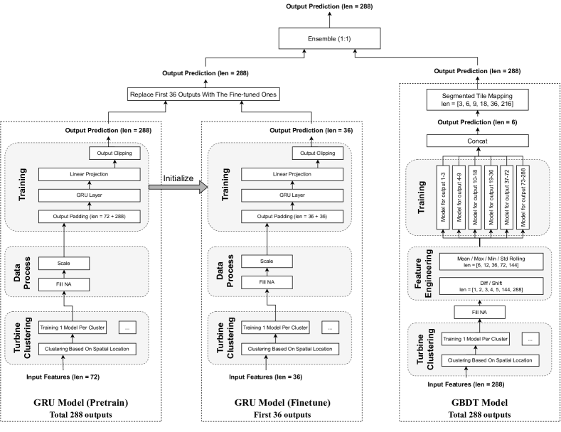
Figure 1. Total pipeline of the proposed solution.

2.2. Solution details

2.2.1. Major models

Gate Recurrent Unit

GRU is a type of recurrent neural network with a gating mechanism (Cho et al., 2014). In recent years, it has shown good performance in many sequential tasks, including signal processing and natural language processing (Su and Kuo, 2019; Athiwaratkun and Stokes, 2017). Through less active in the energy domain, there are studies shows that GRU is well-performed in smaller-sample datasets, compared to other variants of recurrent network (Chung et al., 2014b; Gruber and Jockisch, 2020). For formally, at time $t$, given an element $x_{t}$ in the input sequence, GRU layer updates the hidden state from $h_{t-1}$ to $h_{t}$ as follows:

$$\begin{split}r_{t}=&\sigma\left(W_{ir}x_{t}+b_{ir}+W_{hr}h_{(t-1)}+b_{hr}\right)\,,\\ z_{t}=&\sigma\left(W_{iz}x_{t}+b_{iz}+W_{hz}h_{(t-1)}+b_{hz}\right)\,,\\ n_{t}=&\tanh\left(W_{in}x_{t}+b_{in}+r_{t}\circ\left(W_{hn}h_{(t-1)}+b_{hn}\right)\right)\,,\\ h_{t}=&\left(1-z_{t}\right)\circ n_{t}+z_{t}\circ h_{(t-1)}\,,\end{split}$$

where $r_{t}$, $z_{t}$, and $n_{t}$ represent the reset, update and new gates, respectively; $\sigma$ is the sigmoid function and $\circ$ denote the Hadamard product.

Gradient boosting decision tree

GBDT is an ensemble of weak learners, i.e., decision trees (Hastie et al., 2009). Iteratively, boosting helps to increase the accuracy of the tree-based learner, to form a stronger model (Mason et al., 1999). In addition, both model performance and interpretability can be achieved (Wu et al., 2008).

2.2.2. Main stages

Turbine clustering

As demonstrated in Figure 1, the first stage is clustering the 134 turbines. Data in each cluster can then be processed and trained individually to improve the efficiency and effectiveness of training. In terms of clustering method, neighbored turbines can be placed into the same cluster according to relative location. Alternatively, statistical correlation of wind power series can be also used. Empirically, we find that spatial clustering outperforms that relying on correlation, as further detailed in Section 3.4.1.

Data preprocessing

In the second stage, we preprocess the dataset. To deal with the large amount of missing values and abnormal values, data imputation techniques are employed, either by the average within the cluster, or by a linear interpolation based on time series. For GRU, data scaler is applied on numeric features. Details are provided in Section 3.1. For GBDT, feature engineering is performed to reconstruct the features used in the model training, including: the mean, max, min and standard deviation with the rolling in the historical sequences. More precisely, we consider that the lengths of the rolling window range from 6 to 144, i.e., from one hour to one day. In addition, values differences between the last timestamps and the history, ranging from last 10 minutes to two days, are also taken into account.

Model training

GRU and GBDT are trained individually for each turbine cluster. For both, the mean square error (MSE) is considered as the training loss.

To deal with the heterogeneous timescales in the 288-length outputs, we separately develop training techniques for the two models. For GRU, we first pretrain the model with input length (=72) and output length (=288) for multiple epochs (=20); after that, we finetune the solution with a relatively small input length (=36) and output length (=36), such that the finetuned solution focuses more on the short-term prediction. Finally, we replace the first 36 points in the pretrained outputs with the finetuned ones, to obtain the final prediction. And for GBDT, different submodels are trained for different timescales of outputs. In this way, each submodel can extract the important features separately for short-term prediction and long-term prediction. Detailed empirical studies are described in Section 3.4.2.

Post-processing

During inference, regular post-processing consists of clipping the predicted output to a reasonable range and smoothing the prediction curve to a certain level. Specifically, due to the large time gap between the test set and training set, the distribution discrepancy can not be ignored, especially in the online prediction task. In this case, adjusting the prediction results to the average of the ground truth contributes to an improvement of global predictive performance. A simple yet efficient way is to multiply each predicted value by a constant $\alpha>0$. Intuitively, if the average of all ground truth is greater than the average of all predictions, then the optimal $\alpha$ > 1; otherwise, $\alpha$ < 1. More formally,

$$\alpha=\arg\min\ell(\hat{y},y;\alpha)=\sum_{i}{(\alpha\hat{y}_{i}-y_{i})^{2}}+\sum_{i}{|\alpha\hat{y}_{i}-y_{i}|}\,,$$

where $\hat{y}$ denotes the predicted values and $y$ the ground truth. The existence of an optimal solution is guaranteed considering that the loss function $\ell$ is convex w.r.t. $\alpha$. Empirical experiments related to the adjustment parameters are described in Section 3.4.3.

3. Experiments

We conduct comprehensive experiments to demonstrate the effectiveness of our solution. In this section, we focus on i) providing an overall predictive performance of both online and offline datasets; ii) providing detailed ablation study to analyze the effectiveness of modules, mainly in an offline setting.

3.1. Data preprocessing

Firstly, we introduce how the official training and test data are preprocessed.

Invalid cases imputation

We encode the invalid conditions, including both the abnormal values and missing values, as “NA” (not available). Abnormal values include cases where the wind power is negative or equals zero while the wind speed is large (Zhou et al., 2022). As summarized in Table 1, the invalid conditions account for about a third of the total samples. To handle these values, we perform a two-step imputation strategy to reduce uncertainty and bias in the prediction (Rubin, 1988; Schafer, 1999). Firstly, we substitute the missing values with the average within the cluster; Secondly, for those not sharing any valid conditions within the cluster, we perform a linear interpolation based on time-series.

Table 1. Dataset statistics.

	# day	# samples	# abnormal	# missing
Training	245	4 727 520	1 354 025	49 518
Test	16	308 736	104 625	2 663

Data scaling

Following data imputation, we apply the feature scaler to keep the relative scales of features comparable. Considering that data have outliers as illustrated in Figure 2, a robust scaler is applied, which removes the median and scales the data according to the range between the $1^{\text{st}}$ quartile and the $3^{\text{rd}}$ quartile (Pedregosa et al., 2011). More formally, for each column $x$:

$$x_{\text{scaled}}=\frac{x-x_{\text{median}}}{x_{q75}-x_{q25}}\,.$$

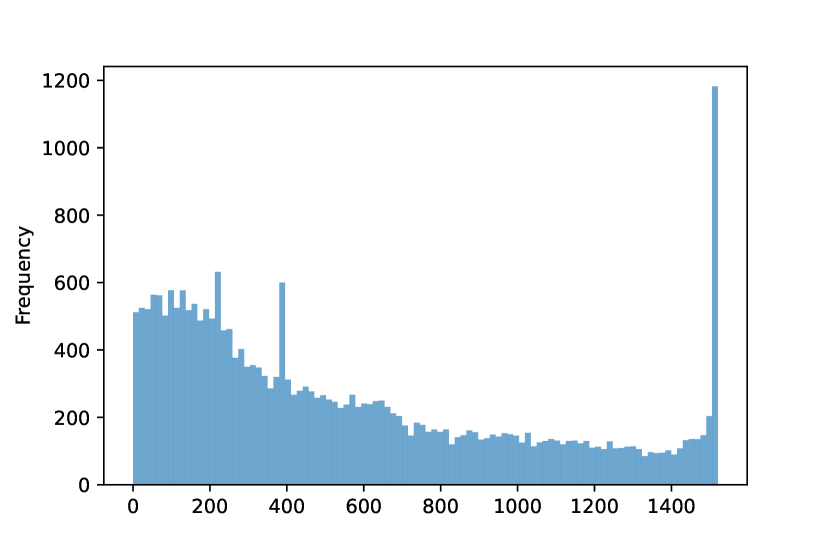
(a) Wind power.

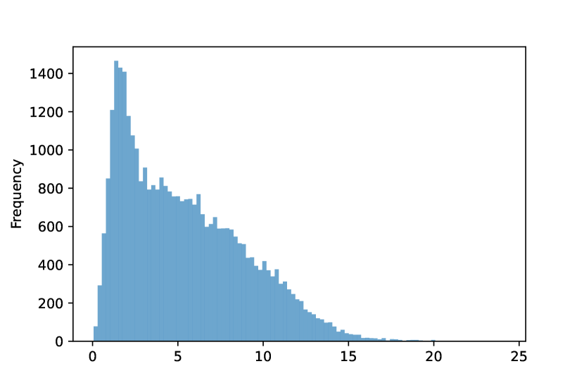
(b) Wind speed.

Figure 2. Visualizing data distribution. (a) Wind power. (b) Wind speed. Values less than 0 are removed in the plots.

Test set reconstruction

The official test set defines a 2-day ahead forecasting evaluation given 14-day historical sequence. However, a single evaluation of one 288-length output is far from reliability. In addition, in our solution, the maximum input length is set as 288 (2 days). Thus we can reconstruct the test set, by randomly splitting the total 16 days to turn a single evaluation into 30 times through rolling windows. In this way, multiple evaluations guarantee the reliability of the offline results.

Table 2. Online and offline forecasting performance of GBDT, GRU and the final ensemble models. The execution time is also provided. Improv row shows the absolute improvements of the ensemble model over the best-performed single contributing model.

	Online		Offline						Time
	Phase 3	Phase2	Overall Score	RMSE	MAE	6Hours Score	Day1 Score	Day2 Score	Train	Eval
GBDT	-	-44.430	-49.788	53.977	45.600	-32.537	-46.526	-53.032	40 min	25 min
GRU	-	-44.370	-49.797	53.924	45.670	-32.946	-46.434	-53.051	100 min	10 min
Ensemble	-45.213	-44.195	-49.646	53.775	45.517	-32.406	-46.302	-52.935	-	35 min
Improv	-	+0.175	+0.142	+0.149	+0.083	+0.131	+0.132	+0.097	-	-

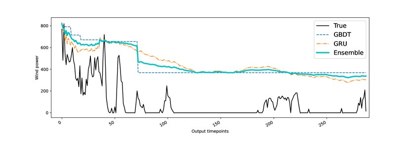
Figure 3. An extract of 288-length prediction results.

3.2. Hyperparameter setting

The hyperparameters for GRU are as listed in Table 3. Adam is applied for model optimization (Kingma and Ba, 2015). For GBDT, we choose the first 200 days to train the model, while the remaining 45 days are used for hyperparameter tuning and early stopping. The maximum number of boost rounds is set as 1000 and the early stopping step is 20. Specifically, the other essential hyperparameters, including the number of leaves, the learning rate and the bagging parameters, are individually tuned for each submodel. Please refer to the codes for their precise values.

We conduct all the experiments on a machine equipped with a CPU: Intel(R) Xeon(R) Platinum 8163 CPU @ 2.50GHz, and a GPU: Nvidia Tesla v100 GPU.

Table 3. Main hyperparameter settings for GRU.

Hyperparameter Names	Values
GRU layers	2
GRU hidden units	48
Numeric embedding dimension	42
Time embedding dimension	6
ID embedding dimension	6
Dropout rate	0.05
Learning rate	$10^{-4}$

3.3. Overall performance

Table 2 illustrates the overall performance of the investigated solution. The improvement of ensemble model over the best-performed single contributing model is also reported. For evaluation metrics, apart from RMSE, MAE, and the overall scores of the total 288-length prediction, we also consider the scores of various output timescales, including those of the first 6 hours (6Hours Score), the first day (Day1 Score) and the second day (Day2 Score).

According to Table 2, the overall results are comparable between two single contributing models. However, in the offline setting, we can explore their slight variations among different timescales: On average, GBDT is better-performed in the first 6 hours prediction, while GRU surpasses GBDT in Day 1, which indicates the two models contribute diversely to the prediction. Meanwhile, we can observe consistent improvements of the ensemble model on all metrics from offline to online. For instance, the ensemble model gains 14.20% offline score, and 17.50% online score (Phase 2) over the single contributing models. The improvements come from the reduction of prediction bias and variation by aggregating two type of models with diversity.

For a more intuitive comprehension, a representative example of forecasting results is showed as Figure 3. In addition, offline training and evaluation time are also reported in Table 2.

3.4. Effectiveness of model components

Now we analyze how the various model components impact the forecasting performance.

3.4.1. Ablation study of turbine clustering

One of the most essential model components is clustering turbines to achieve a more effective and efficient training. More precisely, we compare the way of turbine clustering, either according to the spatial relative positions or to the statistical correlation of the wind power time-series. As demonstrated in Figure 6, in practice, 24 clusters based on turbine location result in relatively good performance for GRU. Similarly, 4 clusters according to the turbine location is the best set-up for GBDT.

Figure 4. Number of turbine clusters (spatial positions). Specifically, Number 134 indicates the case of turbine-level individual modelling; Number 1 corresponds to a unified model for all turbines.

Figure 5. Clustering methods.

Figure 6. Effectiveness of turbine clustering (GRU). (a) Comparison of the number of turbine clusters, according to spatial positions. (b) Comparison of clustering methods.

Table 4. Important features for submodels of GBDT.

Submodels	Timescales	Top 3 important features
0 - 3	0-30 min (short-term)	Time
		Patv
		Patv diff
18 - 36	3-6h (mid-term)	Time
		Wspd
		Patv mean rolling 72
72 - 288	12h-2days (long-term)	Wspd max rolling 144
		Wspd std rolling 144
		Patv std rolling 144

3.4.2. Ablation study of heterogeneous timescales training

To deal with heterogeneous timescales in 288-length outputs, we train submodels for GBDT, and perform continual training for GRU, respectively. The effects of training techniques are shown in Figure 9.

More specifically, we investigate the most important features for each GBDT submodel. Table 4 shows that short-term and long-term predictions rely on different genres of features. For example, short-term predictions depend mostly on the latest values in the historical sequences, while long-term predictions focus more on the periodical statistical features such as the average wind power in the past 24 hours.

Figure 7. Number of submodels for GBDT. Number 6 corresponds to six submodels for output timescales $1-3-9-18-36-72-288$. Based on that, number 7 corresponds to splitting the last part to $72-144-288$. And number 2 for two submodels $1-72-288$.

Figure 8. Continual training for GRU.

Figure 9. Effectiveness of training on heterogeneous timescales. (a) Comparison of the number of submodels for GBDT. (b) Effectiveness of continual training for GRU.

3.4.3. Ablation study of the concept drift in prediction

To correct the concept drift in prediction, the ablation study of adjustment parameter $\alpha$ is conducted in Phase 3 online, as shown in Table 5.

Table 5. Effectiveness of adjustment parameter for online inference. Improvement column indicates the absolute improvement w.r.t. the score without adjustment ($\alpha=1$).

Adjustment parameter $\alpha$	Online Score (Phase 3)	Improvement
0.95	45.750	-0.300
1 (no adjustment)	45.450	-
1.05	45.274	+0.176
1.10	45.213	+0.237

Note that the ablation studies in one component have been conducted with all other hyperparameters equal. Through testing all possible combinations offline, consequently, the optimal solution is summarized in Table 2. Finally, for the reproducibility issue, we have repeated multiple times in the offline scenario, and the variation of the evaluation results is strictly controlled under 0.2%.

4. Conclusion

In summary, GBDT memorizes the basic data patterns and GRU captures the deep and latent sequential transitions. Ensemble learning of these two models, which characterize different aspects of sequential fluctuation, leads to enhanced model robustness. The detailed design of each stage, including turbine clustering, data preprocessing, model training, and post processing, simultaneously contribute to a better predictive performance, empirically verified from offline to online.

There are several possible directions to explore in future work. First, more ensemble strategies can be considered, in addition to the average of prediction results. Secondly, farm-level forecasting task instead of the current turbine-level maybe interesting and beneficial in practice. Last but not least, uncertainty forecasting such as quantile regression or other probabilistic models is another center of new energy AI research that worth exploring.

References

- (1)
- Athiwaratkun and Stokes (2017) Ben Athiwaratkun and Jack W Stokes. 2017. Malware classification with LSTM and GRU language models and a character-level CNN. In 2017 IEEE international conference on acoustics, speech and signal processing (ICASSP). IEEE, 2482–2486.
- Cho et al. (2014) Kyunghyun Cho, Bart van Merriënboer, Dzmitry Bahdanau, and Yoshua Bengio. 2014. On the Properties of Neural Machine Translation: Encoder–Decoder Approaches. In Proceedings of SSST-8, Eighth Workshop on Syntax, Semantics and Structure in Statistical Translation. Association for Computational Linguistics, Doha, Qatar, 103–111. https://doi.org/10.3115/v1/W14-4012
- Chung et al. (2014a) Junyoung Chung, Caglar Gulcehre, Kyunghyun Cho, and Yoshua Bengio. 2014a. Empirical evaluation of gated recurrent neural networks on sequence modeling. In NIPS 2014 Workshop on Deep Learning, December 2014.
- Chung et al. (2014b) Junyoung Chung, Caglar Gulcehre, KyungHyun Cho, and Yoshua Bengio. 2014b. Empirical evaluation of gated recurrent neural networks on sequence modeling. arXiv preprint arXiv:1412.3555 (2014).
- Damousis et al. (2004) I.G. Damousis, M.C. Alexiadis, J.B. Theocharis, and P.S. Dokopoulos. 2004. A fuzzy model for wind speed prediction and power generation in wind parks using spatial correlation. IEEE Transactions on Energy Conversion 19, 2 (2004), 352–361. https://doi.org/10.1109/TEC.2003.821865
- Dong et al. (2020) Xibin Dong, Zhiwen Yu, Wenming Cao, Yifan Shi, and Qianli Ma. 2020. A Survey on Ensemble Learning. Front. Comput. Sci. 14, 2 (apr 2020), 241–258. https://doi.org/10.1007/s11704-019-8208-z
- Friedman (2001) Jerome H. Friedman. 2001. Greedy function approximation: A gradient boosting machine. The Annals of Statistics 29, 5 (2001), 1189 – 1232. https://doi.org/10.1214/aos/1013203451
- Gruber and Jockisch (2020) Nicole Gruber and Alfred Jockisch. 2020. Are GRU cells more specific and LSTM cells more sensitive in motive classification of text? Frontiers in artificial intelligence 3 (2020), 40.
- Hastie et al. (2009) Trevor Hastie, Robert Tibshirani, Jerome H Friedman, and Jerome H Friedman. 2009. The elements of statistical learning: data mining, inference, and prediction. Vol. 2. Springer.
- Ke et al. (2017) Guolin Ke, Qi Meng, Thomas Finley, Taifeng Wang, Wei Chen, Weidong Ma, Qiwei Ye, and Tie-Yan Liu. 2017. LightGBM: A Highly Efficient Gradient Boosting Decision Tree. In Advances in Neural Information Processing Systems, I. Guyon, U. Von Luxburg, S. Bengio, H. Wallach, R. Fergus, S. Vishwanathan, and R. Garnett (Eds.), Vol. 30. Curran Associates, Inc. https://proceedings.neurips.cc/paper/2017/file/6449f44a102fde848669bdd9eb6b76fa-Paper.pdf
- Kingma and Ba (2015) Diederik P. Kingma and Jimmy Ba. 2015. Adam: A Method for Stochastic Optimization. In 3rd International Conference on Learning Representations (San Diego, CA, USA) (ICLR ’15). http://arxiv.org/abs/1412.6980
- Lu et al. (2019) Jie Lu, Anjin Liu, Fan Dong, Feng Gu, João Gama, and Guangquan Zhang. 2019. Learning under Concept Drift: A Review. IEEE Transactions on Knowledge and Data Engineering 31, 12 (2019), 2346–2363. https://doi.org/10.1109/TKDE.2018.2876857
- Mason et al. (1999) Llew Mason, Jonathan Baxter, Peter Bartlett, and Marcus Frean. 1999. Boosting algorithms as gradient descent. Advances in neural information processing systems 12 (1999).
- Mikolov et al. (2010) Tomas Mikolov, Martin Karafiát, Lukas Burget, Jan Cernockỳ, and Sanjeev Khudanpur. 2010. Recurrent neural network based language model.. In Interspeech, Vol. 2. Makuhari, 1045–1048.
- Pedregosa et al. (2011) F. Pedregosa, G. Varoquaux, A. Gramfort, V. Michel, B. Thirion, O. Grisel, M. Blondel, P. Prettenhofer, R. Weiss, V. Dubourg, J. Vanderplas, A. Passos, D. Cournapeau, M. Brucher, M. Perrot, and E. Duchesnay. 2011. Scikit-learn: Machine Learning in Python. Journal of Machine Learning Research 12 (2011), 2825–2830.
- Rubin (1988) Donald B Rubin. 1988. An overview of multiple imputation. In Proceedings of the survey research methods section of the American statistical association. Citeseer, 79–84.
- Schafer (1999) Joseph L Schafer. 1999. Multiple imputation: a primer. Statistical methods in medical research 8, 1 (1999), 3–15.
- Su and Kuo (2019) Yuanhang Su and C.-C. Jay Kuo. 2019. On Extended Long Short-Term Memory and Dependent Bidirectional Recurrent Neural Network. Neurocomput. 356, C (sep 2019), 151–161. https://doi.org/10.1016/j.neucom.2019.04.044
- Wang et al. (2021) Yun Wang, Runmin Zou, Fang Liu, Lingjun Zhang, and Qianyi Liu. 2021. A review of wind speed and wind power forecasting with deep neural networks. Applied Energy 304 (2021), 117766. https://doi.org/10.1016/j.apenergy.2021.117766
- Wu et al. (2008) Xindong Wu, Vipin Kumar, J Ross Quinlan, Joydeep Ghosh, Qiang Yang, Hiroshi Motoda, Geoffrey J McLachlan, Angus Ng, Bing Liu, Philip S Yu, et al. 2008. Top 10 algorithms in data mining. Knowledge and information systems 14, 1 (2008), 1–37.
- Zhou et al. (2022) Jingbo Zhou, Xinjiang Lu, Yixiong Xiao, Jiantao Su, Junfu Lyu, Yanjun Ma, and Dejing Dou. 2022. SDWPF: A Dataset for Spatial Dynamic Wind Power Forecasting Challenge at KDD Cup 2022. Techincal Report (2022).