Context-Aware Streaming Perception in Dynamic Environments

Abstract

Efficient vision works maximize accuracy under a latency budget. These works evaluate accuracy offline, one image at a time. However, real-time vision applications like autonomous driving operate in streaming settings, where ground truth changes between inference start and finish. This results in a significant accuracy drop. Therefore, a recent work proposed to maximize accuracy in streaming settings on average. In this paper, we propose to maximize streaming accuracy for every environment context. We posit that scenario difficulty influences the initial (offline) accuracy difference, while obstacle displacement in the scene affects the subsequent accuracy degradation. Our method, Octopus, uses these scenario properties to select configurations that maximize streaming accuracy at test time. Our method improves tracking performance (S-MOTA) by $7.4\%$ over the conventional static approach. Further, performance improvement using our method comes in addition to, and not instead of, advances in offline accuracy.

1 Introduction

Recent works like EfficientDet [31], YOLO [3], and SSD [18] were designed for real-time computer vision applications that require high accuracy in the presence of latency constraints. However, these solutions are evaluated offline, one image at a time, and do not consider the impact of increase in inference latency on the application performance. In real-time systems such as autonomous vehicles, the models are deployed in an online streaming setting where the ground truth changes during inference time as shown in Figure 1(a). To evaluate performance in streaming settings, Li et al. [14] proposed a modified metric that measures the model performance against the ground truth at the end of inference. They evaluated object detection models in a streaming fashion, and found that the average precision of the best performing model drops from 38.0 to 6.2, and picking the model that maximizes streaming average precision reduces the drop to 17.8.

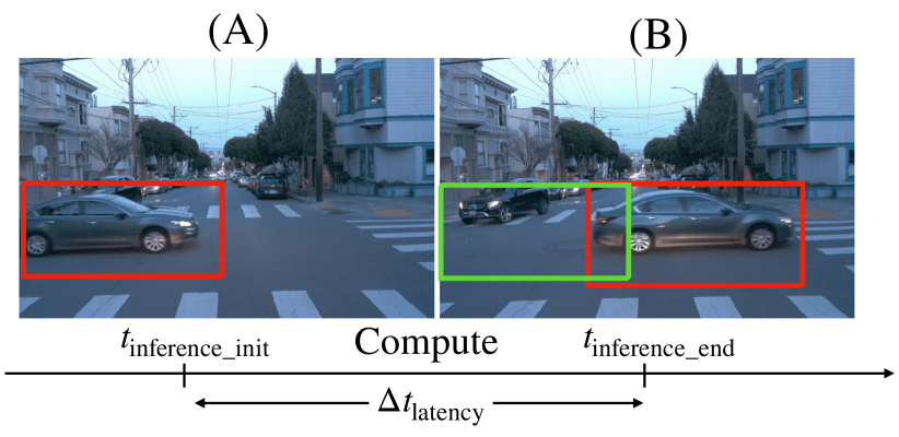
(a) In online streaming settings, the environment changes during inference. Streaming accuracy is computed by evaluating the prediction run on ground truth A against ground truth B.

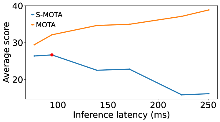
(b) Offline and streaming accuracy of a tracker of increasing model size. While the offline MOTA (orange, y-axis) of the model increases as inference latency (x-axis) increases, its streaming MOTA (S-MOTA in blue, y-axis) decreases.

Figure 1: Streaming accuracy deviates from offline accuracy because the ground truth changes during inference.

We confirm the findings of Li et al. [14], and extend their analysis to object tracking. The standard metric for object tracking is MOTA (multiple object tracking accuracy) [22, 13], and we refer to its streaming counterpart as S-MOTA.  Figure 1(b) shows that larger models with higher MOTA deteriorate in S-MOTA for the Waymo dataset [33] as the higher latency widens the gap between ground truth between inference start and finish. The MOTA of the largest model (EfficientDet-D7x) is 38.9 while the S-MOTA is 16.2. The model that maximizes S-MOTA is EfficientDet-D4 with MOTA of 32.1 and S-MOTA of 26.7.

Since environment context varies, to further analyze the tradeoffs between latency and accuracy, we identify the model that maximizes the S-MOTA of 1-second video segment scenarios in the Waymo dataset. We observe that the best performing model varies widely from scenario to scenario (Figure 2). Scenarios that are difficult (e.g., sun glare, drops on camera and reflection) and still (e.g., standing cars in intersection) show (Figure 2 center) benefit from stronger perception while incurring marginal penalty from the latency increase. On the other hand, simple and fast scenes with rapid movement (e.g., turning, in Figure 2 left), behave the opposite, where performance degrades sharply with latency. As a result, at the video segment-level the optimization landscape of streaming accuracy looks vastly different than on aggregate (Figure 1(b)).

In this paper, we propose leveraging contextual cues to optimize S-MOTA dynamically at test time. The object detection model is just one of several choices that we refer to as metaparameters to consider in an object tracking system. Our method, called Octopus, optimizes S-MOTA at test time by dynamically tuning the metaparameters. Concretely, we train a light-weight second-order model to switch between the metaparameters using a battery of environment features extracted from video segments, like obstacle movement speed, obstacle proximity, and time of day.

Our contributions in this work can be summarized as:

• We are the first to analyze object tracking in a streaming setting. We show that the models that maximize S-MOTA change per scenario and propose that the optimization tradeoffs are a result of scene difficulty as well as obstacle displacement.

• We present a novel method of S-MOTA optimization that leverages contextual features to switch the object tracking configuration at test-time.

• Our policy improves tracking performance (S-MOTA) by $7.4\%$ over a static approach by evaluating it on the Waymo dataset [33]. We improve S-MOTA by $3.4\%$ when we apply this approach on the Argoverse dataset [5].

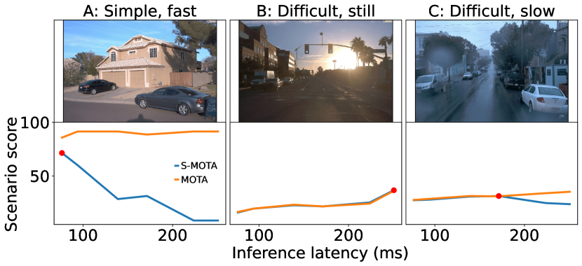
Figure 2: Offline and streaming accuracies in three different scenarios. While offline MOTA (orange, y-axis) of the EfficientDet [31] models increases as inference latency (x-axis) increases, streaming MOTA (S-MOTA in blue, y-axis), responds depending on the scenario context (frames). Compare these plots to Fig. 1(b), which shows the same on average over the entire dataset.

2 Related Works

Latency vs. accuracy. Prior works have recognized the tension between latency and accuracy in perception models [3, 8, 11, 31], and examined facets of the tradeoff between decision speed vs. accuracy [29]. However, these works study this tradeoff in offline static settings. Li et al [14] examine this tradeoff in streaming settings, where the ground truth of the world changes continuously. They show that conventional accuracy misrepresents perception performance in such settings, and proposed streaming accuracy. Their results were shown in detection (as well as semantic segmentation [6]), so we first verified that the idea also holds in tracking. Further, while Li et al. maximize streaming accuracy on average, we expose how the environment context plays a crucial role on its behavior. We leverage the context to dynamically maximize streaming accuracy at test time.

Model serving optimization and dynamic test-time adaptation. To reduce the inference latency, techniques such as model pruning [9, 15, 21] and quantization [28, 34, 37] have been proposed. While these techniques focus on effectively reducing the size of the models, our focus is on the policy: when and where to do it, in order to optimize accuracy in streaming settings. These techniques could be applied to reduce the latency of the models we use. Most similar to our setting are works that leverage context to dynamically adjust model architecture at test time to reduce resource consumption [12, 32] or to improve throughput [30]. This work employs a similar approach in leveraging insight about latency vs. accuracy tradeoff in AV (autonomous vehicle) perception.

Inferring configuration performance without running. Several existing works achieve resource savings by modeling from data how a candidate configuration would perform without actually running it. Hyperstar [23] learns to approximate how a candidate hyperparameter configuration would perform on a dataset without training. Chameleon [12] reduces profiling cost of configurations for surveillance camera detection by assuming temporal locality among profiles. One key differentiating factor with our work is that the prior works were designed for a hybrid setting where some profiling is allowed. In our case, the strict time and compute constraints in the AV setting [16] restrict this approach, requiring an approximation-only method like Octopus.

3 Problem Setup

We first lay out the problem formulation (Sec. 3.1). Next, after an introduction of the Octopus dataset (Sec. 3.2), we measure the accuracy opportunity gap between the global best policy [14] and the optimal dynamic policy (Sec. 3.3). Finally, we perform a breakdown analysis of the components needed in order to optimize streaming accuracy at test time (Sec. 3.4).

3.1 Problem formulation

Given real-time video stream as a series of images, we consider the inference of an AV pipeline (obstacle detection and tracking) on this stream. Let $\mathbb{S}$ denote the mean S-MOTA score of the tracking model, which depends on the values of the metaparameters $\mathcal{H}$, such as object detection model architecture and maximum age of tracked objects. Currently, the metaparameters $h\in\mathcal{H}$ are chosen using offline datasets, and are kept constant during deployment [14]. We refer to this method as the global best approach for statically choosing global metaparameters ($h_{global}$), which are expected to be best across all driving scenarios.

In contrast, in this work we study whether the S-MOTA score $\mathbb{S}$ can be improved by dynamically changing $h$ every $\Delta\tau$ at test time. The metaparameters we choose at each time period $[\tau,\tau+\Delta\tau)$ is $h_{\tau}$, and the corresponding score-optimal values is $h^{*}_{\tau}$.

3.2 The Octopus dataset

To generate the Octopus dataset ($\mathcal{D}$), we divide each video of a driving dataset into consecutive segments of duration $\Delta\tau$. We run the perception pipeline with a range of values of metaparameters $\mathcal{H}$, and record the S-MOTA score for each segment $s^{h}_{\tau}$. We assign the optimal $h^{*}_{\tau}$ to the metaparameters that achieve the highest S-MOTA score (i.e., the optimal S-MOTA score $s^{*}_{\tau}$). The segment duration $\Delta\tau$ is chosen to be short. This allows more accurately studying the performance potential of dynamic streaming accuracy optimization, because decision-making over smaller intervals generally performs better.

We generate the Octopus dataset by recording metaparameter values $h_{\tau}$ and the corresponding S-MOTA scores $s^{h}_{\tau}$ of the Pylot AV pipeline [8] for the Argoverse and Waymo datasets [5, 33]. We execute Pylot’s perception consisting of a suite of 2D object detection models from the EfficientDet model family [31] followed by the Simple, Online, and Real-Time tracker [2]. For each video scenario, we explore the following metaparameters:

• Detection model architecture: selects the model from the EfficientDet family of models, which offers different latency vs. accuracy tradeoff points.

• Tracked obstacles’ maximum age: limits the duration for which the tracker continues modeling the motion of previously-detected obstacles, under the assumption of temporary occlusion or low detection confidence (flickering).

Other metaparameters had limited effect on performance (Appendix 0.A).

We run every metaparameter configuration in a Cartesian product of selected values for each metaparameter, and record latency metrics, detected objects, and tracked objects. The resulting $18$ metaparameter configurations yield $\approx 18,000$ trials. We make this dataset public (https://github.com/EyalSel/Contextual-Streaming-Perception).

Table 1: Dynamically changing metaparameters creates an accuracy opportunity gap. The streaming accuracy (S-MOTA) of the global best metaparameters $h_{global}$ is $6.1$ points lower on average than that of the optimal metaparameters $h^{*}_{\tau}$. Similarly, there is a $3.2$ gap in MOTA (top).

Method	Dataset	MOTA$\uparrow{}$	MOTP$\uparrow{}$	FP$\downarrow{}$	FN$\downarrow{}$	IDsw$\downarrow{}$
Global best	Waymo	37.3	78.1	21515	543193	11615
Optimal	Waymo	40.5	77.6	15738	532678	9137
Global best	Argoverse	63.0	82.1	6721	43376	1284
Optimal	Argoverse	70.8	81.0	5772	34210	828
Method	Dataset	S-MOTA$\uparrow{}$	S-MOTP$\uparrow{}$	S-FP$\downarrow{}$	S-FN$\downarrow{}$	S-IDsw$\downarrow{}$
Global best	Waymo	25.1	72.2	33616	633159	11212
Optimal	Waymo	31.2	71.0	28907	590847	6997
Global best	Argoverse	49.4	75.2	13485	55484	1092
Optimal	Argoverse	57.9	74.1	9562	48354	708

3.3 Accuracy opportunity gap

In order to study if the global best metaparameters $h_{global}$ offer the best accuracy in all driving scenarios, we split the Octopus dataset ($\mathcal{D}$) into train ($\mathcal{D}_{train}$) and test ($\mathcal{D}_{test}$) sets. Next, we compute global best metaparameters ($h_{global}$) as the configuration that yields the highest mean S-MOTA score across all video segments in $\mathcal{D}_{train}$. We denote $h_{global}$’s mean S-MOTA scores on the train and test set as $s^{global}_{train}$ and $s^{global}_{test}$, respectively. Similarly, we denote the mean S-MOTA scores of $h^{*}_{\tau}$ (i.e., optimally changing metaparameters) as $s^{*}_{train}$ and $s^{*}_{test}$.

color=red!40]Ionel: We don’t explain at all why we’ve included MOTA as well.We define the S-MOTA opportunity gap between the optimal dynamic metaparameters and the global best metaparameters as the upper bound of $s^{*}_{test}-s^{global}_{test}$. We repeat the same calculation for MOTA. In Table 1, we show the opportunity gap for the Argoverse and Waymo datasets [5, 33] using $\Delta\tau=1s$. We conclude that optimally choosing the metaparameters at test time offers a $6.1$ (Waymo) and $8.5$ (Argoverse) S-MOTA improvement on average, along with reductions in streaming false positives/negatives and streaming ID switches.

Of note, if offline accuracy were to increase uniformly across all configurations and scenarios, the performance improvement of the dynamic approach over the static baseline is expected to persist. This applies to the opportunity gap shown above (the optimal improvement), as well as for any dynamic policy improvement in this space. This means that performance improvement achieved by dynamic optimization come in addition to, and not instead of, further advances in conventional (offline) tracking. color=gray!40]Eyal: Writing note: Please keep in mind that there are other minor confounding factors beyond non-uniform increase that technically prevent making the last statement outright. The writing is meant to punt these issues to future work

3.4 Streaming accuracy analysis

We approach dynamic configuration optimization as a ranking problem [17], and solve it by learning to predict the difference in score of configuration pairs in a given scenario context [35]. We decompose this learning task into predicting the difference in (i) MOTA, and (ii) accuracy degradation during inference. To our knowledge we’re the first to perform this analysis.

Decomposition. Streaming accuracy (S-MOTA) is tracking accuracy against ground truth at the end of inference, instead of the beginning (MOTA) [14]. Offline accuracy (MOTA) degrades as a result of change in ground truth during inference. The gap between MOTA and S-MOTA is defined here as the “degradation”. Therefore, S-MOTA is expressed as $S-D$ where $S$ is MOTA and $D$ is the degradation. The difference in S-MOTA between two configurations is $(S_{1}-S_{2})-(D_{1}-D_{2})$. This decomposition separates the difference in S-MOTA of two configurations into two parts:

• $(S_{1}-S_{2})$ is the difference in offline accuracy. This difference originates from the MOTA boost, which is affected by (i) the added modeling capacity influenced by the scene difficulty for detection, a specific case of the more general example difficulty [1], and (ii) the max-age choice which depends on the scene obstacle displacement [38].

• $(D_{1}-D_{2})$ is the difference in accuracy degradation. This may be derived from: a. the difference configuration latencies and b. scene obstacle displacement.

Predicting both components to optimize streaming accuracy. At test-time, $S_{1}-S_{2}$ and $D_{1}-D_{2}$ are predicted for each scenario. We find that accurately predicting both components per environment context is necessary to realize the opportunity gap (see Sec. 3.3). First, we show that perfectly predicting $D_{1}-D_{2}$ ($\Delta D^{*}$) and $S_{1}-S_{2}$ ($\Delta S^{*}$) (Table 2, top left) yields $31.2$ S-MOTA, the same as the optimal policy $h_{\tau}^{*}$ on Waymo (Table 1 bottom panel, row 2). Then, we predict $D_{1}-D_{2}$ and $S_{1}-S_{2}$ on average across all scenarios for each configuration ($\overline{\Delta D}$ and $\overline{\Delta S}$ respectively in Table 2). Combining $\overline{\Delta D}$ and $\overline{\Delta S}$ (Table 2, bottom-right) yields $25.1$ S-MOTA, the same as the global best policy $h_{global}$ score on Waymo (Table 1 bottom panel, row 1). The hybrid-optimal policies (Table 2 top-right and bottom-left) achieve $1.8$ ($26.9-25.1$) and $2.7$ ($27.8-25.1$) of the $6.1$ ($31.2-25.1$) optimal policy opportunity gap. Taken together, these results demonstrate the need to accurately predict both the change in MOTA ($S_{1}-S_{2}$) and in degradation ($D_{1}-D_{2}$) per scenario in order to optimize S-MOTA at test time.

	$\Delta D^{*}$	$\overline{\Delta D}$
$\Delta S^{*}$	31.2	26.9
$\overline{\Delta S}$	27.8	25.1

Table 2: Both streaming accuracy components must be predicted per scenario in order to realize the full dynamic policy’s opportunity gap. $\Delta D^{*}$ is optimal degradation prediction, $\Delta S^{*}$ is optimal offline gap prediction. $\overline{\Delta D}$ and $\overline{\Delta S}$ are the corresponding global-static policies.

4 Octopus: Environment-Driven Perception

We propose leveraging properties of the AV environment context (e.g., ego speed, number of agents, time of day) that can be perceived from sensors in order to dynamically change metaparameters at test time. We first formally present our approach for choosing metaparameters, which uses regression to infer a ranking of metaparameter configurations (Sec. 4.1). Then, we describe the environment representation that allows to effectively infer each component of the streaming accuracy (Sec. 4.2).

4.1 Configuration Ranking via Regression

In order to find the metaparameters $h_{\tau}$ that maximize the S-MOTA score $s^{h}_{\tau}$ for each video segment, Octopus first learns a regression model $M$. The model predicts $s^{h}_{\tau}$ given the metaparameters $h_{\tau}$ and the representation of the environment $e_{\tau}$ for the period $\tau$. Following, Octopus considers all metaparameter values, and picks the metaparameters that give the highest predicted S-MOTA.

Executing the model $M$ at the beginning of each segment $\tau$ requires an up-to-date representation of the environment. However, building a representation requires the output of the perception pipeline (e.g., number of obstacles). Octopus could run the current perception configuration in order to update the environment before executing the model $M$, but this approach would greatly increase the response time of the AV. Instead, Octopus makes a Markovian assumption, and inputs the environment representation of the previous segment $e_{\tau-1}$ to the model $M$.

$$M(h_{\tau},e_{\tau-1})=\hat{s}^{h}_{\tau}$$ (1)

Thus, it is important to limit the segment length $\Delta\tau$ as the longer a segment is, the more challenging it is to accurately predict the scores due to using an older environment representation (see Sec. 5.1 for our methodology for choosing $\Delta\tau$).

The model is trained using the mean squared error loss. We choose the metaparameters that the model predicts as the highest score. Let $s^{global}_{\tau}$ denote the S-MOTA score obtained with $h^{global}$ metaparameters, which by definition is a lower bound of the optimal S-MOTA score $s^{*}_{\tau}$ (i.e., $s^{global}_{\tau}\leq s^{*}_{\tau}$). Thus, in order to pick the best metaparameters, Octopus can only predict $s^{h}_{\tau}$ relative to $s^{global}_{\tau}$. As a result, Octopus utilizes the following as the final loss:

$$L=\frac{1}{N}\sum_{i=0}^{N}\left(\hat{r}^{h}_{i}-clip((s^{h}_{i}-s^{global}_{i}),\epsilon)\right)^{2}$$ (2)

color=cyan!40]Justin: is this $\hat{r}^{h}_{i}$ suppose to be the "clipped relative score"where N is the size of the training data and $\hat{r}^{h}_{i}$ is the relative S-MOTA score predicted by the model $M$, $\hat{r}^{h}_{i}=\hat{s}^{h}_{i}-s_{i}^{global}$.

Finally, Octopus clips by lower bounding the predictions by $s^{global}_{i}-\epsilon$ as the predictions significantly below $s_{i}^{global}$ are irrelevant to the optimization problem. Moreover, by clipping the predictions, Octopus reduces the dynamic range of the regressor and makes it easier to predict the higher S-MOTA scores.

4.2 Environment Representation

We can represent the environment context $e_{\tau}$ by capturing the characteristics of the video segment. In order to keep the decision-making latency small, we eschew more complex learned representation designs. Instead, we developed hand-engineered features from sensors and the outputs of the object detection model following prior work by Nishi et al. [24], where the features were used to predict human driving behavior. We collect the features per frame and then aggregate by averaging across frames in the video segment. Unless otherwise specified, we use the 10^th percentile, mean, and 90^th percentile of the following features:

• Bounding box speed is the distance traveled by an object in pixel space across two frames. This feature infers the speed of objects, and thus it is important for capturing obstacle displacement to predict the streaming accuracy degradation.

• Bounding box self IoU is the Intersection-over-Union (IoU) of an object’s bounding box in the current frame relative to the previous frame. color=red!40]Ionel: Is it always the previous frame?Along with the bounding speed, this feature helps isolate the change in size of an obstacle, as it moves towards or away from the ego vehicle. color=red!40]Ionel: How does this feature isolate the change in size? The IoU could also be small if the object moves quickly.

• Number of objects is measured per frame, and indicates the complexity of a scene as the more objects in a scene, the more likely the AV is to encounter object path crossings and occlusions (scene difficulty). Therefore, this feature signals when to prioritize for high offline accuracy configurations that are robust to object occlusions.

• Obstacle longevity is the number of frames for which an obstacle has been tracked. Lower obstacle longevity implies more occlusion as obstacles enter and leave the scene, making perception more difficult. This feature also guides the choice of tracking metaparameters as low obstacle longevities correlate with lower tracking maximum age giving better performance.

• Ego driving speed is the speed at which the AV is traveling, and indicates the environment in which the AV is driving (e.g., highway vs. city).

• Ego turning speed is the angle change of the AV’s direction between consecutive frames. This feature helps differentiate the source of apparent obstacle displacement between obstacle movement and ego movement.

• Time of day hints if a high-accuracy configuration is required to handle challenging scenes (e.g., night driving, sun glare at sunset). color=red!40]Ionel: Nit: might want to specify how it is measured.

We compute these feature statistics for different bounding box size ranges in order to reason about obstacle behavior depending on the detection model strength needed for their accurate detection. For example, higher offline accuracy models do not confer better streaming accuracy if the obstacles in the detectable size range move too rapidly for the longer detection inference time to keep up with.

Note that the choice of metaparameters in each video segment changes the configuration, and hence the outputs of the tracking pipeline. Therefore, the resulting environment representation is no longer independently and identically distributed (i.i.d), making it challenging to use traditional supervision techniques. To keep the data distribution stationary during train time, we use the object detection model as given by the global best metaparameters $h_{global}$. While this training objective is biased considering that the features may be derived from any configuration, we find that it reduces variance during training, and works better than using features derived from the ground truth.

We concatenate the metaparameters $h$ and the environment representation vector $e_{\tau}$, and then use a supervised regression model to predict the score, optimizing using the loss given in Eq. 2.

In addition, we compare our method to a conventional CNN model approach (ignoring its resource and runtime requirements) in Appendix 0.I.

5 Experiments

Next, we analyze our proposed approach. The subsections discuss the following:

• Setup (Sec. 5.1): Description of Datasets and Model Details

• Main results (Sec. 5.2): What is the performance improvement conferred by the dynamic policy over the static baseline?

• Explainability (Sec. 5.3): I. Does the learned policy behavior match human understanding of the driving scenario? II. Where is the learned policy similar to and different from the optimal policy? III. How are scenarios clustered by metaparameter score? IV. What is the relative importance of the hand-picked features and of the metaparameters towards S-MOTA optimization?

• Ablation study (Appendix 0.H): How do various ranking implementation choices affect the final performance?

5.1 Methodology

We evaluate on the Argoverse and Waymo datasets [5, 33], covering a variety of environments, traffic, and weather conditions. We do not use the private Waymo test set as it does not support streaming metrics. However, we treat the Waymo validation set as the test set, and we perform cross validation on the training dataset ($798$ videos for training, and $202$ videos for validation). Similarly, we divide the Argoverse videos into $75$ videos for training, and $24$ for validation. In addition, we follow the methodology from Li et. al [14] in order to create ground truth 2D bounding boxes and tracking IDs, which are not present in the Argoverse dataset. We generate these labels using QDTrack [27] trained on the BDD100k dataset, which is the highest offline accuracy model available.

In our experiments, we run object detectors from the EfficientDet architecture [31] on NVIDIA V100 GPUs, and the SORT tracker [2] on a CPU (simulated evaluation on faster hardware is in Appendix 0.J). We chose to use the EfficientDet models because they are especially optimized for trading off between latency and offline accuracy, and because they are close to the state-of-the-art. The EfficientDet models were further optimized using Tensor RT [25], which both reduces inference latencies to less than $250$ms (the latency of the largest model, EfficientDet-D7x) and decreases resource requirements to at most $3$ GPUs. We use these efficient models to investigate the effect of optimizing two metaparameters: detection model and tracking max age (see Sec. 3.2 for details). We compile $18$ configurations of the AV perception pipeline by exploring the Cartesian product of the values of the two metaparameters (see LABEL:a:config-params).

⬇

1# Metaparameters

2detection-model = {EfficientDet: 3, 4, 5, 6, 7, 7x}

3tracking-maximum-age = {1, 3, 7}

Listing 1: Values for detection and tracking metaparameters.

We implement Octopus’s policy regression model as a Random Forest [4] using Eq. 2 to choose metaparameters for video segment length $\Delta\tau=1s$. We describe training details in Appendix 0.B.

Policy Runtime Overhead. Every step $\Delta\tau$, the Octopus policy applies Random Forest regression for all the $18$ perception pipeline configurations in order to predict the best one to apply in the next step. Due to the lightweight policy design, inference on all $18$ configurations has a latency of at most $6$ms using a single Intel Xeon Platinum 8000 core. As a result, the policy decision finishes before the sensor data of the next segment arrives, and thus does not affect latency of the perception pipeline. Moreover, Octopus pre-loads the perception model weights (13.86GB in total in our experiments) and forward pass activations in the GPU memory ($32$GB), and thus actuates metaparameter changes quickly.

5.2 Main results

We compare the Octopus policy with the optimal policy ($h^{*}_{\tau}$) and the global best policy ($h^{global}$) as proposed by Li et al. [14]. In addition, following the discussion in Sec. 4.2, we show ablations of the Octopus policy in order to highlight the relative contribution in both the setting of predictive and close-loop metaparameter optimization. Concretely, we include the following setups that Octopus can use to optimize the metaparameters at time $t$:

• Ground truth from current segment: features are derived from the sensor data and the labels at time $t$.

• Ground truth from previous segment: features are derived from the sensor data and the labels at time $t-\Delta\tau$.

• Closed-loop prediction from previous segment: features are derived from the sensor data and the output of the perception pipeline for the previous segment (i.e., at time $t-\Delta\tau$).

In Table 3(b) we show the tracking accuracy results for the Waymo and Argoverse datasets. The results show that the Octopus policy with closed-loop prediction outperforms the global best policy by $1.9$ S-MOTA (Waymo) and $1.7$ S-MOTA (Argoverse). Both the optimal and Octopus policies achieve further accuracy increases using features derived from the current segment, further illustrating how rapidly configuration score changes over time. The consistent accuracy improvements across the two datasets show that leveraging environment context to dynamically optimize streaming accuracy provides substantial improvements over the state-of-the-art. Moreover, as discussed in Sec. 3.3, streaming accuracy improvement over the global best policy will likely persist independently of innovation in offline accuracy of the underlying perception models.

Table 3: Streaming tracking accuracy results on two datasets.

(a) Waymo

Method	S-MOTA$\uparrow{}$	S-MOTP$\uparrow{}$	S-FP$\downarrow{}$	S-FN$\downarrow{}$	S-IDsw$\downarrow{}$
Global best	25.1	72.2	33616	633159	11212
Optimal	31.2	71.0	28907	590847	6997
Optimal from the prev. segment	27.2	71.2	38631	603777	8092
Octopus with:
Ground truth from current segment	27.9	72.3	31489	608870	8966
Ground truth from prev. segment	27.3	72.7	31056	612862	9103
Prediction from prev. segment	27.0	72.8	30272	615780	9511

(b) Argoverse

Method	S-MOTA$\uparrow{}$	S-MOTP$\uparrow{}$	S-FP$\downarrow{}$	S-FN$\downarrow{}$	S-IDsw$\downarrow{}$
Global best	49.4	75.2	13485	55484	1092
Optimal	57.9	74.1	9562	48354	708
Optimal from the prev. segment	51.9	74.0	12652	52804	810
Octopus with:
Ground truth from current segment	53.2	74.9	11447	52638	917
Ground truth from prev. segment	51.6	75.1	11348	54502	1010
Prediction from prev. segment	51.1	74.9	12062	54469	1008

S-MOTA vs. S-MOTP. color=cyan!40]Justin: this is way to long; we should instead get to our point. 1. S-MOTA is the metric we chose to optimize. 2. S-MOTP is naturally goes down when S-MOTA goes up (technically not true, cause you can have a better model due to better training data/augmentation). 3. You could optimize S-MOTP if you wanted, look at the supplement.Table 3(b) highlights that both Octopus and optimal policy occasionally deteriorate S-MOTP, inversely to the improvement in S-MOTA. This result reflects on a broader pattern where in streaming settings bounding boxes in general lag after the ground truth, even if by a small enough margin to be counted as true positives. S-MOTP, which is weighted by the IOU between correct predictions and the ground truth is especially hurt as a result. S-MOTA, which just counts the number of false positives, is less affected by this. We provide a longer analysis of this tradeoff/pareto-frontier between S-MOTA and S-MOTP in Appendix 0.D.

5.3 Explainability

We survey various aspects of the metaparameter optimization problem, and qualitatively compare the global best (baseline), the optimal, and the Octopus (learned) policies.

I. Case study: Busy Intersection. Figure 3 shows a scenario where the ego vehicle enters a busy intersection. The scenario is divided into three phases, where the learned (Octopus) policy adaptively tunes the metaparameter to varying road conditions similarly to the optimal policy plan. First, the ego vehicle approaches the intersection with oncoming traffic on the left. The vehicles in the distance cannot be picked up by any of the candidate models. The learned policy chooses D4, the same model as the global best policy. Then, as the light turns yellow and the ego vehicle comes to a stop first in the queue, the learned policy adapts by increasing the strength of the model to D7x. The perception pipeline is now able to detect the smaller vehicles in the opposing lane and adjacent to the road. The optimal policy makes a similar decision while the global best policy remains with the D4 choice, incurring a net performance loss. Finally, as vehicles in the cross-traffic start passing and occluding the vehicles in the background, the learned policy returns to the lower latency D3 model. This scenario illustrates how the learned policy can select the best model in each phase of the scenario, adapting to the change in driving environment.

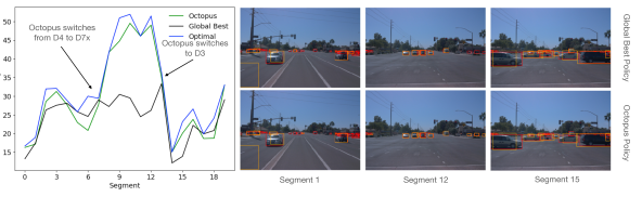
Figure 3: Busy Intersection Scenario. Left: The S-MOTA score of each $\tau=1s$ segment for the Octopus (learned), global best, and optimal policies. Right: The front-facing camera feed. Red bounding-boxes represent the ground truth, and orange represent the pipeline’s predictions using the policy’s configuration choice.

II. Policy action heatmap. In Figure 4, we visualize the learned policy in comparison to the optimal policy. As we expect, the learned policy often selects the global best configuration (D4-1), but expands out similarly to the optimal policy when performance can be improved by changing configurations. This result illustrates how, contrary to common belief that onboard perception must have low latency (e.g. under 100ms [33]), higher perception latencies are tolerable and even preferable in certain environments. The Octopus policy learns to take advantage of this when it opts for higher offline accuracy models. color=gray!40]Eyal: TODO how do we explain the deviations from the optimal policy? Ablating delta S with delta d hat on the t-SNE could reveal some aspectscolor=cyan!40]Justin: Honestly, not necessary; put this in the appendix if you must.

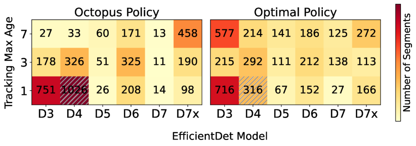
Figure 4: Policy decision frequency. The configuration choice frequency (color intensity) of the Octopus policy (left) and of the optimal policy (right). The global best configuration is EfficientDet-D4 with tracking max age of 1, emphasized with gray stripes.

III. Scenarios are clustered by metaparameter score.

Here, we evaluate whether scenarios are grouped by common metaparameter score behaviors. To this end, we first visualize the scenario score space (explained below) as a t-SNE plot and then perform more formal centroid analysis.

To this end, each video segment of length $\Delta\tau=1s$ is vectorized by computing the MOTA score difference ($S_{c}-S_{h_{global}}$) and degradation difference ($D_{c}-D_{h_{global}}$) for every metaparameter configuration $c$ and the global best configuration $h_{global}$ (see Sec. 3.4). These values are then concatenated and normalized (z-score) across each scenario.

Cluster visualization. We visualize this space in a t-SNE plot in Figure 5. The scenario segment points are colored according to the model that optimizes MOTA (left) and S-MOTA (right). We observe a non-uniform impact of accuracy degradation on the optimal model choice in different video segment regions. This varying effect illustrates that S-MOTA deviates from MOTA setting on an environment context-dependent basis. For case-study analysis of points in the t-SNE please see Appendix 0.F.

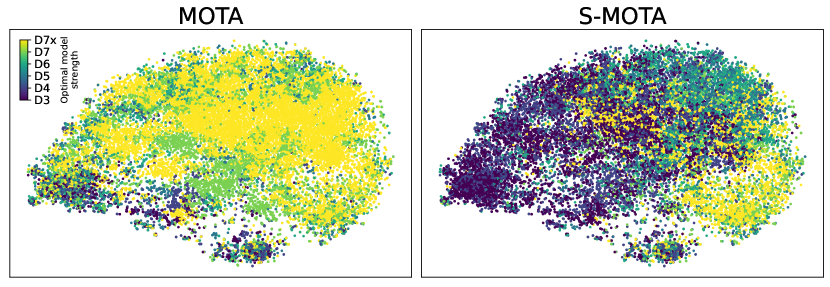
Figure 5: The impact of the accuracy degradation incurred in online streaming context is scenario dependent. Each point is a 1s driving scenario. Its color is the model that maximizes offline accuracy (left) and streaming accuracy (right).

Centroid analysis. We now perform a more formal clustering analysis that reveals modes of metaparameter optimality.

We perform K-means clustering, with k=8 on the z-score space. Figure 6 shows centroids of three representative scenario clusters (right to left): (i) scenarios that benefit from lower latency detection. (ii) scenarios that benefit from higher accuracy detection, and (iii) scenarios that primarily benefit from a lower tracking max age, and to a lesser extent from lower latency detection. These distinct modes reflect that scenarios are grouped around similar metaparameter behaviors, corroborating with variation in scene difficulty and obstacle displacement. The rest of the scenario cluster visualizations are in Appendix 0.G. color=cyan!40]Justin: State the conclusion you want to draw; remove half the details. I assume you want to say: "Intuitively, scenarios with similar preferences for models and max ages are clustered together…" Not sure why I care about this as a reader.

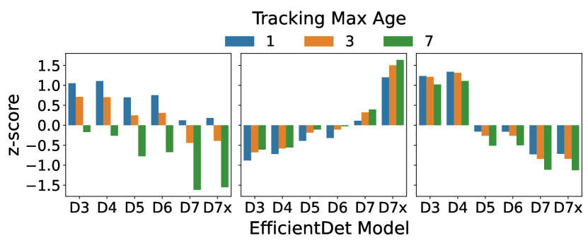
Figure 6: Three centroids of the configuration score distribution: (i) preference for low max age (left), (ii) preference for offline accuracy (middle), and (iii) preference for low latency (right). The three clusters account for 34% of the dataset.

Table 4: Importance study

(a) Feature importance (Regression)

Feature	Importance Score	Feature	Importance Score
Mean BBox self IOU	0.304	BBox bin [665, 1024)	0.087
Mean BBox Speed	0.200	BBox bin [1024, 1480)	0.071
Num. BBoxes	0.063	BBox bin [1480, 2000)	0.055
BBox Longevity	0.076	BBox bin [2000, 2565)	0.040
Ego movement	0.096	BBox bin [2565, $\infty$)	0.417
Time of Day	0.008

(b) Metaparameter importance (Regression)

Metaparameter	S-MOTA$\uparrow{}$	S-MOTP$\uparrow{}$	S-FP$\downarrow{}$	S-FN$\downarrow{}$	S-IDsw$\downarrow{}$
Global best	25.1	72.2	33616	633159	11212
Detection-model	27.6	72.4	26116	615771	11254
Tracking-max-age	25.6	71.9	39400	625184	8973
Both	27.9	72.3	31489	608870	8966

IV. Feature and configuration metaparameter importance.

Feature importance. To study the relative importance of the environment features used in our solution (described in Sec. 4.2), we show the feature importance scores derived from the trained Random Forest regressor in 4(a). The mean bounding box self-IOU and speed together constitute over half of the normalized importance score, as they are predictive of the accuracy degradation that higher-latency detection models would incur. Aggregate bounding box statistics that capture scene difficulty, such as the average number and longevity of the bounding boxes per frame, are also useful for prediction.

Configuration metaparameter importance. In 4(b), we evaluate the gains attributed to each metaparameter by only optimizing one metaparameter at a time, fixing the other parameter to the value in the global best configuration. We do this to ablate the performance shown in Table 3(b), where they are optimized together. In both cases, the models were trained on the ground truth and the present. Although the detection model choice is the primary contributor, the additional choice of occlusion tolerance (max age) further contributes to the achieved performance. We also observe how the performance gain when optimizing the tracker’s maximum occlusion tolerance (see Sec. 3 for details) does not combine additively with the improvement in the detection model optimization.

6 Conclusions

Streaming accuracy is a much more accurate representation of tracking for real-time vision systems because it uses ground truth at the end of inference to measure performance. In this study we show the varying impact that environment context has on the deviation of streaming accuracy from offline accuracy. We propose a new method, Octopus, to leverage environment context to maximize streaming accuracy at test time. Further, we decompose streaming accuracy into two components: difference in offline accuracy MOTA and the degradation, and show that both must be inferred in every scenario to achieve optimal performance. Octopus improves streaming accuracy over the global best policy in multiple autonomous vehicle datasets.

Acknowledgements. We thank Daniel Rothchild and Horia Mania for helpful discussions.

Supplementary Material: Table of contents

• Metaparameter choice (Appendix 0.A)

• Training details (Appendix 0.B)

• Training hyperparameters (Appendix 0.C)

• S-MOTA vs S-MOTP (Appendix 0.D)

• Study-case video (Appendix 0.E)

• t-SNE visualization (Appendix 0.F)

• Full Centroid Visualization (Appendix 0.G)

• Ranking Implementation Ablations (Appendix 0.H)

• Policy Design Using Neural Networks (Appendix 0.I)

• Faster hardware simulation (Appendix 0.J)

Appendix 0.A Metaparameter choice

In this study we use two metaparameters (detection model and tracking maximum age) out of several that we considered initially. These two metaparameters were chosen because (i) they represent 83% of the opportunity gap conferred by all the metaparameters considered together (see below) and (ii) a limited number of metaparameters allows computing the Octopus dataset on more scenarios.

I. Metaparameters we did not use:

• Detection confidence threshold: sets the minimum confidence score of bounding-box predictions to be used by the tracker.

• Minimum matching tracker IOU: sets the minimum bounding-box IOU (Intersection-Over-Union) that the SORT tracker [2] requires to perform obstacle association across frames.

• Tracking re-initialization frequency: specifies every how many frames detection is run to update the tracker. When detection is not run, the SORT tracker falls back on a Kalman filter to linearly extrapolate existing bounding box movement. This option bypasses the detection inference latency, but quickly incurs significant error.

The additional metaparameter ranges are:

⬇

1# Additional Metaparameters

2detection-confidence = {0.4, 0.6, 0.7}

3minimum-matching-tracker-IOU = {0.1, 0.2, 0.3}

4Tracker-re-initialization-frequency = {1, 2, 3}

Listing 2: Values for the other metaparameters.

II. The relative contribution of the two metaparameters we use. The new metaparameter cartesian product (LABEL:a:config-params-full-small) is of size $6*3*3*3*3=486$ configurations. Due to computational constraints, we create a version of the Octopus dataset using 49 training and 23 test scenarios from the Waymo dataset, with $\tau=1s$.

Table 5: Metaparameter contribution to the opportunity gap. The top row shows the score of the global-best policy where no metaparameter changes. Each row below shows the score of the optimal dynamic policy as one additional metaparameter is allowed to change. The incremental score increase is shown on the right.

Dynamic metaparameters	S-MOTA score	Score increase
None (global best policy)	24.0	-
+Detection Model	28.3	4.3
+Tracking maximum age	30.1	1.8
+Tracking re-init frequency	30.5	0.4
+Tracking minimum IOU	31.0	0.5
+Detection confidence threshold	31.3	0.3

Table 5 shows the relative contribution of each metaparameter to the score opportunity gap (Sec. 3.3) between the baseline global best policy and the optimal dynamic policy. The first two metaparameters (detection model and tracking maximum age) are used in our study and achieve $83\%$ ($(30.1-24.0)/(31.3-24.0)$) of the opportunity gap conferred by using all 5 metaparameters. We leave investigation into optimizing the rest of the metaparameters for future work.

Appendix 0.B Training details

During training, we exclude video segments with no ground truth labels, where the MOTA score [22] is undefined. Then, at test time, we impute the global static configuration computed over the training dataset. We clip the regression targets to [-100, 100] (i.e., $\epsilon=100$ in Eq. 2). In our evaluation setup we consider an IOU of 0.4 between a prediction and ground truth to be a true positive. We train the models and evaluate using this schema. We use a single GPU (instead of 3 used in Waymo) for evaluation on the Argoverse dataset, because the high framerate would require over 7 GPUs to support executing detection in parallel on every frame.

Appendix 0.C Training hyperparameters

The training hyperparameters used in training the regression and classification models are shown in Table 6.

Table 6: Training Hyperparameters.

Method	Max Tree Depth	Max # of Features	# of Estimators	Min Impurity Decrease
Regression	20	18	400	0.000186
Classification (Joint)	8	3	400	0.000285
Classification (Independent)	7	4	200	0.000529

The rest of the hyperparameters are the default used in Scikit-Learn v0.23.2.

Appendix 0.D S-MOTA vs S-MOTP

In this work, we demonstrate that environment context can be leveraged to perform test-time optimization of tracking in streaming settings. Unlike other perception tasks (e.g. detection [26]), where a single optimization metric is commonly used, in multi-object tracking there is no consensus on the best metric [7, 20]. Therefore, in this study we chose to optimize MOTA [22], as it is the metric that most closely aligns with human perception of tracking quality [13].

Nevertheless, a battery of other tracking metrics is presented in the evaluation Sec. 5.2. The main results (Table 3(b)) show that the S-MOTA-optimal policy deteriorates in S-MOTP, and that our learned policy does the same in the Argoverse dataset. This occurs because MOTA and MOTP are designed to describe fundamentally different properties in tracking [22]: Whereas MOTA equally balances precision, recall and identification, MOTP only focuses on precise obstacle localization. Indeed, Table 7 empirically confirms the conflict between these metrics. The S-MOTP-optimal policy achieves a far lower S-MOTA score (23.0) than a policy that optimizes directly for S-MOTA (31.2), and vice versa for S-MOTP (75.6 and 71.0, respectively). The conflict between the S-MOTA and S-MOTP scores can be illustrated as a pareto frontier in Figure 7 (generated by linearly interpolating these metrics).

To further visualize the different strategies needed to maximize each metric, we compare the decision frequency of the S-MOTA-optimal and S-MOTP-optimal policies (Figure 8). As shown, the S-MOTP-optimal policy concentrates on the fastest-models (D3, D4) and on a max-age value of 1, whereas the S-MOTA-optimal policy’s decisions are much more spread out. This takes place because these models maximize predicted obstacle localization precision by minimizing prediction lag after the moving ground-truth. The low max-age minimizes error from SORT’s Kalman filter (data not shown). Using weaker models with a low max-age, however, incurs a higher rate of false-negatives and ID-switches, which reduces S-MOTA (Table 7). We leave further investigation for future work.

Table 7: Evaluating dynamic policies that optimize S-MOTA and S-MOTP.

Method	S-MOTA$\uparrow{}$	S-MOTP$\uparrow{}$	S-FP$\downarrow{}$	S-FN$\downarrow{}$	S-IDsw$\downarrow{}$
S-MOTA-optimal	31.2	71.0	28907	590847	6997
S-MOTP-optimal	23.0	75.6	31468	640261	9424

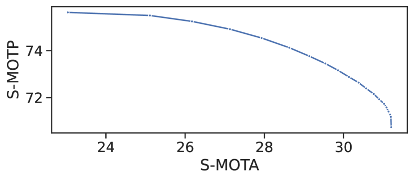
Figure 7: The pareto frontier of optimal S-MOTA vs. S-MOTP optimizing policies. The S-MOTA (x-axis) and S-MOTP (y-axis) of optimal policies with gradually varying weights (blue curve) from S-MOTP to S-MOTA.

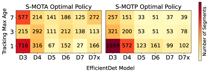
Figure 8: Different policy strategies are needed to optimize S-MOTA and S-MOTP. The configuration choice frequency (color intensity) of S-MOTA-optimal policy (left) and of the S-MOTP-optimal policy (right).

Appendix 0.E Study-case video

A video of the study case presented in Sec. 5.3 is attached with the supplementary material (study-case.mp4). Bounding box and ID annotations are added, matching the color schema of the line-plot that shows the S-MOTA scores of the different policies.

The 10-12 second mark in the video illustrates a large difference between the Octopus policy (green) and the global best policy (black). This difference occurs because the Octopus policy successfully tracks obstacles adjacent to the road on the left and even more on the right that the global best policy does not.

Appendix 0.F t-SNE visualization

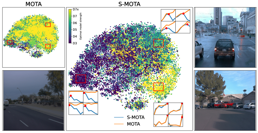
Figure 9: MOTA and S-MOTA responses in different regions of the t-SNE plot, with video-segment visualization. This figure illustrates the following: (i) The t-SNE figures presented in Fig. 5 (ii) Three line-plot quartets, illustrating the MOTA and S-MOTA response (y-axis) of nearby points in the figure to detection model size (x-axis), (iii) A visualization of a representative scenario for each quartet.

We present an expanded analysis of the t-SNE plot in Sec. 5.3. The figure is presented again in Figure 9 with more annotations.

Proximity in score space. Three distinct regions in the t-SNE plot are selected and marked with red rectangles in Figure 9. Four points, representing four 1-second video segments, are selected in each region. The MOTA and S-MOTA scores (y-axis) of increasing detection model size (x-axis) are plotted for these scenarios, following the same methodology as Figure 1(b) and Figure 2 in Sec. 1. The y-axis ticks and scale are omitted to emphasize that nearby video segments have similar, normalized, MOTA and S-MOTA response to the metaparameters. These scenarios, therefore, also tend to be optimized by the same metaparameter values.

Case studies. We perform an in-depth analysis of a video segment selected from each of the three regions indicated in red in Figure 9.

Bottom-left: Turning in difficult conditions. The ego-vehicle turns left into a highway. Larger models cannot detect the parked cars in the background, and therefore do not boost offline MOTA over smaller models. At the same time, vehicle turning induces high obstacle-displacement in the frame, causing accuracy deterioration from higher inference latency. This scene is both very difficult (minimal offline MOTA boost from bigger models) and fast (high accuracy deterioration).

Bottom-right: Slow movement towards partially-occluded vehicles. Stronger models better detect the partially-occluded parked vehicles. The slow ego-vehicle movement towards non-moving obstacles induces minimal obstacle-displacement and therefore negligible accuracy degradation.

Top-right: A mix of still and moving obstacles. The vehicle is standing at an intersection. Still or parked cars on the road are mixed with fast-moving pedestrians. The intermediate-size models, EfficientDet-D5 and D6, detect most of the still obstacles and are able to keep up with the fast-moving pedestrians. Larger models (EfficientDet-D7 and D7x), however, introduce too much inference runtime delay in tracking the moving pedestrians, and sustain more severe accuracy deterioration as a result.

Taken together, these examples illustrate that the environment context can be used to infer MOTA and S-MOTA response to the metaparameters. This then enables test-time S-MOTA optimization by dynamically tuning the metaparameters.

Appendix 0.G Full Centroid Visualization

Full score space clustering analysis. The clustering analysis discussed in Sec. 5.3 (Figure 6) is extended to all eight centroids, shown in Figure 10. Several clusters present similar, though slightly shifted behavior, to the ones presented in the body of the paper. For example, cluster centroids 1, 5, and 8 represent environments with varying S-MOTA response to increasing latency. This demonstrates that the performance penalty (degradation) may occur at different stages as the model size increases. Clusters 3, 4, and 6 show similar improvement in S-MOTA with larger models, though in cluster 6, the performance drops for the two largest models, i.e., EfficientDet-D7 and D7x. These models’ predictions are evaluated 3 frames away from the ground truth, whereas the rest of the models are evaluated up to 2 frames away. This may raise the possibility that the increase in frame gap from the ground truth causes a more significant degradation to S-MOTA in cluster 4 if it contains faster moving scenes than cluster 6.

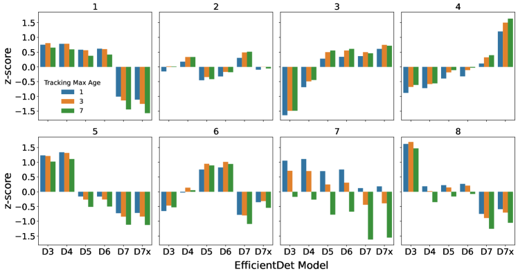
Figure 10: All eight centroids in the clustering analysis performed in Sec. 5.3.

Cluster scenario visualization. Curated videos of several of the clusters’ video segments are attached to the supplementary material (cluster-{4, 7, 8}.mp4) The cluster numbers correspond to the centroid number plotted in Fig. 10.

When comparing clusters 4 and 8, we observe a clear trend: (i) video segments with a preference for larger models (cluster 4) show more subdued obstacle displacement from the ego vehicle camera’s perspective and (ii) the opposite in video segments with preference for smaller models (cluster 8).

In cluster 7, a lower tracking maximum age has better performance. Here, we observe video segments with two primary modes of obstacle behavior: (i) occlusions or obstacles leaving the scene, and (ii) very fast obstacle movement, where the IoU of the obstacle to its previous location is small, causing SORT [2] to do an ID switch. In both cases, maintaining the old tracklets for a shorter amount of time reduces false positives and improves performance.

These observations illustrate the idea that visible properties of the environment context may be leveraged to discern the mode of metaparameter score behavior. These properties are used as features in Octopus to optimize S-MOTA at test time.

Appendix 0.H Ranking Implementation Ablations

We conduct an ablation study of the experimental setup and the design choices.

Baseline subtraction. As a variance reduction technique, we consider regressing over the relative score improvement from $h^{global}$ instead of absolute scores as described in 4.1. Thus, we avoid dedicating model capacity to learn environment “difficulty” properties, which apply to all configurations in a manner that does not change their score order. As this distinction is not relevant for predicting configuration order, it only introduces noise to the downstream ranking task [35]. Accordingly, in Table 8, we observe a $0.3$ point decrease in S-MOTA score on the Waymo dataset when baseline subtraction is ablated.

Classification vs. regression. We compare the regress-then-rank approach described in Sec. 4.1 against the classification formulation (using Random Forests). This approach directly predicts the metaparameter values of the best configuration from the environment features using $m$ classifiers for each of the $m$ metaparameters. In Table 8 we show the resulting score in "classification (joint)", indicating a reduced score compared to regression with baseline subtraction.

Independent vs. joint metaparameter optimization. We examine the degree of independence between metaparameter choices in the optimization process. To this end, we consider a new setting "classification (independent)" in Table 8. This is done by separately learning to predict the value of each metaparameter, while holding the other metaparameter values constant (in essence assuming convexity). We show that joint classification performs $0.4$ S-MOTA points better than independent.

Table 8: Comparing configuration ranking approaches

Method	S-MOTA$\uparrow{}$	S-MOTP$\uparrow{}$	S-FN$\downarrow{}$	S-FP$\downarrow{}$	S-IDsw$\downarrow{}$
Regression w/ baseline subtraction	27.9	72.3	31489	608870	8966
Regression w/o baseline subtraction	27.6	72.5	31405	610617	8982
Classification (independent)	27.2	72.9	32725	615537	9326
Classification (joint)	27.6	72.7	35107	611196	8829

Appendix 0.I Policy Design Using Neural Networks

The key idea in this study is that the environment context can be leveraged to optimize streaming tracking accuracy at test time. The Octopus policy model presented is implemented using engineered features and random forest regression. A natural question is whether the policy performance can be improved using deep neural networks. To this end, we evaluated policy design that incorporates a conventional, convolutional neural network (CNN) [10] as well. We found that performance is on par with the global best policy, much worse than the solution using engineered features (see Table 9). In order to get good performance, we believe that the model needs to predict features at the granularity of instance-level motion (e.g. instance-flow [38]) because the tracking score that is being predicted is defined at this granularity. We believe that the model does not get good score because it does not capture these features well. Further investigation is needed.

0.I.1 Methodology

We use a ResNet50 backbone [10] that takes as input the middle frame of each 1-second video segment and classifies the best configuration using a new MLP. The backbone is pretrained using QDTrack [27] on the BDD100k dataset [36] (QDTrack’s zero-shot accuracy on Waymo is 40.3, on par with the optimal policy score in offline settings). The backbone output is average-pooled and fed to an MLP of width of 256 with one hidden layer. The MLP output is fed into separate linear layers that generate the logits for each metaparameter in order to separately classify the values of the optimal configuration. This follows the methodology described in Appendix 0.H. The model is trained using the cross-entropy loss on the Waymo dataset, using the methodology described in Sec. 5.1. The logits are initialized with a small bias so that the model behaves like the global best policy at the start of training. The model is trained using AdamW [19] with a learning rate of 1e-4 and weight decay of 0.01 for 10 epochs.

0.I.2 Results

The results are shown in Table 9. The CNN achieves negligible performance improvement over the global best policy.

Table 9: Neural-network based policy performance

Method	S-MOTA$\uparrow{}$	S-MOTP$\uparrow{}$	S-FP$\downarrow{}$	S-FN$\downarrow{}$	S-IDsw$\downarrow{}$
Global best	25.1	72.2	33616	633159	11212
Neural network based policy	25.2	72.3	45658	611827	8056

Appendix 0.J Faster hardware simulation

Hardware performance is expected to improve over time. We therefore evaluate Octopus on faster hardware execution by simulating 50% faster inference of the detection model measured on the V100 GPU. We repeat the evaluation on the Argoverse dataset described in Sec. 5.2, showing the results in Table 10. The results show that the Octopus policy with closed-loop prediction outperforms the global best static policy by 2.8 S-MOTA, up from the 1.7 S-MOTA result using the V100 GPU latency readings.

Table 10: Performance on Argoverse with 50% faster GPU inference

Method	S-MOTA$\uparrow{}$	S-MOTP$\uparrow{}$	S-FP$\downarrow{}$	S-FN$\downarrow{}$	S-IDsw$\downarrow{}$
Global best	54.5	77.3	8508	44965	1173
Optimal	63.7	75.5	6897	36634	649
Optimal from the prev. segment	57.6	75.5	9655	40800	776
Octopus with:
Ground truth from current segment	59.3	75.9	7951	40405	815
Ground truth from prev. segment	57.9	76.3	7988	41553	958
Prediction from prev. segment	57.3	76.4	7911	42489	958

References

- [1] Baldock, R., Maennel, H., Neyshabur, B.: Deep learning through the lens of example difficulty. Advances in Neural Information Processing Systems 34, 10876–10889 (2021)
- [2] Bewley, A., Ge, Z., Ott, L., Ramos, F., Upcroft, B.: Simple Online and Realtime Tracking. In: Proceedings of the 23th IEEE International Conference on Image Processing (ICIP). pp. 3464–3468 (2016)
- [3] Bochkovskiy, A., Wang, C.Y., Liao, H.Y.M.: YOLOv4: Optimal Speed and Accuracy of Object Detection. arXiv preprint arXiv:2004.10934 (2020)
- [4] Breiman, L.: Random forests. Machine learning 45(1), 5–32 (2001)
- [5] Chang, M.F., Lambert, J., Sangkloy, P., Singh, J., Bak, S., Hartnett, A., Wang, D., Carr, P., Lucey, S., Ramanan, D., et al.: Argoverse: 3D Tracking and Forecasting with Rich Maps (2019)
- [6] Courdier, E., Fleuret, F.: Real-time segmentation networks should be latency aware. In: Proceedings of the Asian Conference on Computer Vision (2020)
- [7] Dendorfer, P., Rezatofighi, H., Milan, A., Shi, J., Cremers, D., Reid, I., Roth, S., Schindler, K., Leal-Taixé, L.: Mot20: A benchmark for multi object tracking in crowded scenes. arXiv preprint arXiv:2003.09003 (2020)
- [8] Gog, I., Kalra, S., Schafhalter, P., Wright, M.A., Gonzalez, J.E., Stoica, I.: Pylot: A Modular Platform for Exploring Latency-Accuracy Tradeoffs in Autonomous Vehicles. In: Proceedings of IEEE International Conference on Robotics and Automation (ICRA) (2021)
- [9] Han, S., Pool, J., Tran, J., Dally, W.J.: Learning both Weights and Connections for Efficient Neural Networks. In: Proceedings of the 28th International Conference on Neural Information Processing (NeurIPS). pp. 1135–1143 (2015)
- [10] He, K., Zhang, X., Ren, S., Sun, J.: Deep residual learning for image recognition. In: Proceedings of the IEEE conference on computer vision and pattern recognition. pp. 770–778 (2016)
- [11] Huang, J., Rathod, V., Sun, C., Zhu, M., Korattikara, A., Fathi, A., Fischer, I., Wojna, Z., Song, Y., Guadarrama, S., Murphy, K.: Speed/Accuracy Trade-Offs for Modern Convolutional Object Detectors. In: Proceedings of the IEEE Conference on Computer Vision and Pattern Recognition (CVPR) (2017)
- [12] Jiang, J., Ananthanarayanan, G., Bodik, P., Sen, S., Stoica, I.: Chameleon: Scalable Adaptation of Video Analytics. In: Proceedings of the 2018 Conference of the ACM Special Interest Group on Data Communication (SIGCOMM). pp. 253–266 (2018)
- [13] Leal-Taixé, L., Milan, A., Schindler, K., Cremers, D., Reid, I., Roth, S.: Tracking the trackers: an analysis of the state of the art in multiple object tracking. arXiv preprint arXiv:1704.02781 (2017)
- [14] Li, M., Wang, Y., Ramanan, D.: Towards Streaming Perception. In: Proceedings of the European Conference on Computer Vision (ECCV) (2020)
- [15] Lin, J., Rao, Y., Lu, J., Zhou, J.: Runtime Neural Pruning. In: Proceedings of the 31st International Conference on Neural Information Processing Systems (NeurIPS). pp. 2178–2188 (2017)
- [16] Lin, S.C., Zhang, Y., Hsu, C.H., Skach, M., Haque, M.E., Tang, L., Mars, J.: The Architectural Implications of Autonomous Driving: Constraints and Acceleration. In: Proceedings of the 23rd International Conference on Architectural Support for Programming Languages and Operating Systems (ASPLOS). pp. 751–766 (2018)
- [17] Liu, T.Y., et al.: Learning to rank for information retrieval. Foundations and Trends® in Information Retrieval 3(3), 225–331 (2009)
- [18] Liu, W., Anguelov, D., Erhan, D., Szegedy, C., Reed, S., Fu, C.Y., Berg, A.C.: SSD: Single shot multibox detector. In: Proceedings of the European Conference on Computer Vision (ECCV). pp. 21–37. Springer (2016)
- [19] Loshchilov, I., Hutter, F.: Decoupled weight decay regularization. arXiv preprint arXiv:1711.05101 (2017)
- [20] Luiten, J., Osep, A., Dendorfer, P., Torr, P., Geiger, A., Leal-Taixé, L., Leibe, B.: Hota: A higher order metric for evaluating multi-object tracking. International journal of computer vision 129(2), 548–578 (2021)
- [21] Luo, J.H., Wu, J., Lin, W.: Thinet: A Filter Level Pruning Method for Deep Neural Network Compression. In: Proceedings of the IEEE/CVF Conference on Computer Vision and Pattern Recognition (CVPR). pp. 5058–5066 (2017)
- [22] Milan, A., Leal-Taixé, L., Reid, I., Roth, S., Schindler, K.: Mot16: A benchmark for multi-object tracking. arXiv preprint arXiv:1603.00831 (2016)
- [23] Mittal, G., Liu, C., Karianakis, N., Fragoso, V., Chen, M., Fu, Y.: HyperSTAR: Task-Aware Hyperparameters for Deep Networks. In: Proceedings of the IEEE/CVF Conference on Computer Vision and Pattern Recognition (CVPR). pp. 8736–8745 (2020)
- [24] Nishi, K., Shimosaka, M.: Fine-Grained Driving Behavior Prediction via Context-Aware Multi-Task Inverse Reinforcement Learning. In: 2020 IEEE International Conference on Robotics and Automation (ICRA). pp. 2281–2287. IEEE (2020)
- [25] NVIDIA: Tensor RT. https://developer.nvidia.com/tensorrt
- [26] Padilla, R., Passos, W.L., Dias, T.L., Netto, S.L., da Silva, E.A.: A comparative analysis of object detection metrics with a companion open-source toolkit. Electronics 10(3), 279 (2021)
- [27] Pang, J., Qiu, L., Li, X., Chen, H., Li, Q., Darrell, T., Yu, F.: Quasi-dense similarity learning for multiple object tracking. In: Proceedings of the IEEE/CVF Conference on Computer Vision and Pattern Recognition. pp. 164–173 (2021)
- [28] Park, E., Ahn, J., Yoo, S.: Weighted-entropy-based Quantization for Deep Neural Networks. In: Proceedings of the IEEE/CVF Conference on Computer Vision and Pattern Recognition (CVPR). pp. 5456–5464 (2017)
- [29] Pleskac, T.J., Busemeyer, J.R.: Two-stage dynamic signal detection: a theory of choice, decision time, and confidence. Psychological review 117(3), 864 (2010)
- [30] Shen, H., Han, S., Philipose, M., Krishnamurthy, A.: Fast Video Classification via Adaptive Cascading of Deep Models. In: Proceedings of the IEEE Conference on Computer Vision and Pattern Recognition (CVPR). pp. 3646–3654 (2017)
- [31] Tan, M., Pang, R., Le, Q.V.: EfficientDet: Scalable and Efficient Object Detection. In: Proceedings of the IEEE Conference on Computer Vision and Pattern Recognition (CVPR) (2020)
- [32] Wang, X., Yu, F., Dou, Z.Y., Darrell, T., Gonzalez, J.E.: Skipnet: Learning Dynamic Routing in Convolutional Networks. In: Proceedings of the European Conference on Computer Vision (ECCV). pp. 409–424 (2018)
- [33] Waymo Inc.: Waymo Open Dataset. https://waymo.com/open/
- [34] Xu, Y., Wang, Y., Zhou, A., Lin, W., Xiong, H.: Deep Neural Network Compression with Single and Multiple Level Quantization. In: Proceedings of the AAAI Conference on Artificial Intelligence. vol. 32 (2018)
- [35] Yogatama, D., Mann, G.: Efficient transfer learning method for automatic hyperparameter tuning. In: Artificial intelligence and statistics. pp. 1077–1085. PMLR (2014)
- [36] Yu, F., Xian, W., Chen, Y., Liu, F., Liao, M., Madhavan, V., Darrell, T.: Bdd100k: A diverse driving video database with scalable annotation tooling. arXiv preprint arXiv:1805.04687 2(5), 6 (2018)
- [37] Zhao, R., Hu, Y., Dotzel, J., De Sa, C., Zhang, Z.: Improving Neural Network Quantization without Retraining using Outlier Channel Splitting. In: International Conference on Machine Learning (ICML). pp. 7543–7552 (2019)
- [38] Zhou, X., Koltun, V., Krähenbühl, P.: Tracking objects as points. In: Proceedings of the European Conference on Computer Vision (ECCV). pp. 474–490. Springer (2020)