Periodic Coupled-Cluster Green’s Function for Photoemission Spectra of Realistic Solids
Abstract
We present an efficient implementation of coupled-cluster Green’s function (CCGF) method for simulating photoemission spectra of periodic systems. We formulate the periodic CCGF approach with Brillouin zone sampling in Gaussian basis at the coupled-cluster singles and doubles (CCSD) level. To enable CCGF calculations of realistic solids, we propose an active-space self-energy correction scheme by combining CCGF with cheaper many-body perturbation theory (GW) and implement the model order reduction (MOR) frequency interpolation technique. We find that the active-space self-energy correction and MOR techniques significantly reduce the computational cost of CCGF while maintaining the high accuracy. We apply the developed CCGF approaches to compute spectral properties and band structure of silicon (Si) and zinc oxide (ZnO) crystals using triple- Gaussian basis and medium-size -point sampling, and find good agreement with experimental measurements.
Accurate first-principles simulation of spectral properties is key to understanding and designing solid-state materials for energy, catalysis, and quantum technologies. Density functional theory (DFT) [1] has been the workhorse for calculating band structure of solids due to its low cost, although it suffers from systematic errors and Kohn-Sham orbital energies do not formally describe the quasiparticle energies [2, 3, 4]. Correlated Green’s function methods provide a formal route to computing photoemission spectra beyond DFT [5, 6, 7, 8, 9, 10, 11, 12]. One of the most successful Green’s function approaches for this task is the many-body perturbation theory, or GW [13, 14, 15, 16, 17, 18]. Owing to proper treatment of dielectric screening, the GW theory in its one-shot formulation predicts accurate band gaps of weakly-correlated semiconductors and insulators. On the other hand, no GW formulation (e.g., self-consistency, DFT starting point, vertex correction) is known to be consistently reliable across weakly and strongly correlated materials. To achieve quantitative description of charged excitations beyond GW, one promising framework is the Green’s function embedding such as dynamical mean-field theory (DMFT) [19, 20, 21, 22] and self-energy embedding theory (SEET) [23, 24], but other approximations must be invoked, which require careful treatment.
Hence, it is necessary to develop higher-order ab initio Green’s function methods for periodic systems. Recently, the coupled-cluster (CC) theory has been extended to compute ground-state and excited-state properties of realistic solids and shows great promise in simulating both weakly (e.g., silicon) and strongly (e.g., nickel oxide) correlated materials [25, 26, 27, 28, 29]. Meanwhile, molecular coupled-cluster Green’s function (CCGF) implementations have been developed for studying photoelectron spectra of molecules and models [30, 31, 32, 33, 34, 35] and solving impurity problems in ab initio DMFT calculations [36, 21, 22, 37, 38]. However, efficient periodic CCGF implementation capable of simulating photoemission spectra and band structure of realistic materials is not yet available due to high computational cost [39]. In this work, we fill this gap by developing accelerated periodic CCGF approach in Gaussian basis with Brillouin zone sampling.
We start with a description of molecular CCGF theory [32, 33, 36]. The one-particle Green’s function of a given system in frequency (energy) domain is defined as:
| (1a) | ||||
| (1b) | ||||
where and are addition (EA) and removal (IP) parts of Green’s function, is the ground-state wave function, is the Hamiltonian, is the ground-state energy, and is a small broadening factor. and are annihilation and creation operators on orbitals and . In coupled-cluster theory, the CC ground-state wave function is parameterized as
| (2) |
with as the cluster excitation operator and as the Hartree-Fock determinant. In this work, we truncate the operator at the singles and doubles level (i.e., CCSD). The CC bra state is parameterized differently as:
| (3) |
where is the de-excitation operator. Inserting Eq. 2 and Eq. 3 into Eq. 1, one arrives at the CCGF equations:
| (4a) | ||||
| (4b) | ||||
where similarity transformed operators are defined as:
| (5) |
To efficiently solve Eq. 4, we define vectors and :
| (6a) | ||||
| (6b) | ||||
so that Eq. 4 becomes
| (7a) | ||||
| (7b) | ||||
To solve the set of linear equations in Eq. 6, and are parameterized in the EOM-CCSD (equation-of-motion CCSD) approximation [40, 41]:
| (8a) | ||||
| (8b) | ||||
where contains one-particle () and two-particle one-hole () terms and contains and terms. We use the sparse linear equation solver GCROT(m,k) [42] as implemented in SciPy [43] to solve Eqs. 6 and 8.
For periodic systems, we work explicitly with -point (Brillouin zone) sampling in the reciprocal space. The -point CCGF equation is
| (9a) | ||||
| (9b) | ||||
From the Green’s function, one obtains momentum-dependent spectral function
| (10) |
whose trace defines density of states (DOS).
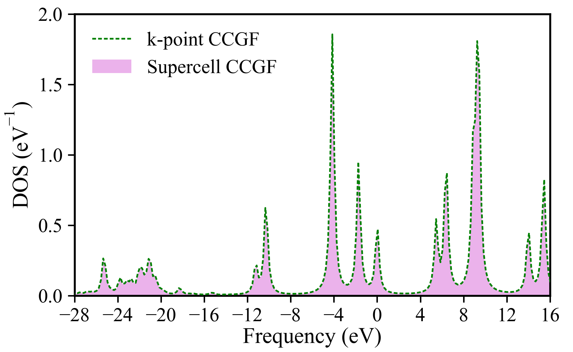
We implemented -point CCGF approach in PySCF quantum chemistry software package [44] using a hybrid MPI+OpenMP parallelization scheme. To avoid solving -point equations, we approximate the amplitudes as the complex conjugate of amplitudes. We evaluated the accuracy of this approximation against an exact supercell (molecular) CCGF calculation on the diamond crystal and found excellent agreement (Fig. S1).
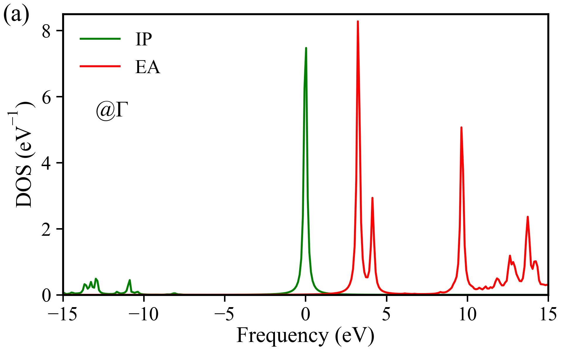
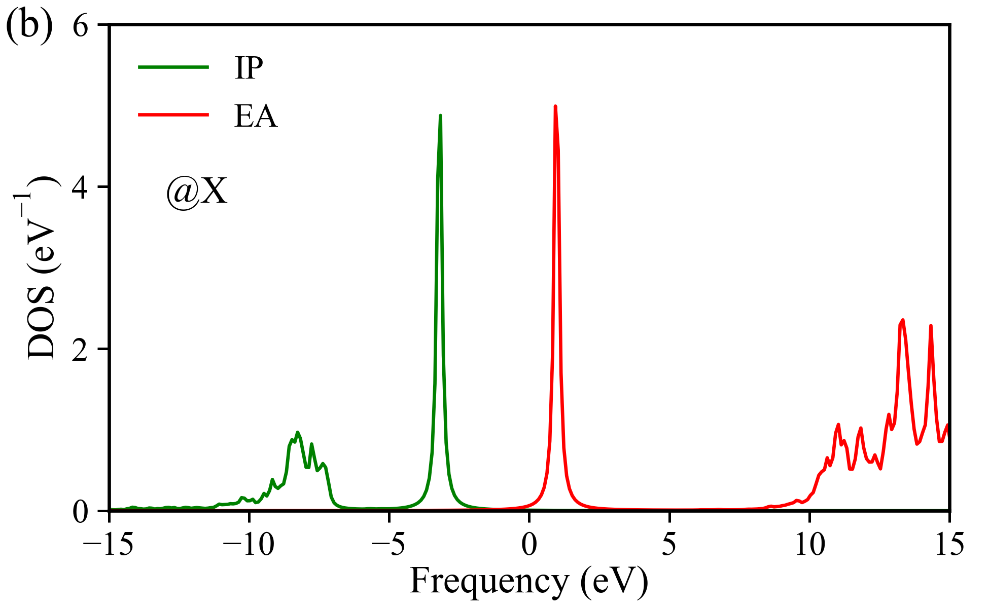
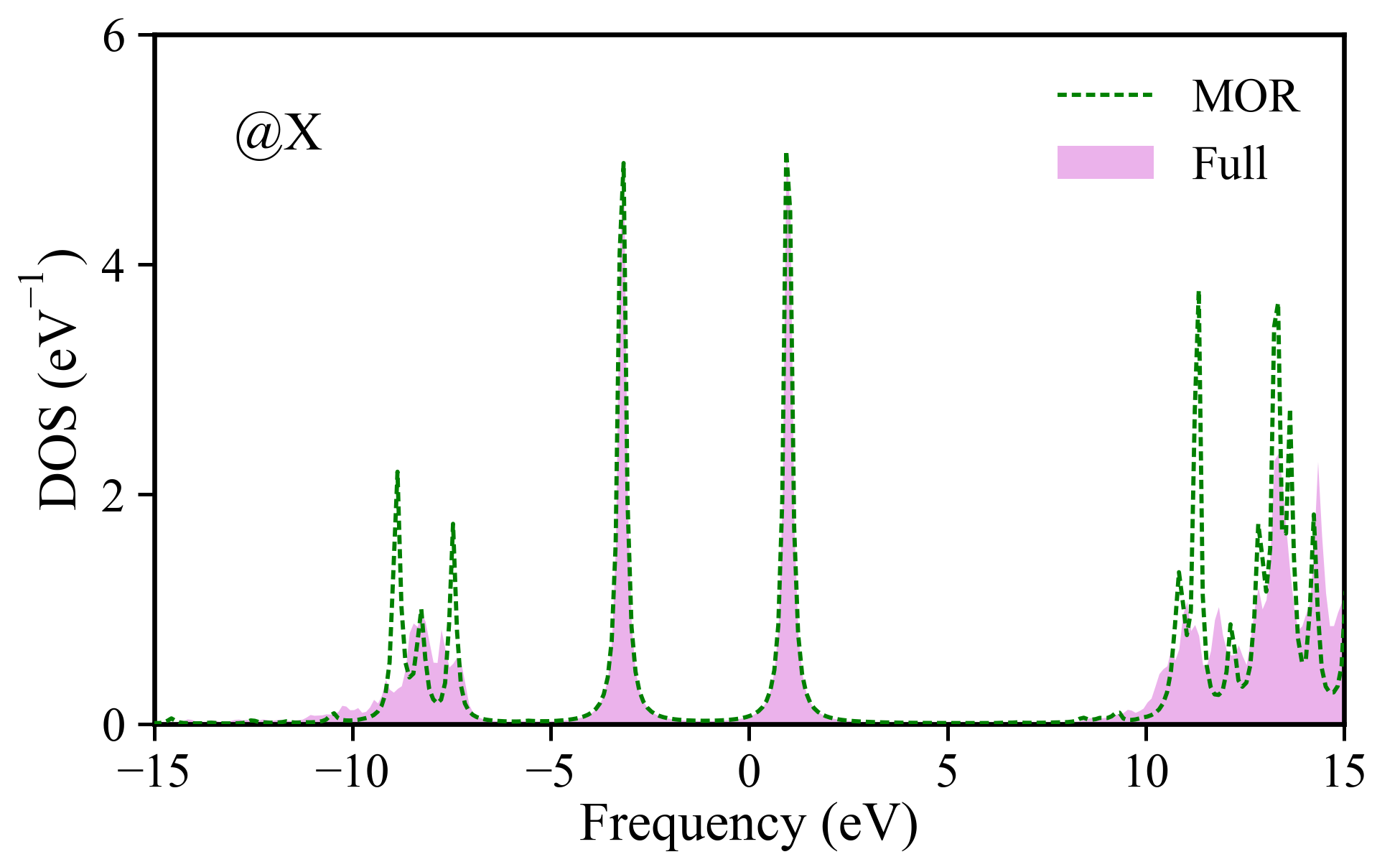
In Fig. 1(a) and 1(b), we show momentum-dependent density of states (DOS) of Si computed by -point CCGF method with GTH-HF pseudopotential and GTH-DZVP basis set [45, 46] as well as -point sampling. Because our periodic CCGF approach is formulated on real-frequency axis, it is capable of computing photoemission spectra of valence, core, and high-virtual bands, which involve quasiparticle and satellite (e.g., [-15, -10] eV and [10, 15] eV in Fig. 1(a)) peaks.
Although it is now possible to perform small -point CCGF calculations, the high computational scaling of periodic CCGF prohibits its application to more complex materials. At each -point, frequency , and Green’s function column/row (for EA/IP), the scaling of the EA part is and the scaling of the IP part is . are the number of sampled -points, occupied orbitals, and virtual orbitals (per unit cell, respectively). The overall cost for computing and matrices for all -points are thus and , with and as the sampled frequency points. In the rest of this Letter, we describe acceleration techniques to reduce and .
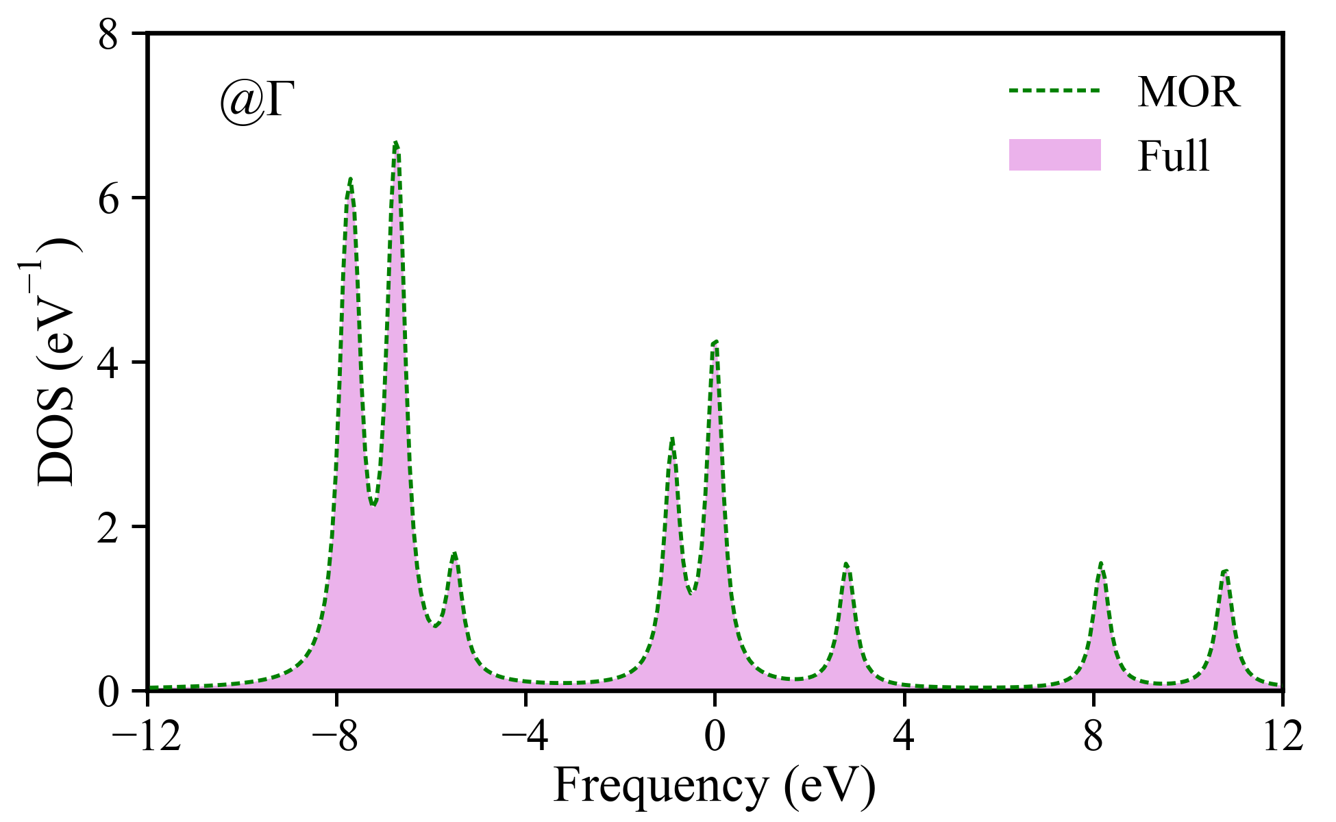
Model order reduction. To obtain high resolution in photoemission spectra, one usually needs to perform CCGF calculations on hundreds of frequency points. This large prefactor can be significantly lowered by the model order reduction (MOR) method, which is a technique for reducing computational complexity of mathematical models and has been successfully applied to compute X-ray absorption spectra and CCGF for molecules [47, 34]. We refer the readers to Ref. [34] for details of the MOR-CCGF implementation. Briefly speaking, in MOR-CCGF, one computes the full CCGF (Eq. 6) on a small set of selected frequency points (e.g., ), then uses solved or to construct a subspace. The original effective Hamiltonian () is then projected onto the subspace to form a much smaller model with dimension of . One finally solves CCGF equations on all frequency points () using this reduced model, which has negligible cost. Thus, MOR is a frequency interpolation (sometimes extrapolation) technique that decreases the prefactor from to .
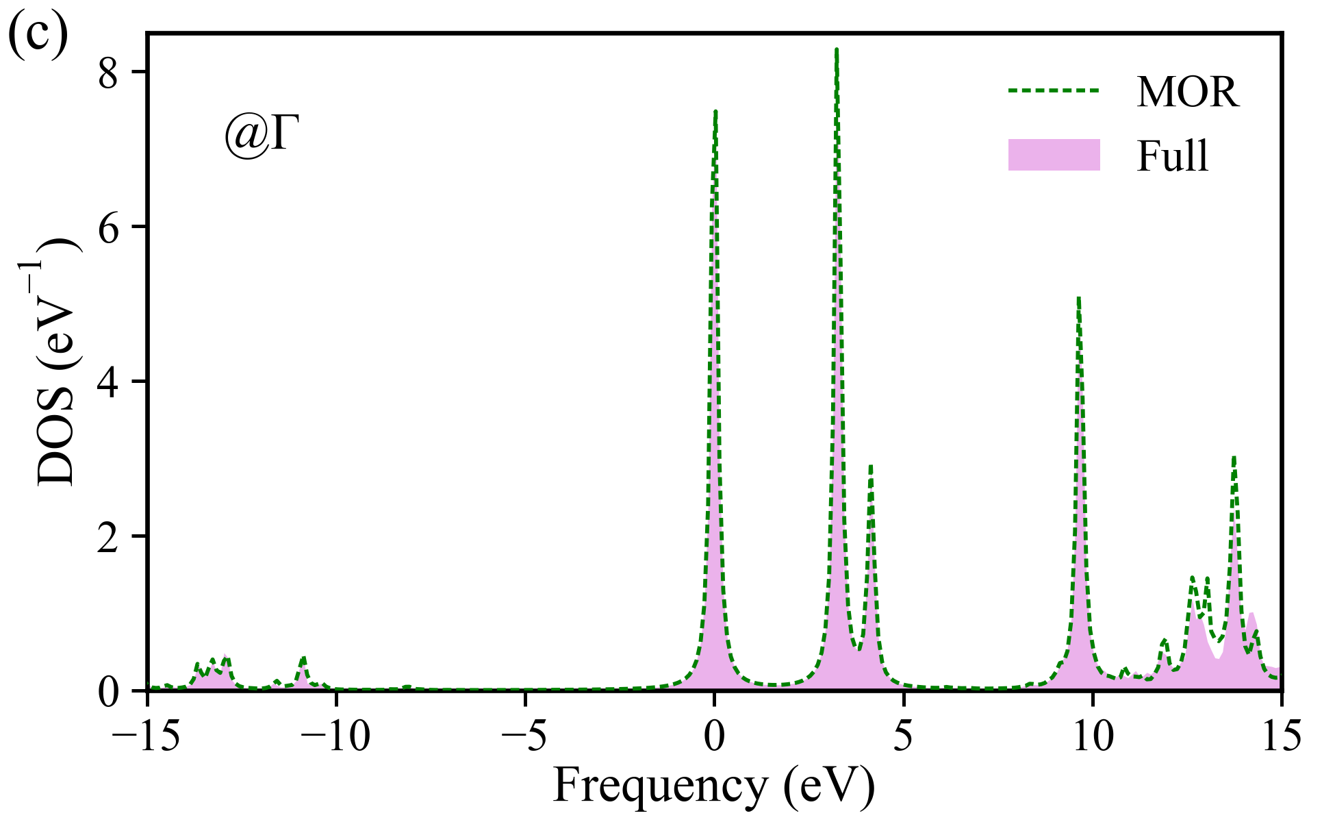
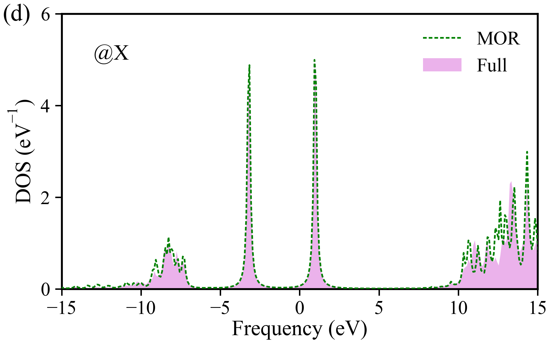
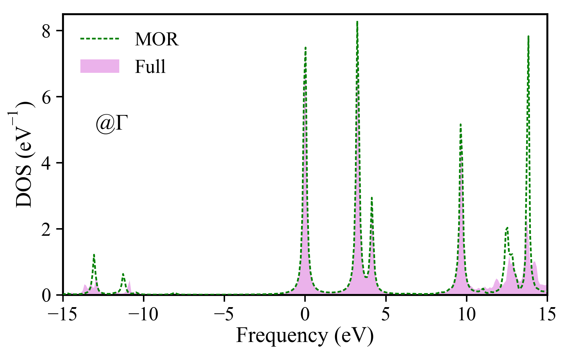
We implemented the MOR technique within our periodic CCGF code and tested the accuracy of MOR-CCGF on Si. In Fig. 1(c) and 1(d), we chose (equally distributed on [-15,0] eV for IP and [0,15] eV for EA) and respectively (meaning the cost of MOR-CCGF is of full CCGF). MOR-CCGF reproduces the main quasiparticle peaks around Fermi level perfectly compared to full CCGF calculations. Even the satellite peaks at [-15, -5] eV and [10, 15] eV are captured accurately. If one focuses only on the valence peaks, we found that is enough to yield highly accurate CCGF DOS (see Fig. S2).
Active-space self-energy correction. Following the idea of frozen natural orbital coupled-cluster theory [48, 49, 50], we develop an active-space approach to reduce the number of orbitals in periodic CCGF calculations. Specifically, we show an efficient combination of CCGF and GW methods through a self-energy correction scheme.
We first perform a GW calculation on the system using Gaussian-based G0W0 method developed by one of the authors (T.Z.) [17]. Throughout this Letter, we employ the one-shot G0W0@HF method that scales as . From the G0W0@HF calculation, we obtain the GW density matrix using a linearized GW density matrix formalism [51] which guarantees conserving particle number. The GW density matrix is then diagonalized to derive a set of natural orbitals:
| (11) |
where is the natural orbital (NO) coefficient and is the occupation number of NOs. We then select most partially occupied orbitals to form an active space and perform periodic CCGF calculation. Because , the computational cost of CCGF is approximately decreased from to . We note that we keep active space the same size for all -points to simplify the implementation.
However, this frozen natural orbital scheme does not work well for excited states and truncating the NO basis from to results in a loss of accuracy. To remedy the error, we define a self-energy correction term within the complete active space (CAS):
| (12) |
and transform it back to the full molecular orbital (MO) space
| (13) |
Then the CC+GW Green’s function is computed through Dyson’s equation:
| (14) |
where the GW Green’s function () for the full system is computed when deriving the natural orbital basis. We note that this scheme can also be applied using other low-level theories, such as MP2 or self-consistent GW [52, 53].
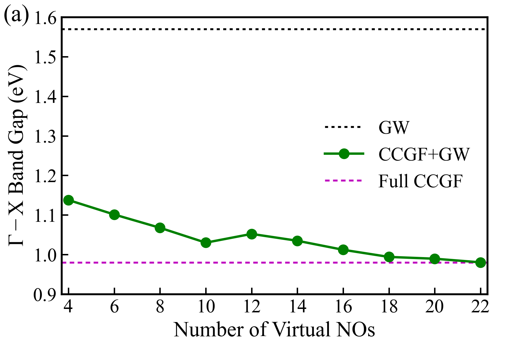
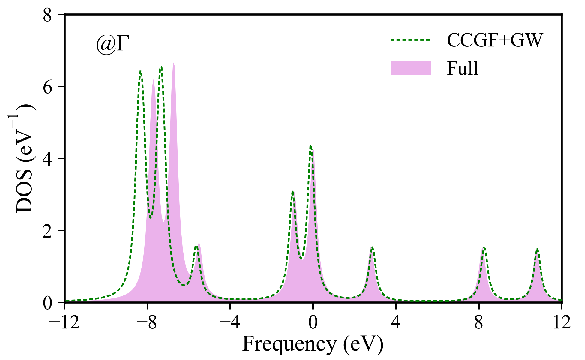
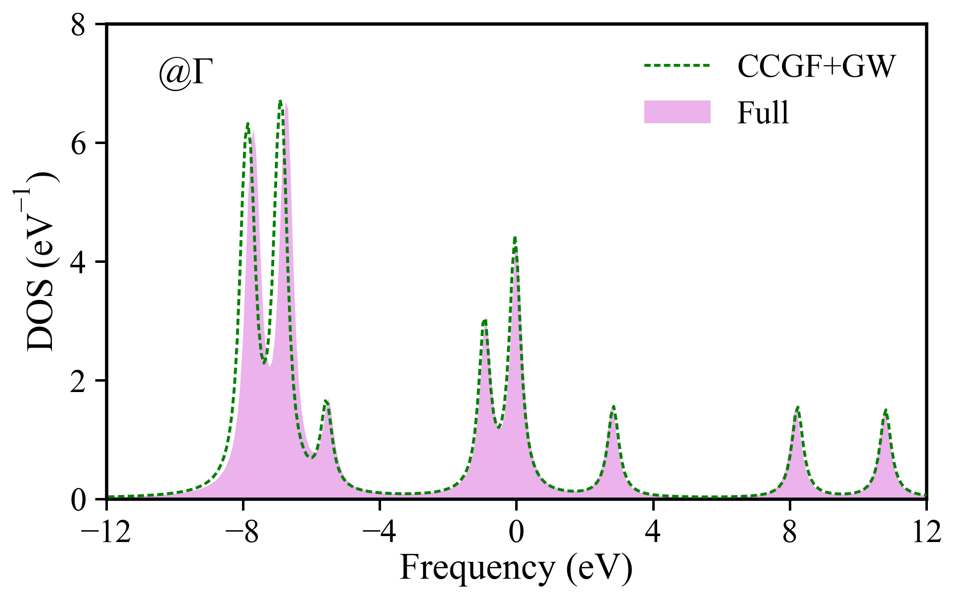
We benchmarked the accuracy of CCGF+GW on Si and wurtzite zinc oxide (ZnO). We used GTH-DZVP basis set and -point sampling for Si and def2-SV(P) basis set [54] and -point sampling for ZnO. In Fig. 2(a), we tested the X band gap of Si using different number of virtual NOs in the active space, while all (4) occupied orbitals are included. As a comparison, the full CCGF and G0W0@HF band gaps are 0.98 eV and 1.57 eV, which correspond to 22 virtual orbitals per unit cell. As the number of active virtual NOs increases, the CCGF+GW band gap quickly converges to the full CCGF result. We find that using only 4 virtual NOs per unit cell, the CCGF+GW band gap is 1.14 eV, only 0.16 eV larger than full CCGF gap. At 10 virtual NOs, the CCGF+GW band gap error is only 0.05 eV (or 5%). We note that for DOS at point, the CCGF+GW calculation with 10 virtual NOs takes 2 hours on 112 CPU cores, while the full CCGF calculation costs 19 hours using same resources.
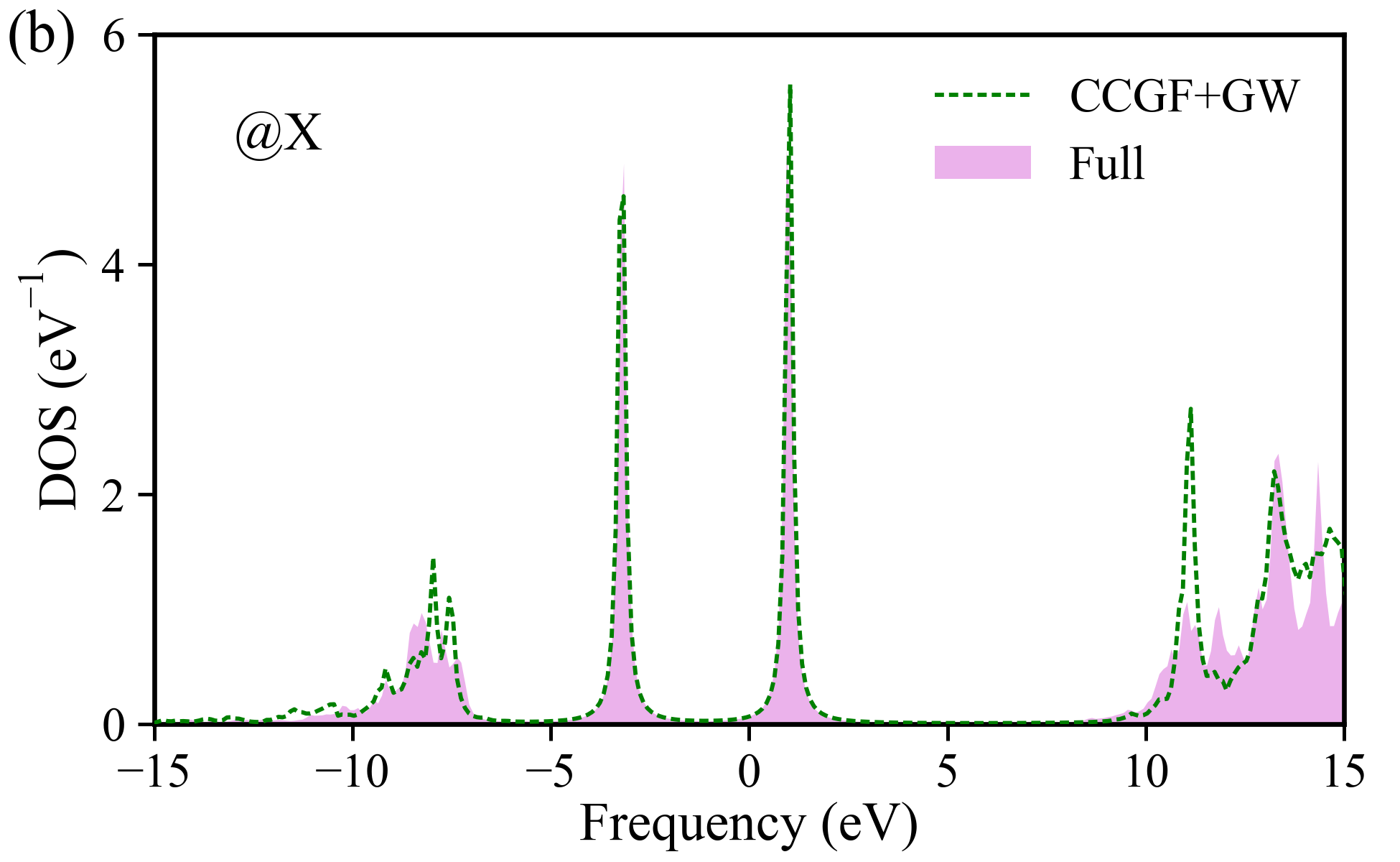
The DOS for Si at X point is presented in Fig. 2(b) using an active space of (8e, 14o) (i.e., 8 electrons and 14 orbitals per unit cell). It is shown that not only the low-energy quasiparticle peaks are accurately described by CCGF+GW, but also the deeper valence and higher virtual spectra are well captured.
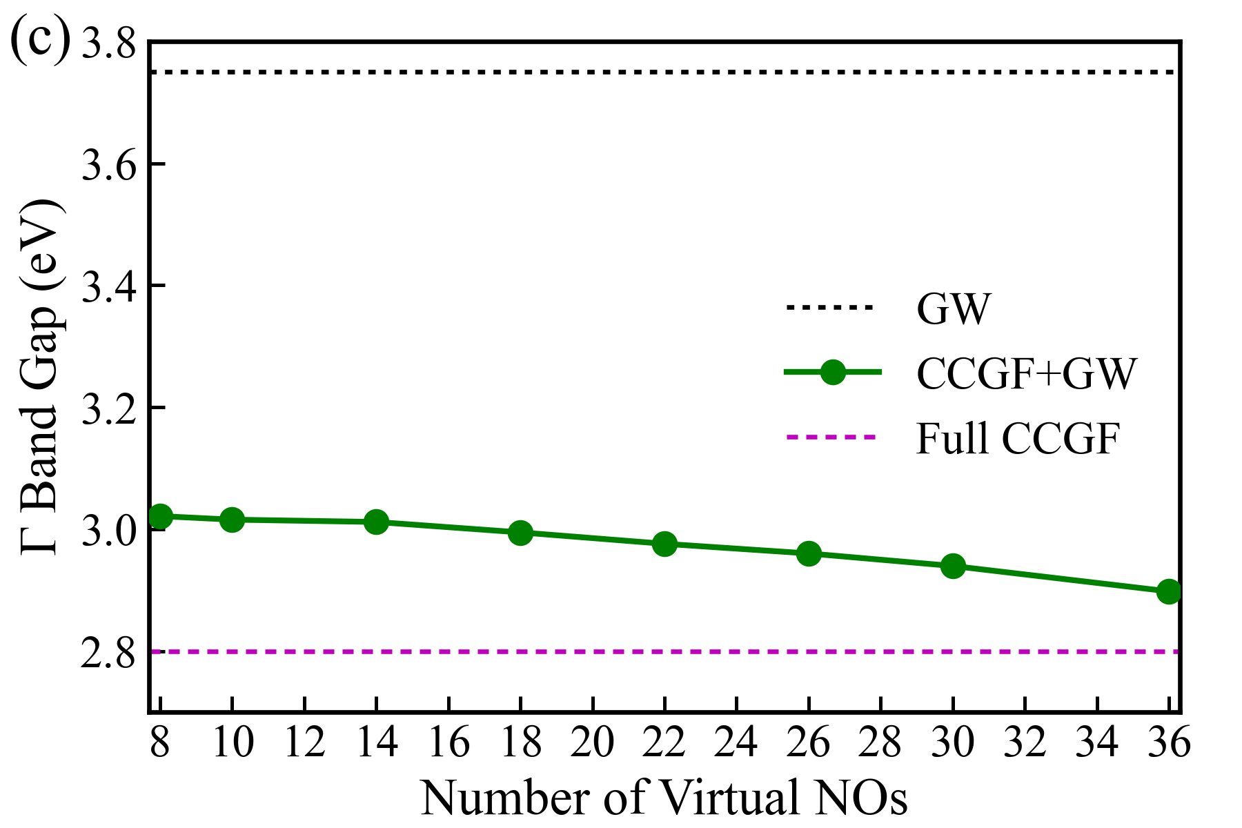
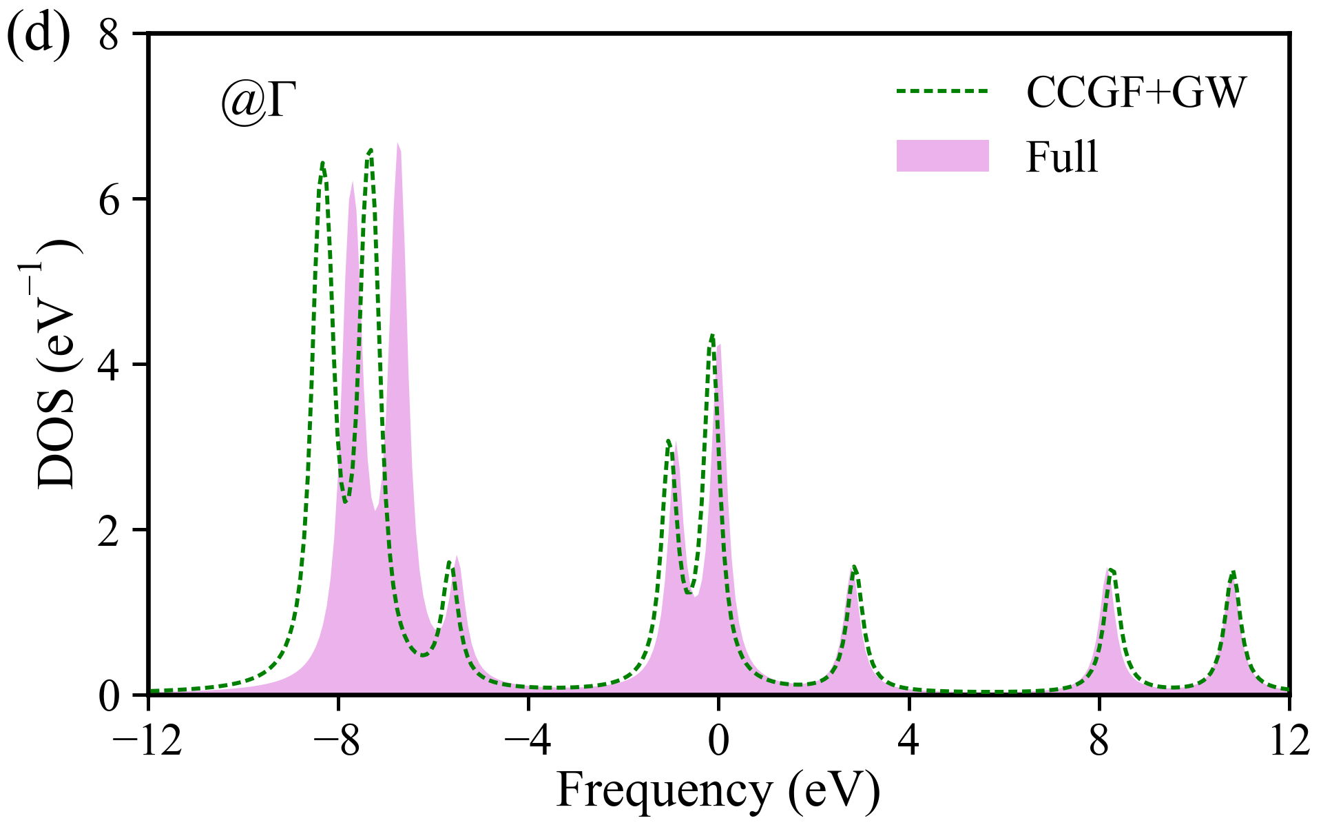
In Fig. 2(c) and 2(d), we present similar tests for ZnO. The full CCGF and G0W0@HF band gap for ZnO are 2.80 eV and 3.75 eV, which correspond to 38 occupied and 38 virtual orbitals per unit cell. Fixing the number of active occupied orbitals to 8 in Fig. 2(c), reasonably accurate band gaps are produced by CCGF+GW. For example, at 10 virtual NOs, the CCGF+GW band gap is 3.02 eV and has 8% relative error compared to full CCGF. More test results on ZnO are available in the SI. The photoemission spectrum computed by (16e, 18o) CCGF+GW also shows good agreement with full CCGF in Fig. 2(d). The discrepancy in the [-10, -6] eV region is likely due to the small number of active occupied orbitals used in CCGF+GW.
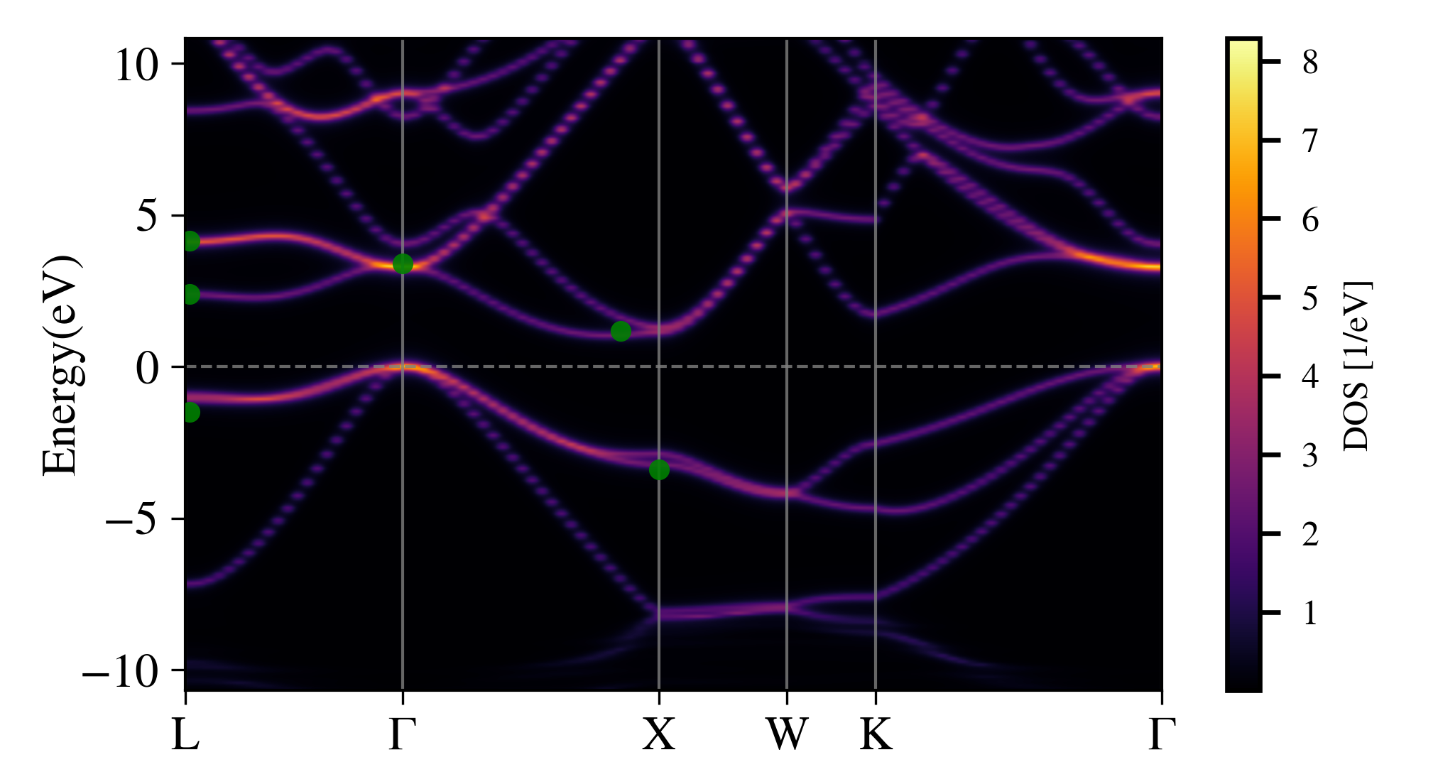
Combining both active-space self-energy correction and MOR techniques, we study Si and ZnO using higher-quality basis set and larger Brillouin zone sampling. For Si, we used the correlation-consistent GTH-cc-pVTZ basis set recently developed by Ye and Berkelbach [55] as well as GTH-HF pseudopotential. We applied MOR-CCGF+GW approach with an active space of (8e, 14o) per unit cell and . Using band interpolation technique based on intrinsic atomic orbital and projected atomic orbital (IAO+PAO) [56, 57, 39], we obtain band structure of Si from MOR-CCGF+GW calculation at -mesh in Fig. 3. We find that the CCGF band structure is in excellent agreement with experimental photoemission data [58].
To obtain Si band gap in the thermodynamic limit (TDL), we performed MOR-CCGF+GW calculations at , , and -meshes, and conducted a finite size extrapolation of band gap with respect to . The results are summarized in Table 1. Furthermore, we applied a correction term at -mesh that accounts for the error introduced by using small active space:
| (15) |
where corresponds to a (8e, 28o) MOR-CCGF+GW calculation and refers to the (8e, 14o) calculation. The final estimated Si band gap is thus
| (16) |
We find that eV and eV, leading to estimated CCGF band gap at 0.98 eV, which is 0.25 eV underestimated compared to the experimental band gap of 1.23 eV (taking zero-point renormalization effect into account). We note that our CCGF band gap is 0.21 eV smaller than EOM-CCSD result (1.19 eV) in Ref. [25], which is mainly caused by the use of different basis sets (GTH-cc-pVTZ vs. GTH-TZVP).
| TDL+ | Expt. | ||||
| Si | 0.78 | 0.85 | 0.89 | 0.98 | 1.23 |
| TDL+ | Expt. | ||||
| ZnO | 2.39 | 3.47 | 3.97 | 4.94 | 3.60 |
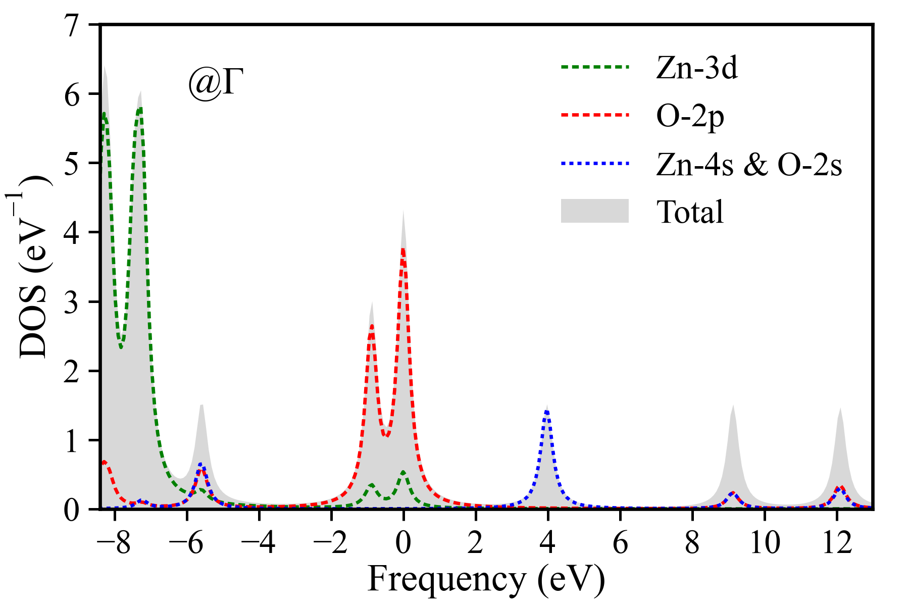
We then report MOR-CCGF+GW results on wurtzite ZnO, using an active space of (16e, 18o) per unit cell and . We employed cc-pVTZ-PP basis set and pseudopotential [59, 60] for Zn and cc-pVTZ basis set [61] for O. We present the DOS at point with -point sampling in Fig. 4, since wurtzite ZnO has direct band gap at . By plotting the orbital-resolved DOS, we find that the valence band maximum (VBM) of ZnO is mainly contributed from O- orbitals, with minor character of Zn-. On the other hand, the conduction band minimum (CBM) has dominant Zn- and O- components.
We also find that the MOR-CCGF+GW band gap is 3.97 eV at -mesh, only 0.37 eV larger than the experimental band gap of 3.60 eV. However, this good agreement is partially due to fortuitous error cancellation. The finite size extrapolated band gap of ZnO from , , -point calculations is 5.18 eV. The error from using small active space is estimated according to
| (17) |
where refers to a (52e, 76o) MOR-CCGF+GW calculation and is the (16e, 18o) calculation. is computed to be 0.24 eV, thus our estimated CCGF band gap in the TDL is 4.94 eV, which is 1.34 eV overestimated than the experimental value. This study indicates CCGF at the EOM-CCSD level is not enough to produce quantitative accuracy in describing band gap of ZnO.
In conclusion, we developed efficient periodic coupled-cluster Green’s function method and enabled simulating photoemission spectra of materials with high-quality basis set and realistic -point sampling. We proposed and implemented active-space self-energy correction and MOR schemes, which significantly accelerate expensive periodic CCGF calculations. Periodic CCGF provides a higher-order Green’s function tool than the commonly-used GW approximation, which is particularly attractive for benchmarking low-level theories and quantum embedding methods [62, 22] on spectral properties of solids.
Code availability. The periodic CCGF code and examples are available at https://github.com/ZhuGroup-Yale/kccgf.
Acknowledgements.
This work was supported by a start-up fund from Yale University. The National Science Foundation Graduate Research Fellowship Program (DGE-1745301) is acknowledged for support of J.M.Y. We thank Garnet Chan for helpful discussions and the Yale Center for Research Computing for supercomputing resources. This work also used the Extreme Science and Engineering Discovery Environment (XSEDE), which is supported by National Science Foundation grant number ACI-1548562.References
- Kohn and Sham [1965] W. Kohn and L. J. Sham, Self-consistent equations including exchange and correlation effects, Phys. Rev. 140, A1133 (1965).
- Perdew et al. [1982] J. P. Perdew, R. G. Parr, M. Levy, and J. L. Balduz, Density-functional theory for fractional particle number: Derivative discontinuities of the energy, Phys. Rev. Lett. 49, 1691 (1982).
- Perdew and Levy [1983] J. P. Perdew and M. Levy, Physical content of the exact Kohn-Sham orbital energies: Band gaps and derivative discontinuities, Phys. Rev. Lett. 51, 1884 (1983).
- Perdew et al. [2017] J. P. Perdew, W. Yang, K. Burke, Z. Yang, E. K. Gross, M. Scheffler, G. E. Scuseria, T. M. Henderson, I. Y. Zhang, A. Ruzsinszky, H. Peng, J. Sun, E. Trushin, and A. Görling, Understanding band gaps of solids in generalized Kohn-Sham theory, Proc. Natl. Acad. Sci. U. S. A. 114, 2801 (2017).
- Hedin [1965] L. Hedin, New method for calculating the one-particle Green’s function with application to the electron-gas problem, Phys. Rev. 139, A796 (1965).
- von Niessen et al. [1984] W. von Niessen, J. Schirmer, and L. S. Cederbaum, Computational methods for the one-particle green’s function, Comput. Phys. Reports 1, 57 (1984).
- Peng et al. [2021] B. Peng, N. P. Bauman, S. Gulania, and K. Kowalski, Coupled cluster Green’s function: Past, present, and future, Annu. Rep. Comput. Chem. 17, 23 (2021).
- Hirata et al. [2015] S. Hirata, M. R. Hermes, J. Simons, and J. V. Ortiz, General-order many-body greens function method, J. Chem. Theory Comput. 11, 1595 (2015).
- Hirata et al. [2017] S. Hirata, A. E. Doran, P. J. Knowles, and J. V. Ortiz, One-particle many-body Green’s function theory: Algebraic recursive definitions, linked-diagram theorem, irreducible-diagram theorem, and general-order algorithms, J. Chem. Phys. 147, 44108 (2017).
- Rusakov and Zgid [2016] A. A. Rusakov and D. Zgid, Self-consistent second-order Green’s function perturbation theory for periodic systems, J. Chem. Phys. 144, 054106 (2016).
- Banerjee and Sokolov [2019] S. Banerjee and A. Y. Sokolov, Third-order algebraic diagrammatic construction theory for electron attachment and ionization energies: Conventional and Green’s function implementation, J. Chem. Phys. 151, 224112 (2019).
- Backhouse et al. [2021] O. J. Backhouse, A. Santana-Bonilla, and G. H. Booth, Scalable and Predictive Spectra of Correlated Molecules with Moment Truncated Iterated Perturbation Theory, J. Phys. Chem. Lett. 12, 7650 (2021).
- Hybertsen and Louie [1986] M. S. Hybertsen and S. G. Louie, Electron correlation in semiconductors and insulators: Band gaps and quasiparticle energies, Phys. Rev. B 34, 5390 (1986).
- Golze et al. [2019] D. Golze, M. Dvorak, and P. Rinke, The GW compendium: A practical guide to theoretical photoemission spectroscopy, Front. Chem. 7, 377 (2019).
- Shishkin and Kresse [2006] M. Shishkin and G. Kresse, Implementation and performance of the frequency-dependent GW method within the PAW framework, Phys. Rev. B 74, 035101 (2006).
- Deslippe et al. [2012] J. Deslippe, G. Samsonidze, D. A. Strubbe, M. Jain, M. L. Cohen, and S. G. Louie, BerkeleyGW: A massively parallel computer package for the calculation of the quasiparticle and optical properties of materials and nanostructures, Comput. Phys. Commun. 183, 1269 (2012).
- Zhu and Chan [2021a] T. Zhu and G. K. L. Chan, All-Electron Gaussian-Based for Valence and Core Excitation Energies of Periodic Systems, J. Chem. Theory Comput. 17, 741 (2021a).
- Ren et al. [2021] X. Ren, F. Merz, H. Jiang, Y. Yao, M. Rampp, H. Lederer, V. Blum, and M. Scheffler, All-electron periodic G0W0 implementation with numerical atomic orbital basis functions: Algorithm and benchmarks, Phys. Rev. Mater. 5, 13807 (2021).
- Georges and Kotliar [1992] A. Georges and G. Kotliar, Hubbard Model in Infinite Dimensions, Phys. Rev. B 45, 6479 (1992).
- Kotliar et al. [2006] G. Kotliar, S. Y. Savrasov, K. Haule, V. S. Oudovenko, O. Parcollet, and C. A. Marianetti, Electronic Structure Calculations with Dynamical Mean-Field Theory, Rev. Mod. Phys. 78, 865 (2006).
- Zhu et al. [2020] T. Zhu, Z.-H. Cui, and G. K.-L. Chan, Efficient Formulation of Ab Initio Quantum Embedding in Periodic Systems: Dynamical Mean-Field Theory, J. Chem. Theory Comput. 16, 141 (2020).
- Zhu and Chan [2021b] T. Zhu and G. K.-L. Chan, Ab initio full cell gw+dmft for correlated materials, Phys. Rev. X 11, 021006 (2021b).
- Rusakov et al. [2019] A. A. Rusakov, S. Iskakov, L. N. Tran, and D. Zgid, Self-Energy Embedding Theory (SEET) for Periodic Systems, J. Chem. Theory Comput. 15, 229 (2019).
- Iskakov et al. [2020] S. Iskakov, C.-N. Yeh, E. Gull, and D. Zgid, Ab Initio Self-Energy Embedding for the Photoemission Spectra of NiO and MnO, Phys. Rev. B 102, 085105 (2020).
- McClain et al. [2017] J. McClain, Q. Sun, G. K.-L. Chan, and T. C. Berkelbach, Gaussian-based coupled-cluster theory for the ground-state and band structure of solids, J. Chem. Theory Comput. 13, 1209 (2017).
- Gruber et al. [2018] T. Gruber, K. Liao, T. Tsatsoulis, F. Hummel, and A. Grüneis, Applying the coupled-cluster ansatz to solids and surfaces in the thermodynamic limit, Phys. Rev. X 8, 021043 (2018).
- Gao et al. [2020] Y. Gao, Q. Sun, J. M. Yu, M. Motta, J. McClain, A. F. White, A. J. Minnich, and G. K. L. Chan, Electronic Structure of Bulk Manganese Oxide and Nickel Oxide from Coupled Cluster Theory, Phys. Rev. B 101, 165138 (2020).
- Wang and Berkelbach [2020] X. Wang and T. C. Berkelbach, Excitons in Solids from Periodic Equation-of-Motion Coupled-Cluster Theory, J. Chem. Theory Comput. 16, 3095 (2020).
- Gallo et al. [2021] A. Gallo, F. Hummel, A. Irmler, and A. Grüneis, A periodic equation-of-motion coupled-cluster implementation applied to F-centers in alkaline earth oxides, J. Chem. Phys. 154, 064106 (2021).
- Nooijen and Snijders [1992] M. Nooijen and J. G. Snijders, Coupled cluster approach to the single-particle Green’s function, Int. J. Quantum Chem. 44, 55 (1992).
- Nooijen and Snijders [1993] M. Nooijen and J. G. Snijders, Coupled cluster Green’s function method: Working equations and applications, Int. J. Quantum Chem. 48, 15 (1993).
- Bhaskaran-Nair et al. [2016] K. Bhaskaran-Nair, K. Kowalski, and W. A. Shelton, Coupled cluster Green function: Model involving single and double excitations, J. Chem. Phys. 144, 144101 (2016).
- Peng and Kowalski [2018] B. Peng and K. Kowalski, Green’s Function Coupled-Cluster Approach: Simulating Photoelectron Spectra for Realistic Molecular Systems, J. Chem. Theory Comput. 14, 4335 (2018).
- Peng et al. [2019] B. Peng, R. Van Beeumen, D. B. Williams-Young, K. Kowalski, and C. Yang, Approximate Green’s Function Coupled Cluster Method Employing Effective Dimension Reduction, J. Chem. Theory Comput. 15, 3185 (2019).
- McClain et al. [2016] J. McClain, J. Lischner, T. Watson, D. A. Matthews, E. Ronca, S. G. Louie, T. C. Berkelbach, and G. K.-L. Chan, Spectral Functions of the Uniform Electron Gas via Coupled-Cluster Theory and Comparison to the GW and Related Approximations, Phys. Rev. B 93, 235139 (2016).
- Zhu et al. [2019] T. Zhu, C. A. Jiménez-Hoyos, J. McClain, T. C. Berkelbach, and G. K.-L. Chan, Coupled-Cluster Impurity Solvers for Dynamical Mean-Field Theory, Phys. Rev. B 100, 115154 (2019).
- Shee and Zgid [2019] A. Shee and D. Zgid, Coupled Cluster as an Impurity Solver for Green’s Function Embedding Methods, J. Chem. Theory Comput. 15, 6010 (2019).
- Shee et al. [2022] A. Shee, C. N. Yeh, and D. Zgid, Exploring Coupled Cluster Green’s Function as a Method for Treating System and Environment in Green’s Function Embedding Methods, J. Chem. Theory Comput. 18, 664 (2022).
- Furukawa et al. [2018] Y. Furukawa, T. Kosugi, H. Nishi, and Y. I. Matsushita, Band structures in coupled-cluster singles-and-doubles Green’s function (GFCCSD), J. Chem. Phys. 148, 204109 (2018).
- Stanton and Bartlett [1993] J. F. Stanton and R. J. Bartlett, The equation of motion coupled‐cluster method. A systematic biorthogonal approach to molecular excitation energies, transition probabilities, and excited state properties, J. Chem. Phys. 98, 7029 (1993).
- Krylov [2008] A. I. Krylov, Equation-of-Motion Coupled-Cluster Methods for Open-Shell and Electronically Excited Species: The Hitchhiker’s Guide to Fock Space, Annu. Rev. Phys. Chem. 59, 433 (2008).
- de Sturler [1999] E. de Sturler, Truncation Strategies for Optimal Krylov Subspace Methods, SIAM J. Numer. Anal. 36, 864 (1999).
- Virtanen et al. [2020] P. Virtanen, R. Gommers, T. E. Oliphant, M. Haberland, T. Reddy, D. Cournapeau, E. Burovski, P. Peterson, W. Weckesser, J. Bright, S. J. van der Walt, M. Brett, J. Wilson, K. J. Millman, N. Mayorov, A. R. J. Nelson, E. Jones, R. Kern, E. Larson, C. J. Carey, İ. Polat, Y. Feng, E. W. Moore, J. VanderPlas, D. Laxalde, J. Perktold, R. Cimrman, I. Henriksen, E. A. Quintero, C. R. Harris, A. M. Archibald, A. H. Ribeiro, F. Pedregosa, P. van Mulbregt, and SciPy 1.0 Contributors, SciPy 1.0: Fundamental Algorithms for Scientific Computing in Python, Nat. Methods 17, 261 (2020).
- Sun et al. [2020] Q. Sun, X. Zhang, S. Banerjee, P. Bao, M. Barbry, N. S. Blunt, N. A. Bogdanov, G. H. Booth, J. Chen, Z. H. Cui, J. J. Eriksen, Y. Gao, S. Guo, J. Hermann, M. R. Hermes, K. Koh, P. Koval, S. Lehtola, Z. Li, J. Liu, N. Mardirossian, J. D. McClain, M. Motta, B. Mussard, H. Q. Pham, A. Pulkin, W. Purwanto, P. J. Robinson, E. Ronca, E. R. Sayfutyarova, M. Scheurer, H. F. Schurkus, J. E. Smith, C. Sun, S. N. Sun, S. Upadhyay, L. K. Wagner, X. Wang, A. White, J. D. Whitfield, M. J. Williamson, S. Wouters, J. Yang, J. M. Yu, T. Zhu, T. C. Berkelbach, S. Sharma, A. Y. Sokolov, and G. K. L. Chan, Recent developments in the PySCF program package, J. Chem. Phys. 153, 024109 (2020).
- Hartwigsen et al. [1998] C. Hartwigsen, S. Goedecker, and J. Hutter, Relativistic Separable Dual-Space Gaussian Pseudopotentials from H to Rn, Phys. Rev. B 58, 3641 (1998).
- Vandevondele et al. [2005] J. Vandevondele, M. Krack, F. Mohamed, M. Parrinello, T. Chassaing, and J. Hutter, Quickstep: Fast and Accurate Density Functional Calculations Using a Mixed Gaussian and Plane Waves Approach, Comput. Phys. Commun. 167, 103 (2005).
- Van Beeumen et al. [2017] R. Van Beeumen, D. B. Williams-Young, J. M. Kasper, C. Yang, E. G. Ng, and X. Li, Model Order Reduction Algorithm for Estimating the Absorption Spectrum, J. Chem. Theory Comput. 13, 4950 (2017).
- Taube and Bartlett [2005] A. G. Taube and R. J. Bartlett, Frozen natural orbitals: Systematic basis set truncation for coupled-cluster theory, Collect. Czechoslov. Chem. Commun. 70, 837 (2005).
- Taube and Bartlett [2008] A. G. Taube and R. J. Bartlett, Frozen natural orbital coupled-cluster theory: Forces and application to decomposition of nitroethane, J. Chem. Phys. 128, 164101 (2008).
- Landau et al. [2010] A. Landau, K. Khistyaev, S. Dolgikh, and A. I. Krylov, Frozen natural orbitals for ionized states within equation-of-motion coupled-cluster formalism, J. Chem. Phys. 132, 014109 (2010).
- Bruneval [2019] F. Bruneval, Assessment of the Linearized GW Density Matrix for Molecules, J. Chem. Theory Comput. 15, 4069 (2019).
- Shishkin and Kresse [2007] M. Shishkin and G. Kresse, Self-consistent GW calculations for semiconductors and insulators, Phys. Rev. B 75, 235102 (2007).
- Van Schilfgaarde et al. [2006] M. Van Schilfgaarde, T. Kotani, and S. Faleev, Quasiparticle self-consistent GW theory, Phys. Rev. Lett. 96, 226402 (2006).
- Weigend and Ahlrichs [2005] F. Weigend and R. Ahlrichs, Balanced basis sets of split valence, triple zeta valence and quadruple zeta valence quality for H to Rn: Design and assessment of accuracy, Phys. Chem. Chem. Phys. 7, 3297 (2005).
- Ye and Berkelbach [2022] H. Z. Ye and T. C. Berkelbach, Correlation-Consistent Gaussian Basis Sets for Solids Made Simple, J. Chem. Theory Comput. 18, 1595 (2022).
- Knizia [2013] G. Knizia, Intrinsic Atomic Orbitals: An Unbiased Bridge between Quantum Theory and Chemical Concepts, J. Chem. Theory Comput. 9, 4834 (2013).
- Hamann and Vanderbilt [2009] D. R. Hamann and D. Vanderbilt, Maximally localized Wannier functions for GW quasiparticles, Phys. Rev. B 79, 045109 (2009).
- Chiang et al. [1989] T. Chiang, K. Frank, H. Freund, A. Goldmann, F. J. Himpsel, U. Karlsson, R. Leckey, and W. Schneider, Electronic structure of solids: Photoemission spectra and related data, Vol. 23A (Springer, Berlin, 1989).
- Figgen et al. [2005] D. Figgen, G. Rauhut, M. Dolg, and H. Stoll, Energy-consistent pseudopotentials for group 11 and 12 atoms: Adjustment to multi-configuration Dirac-Hartree-Fock data, Chem. Phys. 311, 227 (2005).
- Peterson and Puzzarini [2005] K. A. Peterson and C. Puzzarini, Systematically convergent basis sets for transition metals. II. Pseudopotential-based correlation consistent basis sets for the group 11 (Cu, Ag, Au) and 12 (Zn, Cd, Hg) elements, Theor. Chem. Acc. 114, 283 (2005).
- Dunning [1989] T. H. Dunning, Gaussian basis sets for use in correlated molecular calculations. I. The atoms boron through neon and hydrogen, J. Chem. Phys. 90, 1007 (1989).
- Cui et al. [2020] Z. H. Cui, T. Zhu, and G. K.-L. Chan, Efficient Implementation of Ab Initio Quantum Embedding in Periodic Systems: Density Matrix Embedding Theory, J. Chem. Theory Comput. 16, 119 (2020).
Supporting Information for:
Periodic Coupled-Cluster Green’s Function for Photoemission Spectra of Realistic Solids
I Validation of -point CCGF code
We tested the -point CCGF implementation with amplitudes approximated by complex conjugate of amplitudes against a supercell (molecular) CCGF implementation without approximation on diamond crystal. We used -point sampling and GTH-DZVP basis sets. As shown in Fig. S1, -point CCGF DOS is in excellent agreement with supercell CCGF DOS.
II MOR benchmark
In addition to , we also tested different number of MOR frequency points for Si (GTH-DZVP basis and -mesh). As seen in Fig. S2, we find that is sufficient to obtain highly accurate CCGF quasiparticle peaks around the Fermi level, although the accuracy in the deep valence and high virtual regions is sacrificed.
In Fig. S3, we show a test of MOR-CCGF on wurtzite ZnO using def2-SV(P) basis set and -point sampling. Again, we find yields perfect agreement with full CCGF for low-energy quasiparticle peaks.
III CCGF+GW tests on ZnO
We performed detailed tests on the accuracy of active-space self-energy correction scheme on wurtzite ZnO using def2-SV(P) basis set and -mesh. Band gaps of ZnO from MOR-CCGF+GW calculations are summarized in Table S1. We find that by increasing the size of active space, CCGF+GW band gaps gradually approach the full CCGF value (i.e., 2.80 eV). In the meantime, one needs to use relative large active space, such as (36e, 36o) per unit cell, to reach under 5% relative error.
| Active Space | Band Gap (eV) | Relative Error (%) |
|---|---|---|
| (16e, 18o) | 3.02 | 7.8 |
| (16e, 34o) | 2.96 | 5.9 |
| (20e, 20o) | 3.01 | 7.8 |
| (28e, 28o) | 3.00 | 7.3 |
| (36e, 36o) | 2.92 | 4.3 |
| (44e, 44o) | 2.89 | 3.3 |
| (52e, 52o) | 2.88 | 2.9 |
| (60e, 60o) | 2.82 | 0.7 |
| (76e, 76o) | 2.80 | 0.0 |
In Fig. S4, we show DOS of ZnO at point computed by MOR-CCGF+GW at two different active spaces. We find that, compared to (16e, 18o) MOR-CCGF+GW calculation in Fig. 2(d), (16e, 34o) MOR-CCGF+GW only improves the description of low-energy bands slightly, while the discrepancy in the [-10, -6] eV region remains. When the active space is increased to (52e, 52o), we finally find good agreement with the full MOR-CCGF DOS over all frequency regions.