An Overview and Prospective Outlook on Robust Training and Certification of Machine Learning Models

Abstract

In this discussion paper, we survey recent research surrounding robustness of machine learning models. As learning algorithms become increasingly more popular in data-driven control systems, their robustness to data uncertainty must be ensured in order to maintain reliable safety-critical operations. We begin by reviewing common formalisms for such robustness, and then move on to discuss popular and state-of-the-art techniques for training robust machine learning models as well as methods for provably certifying such robustness. From this unification of robust machine learning, we identify and discuss pressing directions for future research in the area.

1 Introduction

Over the past decades, the rise in computing power and available data has propelled the field of machine learning research. Nowadays, machine learning technology is ubiquitous with vast applications ranging from image classification to speech recognition to autonomous driving (Madry et al., 2018; Goodfellow et al., 2016).

The successful deployment of machine learning systems in real-world control systems requires both safety and reliability guarantees on the underlying models. This in turn necessitates that the learned models be robust towards processing corrupted data at both training and testing time. These corruptions in the data can typically manifest as either nature-driven or meticulously-crafted, malicious perturbations and are often modeled as additive noise (Biggio et al., 2013; Szegedy et al., 2014). In either case, an effective means of ensuring reliability of the model is by factoring in the worst-case noise perturbations during the training procedure.

To illustrate the vitalness of robustness against noise perturbations, we look towards the field of computer vision. Here studies have shown that slight manipulations in the input images can elicit misclassifications in neural networks with high confidence (Szegedy et al., 2014; Moosavi-Dezfooli et al., 2016; Goodfellow et al., 2015). Thus, robustness of the underlying models is crucial to safety-critical technologies such as autonomous driving, where models susceptible to subtle manipulations in the data could result in grave consequences (Kurakin et al., 2017).

In this discussion paper, we overview the problems surrounding robustness of machine learning models as well as recently proposed solutions in the literature, both from the perspective of training and testing, and we identify directions for future research at this front. Specifically, we introduce the robust training framework in Section 2, discuss adversarial attacks and the related adversarial training approach in Section 3, and present methods for provably certifying the robustness of trained models in Section 4. We conclude and give prospective outlooks on the research area in Section 5.

1.1 Notations

The real numbers are denoted by $\mathbf{R}$, and we use the shorthand notation $[N]$ to mean $\{1,2,\dots,N\}$. If $x$ is a random variable with probability distribution $\mathcal{X}$ and $f$ is a measurable function, we denote the expectation of $f(x)$ by $\mathbf{E}_{x\sim\mathcal{X}}f(x)$. The normal distribution with mean $\overline{x}$ and covariance matrix $\Sigma$ is denoted by $N(\overline{x},\Sigma)$. We use $\|\cdot\|$ to denote an arbitrary norm on $\mathbf{R}^{d}$, whereas the $\ell_{p}$-norms are defined by $\|x\|_{p}=\left(x_{1}^{p}+\cdots+x_{d}^{p}\right)^{1/p}$ for $p\in[1,\infty)$ and $\|x\|_{\infty}=\max\{|x_{1}|,\dots,|x_{d}|\}$. Recall that the rectified linear unit ($\operatorname{ReLU}$) is defined by $\operatorname{ReLU}(x)=\max\{0,x\}$, which is taken element-wise for vectors.

2 Robust Training Framework

As machine learning models become increasingly prevalent in real-world systems, it is insufficient for the systems to function as expected for most of the time—they should be truly reliable and robust at all times accounting for worst-case situations. In this section, we first introduce the general frameworks of robust optimization and supervised learning. Subsequently we outline several notions of robustness relevant to modern machine learning systems.

2.1 Robust Optimization

The basic idea towards ensuring the robustness of machine learning models is to take the inherent uncertainty in the input data into consideration during the training or learning process. This process is known as robust training or robust learning and it draws upon concepts from the more traditional field of robust optimization (Soyster, 1973; El Ghaoui and Lebret, 1997; Bertsimas and Sim, 2004; Ben-Tal and Nemirovski, 2000).

We consider a general optimization problem of the form

$$\underset{x}{\text{minimize}} f(x)$$ (1)

subject to $$g_{i}(x)\leq 0,~{}i\in\{1,2,\dots,n\},$$

$$h_{j}(x)=0,~{}j\in\{1,2,\dots,m\},$$

where $f$ is the objective function, $g_{i}$’s are the inequality constraint functions, and $h_{j}$’s are the equality constraint functions. In order to incorporate data uncertainty into optimization (1), robust optimization assumes that the objective and constraint functions lie in sets within function space called uncertainty sets. The goal of robust optimization is obtain a solution that is feasible to all constraint function perturbations possible within the uncertainty sets, while ensuring optimality for the worst-case objective function.

Due to the inherent uncertainty in the real-world and coupled with advances of convex optimization solvers, the field of robust optimization has found many applications in various domains including control, finance, operations research and machine learning (Boyd and Vandenberghe, 2004; Bertsimas et al., 2011). Robust optimization has been utilized in the context of stability analysis/synthesis when dealing with uncertain dynamic systems (Ben-Tal and Nemirovski, 2002). Within finance, robust optimization lends itself naturally to the problem of portfolio optimization, where asset returns have an associated risk (Ben-Tal et al., 2009). Studies have also linked the notion of regularization in machine learning with robust optimization. For example, the work El Ghaoui and Lebret (1997) shows that the solution to regularized least squares regression coincides with the solution of a robust optimization problem. Xu et al. (2009) show a similar result for regularized support vector machines (SVM).

Before we move on, we would also like to briefly introduce the closely aligned field of stochastic optimization (SO) and clarify differences with robust optimization. In SO, the uncertain problem data is assumed to be random with the underlying distributions known a priori or in more advanced settings partially known (Ben-Tal et al., 2009). Therefore, SO distinguishes itself from robust optimization as the latter assumes a deterministic and set-based uncertainty model (Bertsimas et al., 2011). The SO setting is generally known to be less conservative than the worst-case setting enforced by robust optimization.

2.2 Supervised Learning

Supervised learning is the prominent framework within machine learning to obtain predictors from a given dataset. Consider a stationary distribution of samples $\mathcal{X}$ and labels $\mathcal{Y}$ with a true predictor $f^{\star}$ that maps a particular sample to a corresponding label, i.e., $f^{\star}:\mathcal{X}\to\mathcal{Y}$. As an example, for the task of image classification, $\mathcal{X}$ can be the support of the distribution of all images and $\mathcal{Y}$ can be the associated image categories. Furthermore, suppose we have independently drawn $N$ sample-label pairs $\{(x_{i},y_{i})\}_{i=1}^{N}$ where $x_{i}\sim\mathcal{X},y_{i}\sim\mathcal{Y}$ for $i\in[N]$. These data samples are independent and identically distributed. The goal of supervised learning is to find the true mapping $f^{\star}$ of samples to labels in the absence of knowledge of the distributions $\mathcal{X}$ and $\mathcal{Y}$, while using only the drawn dataset. The task of find a good predictor under these constraints can be cast as an optimization problem known as empirical risk minimization (ERM). Fundamental to ERM is the notion of a loss function $\ell:\mathcal{Y}\times\mathcal{Y}\to\mathbf{R}$ that measures the discrepancy between the output of the assumed predictor and the true label. To pose a tractable optimization problem, the search of a good predictor must be restricted to a function class $\mathcal{F}\subseteq\{f\colon\mathcal{X}\to\mathcal{Y}\}$. The empirical risk minimization problem is given as follows:

$$\inf_{f\in\mathcal{F}}\sum_{i=1}^{N}\ell(f(x_{i}),y_{i}).$$ (2)

Note that ERM minimizes the loss taking into account the training data as is. There is no notion to consider potential variations or perturbations in the data at hand. This suggests a lack of reliability in the learned model and requires that we couple the ERM problem with concepts from robust optimization to yield more robust models. In the next subsections, we outline ways that uncertainty in the input data can manifest in the context of modern day machine learning.

2.2.1 Distribution Shift.

The supervised learning paradigm relies on the key assumption that the training and test data are drawn from the same distribution. In many practical applications, however, this is not the case. Examples of this include performative prediction (Perdomo et al., 2020) and behavioral cloning (Ross et al., 2011) in reinforcement learning. Performative prediction studies the phenomenon where prediction models are used as a means to support real-world decisions (Perdomo et al., 2020). However, when these decisions manifest, they may change the dynamics of the underlying environment such that the prediction model is no longer relevant. In behavioural cloning, a decision-making policy is learned using samples generated by an expert. However, as the learned policy is merely an approximation of the expert policy, the underlying policy model has to tackle the challenge of making decisions on out-of-distribution samples (Ross et al., 2011).

More generally, machine learning models are trained with a training data batch that best represents the deployment environment. However, the considered training dataset may not fully capture the entire complexity of the real-world environment at hand, and therefore at deployment the model is tasked with inputs drawn from a different distribution as compared to training time. As an illustrative example, consider a complex real-world environment and a simplistic simulation thereof. When real world data is too expensive to collect, such simulations offer a convenient way of gathering training data. However, since the simulation is only an approximation of the real world and the latter is subject to temporal changes, the underlying distributions that generate the simulated and real-world data differ from one another. Machine learning models need to be robust to such distribution shifts.

In distributionally robust optimization (DRO) (Scarf, 1957; Bertsimas et al., 2018), instead of choosing a model $f$ that minimizes the empirical risk (2), it is assumed that an adversary can perturb the underlying data distribution $\mathcal{X}$ within a set $\mathcal{U}$ centered around the empirical distribution $\hat{\mathcal{X}}_{N}=\frac{1}{N}\sum_{i=1}^{N}\delta_{x_{i}}$ where $\delta_{x_{i}}$ represents a discrete unit weight centered at $x_{i}$. DRO tries to find a performative model that accounts for all perturbations of $\mathcal{X}$:

$$\inf_{f\in\mathcal{F}}\sup_{\tilde{\mathcal{X}}\in\mathcal{U}}\mathbf{E}_{x\sim\tilde{\mathcal{X}}}\ell(f(x),y).$$ (3)

The robustness obtained from (3) can directly yield improved generalization: if the data that forms the empirical distribution $\hat{\mathcal{X}}_{N}$ is drawn from a population distribution $\mathcal{X}$ and $\mathcal{X}\in\mathcal{U}$, then the optimization (3) accounts for the true distribution and upper bounds the out of sample performance (Staib and Jegelka, 2019). In practice, $\mathcal{U}$ is selected as a ball of radius $\epsilon$ away from the empirical distribution $\hat{\mathcal{X}}_{N}$; $\mathcal{U}=\{\tilde{\mathcal{X}}:d(\tilde{\mathcal{X}},\hat{\mathcal{X}}_{N})\leq\epsilon\}$. Here, $d(\cdot,\cdot)$ is a measure of divergence between two distributions. Careful selection of $d(\cdot,\cdot)$ is vital, as it greatly impacts the tractability of the DRO problem. Within the context of machine learning, the main divergence measures considered are $\phi$-divergences (Duchi et al., 2016; Lam, 2013) and the Wasserstein distance (Mohajerin Esfahani and Kuhn, 2018; Blanchet et al., 2016; Shafieezadeh-Abadeh et al., 2015).

2.2.2 Adversarial Robustness.

While many recent works of the last few years have studied the notion of distributional robustness, it is in fact adversarial examples that initially put the limelight on robustness in modern deep learning. Recent works have categorized the relationship between these two notions of robustness. In (Staib and Jegelka, 2019; Sinha et al., 2018; Staib and Jegelka, 2017), the authors suggest that distributional robustness can be seen as a generalization to adversarial robustness.

Studies have revealed how carefully-crafted adversarial examples can exploit deficiencies in modern machine learning systems and elicit undesired outputs. This is especially true in the context of state-of-the-art deep learning classifiers (Szegedy et al., 2014; Goodfellow et al., 2015; Madry et al., 2018). As deep learning has emerged as the predominant subfield within machine learning with a vast array of applications, we devote the entirety of Section 3 to adversarially robust training in the context of this family of models.

3 Adversarially Robust Training

In this section, we introduce the framework of adversarially robust training, which primarily addresses the challenge of dealing with corrupt data at test time. We begin the section with an overview of what adversarial examples are, highlighting their properties and why deep learning architectures are susceptible. This is followed by a comprehensive overview of both adversarial attack and adversarial training methods.

3.1 Adversarial Examples

3.1.1 Definition.

Informally, an adversarial example is an “imperceptibly” or “inconspicuously” perturbed sample that would elicit misclassification from the considered model (Wiyatno et al., 2019). More formally, consider a nominal sample $x$ and a slightly perturbed sample $x^{\prime}$. We define $x^{\prime}$ to be an adversarial example when

$$d(x,x^{\prime})\leq\epsilon f(x)\neq f(x^{\prime})$$ and , (4)

where $d(\cdot,\cdot)$ is some distance metric, $\epsilon>0$ is some small positive scalar, and $f$ is the considered model. Here, $d(\cdot,\cdot)$ can be some standard distance metric on $\mathbf{R}^{d}$, e.g., the $\ell_{p}$-norm. While the usual treatment of adversarial examples is that these are subject to imperceptible modifications (i.e., $\epsilon$ is very small), they have also been studied with regards to visible but non-obvious inconspicuous changes (Brown et al., 2017; Evtimov et al., 2017; Sharif et al., 2016). In the latter, the constraint upon $d(x,x^{\prime})$ is slightly relaxed. An example of an imperceptibly perturbed image is shown in Figure 1. Here, imperceptible noise is added to an image of a panda, which is subsequently misclassified as a gibbon. On the other hand, an inconspicuously perturbed image is depicted in Figure 2. Despite the fact that the stop sign is partially occluded by stickers, it doesn’t diminish a human’s ability to recognize the stop sign. On the other hand, deep learning models have been shown to be susceptible to such visible perturbations (Evtimov et al., 2017).

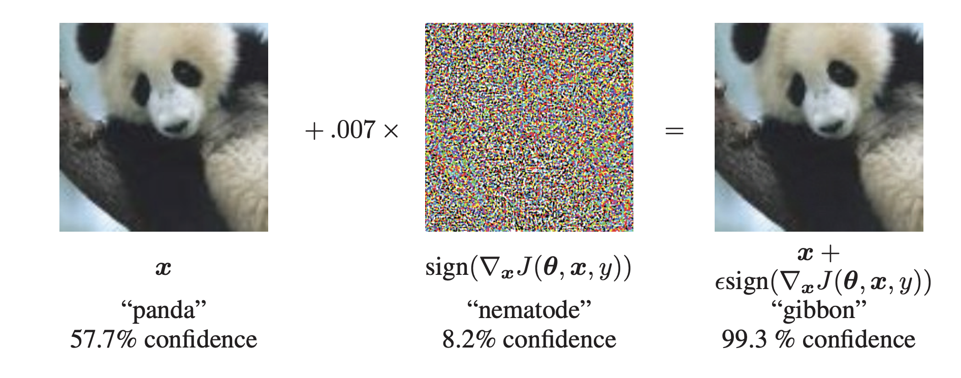
Figure 1: Example of an imperceptibly perturbed adversarial example (Goodfellow et al., 2015)

Figure 2: Example of an inconspicuously perturbed adversarial example (Evtimov et al., 2017)

3.1.2 Properties.

1. Imperceptibility: As described above, adversarial examples are typically designed to be such that their difference to the original sample is imperceptible to humans. As previously highlighted, this property can be relaxed to yield inconspicuous adversarial examples, where there is a visible change that does not alter the semantic features of the sample.

2. Cross-Model Transferability: Adversarial examples exhibit the property of cross-model transferability, whereby they can mislead different deep learning models trained on the same dataset (Szegedy et al., 2014; Goodfellow et al., 2015; Papernot et al., 2016).

3. Cross Training-Set Transferability: Adversarial examples can also be carefully designed to fool classifiers without directly modifying training samples. Models cannot guard against such examples by augmenting perturbed training samples.

Now that we have established what adversarial examples are, the question as to why deep learning models are particularly susceptible to these still remains. While this is still an ongoing research theme, studies have outlined several possible reasons for this vulnerability. In Arpit et al. (2017), the authors measure the memorization capacity of deep learning models and show that models with a greater degree of memorization are increasingly vulnerable to adversarial examples. In Jo and Bengio (2017), authors verify that convolutional architectures learn the surface statistical regularities of the training dataset, rather than abstract high-level representations. This provides a possible explanation for why adversarial examples may mislead the networks. Moveover, this study gives insight into the transferability property of adversarial examples: different models trained on the same dataset learn the same statistical regularities leading to them being fooled by the same adversarial example. Another line of reasoning as to why deep learning models are fallible is suggested in Ilyas et al. (2019), where the authors claim that models learn non-robust features during the training process.

3.2 Adversarial Attacks

3.2.1 Dichotomy of Adversarial Attacks.

Adversarial attacks are mainly categorized as white-box and black-box attacks. In the former, the attacker has full knowledge of the target model, e.g., with regards to its architecture, parameters, and gradient information. On the contrary, black-box attacks only have knowledge of the output of the target model. While in practice the black-box assumption is more realistic due to attackers not usually having full information on the target, white-box attacks are vital to consider to guard against the worst-case scenario.

Adversarial attacks can be alternatively characterized as targeted and non-targeted attacks. Here, targeting refers to specific manipulation of the output of the model. In targeted attacks, the attacker aims to design an adversarial example in a manner which causes the model to output a specific classification. Non-targeted attacks aim to elicit any form of misclassification.

3.2.2 White-Box Optimization-Based Attacks.

We first consider white-box optimization-based attacks, where the idea is to formulate an optimization problem involving the model’s loss function to directly find an adversary.

The Limited Memory Broyden-Fletcher-Goldfarb-Shanno (L-BFGS) (Szegedy et al., 2014) attack, is one of the earliest adversarial attack methods which was able to fool the then state-of-the-art AlexNet (Krizhevsky et al., 2012) and QuocNet architectures on image classification tasks. In this method of attack, the goal is to solve the optimization

$$\min_{x^{\prime}:f(x^{\prime})\neq f(x)}\|x-x^{\prime}\|_{2},$$ (5)

where as before $x$ is the non-adversarial sample and $f$ is the model. Solving this optimization essentially yields the sample $x^{\prime}$ of smallest perturbation that elicits misclassification. Due to the difficulty in solving the optimization (5), the authors of Szegedy et al. (2014) reformulated the problem into a box-constrained one:

$$\min_{x^{\prime}\in[0,1]^{d}}c\|x-x^{\prime}\|_{2}+\mathcal{L}(x^{\prime},t),$$ (6)

where $c>0$ is a scalar, $\mathcal{L}(\cdot,\cdot)$ represents the loss function of the target model (e.g., cross-entropy loss), $t$ is the target misclassification label, and the non-adversarial sample $x$ has been normalized to lie within the cube $[0,1]^{d}$. Problem (6) can be solved with the 2nd-order L-BFGS optimization algorithm giving the attack method its name. As the problem doesn’t have an explicit misclassification constraint, the solution is not guaranteed to be an adversarial example. The constant $c$ can be iteratively increased via line search until an adversary is obtained.

The L-BFGS attack (Szegedy et al., 2014) generates adversarial examples by optimizing over the loss between the model output and target class. An alternative formulation is to optimize over the similarity between the hidden representations of the perturbed sample and a target sample with a different class. The adversarial manipulation of deep representations (AMDR) method (Sabour et al., 2016) attempts to do exactly this. More formally, this method requires a non-adversarial subject $x$, a sample from another target class $x_{t}$, and a classifier $f$ such that $f(x)\neq f(x_{t})$. AMDR attempts to find an adversary $x^{\prime}$ that remains similar to $x$ but has an internal representation similar to $x_{t}$. The optimization is formulated as

$$\min_{x^{\prime}:\|x-x^{\prime}\|_{\infty}\leq\epsilon}\|f_{l}(x_{t})-f_{l}(x^{\prime})\|_{2},$$ (7)

where $f_{l}(\cdot)$ represents the intermediary output of $f$ at the $l^{\textrm{th}}$ layer. As opposed to the L-BFGS attack, the ADMR attack method requires a target sample $x_{t}$ (rather than a target label) and a particular hidden layer $l$. This method has been shown to fool architectures such as AlexNet (Krizhevsky et al., 2012), CaffeNet (Jia et al., 2014), and VGG variants (Chatfield et al., 2014) on the ImageNet (Deng et al., 2009; Russakovsky et al., 2014) and Places205 (Zhou et al., 2014) datasets.

Other notable white box optimization-based attack methods in this category include DeepFool (Moosavi-Dezfooli et al., 2016) and the Carlini-Wagner (Carlini and Wagner, 2017b) attacks. The former is based on finding the closest (nonlinear) decision boundary to a considered sample $x$ for a multi-class classifier. The minimal perturbation is then chosen to push the sample over the closest decision boundary. Carlini and Wagner (2017b) proposes a family of attacks that uses a similar notion of finding the smallest perturbation to a sample that yields the desired target classification. The authors develop different reformulations of the constraint that requires the perturbed sample $x^{\prime}$ to result in a model prediction of class $t$.

3.2.3 White-Box Gradient-Based Attacks.

The family of white-box gradient-based attack methods operate on the notion of finding a perturbation direction that increases the training loss function of the target model. While choosing a perturbation as such doesn’t guarantee misclassification, the target model’s classification confidence will decrease.

The fast gradient sign method (FGSM) (Goodfellow et al., 2015) is an early proponent of this idea. It computes the gradient of the target model’s loss function, and perturbs the instance $x$ according to the signs of the elements of the gradient:

$$x^{\prime}=x+\epsilon\cdot\textrm{sign}\left(\nabla_{x}\mathcal{L}(x,y)\right).$$ (8)

Here $\epsilon$ is a small constant scalar that determines the size of perturbation. Unlike white-box optimization-based methods where difficult optimization problems have to be solved to generate adversarial examples, in FGSM the main computational complexity lies in evaluating the gradient of the loss function. When considering deep networks, this can be efficiently computed using the back-propagation algorithm (Rumelhart et al., 1986). Moreover, since FGSM relies upon computing the gradient with respect to the model’s loss, it can be applied to fool any machine learning method. Variants of FGSM include fast gradient value method (Rozsa et al., 2016), basic iterative method (BIM) (Kurakin et al., 2016), momentum iterative FGSM (Dong et al., 2018), and R+FGSM (Tramèr et al., 2017). In (Huang et al., 2017), the authors demonstrate how adversarial examples generated by FGSM can be used to fool neural network parameterized policies in reinforcement learning. FGSM and its variants are single-step methods that assume linearity. Alternatively, the projected gradient descent (PGD) attack method (Madry et al., 2018) better explores the nonlinear landscape and thereby gives an improved chance of finding the worst-case adversarial example. PGD uses several iterations to find the perturbation that maximizes the loss of the model for a particular sample while keeping the perturbation small. In each iteration, this method takes a gradient step in the direction of the greatest loss and subsequently projects back onto an $\ell_{p}$-norm ball that constrains the perturbation.

3.2.4 Black-Box Attacks.

So far we have discussed white-box attacks that leverage knowledge of the inner workings of the target model. Black-box methods assume that attackers can only query the target model.

The substitute black-box attack (SBA) (Papernot et al., 2017) is one of the first proposed methods of this ilk. SBA generates a synthetic dataset labeled by the black-box model to then learn a substitute model as a means to imitate the target. Once the substitute model is trained, any of the white-box attacks discussed above can be used to generate adversarial examples. This method leverages the cross-model transferability property of adversarial examples. Boundary Attack (Brendel et al., 2018) is another black-box method used to find an adversarial example reminiscent of the sample $x$. In this method, an input $x^{\prime}$ sampled from another class is perturbed towards and along the decision boundary between the class of $x$ and its adjacent classes until the perceptual difference between $x$ and $x^{\prime}$ is sufficiently minimized. Chen et al. (2017) proposes zeroth order optimization (ZOO) attacks to directly estimate the gradients of the targeted deep network model in order to generate adversarial examples. In one-pixel attacks (Su et al., 2017), the target model is fooled by only changing a limited number of pixels of an image sample.

3.3 Adversarial Training Methods

So far, we have discussed a variety of methods developed to generate adversarial examples that have been shown to fool vulnerable target models. Adversarial training addresses this issue by making models robust towards worst-case adversarial examples. Therefore, the basic idea of adversarial training is to account for such worst-case perturbations by incorporating these during model training.

3.3.1 FGSM Adversarial Training.

FGSM Adversarial training (FGSM-AT) (Goodfellow et al., 2015) is one of the earliest adverserial training methods, which guards against adversarial examples by augmenting these to the training dataset during each training iteration. While in FGSM-AT the adversarial examples are generated using FGSM (Goodfellow et al., 2015), in practice this defense methodology can also be extended to other gradient-based attack methods such as BIM (Kurakin et al., 2017). The training objective for such adversarial training is of the form

$$\alpha\mathcal{L}(x,y)+(1-\alpha)\mathcal{L}(x^{\prime},y),$$ (9)

where $\alpha$ is a weighting parameter that trades off the importance of minimizing the loss with respect to the true sample $x$ and the adversarial sample $x^{\prime}$ generated by the attack method of choice. In practice $\alpha$ is often set to $0.5$ (Wiyatno et al., 2019). While FGSM-AT has demonstrated effectiveness in defending against single-step attacks on large datasets (Kurakin et al., 2017), models trained with this method have still shown to be vulnerable to multi-step attacks such as BIM or PGD. Kurakin et al. (2017) found that models trained on single-step attacks such as FGSM can suffer from the issue of label leakage. Here, it has been shown that the model trained on such single-step adversaries performs better on such adversaries than on clean data during evaluation. This suggests that examples generated by single-step adversarial attack methods may be too simple as the considered models are able to overfit on these (Wiyatno et al., 2019).

3.3.2 PGD Adversarial Training.

Projected gradient descent adversarial training (PGD-AT) was proposed by Madry et al. (2018) as a variant to adversarial training methods such as FGSM-AT (Goodfellow et al., 2015). PGD-AT is based on training against “worst-case” adversaries. The training objective is formulated as

$$\min_{\theta}\max_{x^{\prime}:\|x^{\prime}-x\|\leq\epsilon}\mathcal{L}(x^{\prime},y),$$ (10)

where we select model parameters $\theta$ to minimize the worst-case perturbation within a norm-ball of radius $\epsilon$ around sample $x$. This minimax problem is aligned with the robust optimization framework where the aim is to minimize the impact of the adversary’s worst-case moves. Note that PGD-AT is equivalent to setting $\alpha=0$ in objective (9) with $x^{\prime}$ being the worst-case adversarial example. Madry et al. (2018) show that adversaries generated using the PGD attack are indeed the worst-case adversarial examples. They demonstrate that even after restarting PGD from random starting points, the model’s loss plateaus to similar levels. The reason behind this is suggested to be numerous local maxima which are in turn quite similar to the global maxima (Madry et al., 2018). Therefore, the authors argue that training against PGD adversarial examples approximately solves the minimax problem (10). While PGD-AT has been shown to be particularly effective for large scale models (Madry et al., 2018), some drawbacks still exist. For one, it has been shown that PGD-AT significantly compromises the model’s accuracy on clean samples (Tsipras et al., 2019). Moreover, since the PGD attack is a multi-step method with a costly projection operation at each iteration, this method is subject to a higher computational cost compared to single-step adverarial training methods.

3.3.3 Ensemble Adversarial Training.

Another variant of adversarial training, proposed by Tramèr et al. (2018), is known as ensemble adversarial training. Here, a model is retrained using adversarial examples used to target other pre-trained models. It is suggested that the separation of generating the adversarial examples and the actual target model mitigates the overfitting issue seen in single-step adversarial training methods such as FGSM-AT. As the process of generating adversarial examples is independent of the model that is being trained, it is argued that ensemble adversarial training is more robust to black-box attacks compared to white-box adversarial training.

3.3.4 Convex Adversarial Training.

A more recent form of adversarial training is based on leveraging convex reformulations of the two-layer ReLU network training problem which are shown to have equivalent optimal values to the original non-convex problem (Pilanci and Ergen, 2020; Lacotte and Pilanci, 2020; Ergen and Pilanci, 2021). In (Bai et al., 2022a, b), the authors develop convex robust optimization problems for the adversarial training of two-layer ReLU networks, with a particular focus on the cases of hinge loss (for binary classification) and squared loss (for regression).

4 Robustness Certification

Over recent years, we have seen an “arms race” develop in the robustness literature; for every proposed defense, it seems as though a new attack is developed that is strong enough to defeat the defense (Carlini and Wagner, 2017a; Kurakin et al., 2017; Athalye et al., 2018; Uesato et al., 2018; Madry et al., 2018). This has led researchers to consider certified robustness, which is a mathematical proof that the model yields reliable outputs when subject to a certain threat model on the input. This threat model has been considered in both a stochastic framework, where the input uncertainty is random, as in Mangal et al. (2019); Weng et al. (2019); Webb et al. (2018); Fazlyab et al. (2019a); Anderson and Sojoudi (2022b), and an adversarial framework, where the input uncertainty is maliciously designed to fool the model. In this survey, we focus on the adversarial case, as it remains the standard threat model considered in the literature.

Certified defenses can roughly be categorized into methods based on satisfiability modulo theories (SMT), optimization- and relaxation-based bounds, and randomized smoothing. SMT-based methods such as Katz et al. (2017); Amir et al. (2021) comprise some of the earliest robustness certificates, but, as they are combinatorial in nature, the field has turned towards more tractable bounding techniques. These tractable certificates are the ones we focus on going forward.

4.1 Optimization-Based Methods

Consider a general neural network $f\colon\mathbf{R}^{d}\to\mathbf{R}^{n}$. The threat model considered in optimization-based methods is one in which the input to the neural network is contained in some input uncertainty set $\mathcal{X}\subseteq\mathbf{R}^{d}$, but is otherwise unknown. It is common in the literature to assume that $\mathcal{X}$ is either a compact convex polytope or that $\mathcal{X}=\{x\in\mathbf{R}^{d}:\|x-\overline{x}\|_{p}\leq r\}$ for some nominal input $\overline{x}\in\mathbf{R}^{d}$ and some attack radius $r>0$. The goal of an adversary is to find an input $x^{\star}\in\mathcal{X}$ to achieve the worst-case output $f(x^{\star})$, e.g., to cause misclassification in a classification task. On the other hand, the goal of the defender is to certify that all outputs $f(x)$ corresponding to inputs $x\in\mathcal{X}$ are “safe” in some sense. Safety can generally be modeled by a subset $\mathcal{S}$ of the output space $\mathbf{R}^{n}$, which is commonly taken to be a (possibly unbounded) polytope. For example, suppose that $f$ is an $n$-class classifier and that $f(x)_{i}$ represents the confidence associated to class $i$, so that the class assigned to an input $x$ is given by $\operatorname*{arg\,max}_{i\in\{1,\dots,n\}}f(x)_{i}$. Then, if $\overline{x}$ is classified into class $i^{*}$ and we seek to certify that adversarial perturbations of $\overline{x}$ are not misclassified, then the problem amounts to showing that $f(\mathcal{X})\subseteq\mathcal{S}$ with the safe set being the half-space $\mathcal{S}=\{y\in\mathbf{R}^{n}:c^{\top}y\geq 0\}$ with $c=e_{i^{*}}-e_{i}$. We will assume that the safe set is a half-space going forward.

With these preliminaries in place, we may now formally define the robustness certification problem as the following optimization problem:

$$p^{\star}=\inf_{x\in\mathcal{X}}c^{\top}f(x).$$ (11)

If the optimal value $p^{\star}$ for (11) is nonnegative, then $c^{\top}f(x)\geq 0$ for all $x\in\mathcal{X}$, implying that $f(\mathcal{X})\subseteq\mathcal{S}$, so all inputs are certified to yield safe outputs. Notice though, that most neural networks $f$ are nonconvex functions, making (11) a nonconvex optimization problem even for convex $\mathcal{X}$. In fact, the certification problem (11) for neural networks is proven to be NP-hard (Katz et al., 2017; Weng et al., 2018). Thus, most works make the certification procedure more tractable by either developing convex relaxations of (11), or directly bounding and analyzing $f$ over the set $\mathcal{X}$. Notice that, if $\hat{f}(\mathcal{X})\supseteq f(\mathcal{X})$ and $p^{\prime}=\inf_{y\in\hat{f}(\mathcal{X})}c^{\top}y$ is a convex relaxation of $p^{\star}$, then $p^{\prime}\leq p^{\star}$, so to prove the robustness of $f$ with respect to the threat model $\mathcal{X}$ it suffices to show that $p^{\prime}\geq 0$. This approach to certification is illustrated graphically in Figure 3. We now discuss such methods in more detail.

Figure 3: Certifying the safety of a convex outer-approximation $\hat{f}(\mathcal{X})$ of the nonconvex output set $f(\mathcal{X})$ is sufficient to prove robustness. If the convex approximation is too loose, it may enter the unsafe region and fail to certify (Anderson et al., 2021)

4.1.1 Linear Programming.

In the context of $\operatorname{ReLU}$ neural networks, Wong and Kolter (2018) proposes to relax the nonlinear $\operatorname{ReLU}$ equality constraints in (11) to their convex upper envelop. This is accomplished by introducing three linear inequalities associated to every neuron in the network. The approach is simple, scalable, and capable of being used to learn provably robust networks, but in general the feasible set grows crudely with the depth of the network, turning researchers to consider more sophisticated relaxations. Subsequent works consider fast linear bounds on $\operatorname{ReLU}$ activations (Weng et al., 2018), generalizing the linear bounding technique past $\operatorname{ReLU}$ activations (Zhang et al., 2018; Dvijotham et al., 2018; Wong et al., 2018), and combining linear bounds with symbolic interval analysis to attain tighter relaxations (Wang et al., 2018). Salman et al. (2019b) goes on to unify these linear programming-based methods and show that they suffer from a so-called “convex relaxation barrier” preventing tight certification under this framework. The paper Tjandraatmadja et al. (2020) proposed to overcome this barrier by using a tightened, joint linear relaxation of $\operatorname{ReLU}$ networks instead of the prior neuron-wise relaxations.

Gowal et al. (2018) considers using interval bounds on each layer’s activation values to obtain a bound on the optimal value of (11), and incorporate this efficient procedure into the training process to learn certifiably robust networks. Other works such as Hein and Andriushchenko (2017); Ruan et al. (2018); Fazlyab et al. (2019b) derive bounds and estimates on the Lipschitz constant of a neural network, which is then able to be used to assess the network’s robustness.

4.1.2 Semidefinite Programming.

Since the feasible set of linear programming relaxations grows crudely as the size of the network grows, researchers have considered nonlinear convex relaxations in order to tighten the certification. The authors of Raghunathan et al. (2018) reformulate (11) for $\operatorname{ReLU}$ networks as an optimization over a lifted positive semidefinite matrix variable with a rank-1 constraint. By dropping the rank constraint, they arrive at a semidefinite program, which is found to outperform linear programming relaxations—especially for deep networks—increasing the percentage of certified MNIST examples at an $\ell_{\infty}$-attack radius of $r=0.1$ by over 80% for networks learned via PGD adversarial training. The work Zhang (2020) theoretically showed that this semidefinite relaxation is tight for a single hidden layer under mild technical assumptions. In Fazlyab et al. (2020), quadratic constraints are used to describe a neural network’s activation function, and the S-procedure is then used to arrive at a tightened semidefinite relaxation. Although these semidefinite relaxations yield good bounds on robustness, they are not generally applicable to large-scale settings.

4.1.3 Partitioned and Mixed-Integer Programming.

In order to reach a middle ground attaining both the computational tractability of simple linear programming relaxations and the tightness of more sophisticated relaxations, a line of works has been developed that make use of partitioning schemes and mixed-integer optimization formulations. For example, Tjeng et al. (2017) reformulates the certification problem (11) for $\operatorname{ReLU}$ networks into a mixed-integer linear program that scales up to networks of $100,000$ neurons, and is able to solve for $p^{\star}$ exactly. The paper Bunel et al. (2018) builds on this formulation and proposes an efficient branch-and-bound algorithm for estimating the optimal value.

Related to the mixed-integer formulation is the partitioned programming approach, wherein the input set $\mathcal{X}$ is partitioned into smaller subsets, and the optimization (11) is solved over each subset individually to arrive at an overall global bound on $p^{\star}$. The partitioning is effective since convex relaxations tend to become tighter as the feasible set of the optimization becomes smaller. An example of this approach is Xiang and Johnson (2018), where the input uncertainty set is partitioned into hyperrectangles, leading to tightened certification of networks with general activation functions. The work Rubies-Royo et al. (2019) uses Lagrangian duality to motivate a partition of box-shaped input uncertainty sets along coordinate axes. In a similar vein, Everett et al. (2020) theoretically characterizes the reduction in volume of the resulting outer-approximation of $f(\mathcal{X})$ upon using axis-aligned partitioning in the input space. In Anderson et al. (2020), the authors upper-bound the worst-case relaxation error induced by the linear programming approach of Wong and Kolter (2018), and then derive a closed-form expression for the optimal partition of $\mathcal{X}$ that minimizes this worst-case error. Ma and Sojoudi (2021) propose a partitioning scheme that sequentially reduces the relaxation error of the semidefinite programming approach and characterizes its effect on the feasible set geometry. The work Wang et al. (2021b) develops a parallelizable bound propagation method that optimizes over partitioning parameters leading to state-of-the-art certification results, outperforming semidefinite relaxations on MNIST and CIFAR-10 benchmarks in terms of both time and certified accuracy, and winning the 2021 Verification of Neural Networks Competition (Bak et al., 2021).

4.2 Randomized Smoothing

Randomized smoothing, popularized in Lecuyer et al. (2019); Li et al. (2019); Cohen et al. (2019), is a probabilistic method to robustify a classifier $f\colon\mathbf{R}^{d}\to\{1,2,\dots,n\}$ with deterministic robustness guarantees. Formally, we consider a hard-classifier $f(x)\in\operatorname*{arg\,max}_{i\in\{1,2,\dots,n\}}g_{i}(x)$ for some associated soft-classifier $g\colon\mathbf{R}^{d}\to\mathbf{R}^{n}$. The majority of works on randomized smoothing assume that the image of $g$ is the probability simplex in $[0,1]^{n}$—a realistic assumption that simplifies the analyses. Now, letting $\mu$ denote some probability distribution on the input space $\mathbf{R}^{d}$, randomized smoothing proposes to replace the classifier $f$ by the following “smoothed classifier”:

$$f^{\mu}(x)\in\operatorname*{arg\,max}_{i\in\{1,2,\dots,n\}}g_{i}^{\mu}(x),\quad g_{i}^{\mu}(x)=\mathbf{E}_{\epsilon\sim\mu}g(x+\epsilon).$$

Intuitively, randomized smoothing intentionally corrupts an input $x$ by additive random noise, feeds that through the base classifier, and uses the average prediction of these noisy inputs as the actual prediction for $x$. The idea behind this process is to “average out” any potential dangerous, yet unlikely adversarial perturbations, in effect robustifying the classification scheme. This is graphically illustrated in Figure 4.

Figure 4: Randomized smoothing smooths out jagged regions of the base classifier decision boundary (left) to certifiably increase the robust radius around inputs (right) (Anderson et al., 2022)

The most common distribution $\mu$ to use is an unbiased symmetric Gaussian, i.e., $N(0,\sigma^{2}I_{d})$ for some user-prescribed variance $\sigma^{2}$. We first describe this setup, and then move on to discuss variants and on-going work to generalize the smoothing framework.

4.2.1 Symmetric Gaussian Smoothing.

Symmetric Gaussian smoothing, where $\mu=N(0,\sigma^{2}I_{d})$, is the most common form of randomized smoothing. This is the method introduced in Lecuyer et al. (2019); Li et al. (2019), and popularized in Cohen et al. (2019) with provably tight robustness guarantee, which we recall in the following theorem.

Theorem 1 (Cohen et al., 2019; Zhai et al., 2020)

Let $\sigma^{2}$ be a positive real number and consider $\mu=N(0,\sigma^{2}I_{d})$. Consider a point $x\in\mathbf{R}^{d}$ and let $y=f^{\mu}(x)\in\operatorname*{arg\,max}_{i\in\{1,\dots,n\}}g^{\mu}_{i}(x)$ and $y^{\prime}\in\operatorname*{arg\,max}_{i\in\{1,\dots,n\}\setminus\{y\}}g^{\mu}_{i}(x)$. Then $f^{\mu}(x+\delta)=y$ for all $\delta\in\mathbf{R}^{d}$ such that

$$\|\delta\|_{2}\leq r^{\mu}(x)\coloneqq\frac{\sigma}{2}\left(\Phi^{-1}(g^{\mu}_{y}(x))-\Phi^{-1}(g^{\mu}_{y^{\prime}}(x))\right).$$

Theorem 1 says that any attack of $\ell_{2}$-norm less than $r^{\mu}(x)$ cannot change the prediction of the nominal input $x$. This certified robustness guarantee enables the use of smoothed models in safety-critical systems with confidence in their reliability, e.g., policies in reinforcement learning or neural network-based controllers (Wu et al., 2021; Kumar et al., 2021). Due to its efficient statistical nature, randomized smoothing is able to scale to extremely large settings, even allowing for the certification of ImageNet models (Cohen et al., 2019), which had previously been intractable for non-smoothing-based certification methods.

Follow-up works attempt to increase the size of the certified region using a variety of different approaches. For example, Salman et al. (2019a) incorporates adversarial training into the Gaussian smoothing scheme to obtain state-of-the-art $\ell_{2}$-norm certified radii. On the other hand, Zhai et al. (2020) develops a tractable method to maximize the certified radius over the smoothing variance $\sigma^{2}$. The authors of Zhang et al. (2020) look at optimizing the base classifier in order to achieve maximal certified radii, and their experiments show a notable increase in certified robust accuracy over the baseline Cohen et al. (2019). More recently, the authors of Pfrommer et al. (2022) incorporated dimensionality reduction of the neural network’s input in order to perform Gaussian smoothing in a lower-dimensional space. This in effect projects-out perturbations that are normal to the natural data manifold, enlarging the certified region along such directions in the input space.

There has also been a line of works demonstrating negative results for randomized smoothing. For example, the works Tsipras et al. (2019); Krishnan et al. (2020); Yang et al. (2020b); Gao et al. (2020) all point to an inherent accuracy-robustness tradeoff for smoothed models. That is, as $\sigma^{2}$ increases, the model becomes smoother, and hence its regions of constant classification become larger, but accuracy on clean test samples ends up suffering once $\sigma^{2}$ becomes too large. Another intriguing negative result is the “shrinking phenomenon” discovered in Mohapatra et al. (2021), where, as $\sigma^{2}$ increases, bounded decision regions and those contained within a narrow cone tend to shrink, causing imbalances in classwise accuracies.

4.2.2 Alternative Smoothing Distributions.

As symmetric Gaussian smoothing only yields certified regions taking the form of an isotropic $\ell_{2}$-ball, researchers have worked on generalizing randomized smoothing to certify alternatively shaped regions. The work Teng et al. (2020) uses a Laplacian smoothing distribution to certify $\ell_{1}$-norm balls, Levine and Feizi (2020) certifies against attacks defined in terms of the Wasserstein distance, Lee et al. (2019) uses discrete distributions to certify against cardinality-constrained “$\ell_{0}$”-attacks, and Yang et al. (2020a) characterize the optimal smoothing distributions corresponding to $\ell_{1}$-, $\ell_{2}$-, and $\ell_{\infty}$-attacks. The authors of Erdemir et al. (2021) extend randomized smoothing to an asymmetric variant in order to certify anisotropic regions of the input space.

4.2.3 Input-Dependent Smoothing.

Since inputs close to the base classifier decision boundary may require small smoothing variance to maintain clean accuracy, yet inputs far from the decision boundary may permit large variance so as to increase their corresponding certified radii, a recent push to allow for input-dependent smoothing distributions has been made. In particular, the smoothing distribution $\mu$ is replaced by $\mu(x)$, which is a probability distribution that may differ between inputs $x$.

In order to derive mathematically valid robustness certificates, additional assumptions on the map $x\mapsto\mu(x)$ must be made. For example, the works Alfarra et al. (2020); Wang et al. (2021a) choose $\mu(x)$ to be a normal distribution such that the variance is optimized for particular data points locally in the vicinity of $x$. However, this approach amounts to a classifier that is dependent on the order of incoming inputs for which the variances are optimized, in effect introducing another uncertainty into the classification scheme as well as a vulnerability that an adversary may exploit. The work Eiras et al. (2021) generalizes this approach to certify anisotropic ellipsoids, choosing the Gaussian covariance to maximize the volume of the ellipsoids in a pointwise fashion.

In Súkeník et al. (2021), it is shown that, in general, input-dependent randomized smoothing suffers from the curse of dimensionality. The authors propose a parameterization of the smoothing scheme that avoids the order-dependence of the classifier from the prior works, but without notable improvement in the certified accuracies over conventional input-independent randomized smoothing. The authors of Anderson and Sojoudi (2022a) argue that effective randomized smoothing schemes should be designed with the underlying data distribution in mind, and they show that in order to achieve this the smoothing distribution must necessarily be input-dependent and have a nonzero mean. Accordingly, they develop an input-dependent smoothing scheme for binary classifiers that is optimal up to a first-order approximation of the base classifier. Along similar lines, Anderson et al. (2022) formulates the optimal randomized smoothing problem as the optimization over general (not necessarily Gaussian) distribution-valued maps $x\mapsto\mu(x)$ subject to constraints on their Lipschitz continuity. The Lipschitz condition is utilized in order to derive mathematically valid certified radii for the resulting model. They show that the optimal distribution can be approximated by a semi-infinite linear program, and prove that the resulting problem satisfies nontrivial strong duality, allowing for more tractable computations. Although there has been much research developed surrounding randomized smoothing and its variants, the problem of exactly optimizing the smoothing distribution in a manner scalable to large datasets such as ImageNet appears to remain open.

5 Conclusions and Directions for Future Research

While there have been great strides in recent years on finding new methods to generate and defend against adversarial attacks, the fundamental question regarding why deep architectures are vulnerable to such adversarial examples still remains open. A unified theory explaining the vulnerability as well as properties such as cross-model transferability will in turn provide valuable insight into effective training methods that are robust to a variety of attacks. Another direction of future research relates to standardizing robustness evaluation across different attacks. Currently, defense approaches claim that they can guard against certain attacks while failing against others. A standardized evaluation framework will enable a fair judgement on the defense efficacy of robust training methods for different attacks.

In the realm of certification, it appears to remain an open problem to derive optimization-based methods for general (non-$\operatorname{ReLU}$) activations that are tight enough to yield meaningful guarantees while being computationally tractable enough to scale to large benchmarks like ImageNet. The problem of optimizing input-dependent randomized smoothing schemes is a promising direction for certifiably robustifying classifiers in the large-scale setting, but more work must be done in order to tractably solve for such distributions without resorting to heuristics such as locally-constant input-to-distribution maps.

References

- Alfarra et al. (2020) Alfarra, M., Bibi, A., Torr, P.H., and Ghanem, B. (2020). Data dependent randomized smoothing. arXiv preprint arXiv:2012.04351.
- Amir et al. (2021) Amir, G., Wu, H., Barrett, C., and Katz, G. (2021). An smt-based approach for verifying binarized neural networks. In International Conference on Tools and Algorithms for the Construction and Analysis of Systems, 203–222. Springer.
- Anderson et al. (2020) Anderson, B.G., Ma, Z., Li, J., and Sojoudi, S. (2020). Tightened convex relaxations for neural network robustness certification. In 2020 59th IEEE Conference on Decision and Control (CDC), 2190–2197. IEEE.
- Anderson et al. (2021) Anderson, B.G., Ma, Z., Li, J., and Sojoudi, S. (2021). Partition-based convex relaxations for certifying the robustness of ReLU neural networks. arXiv preprint arXiv:2101.09306.
- Anderson et al. (2022) Anderson, B.G., Pfrommer, S., and Sojoudi, S. (2022). Towards optimal randomized smoothing: A semi-infinite linear programming approach. In ICML Workshop on Formal Verification of Machine Learning (WFVML).
- Anderson and Sojoudi (2022a) Anderson, B.G. and Sojoudi, S. (2022a). Certified robustness via locally biased randomized smoothing. In Learning for Dynamics and Control. PMLR.
- Anderson and Sojoudi (2022b) Anderson, B.G. and Sojoudi, S. (2022b). Data-driven certification of neural networks with random input noise. IEEE Transactions on Control of Network Systems.
- Arpit et al. (2017) Arpit, D., Jastrzundefinedbski, S., Ballas, N., Krueger, D., Bengio, E., Kanwal, M.S., Maharaj, T., Fischer, A., Courville, A., Bengio, Y., and Lacoste-Julien, S. (2017). A closer look at memorization in deep networks. In Proceedings of the 34th International Conference on Machine Learning. JMLR.org.
- Athalye et al. (2018) Athalye, A., Carlini, N., and Wagner, D. (2018). Obfuscated gradients give a false sense of security: Circumventing defenses to adversarial examples. In International Conference on Machine Learning. PMLR.
- Bai et al. (2022a) Bai, Y., Gautam, T., Gai, Y., and Sojoudi, S. (2022a). Practical convex formulation of robust one-hidden-layer neural network training. In 2022 American Control Conference (ACC).
- Bai et al. (2022b) Bai, Y., Gautam, T., and Sojoudi, S. (2022b). Efficient global optimization of two-layer ReLU networks: Quadratic-time algorithms and adversarial training. arXiv preprint arXiv:2201.01965.
- Bak et al. (2021) Bak, S., Liu, C., and Johnson, T. (2021). The second international verification of neural networks competition (vnn-comp 2021): Summary and results. arXiv preprint arXiv:2109.00498.
- Ben-Tal et al. (2009) Ben-Tal, A., El Ghaoui, L., and Nemirovski, A. (2009). Robust Optimization. Princeton Series in Applied Mathematics. Princeton University Press.
- Ben-Tal and Nemirovski (2000) Ben-Tal, A. and Nemirovski, A. (2000). Robust solutions of linear programming problems contaminated with uncertain data. Mathematical Programming, 88, 411–424. 10.1007/PL00011380.
- Ben-Tal and Nemirovski (2002) Ben-Tal, A. and Nemirovski, A. (2002). Robust optimization-methodology and applications. Math. Program., 92, 453–480. 10.1007/s101070100286.
- Bertsimas et al. (2011) Bertsimas, D., Brown, D.B., and Caramanis, C. (2011). Theory and applications of robust optimization. SIAM review, 53(3), 464–501.
- Bertsimas et al. (2018) Bertsimas, D., Gupta, V., and Kallus, N. (2018). Data-driven robust optimization. Mathematical Programming, 167(2), 235–292.
- Bertsimas and Sim (2004) Bertsimas, D. and Sim, M. (2004). The price of robustness. Operations Research, 52, 35–53. 10.1287/opre.1030.0065.
- Biggio et al. (2013) Biggio, B., Corona, I., Maiorca, D., Nelson, B., Šrndić, N., Laskov, P., Giacinto, G., and Roli, F. (2013). Evasion attacks against machine learning at test time. In Joint European conference on machine learning and knowledge discovery in databases. Springer.
- Blanchet et al. (2016) Blanchet, J., Kang, Y., and Murthy, K. (2016). Robust wasserstein profile inference and applications to machine learning. Journal of Applied Probability, 56. 10.1017/jpr.2019.49.
- Boyd and Vandenberghe (2004) Boyd, S. and Vandenberghe, L. (2004). Convex optimization. Cambridge university press.
- Brendel et al. (2018) Brendel, W., Rauber, J., and Bethge, M. (2018). Decision-based adversarial attacks: Reliable attacks against black-box machine learning models. ArXiv, abs/1712.04248.
- Brown et al. (2017) Brown, T.B., Mané, D., Roy, A., Abadi, M., and Gilmer, J. (2017). Adversarial patch. arXiv preprint arXiv:1712.09665.
- Bunel et al. (2018) Bunel, R.R., Turkaslan, I., Torr, P., Kohli, P., and Mudigonda, P.K. (2018). A unified view of piecewise linear neural network verification. Advances in Neural Information Processing Systems.
- Carlini and Wagner (2017a) Carlini, N. and Wagner, D. (2017a). Adversarial examples are not easily detected: Bypassing ten detection methods. In Proceedings of the 10th ACM Workshop on Artificial Intelligence and Security.
- Carlini and Wagner (2017b) Carlini, N. and Wagner, D.A. (2017b). Towards evaluating the robustness of neural networks. 2017 IEEE Symposium on Security and Privacy (SP).
- Chatfield et al. (2014) Chatfield, K., Simonyan, K., Vedaldi, A., and Zisserman, A. (2014). Return of the devil in the details: Delving deep into convolutional nets. arXiv preprint arXiv:1405.3531.
- Chen et al. (2017) Chen, P.Y., Zhang, H., Sharma, Y., Yi, J., and Hsieh, C.J. (2017). Zoo: Zeroth order optimization based black-box attacks to deep neural networks without training substitute models. In Proceedings of the 10th ACM Workshop on Artificial Intelligence and Security.
- Cohen et al. (2019) Cohen, J., Rosenfeld, E., and Kolter, Z. (2019). Certified adversarial robustness via randomized smoothing. In International Conference on Machine Learning. PMLR.
- Deng et al. (2009) Deng, J., Dong, W., Socher, R., Li, L.J., Li, K., and Fei-Fei, L. (2009). Imagenet: A large-scale hierarchical image database. In 2009 IEEE Conference on Computer Vision and Pattern Recognition.
- Dong et al. (2018) Dong, Y., Liao, F., Pang, T., Su, H., Zhu, J., Hu, X., and Li, J. (2018). Boosting adversarial attacks with momentum. In 2018 IEEE/CVF Conference on Computer Vision and Pattern Recognition.
- Duchi et al. (2016) Duchi, J., Glynn, P., and Namkoong, H. (2016). Statistics of robust optimization: A generalized empirical likelihood approach. arXiv preprint arXiv:1610.03425.
- Dvijotham et al. (2018) Dvijotham, K., Stanforth, R., Gowal, S., Mann, T.A., and Kohli, P. (2018). A dual approach to scalable verification of deep networks. In UAI.
- Eiras et al. (2021) Eiras, F., Alfarra, M., Kumar, M.P., Torr, P.H., Dokania, P.K., Ghanem, B., and Bibi, A. (2021). ANCER: Anisotropic certification via sample-wise volume maximization. arXiv preprint arXiv:2107.04570.
- El Ghaoui and Lebret (1997) El Ghaoui, L. and Lebret, H. (1997). Robust solutions to least-squares problems with uncertain data. SIAM Journal on Matrix Analysis and Applications, 18, 1035–1064.
- Erdemir et al. (2021) Erdemir, E., Bickford, J., Melis, L., and Aydore, S. (2021). Adversarial robustness with non-uniform perturbations. Advances in Neural Information Processing Systems.
- Ergen and Pilanci (2021) Ergen, T. and Pilanci, M. (2021). Implicit convex regularizers of CNN architectures: Convex optimization of two- and three-layer networks in polynomial time. In International Conference on Learning Representations.
- Everett et al. (2020) Everett, M., Habibi, G., and How, J.P. (2020). Robustness analysis of neural networks via efficient partitioning: Theory and applications in control systems. arXiv preprint arXiv:2010.00540.
- Evtimov et al. (2017) Evtimov, I., Eykholt, K., Fernandes, E., Kohno, T., Li, B., Prakash, A., Rahmati, A., and Song, D. (2017). Robust physical-world attacks on machine learning models. arXiv preprint arXiv:1707.08945.
- Fazlyab et al. (2019a) Fazlyab, M., Morari, M., and Pappas, G.J. (2019a). Probabilistic verification and reachability analysis of neural networks via semidefinite programming. In 2019 IEEE 58th Conference on Decision and Control (CDC), 2726–2731. IEEE.
- Fazlyab et al. (2020) Fazlyab, M., Morari, M., and Pappas, G.J. (2020). Safety verification and robustness analysis of neural networks via quadratic constraints and semidefinite programming. IEEE Transactions on Automatic Control.
- Fazlyab et al. (2019b) Fazlyab, M., Robey, A., Hassani, H., Morari, M., and Pappas, G. (2019b). Efficient and accurate estimation of lipschitz constants for deep neural networks. Advances in Neural Information Processing Systems.
- Gao et al. (2020) Gao, Y., Rosenberg, H., Fawaz, K., Jha, S., and Hsu, J. (2020). Analyzing accuracy loss in randomized smoothing defenses. arXiv preprint arXiv:2003.01595.
- Goodfellow et al. (2016) Goodfellow, I., Bengio, Y., and Courville, A. (2016). Deep Learning. MIT Press.
- Goodfellow et al. (2015) Goodfellow, I.J., Shlens, J., and Szegedy, C. (2015). Explaining and harnessing adversarial examples.
- Gowal et al. (2018) Gowal, S., Dvijotham, K., Stanforth, R., Bunel, R., Qin, C., Uesato, J., Arandjelovic, R., Mann, T., and Kohli, P. (2018). On the effectiveness of interval bound propagation for training verifiably robust models. arXiv preprint arXiv:1810.12715.
- Hein and Andriushchenko (2017) Hein, M. and Andriushchenko, M. (2017). Formal guarantees on the robustness of a classifier against adversarial manipulation. Advances in neural information processing systems.
- Huang et al. (2017) Huang, S.H., Papernot, N., Goodfellow, I.J., Duan, Y., and Abbeel, P. (2017). Adversarial attacks on neural network policies. ArXiv, abs/1702.02284.
- Ilyas et al. (2019) Ilyas, A., Santurkar, S., Tsipras, D., Engstrom, L., Tran, B., and Madry, A. (2019). Adversarial examples are not bugs, they are features. In H. Wallach, H. Larochelle, A. Beygelzimer, F. d'Alché-Buc, E. Fox, and R. Garnett (eds.), Advances in Neural Information Processing Systems.
- Jia et al. (2014) Jia, Y., Shelhamer, E., Donahue, J., Karayev, S., Long, J., Girshick, R., Guadarrama, S., and Darrell, T. (2014). Caffe: Convolutional architecture for fast feature embedding. MM 2014 - Proceedings of the 2014 ACM Conference on Multimedia.
- Jo and Bengio (2017) Jo, J. and Bengio, Y. (2017). Measuring the tendency of cnns to learn surface statistical regularities. ArXiv, abs/1711.11561.
- Katz et al. (2017) Katz, G., Barrett, C., Dill, D.L., Julian, K., and Kochenderfer, M.J. (2017). Reluplex: An efficient smt solver for verifying deep neural networks. In International Conference on Computer Aided Verification. Springer.
- Krishnan et al. (2020) Krishnan, V., Makdah, A., AlRahman, A., and Pasqualetti, F. (2020). Lipschitz bounds and provably robust training by laplacian smoothing. Advances in Neural Information Processing Systems.
- Krizhevsky et al. (2012) Krizhevsky, A., Sutskever, I., and Hinton, G.E. (2012). Imagenet classification with deep convolutional neural networks. Communications of the ACM.
- Kumar et al. (2021) Kumar, A., Levine, A., and Feizi, S. (2021). Policy smoothing for provably robust reinforcement learning. arXiv preprint arXiv:2106.11420.
- Kurakin et al. (2016) Kurakin, A., Goodfellow, I., and Bengio, S. (2016). Adversarial machine learning at scale. arXiv preprint arXiv:1611.01236.
- Kurakin et al. (2017) Kurakin, A., Goodfellow, I., and Bengio, S. (2017). Adversarial machine learning at scale.
- Lacotte and Pilanci (2020) Lacotte, J. and Pilanci, M. (2020). All local minima are global for two-layer ReLU neural networks: The hidden convex optimization landscape.
- Lam (2013) Lam, H. (2013). Robust sensitivity analysis for stochastic systems. Mathematics of Operations Research, 41. 10.1287/moor.2015.0776.
- Lecuyer et al. (2019) Lecuyer, M., Atlidakis, V., Geambasu, R., Hsu, D., and Jana, S. (2019). Certified robustness to adversarial examples with differential privacy. In 2019 IEEE Symposium on Security and Privacy (SP). IEEE.
- Lee et al. (2019) Lee, G.H., Yuan, Y., Chang, S., and Jaakkola, T. (2019). Tight certificates of adversarial robustness for randomly smoothed classifiers. Advances in Neural Information Processing Systems.
- Levine and Feizi (2020) Levine, A. and Feizi, S. (2020). Wasserstein smoothing: Certified robustness against wasserstein adversarial attacks. In International Conference on Artificial Intelligence and Statistics. PMLR.
- Li et al. (2019) Li, B., Chen, C., Wang, W., and Carin, L. (2019). Certified adversarial robustness with additive noise. Advances in Neural Information Processing Systems.
- Ma and Sojoudi (2021) Ma, Z. and Sojoudi, S. (2021). A sequential framework towards an exact SDP verification of neural networks. In 2021 IEEE 8th International Conference on Data Science and Advanced Analytics (DSAA).
- Madry et al. (2018) Madry, A., Makelov, A., Schmidt, L., Tsipras, D., and Vladu, A. (2018). Towards deep learning models resistant to adversarial attacks. In International Conference on Learning Representations.
- Mangal et al. (2019) Mangal, R., Nori, A.V., and Orso, A. (2019). Robustness of neural networks: A probabilistic and practical approach. In 2019 IEEE/ACM 41st International Conference on Software Engineering: New Ideas and Emerging Results (ICSE-NIER), 93–96. IEEE.
- Mohajerin Esfahani and Kuhn (2018) Mohajerin Esfahani, P. and Kuhn, D. (2018). Data-driven distributionally robust optimization using the Wasserstein metric: Performance guarantees and tractable reformulations. Mathematical Programming, 171(1), 115–166.
- Mohapatra et al. (2021) Mohapatra, J., Ko, C.Y., Weng, L., Chen, P.Y., Liu, S., and Daniel, L. (2021). Hidden cost of randomized smoothing. In International Conference on Artificial Intelligence and Statistics. PMLR.
- Moosavi-Dezfooli et al. (2016) Moosavi-Dezfooli, S.M., Fawzi, A., and Frossard, P. (2016). DeepFool: A simple and accurate method to fool deep neural networks. In 2016 IEEE Conference on Computer Vision and Pattern Recognition (CVPR).
- Papernot et al. (2016) Papernot, N., McDaniel, P., and Goodfellow, I. (2016). Transferability in machine learning: from phenomena to black-box attacks using adversarial samples. arXiv preprint arXiv:1605.07277.
- Papernot et al. (2017) Papernot, N., McDaniel, P., Goodfellow, I., Jha, S., Celik, Z.B., and Swami, A. (2017). Practical black-box attacks against machine learning. In Proceedings of the 2017 ACM on Asia Conference on Computer and Communications Security.
- Perdomo et al. (2020) Perdomo, J., Zrnic, T., Mendler-Dünner, C., and Hardt, M. (2020). Performative prediction. In International Conference on Machine Learning. PMLR.
-
Pfrommer et al. (2022)
Pfrommer, S., Anderson, B.G., and Sojoudi, S. (2022).
Projected randomized smoothing for certified adversarial robustness.
Preprint.
URL https://brendon-anderson.github.io/files/
publications/pfrommer2022projected.pdf. - Pilanci and Ergen (2020) Pilanci, M. and Ergen, T. (2020). Neural networks are convex regularizers: Exact polynomial-time convex optimization formulations for two-layer networks. In International Conference on Machine Learning.
- Raghunathan et al. (2018) Raghunathan, A., Steinhardt, J., and Liang, P.S. (2018). Semidefinite relaxations for certifying robustness to adversarial examples. Advances in Neural Information Processing Systems.
- Ross et al. (2011) Ross, S., Gordon, G., and Bagnell, D. (2011). A reduction of imitation learning and structured prediction to no-regret online learning. In Proceedings of the Fourteenth International Conference on Artificial Intelligence and Statistics. JMLR Workshop and Conference Proceedings.
- Rozsa et al. (2016) Rozsa, A., Rudd, E.M., and Boult, T.E. (2016). Adversarial diversity and hard positive generation. In 2016 IEEE Conference on Computer Vision and Pattern Recognition Workshops (CVPRW).
- Ruan et al. (2018) Ruan, W., Huang, X., and Kwiatkowska, M. (2018). Reachability analysis of deep neural networks with provable guarantees. arXiv preprint arXiv:1805.02242.
- Rubies-Royo et al. (2019) Rubies-Royo, V., Calandra, R., Stipanovic, D.M., and Tomlin, C. (2019). Fast neural network verification via shadow prices. arXiv preprint arXiv:1902.07247.
- Rumelhart et al. (1986) Rumelhart, D.E., Hinton, G.E., and Williams, R.J. (1986). Learning representations by back-propagating errors. Nature.
- Russakovsky et al. (2014) Russakovsky, O., Deng, J., Su, H., Krause, J., Satheesh, S., Ma, S., Huang, Z., Karpathy, A., Khosla, A., Bernstein, M., Berg, A., and Fei-Fei, L. (2014). ImageNet large scale visual recognition challenge. International Journal of Computer Vision, 115.
- Sabour et al. (2016) Sabour, S., Cao, Y., Faghri, F., and Fleet, D.J. (2016). Adversarial manipulation of deep representations. CoRR, abs/1511.05122.
- Salman et al. (2019a) Salman, H., Li, J., Razenshteyn, I., Zhang, P., Zhang, H., Bubeck, S., and Yang, G. (2019a). Provably robust deep learning via adversarially trained smoothed classifiers. Advances in Neural Information Processing Systems.
- Salman et al. (2019b) Salman, H., Yang, G., Zhang, H., Hsieh, C.J., and Zhang, P. (2019b). A convex relaxation barrier to tight robustness verification of neural networks. Advances in Neural Information Processing Systems.
- Scarf (1957) Scarf, H.E. (1957). A Min-Max Solution of an Inventory Problem. RAND Corporation, Santa Monica, CA.
- Shafieezadeh-Abadeh et al. (2015) Shafieezadeh-Abadeh, S., Esfahani, P.M., and Kuhn, D. (2015). Distributionally robust logistic regression. In Proceedings of the 28th International Conference on Neural Information Processing Systems.
- Sharif et al. (2016) Sharif, M., Bhagavatula, S., Bauer, L., and Reiter, M.K. (2016). Accessorize to a crime: Real and stealthy attacks on state-of-the-art face recognition. Proceedings of the 2016 ACM SIGSAC Conference on Computer and Communications Security.
- Sinha et al. (2018) Sinha, A., Namkoong, H., and Duchi, J. (2018). Certifiable distributional robustness with principled adversarial training. In International Conference on Learning Representations.
- Soyster (1973) Soyster, A.L. (1973). Convex programming with set-inclusive constraints and applications to inexact linear programming. Operations Research, 21(5), 1154–1157.
- Staib and Jegelka (2017) Staib, M. and Jegelka, S. (2017). Distributionally robust deep learning as a generalization of adversarial training. In NIPS workshop on Machine Learning and Computer Security.
- Staib and Jegelka (2019) Staib, M. and Jegelka, S. (2019). Distributionally robust optimization and generalization in kernel methods. Advances in Neural Information Processing Systems.
- Su et al. (2017) Su, J., Vargas, D., and Sakurai, K. (2017). One pixel attack for fooling deep neural networks. IEEE Transactions on Evolutionary Computation.
- Súkeník et al. (2021) Súkeník, P., Kuvshinov, A., and Günnemann, S. (2021). Intriguing properties of input-dependent randomized smoothing. arXiv preprint arXiv:2110.05365.
- Szegedy et al. (2014) Szegedy, C., Zaremba, W., Sutskever, I., Bruna, J., Erhan, D., Goodfellow, I., and Fergus, R. (2014). Intriguing properties of neural networks.
- Teng et al. (2020) Teng, J., Lee, G.H., and Yuan, Y. (2020). adversarial robustness certificates: A randomized smoothing approach. Preprint. URL https://openreview.net/forum?id=H1lQIgrFDS.
- Tjandraatmadja et al. (2020) Tjandraatmadja, C., Anderson, R., Huchette, J., Ma, W., Patel, K.K., and Vielma, J.P. (2020). The convex relaxation barrier, revisited: Tightened single-neuron relaxations for neural network verification. Advances in Neural Information Processing Systems.
- Tjeng et al. (2017) Tjeng, V., Xiao, K., and Tedrake, R. (2017). Evaluating robustness of neural networks with mixed integer programming. arXiv preprint arXiv:1711.07356.
- Tramèr et al. (2017) Tramèr, F., Kurakin, A., Papernot, N., Goodfellow, I., Boneh, D., and McDaniel, P. (2017). Ensemble adversarial training: Attacks and defenses. arXiv preprint arXiv:1705.07204.
- Tramèr et al. (2018) Tramèr, F., Kurakin, A., Papernot, N., Goodfellow, I., Boneh, D., and McDaniel, P. (2018). Ensemble adversarial training: Attacks and defenses. In International Conference on Learning Representations.
- Tsipras et al. (2019) Tsipras, D., Santurkar, S., Engstrom, L., Turner, A., and Madry, A. (2019). Robustness may be at odds with accuracy. In International Conference on Learning Representations.
- Uesato et al. (2018) Uesato, J., O’donoghue, B., Kohli, P., and Oord, A. (2018). Adversarial risk and the dangers of evaluating against weak attacks. In International Conference on Machine Learning. PMLR.
- Wang et al. (2021a) Wang, L., Zhai, R., He, D., Wang, L., and Jian, L. (2021a). Pretrain-to-finetune adversarial training via sample-wise randomized smoothing. Preprint. URL https://openreview.net/pdf?id=Te1aZ2myPIu.
- Wang et al. (2018) Wang, S., Pei, K., Whitehouse, J., Yang, J., and Jana, S. (2018). Efficient formal safety analysis of neural networks. Advances in Neural Information Processing Systems.
- Wang et al. (2021b) Wang, S., Zhang, H., Xu, K., Lin, X., Jana, S., Hsieh, C.J., and Kolter, J.Z. (2021b). Beta-crown: Efficient bound propagation with per-neuron split constraints for neural network robustness verification. Advances in Neural Information Processing Systems.
- Webb et al. (2018) Webb, S., Rainforth, T., Teh, Y.W., and Kumar, M.P. (2018). A statistical approach to assessing neural network robustness. arXiv preprint arXiv:1811.07209.
- Weng et al. (2019) Weng, L., Chen, P.Y., Nguyen, L., Squillante, M., Boopathy, A., Oseledets, I., and Daniel, L. (2019). PROVEN: Verifying robustness of neural networks with a probabilistic approach. In International Conference on Machine Learning. PMLR.
- Weng et al. (2018) Weng, L., Zhang, H., Chen, H., Song, Z., Hsieh, C.J., Daniel, L., Boning, D., and Dhillon, I. (2018). Towards fast computation of certified robustness for ReLU networks. In International Conference on Machine Learning. PMLR.
- Wiyatno et al. (2019) Wiyatno, R.R., Xu, A., Dia, O.A., and de Berker, A.O. (2019). Adversarial examples in modern machine learning: A review. ArXiv, abs/1911.05268.
- Wong and Kolter (2018) Wong, E. and Kolter, Z. (2018). Provable defenses against adversarial examples via the convex outer adversarial polytope. In International Conference on Machine Learning. PMLR.
- Wong et al. (2018) Wong, E., Schmidt, F., Metzen, J.H., and Kolter, J.Z. (2018). Scaling provable adversarial defenses. Advances in Neural Information Processing Systems.
- Wu et al. (2021) Wu, F., Li, L., Huang, Z., Vorobeychik, Y., Zhao, D., and Li, B. (2021). Crop: Certifying robust policies for reinforcement learning through functional smoothing. arXiv preprint arXiv:2106.09292.
- Xiang and Johnson (2018) Xiang, W. and Johnson, T.T. (2018). Reachability analysis and safety verification for neural network control systems. arXiv preprint arXiv:1805.09944.
- Xu et al. (2009) Xu, H., Caramanis, C., and Mannor, S. (2009). Robustness and regularization of support vector machines. Journal of Machine Learning Research, 10.
- Yang et al. (2020a) Yang, G., Duan, T., Hu, J.E., Salman, H., Razenshteyn, I., and Li, J. (2020a). Randomized smoothing of all shapes and sizes. In International Conference on Machine Learning. PMLR.
- Yang et al. (2020b) Yang, Y.Y., Rashtchian, C., Zhang, H., Salakhutdinov, R.R., and Chaudhuri, K. (2020b). A closer look at accuracy vs. robustness. Advances in Neural Information Processing Systems.
- Zhai et al. (2020) Zhai, R., Dan, C., He, D., Zhang, H., Gong, B., Ravikumar, P., Hsieh, C.J., and Wang, L. (2020). MACER: Attack-free and scalable robust training via maximizing certified radius. In International Conference on Learning Representations.
- Zhang et al. (2020) Zhang, D., Ye, M., Gong, C., Zhu, Z., and Liu, Q. (2020). Black-box certification with randomized smoothing: A functional optimization based framework. Advances in Neural Information Processing Systems.
- Zhang et al. (2018) Zhang, H., Weng, T.W., Chen, P.Y., Hsieh, C.J., and Daniel, L. (2018). Efficient neural network robustness certification with general activation functions. Advances in Neural Information Processing Systems.
- Zhang (2020) Zhang, R. (2020). On the tightness of semidefinite relaxations for certifying robustness to adversarial examples. Advances in Neural Information Processing Systems.
- Zhou et al. (2014) Zhou, B., Lapedriza, A., Xiao, J., Torralba, A., and Oliva, A. (2014). Learning deep features for scene recognition using places database. In Proceedings of the 27th International Conference on Neural Information Processing Systems. MIT Press, Cambridge, MA, USA.