Conv-Adapter: Exploring Parameter Efficient Transfer Learning for ConvNets

Abstract

While parameter efficient tuning (PET) methods have shown great potential with transformer architecture on Natural Language Processing (NLP) tasks, their effectiveness with large-scale ConvNets is still under-studied on Computer Vision (CV) tasks. This paper proposes Conv-Adapter, a PET module designed for ConvNets. Conv-Adapter is light-weight, domain-transferable, and architecture-agnostic with generalized performance on different tasks. When transferring on downstream tasks, Conv-Adapter learns tasks-specific feature modulation to the intermediate representations of backbones while keeping the pre-trained parameters frozen. By introducing only a tiny amount of learnable parameters, e.g., only $3.5\%$ full fine-tuning parameters of ResNet50, Conv-Adapter outperforms previous PET baseline methods and achieves comparable or surpasses the performance of full fine-tuning on $23$ classification tasks of various domains. It also presents superior performance on the few-shot classification with an average margin of $3.39$%. Beyond classification, Conv-Adapter can generalize to detection and segmentation tasks with more than $50\%$ reduction of parameters but comparable performance to the traditional full fine-tuning.

1 Introduction

As transfer learning (Thrun 1998) thrives, large-scale foundation models gradually dominate deep learning over the last few years (Bommasani et al. 2021). Fine-tuning has become the de-facto paradigm adapting a foundation model pre-trained on a pretext task to various downstream tasks for both Computer Vision (CV) and Natural Language Processing (NLP). Albeit its simplicity and prominence, fine-tuning has been posing challenges to development and deployment of the large-scale foundation models on downstream tasks with the drastic growth of computations and storage costs, as the parameter size increases from millions (He et al. 2016; Howard et al. 2017; Tan and Le 2019; Radosavovic et al. 2020) to billions (Devlin et al. 2018; Brown et al. 2020; Fedus, Zoph, and Shazeer 2021; Dosovitskiy et al. 2020; Radford et al. 2021; Liu et al. 2021b, 2022b, 2022a).

Parameter efficient tuning (PET), as an alternative to traditional fine-tuning, has become prevalent in NLP (Houlsby et al. 2019a; Hu et al. 2021; Li and Liang 2021; Lester, Al-Rfou, and Constant 2021; He et al. 2022) for its efficiency and effectiveness. PET introduces a small number of learnable parameters to a pre-trained network, whose parameters are frozen, and learns the introduced parameters only. While attaining promising performance, especially for tasks of low-data regimes (Zhang et al. 2021; Jia et al. 2022; Zhang, Zhou, and Liu 2022), PET modules for Convolutional Neural Networks (ConvNets), the popular architectures for CV tasks, are still largely unstudied.

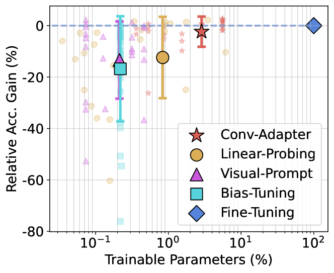
Figure 1: Performance of Conv-Adapter compared to other transfer learning methods on ResNet-50 BiT-M. We compute the relative performance gain w.r.t to fine-tuning and percentage of trainable parameters of the backbone (w/o linear head) on 23 image classification datasets from various domains to compute the results, with mean and standard deviation highlighted. Conv-Adapter achieves a superior trade-off between transfer accuracy and parameter efficiency.

Prior arts on fine-tuning ConvNets to multiple visual domains are restrictive in generalization and parameter efficiency. Bias Tuning (Ben Zaken, Goldberg, and Ravfogel 2022), which tunes only the bias terms of the backbone, might fail on domains with significant distribution shifts from the pre-training tasks. Residual Adapter (Rebuffi, Bilen, and Vedaldi 2018) and TinyTL (Cai et al. 2020) are mainly designed for small networks such as ResNet-26 (He et al. 2016) and MobileNet (Howard et al. 2017; Cai, Zhu, and Han 2019). It is prohibitive to scale these previous designs to larger ConvNets (Liu et al. 2022b) or more diverse domains (Zhai et al. 2019). Besides, previous PET methods (Houlsby et al. 2019b; Hu et al. 2021; Li and Liang 2021; Lester, Al-Rfou, and Constant 2021; He et al. 2022) are mainly designed with Transformer (Vaswani et al. 2017) architecture for NLP tasks (Devlin et al. 2018; Brown et al. 2020). However, it is not straightforward to apply Transformer-based PET to ConvNets because Transformers tokenize and sequentialize the input and features, while ConvNets do not. Recent works (Jia et al. 2022; Bahng et al. 2022; Chen et al. 2022) that attempt to use Prompt Tuning (Lester, Al-Rfou, and Constant 2021) and Adapters (Houlsby et al. 2019b) on CV tasks are also designed for Vision Transformers rather than ConvNets. Furthermore, the downstream CV tasks are usually more diverse with a larger domain gap compared with NLP (Radford et al. 2021). These challenges motivate us to design the architecture and adapting scheme of PET for ConvNets, which could make it transferable to various CV tasks, including image classification, object detection, and semantic segmentation.

In this work, we narrow the gap of PET between NLP and CV with the proposal of Conv-Adapter – an adaption module that is light-weight, domain-transferable, and architecture-agnostic. Conv-Adapter learns task-specific knowledge on downstream tasks and adapts the intermediate features of each residual block in the pre-trained ConvNets. It has a bottleneck structure consisting of depth-wise separable convolutions (Howard et al. 2017) and non-linearity. Due to the variety of CV network architectures and tasks, we explore four adapting schemes of Conv-Adapter combining two design perspectives - adapted representations and insertion form to verify the optimal tuning paradigm. We find it is essential for Conv-Adapter to maintain the locality relationship when adapting intermediate feature maps for transferability. More importantly, Conv-Adapter can be formulated under the same mathematical framework as the PET modules used in the NLP field (He et al. 2022). Conv-Adapter outperforms previous PET baselines and achieves similar or even better performance to the traditional full fine-tuning on $23$ cross-domain classification datasets with an average of $3.5$% of the backbone parameters using ResNet-50 BiT-M (Kolesnikov et al. 2019), as shown in Fig. 1. Conv-Adapter also well generalizes to object detection and semantic segmentation tasks with same-level performance to fully fine-tuning. To further understand Conv-Adapter, in addition, we empirically analyze the performance of Conv-Adapter with both the domain shifting of datasets and the network weights shifting brought by fine-tuning. The core contributions of this work can be summarized as:

• To our knowledge, we are the first to systematically investigate the feasible solutions of general parameter-efficient tuning (PET) for ConvNets. This investigation can narrow the gap between NLP and CV for PET.

• We propose Conv-Adapter, a light-weight and plug-and-play PET module, along with four adapting variants following two design dimensions - transferability and parameter efficiency. Meanwhile, we empirically justify several essential design choices to make Conv-Adapter effectively transferred to different CV tasks.

• Extensive experiments demonstrate the effectiveness and efficiency of Conv-Adapter. It achieves comparable or even better performance to full fine-tuning with only around 5% backbone parameters. Conv-Adapter also well generalizes to detection and segmentation tasks that require dense predictions.

2 Related Work

2.1 Parameter Efficient Tuning for Transformers

Pre-trained Transformer models in NLP are usually of the size of billions of parameters (Devlin et al. 2018; Brown et al. 2020; Fedus, Zoph, and Shazeer 2021), which makes fine-tuning inefficient as one needs to train and maintain a separate copy of the backbone parameters on each downstream task. Adapter (Houlsby et al. 2019b) is first proposal to conduct transfer with light-weight adapter modules. It learns the task-specific knowledge and composes it into the pre-trained backbone (Pfeiffer et al. 2020, 2021) when adapting to a new task. Similarly, LoRA introduces trainable low-rank matrices to each layer of the backbone model to approximate parameter updates. Different from inserting adaption modules to intermediate layers, Prefix Tuning (Li and Liang 2021) and Prompt Tuning (Lester, Al-Rfou, and Constant 2021), inspired by the success of textual prompts (Brown et al. 2020; Liu et al. 2021a; Radford et al. 2021), prepend learnable prompt tokens to input and only train these tokens when transferring to a new task. More recently, He et al. (2022) proposes a unified formulation of Adapter, LoRA, and Prefix Tuning, where their core function is to adapt the intermediate representation of the pre-trained model by residual task-specific representation learned by tuning modules.

Visual Prompt Tuning (Jia et al. 2022) is a recent method adapting Prompt Tuning from NLP to Vision Transformers (Jia et al. 2022). Bahng et al. (2022) also explores visual prompts in input pixel space for adapting CLIP models (Radford et al. 2021) and makes connection with (Elsayed, Goodfellow, and Sohl-Dickstein 2018). While showing promising results on Transformers, visual prompts on ConvNets presents much worse transfer results (Jia et al. 2022; Bahng et al. 2022), possibly due to the limited capacity of input space visual prompts. Conv-Adapter can adapt the intermediate features thus has larger capacity.

2.2 Transfer Learning for ConvNets

While there is no straightforward approach to applying previous PET methods designed for Transformers directly on ConvNets, several attempts have been made in prior research. BatchNorm Tuning (Mudrakarta et al. 2018) and Bias Tuning (Ben Zaken, Goldberg, and Ravfogel 2022) only tune the batchnorm related terms or the bias terms of the pre-trained backbone. Piggyback (Mallya, Davis, and Lazebnik 2018) instead learns weight masks for downstream tasks while keeping the pre-trained backbone unchanged. They all have limited transferability and update partial parameters of the backbone.

More related to our work, Residual Adapter (Rebuffi, Bilen, and Vedaldi 2018) explores inserting an extra convolutional layer of kernel size 1 to each convolutional layer in pre-trained ResNet-26 (He et al. 2016), either in parallel or in sequential, to conduct the multi-domain transfer. Similarly, TinyTL introduces extra residual blocks to MobileNet (Howard et al. 2017; Cai, Zhu, and Han 2019) for memory efficient on-device learning. Guo et al. (2019) proposes re-composing a ResNet with depth-wise and point-wise convolutions, and re-training only the depth-wise part during fine-tuning. RepNet (Yang, Rakin, and Fan 2022) exploits a dedicated designed side network to re-program the intermediate features of pre-trained ConvNets. Conv-Adapter differs from previous methods with a design that considers parameter efficiency and transferability from the internal architectures and adapting schemes. Besides, the proposed Conv-Adapter does not require tuning any backbone parameters to achieve comparable performance to fine-tuning.

3 Method

3.1 Preliminaries

Parameter efficient tuning (PET) methods (Houlsby et al. 2019b; Hu et al. 2021; Li and Liang 2021; Lester, Al-Rfou, and Constant 2021; Jia et al. 2022) introduce learnable adapting modules plugged into the backbone that is frozen during tuning. From a unified point of view, the core function of the adaption modules is to learn task-specific feature modulations on originally hidden representations in the pre-trained backbone (He et al. 2022). Specifically, considering an intermediate hidden representation $\mathbf{h}$ generated by a layer or a series of layers with input $\mathbf{x}$ in a pre-trained network, the PET adaption module learns $\Delta\mathbf{h}$ and updates $\mathbf{h}$ as:

$$\mathbf{h}\xleftarrow{}\mathbf{h}+\mathbf{\alpha}\cdot\Delta\mathbf{h},$$ (1)

where $\mathbf{\alpha}$ could be a scalar (Hu et al. 2021) or a gating function (Li and Liang 2021). Previous PET methods in NLP mainly follow a similar functional form for constructing $\Delta\mathbf{h}$ – down-sampling projection, non-linearity, and up-sampling projection. However, they differ in 1) implementation (architecture) - the form of the projections and non-linearity, and 2) the adapting scheme - which $\mathbf{h}$ in the model to adapt and compute $\Delta\mathbf{h}$ from which representation. These differences characterize the adaptation to new tasks and robustness to out-of-distribution evaluation (Li and Liang 2021).

It is non-trivial to design effective PET methods for ConvNets because previous PET modules are mainly developed on Transformers rather than ConvNets. Besides, the components of the architecture and computation dynamics of ConvNets and Transformers are inherently different. Following the unified formulation of PET methods in Eq. (1), we propose Conv-Adapter. We construct the $\Delta\mathbf{h}$ of Conv-Adapter similarly to previous PET methods and design the adaption architecture and scheme on ConvNets from the perspective of transferability and parameter efficiency.

3.2 Motivation

Before delving into the details of our design, we identify the essential difficulty that prevents utilizing prior arts directly on ConvNets as an adaption module and thus inspires us to propose Conv-Adapter. Conventionally, for ConvNets, $\mathbf{h}$ and $\Delta\mathbf{h}$ are usually 3-dimensional structural features maps belonging to $\mathbb{R}^{C\times H\times W}$ with $C$ being the channel dimension and $H\times W$ being the spatial size of the feature maps.

The difference in intermediate feature and processing dynamics poses obstacles to transferability. For Transformers, $\mathbf{h}$ is whereas 2-dimensional sequential features in $\mathbb{R}^{L\times D}$ where $L$ is the sequence length and $D$ is the feature dimension. Previous PET modules for Transformers compute $\Delta\mathbf{h}$ in various forms, e.g., linear layers over $\mathbf{h}$ (Houlsby et al. 2019b) and self-attention over additional input prompts (Li and Liang 2021; Lester, Al-Rfou, and Constant 2021; Jia et al. 2022). They can all process the sequential features globally with long-range dependencies as the computing blocks in Transformers. Although it is possible to apply linear layers, or equivalently $1\times 1$ convolutional layers (Rebuffi, Bilen, and Vedaldi 2018), to adapt the feature maps of ConvNets, it is yet intuitive that this might produce inferior transfer performance due to the loss of locality, which is encoded in the structural features maps by convolutions of kernel size larger than 1. The loss of locality results in a radical mismatch of the receptive field in $\Delta\mathbf{h}$ and $\mathbf{h}$, which might be destructive when adapting ConvNets on tasks with significant domain shifts. Apart from the receptive field mismatch, the spatial size of feature maps in ConvNets also significantly affects the transferability of adaption. Earlier attempts to use adapters to transfer ConvNets usually downsample the feature’s spatial size for memory and parameter efficiency. However, for CV tasks beyond image classification like segmentation, the spatial size matters for achieving good results (Shelhamer, Long, and Darrell 2017; Chen et al. 2017).

In summary, it is crucial to design the architecture and adapting scheme of the PET module computing $\Delta\mathbf{h}$ for ConvNets to have the same spatial size of feature maps and the same receptive field of convolutions for transferability.

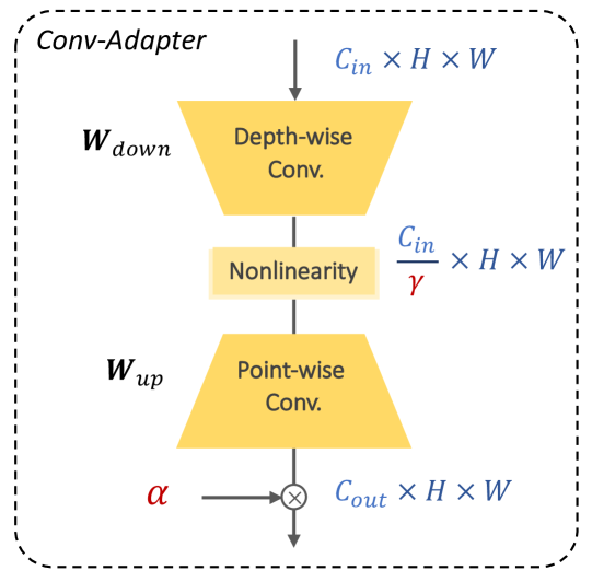
Figure 2: Architecture of Conv-Adapter, which has a bottleneck composed of depth-wise separable convolutions with non-linearity activation. $C_{in}$, $C_{out}$, $H$, $W$ is set to keep the same as in backbone. $\bm{\alpha}$ and $\gamma$ are hyper-parameters to tune.

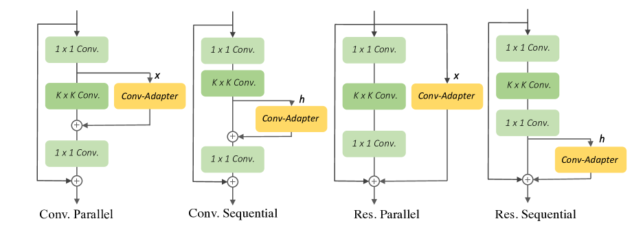
Figure 3: Four adapting schemes of Conv-Adapter to ResNet50: Convolution Parallel, Convolutional Sequential, Residual Parallel, and Residual Sequential. The schemes differ regarding the position of of the modified representation and corresponding insertion form. Other networks can be adapted similarly following the illustration. Green modules are frozen during fine-tuning.

3.3 Architecture of Conv-Adapter

Given the above challenges, we design our Conv-Adapter as a bottleneck structure, which is also widely used by PET methods of NLP tasks (He et al. 2016; Houlsby et al. 2019b). However, our Conv-Adapter designs the bottleneck, particularly for ConvNets. Precisely, it consists of two convolutional layers with a non-linearity function in-between. The first convolution conducts channel dimension down-sampling with a kernel size similar to that of the adapted blocks, whereas the second convolution projects the channel dimension back. For simplicity, we adopt the same activation function used in the backbone as the non-linearity at the middle of the bottleneck. The effective receptive field of the modulated feature maps produced by Conv-Adapter is thus similar to that of the adapted blocks in the backbone. We do not change the spatial size of the feature maps for better transferability on dense prediction tasks. We adopt the depth-wise separable convolutions (Howard et al. 2017) for Conv-Adapter to reduce the parameter size further.

Figure 2 illustrates our Conv-Adapter architecture. Formally, let the input feature map to the adapted blocks of the ConvNets be $\mathbf{z}\in\mathbb{R}^{C_{in}\times H\times W}$ and the output feature maps be $\mathbf{h}\in\mathbb{R}^{C_{out}\times H\times W}$, where $C_{in}$ and $C_{out}$ are the channel dimension of the input and output to the adapted blocks respectively. Assuming the spatial size $H\times W$ of the feature maps does not change along these blocks, we set the learnable weight as $\mathbf{W}_{down}\in\mathbb{R}^{\frac{C_{in}}{\gamma}\times\gamma\times K\times K}$ for the depth-wise convolution and $\mathbf{W}_{up}\in\mathbb{R}^{C_{out}\times\frac{C_{in}}{\gamma}\times 1\times 1}$ for the point-wise convolution in Conv-Adapter, with the non-linearity denoted as $f$. We use a compression factor of $\gamma$ to denote the down-sampling in the channel dimension, where $\gamma$ is a hyper-parameter tuned for each task. Mathematically, Conv-Adapter computes $\Delta\mathbf{h}\in\mathbb{R}^{C_{out}\times H\times W}$ as:

$$\Delta\mathbf{h}=\left(\mathbf{W}_{up}\otimes f(\mathbf{W}_{down}\hat{\otimes}\mathbf{z})\right),$$ (2)

where $\otimes$ and $\hat{\otimes}$ denotes point-wise and depth-wise convolution, respectively. To allow the modulation $\Delta\mathbf{h}$ to be more flexibly composed into $\mathbf{h}$, we set $\bm{\alpha}$ in Eq. (1) as a learnable scaling vector in $\mathbb{R}^{C_{out}}$, which is initialized as ones. The ablation study on design choices is presented in Sec. 4.5.

3.4 Adapting ConvNets with Conv-Adapter

After setting the architecture of Conv-Adapter, we discuss the scheme to adapt a variety of ConvNets. Previous PET methods insert the adapting modules to Self-Attention blocks, Feed-Forward blocks, or both (He et al. 2022) of Transformers, which have a relatively unified architecture. In contrast, modern ConvNets usually stacks either residual blocks (Szegedy et al. 2015a; He et al. 2016; Zhang et al. 2020) or inverted residual blocks (Howard et al. 2017; Tan and Le 2019, 2021; Liu et al. 2022b), which consists of a series of convolutional layers (and sometimes pooling layers) and a residual identity branch, making it more difficult to use a single adapting scheme to various architectures.

To explore the effective adapting schemes of using Conv-Adapter to tune a ConvNet, we study it mainly from two perspectives, similar to He et al. (2022), 1) the location of adaptation in pre-trained ConvNets – which intermediate representation $\mathbf{h}$ to adapt, and 2) the insertion form of Conv-Adapter – how to set the input $\mathbf{z}$ to Conv-Adapter to compute $\Delta\mathbf{h}$. From the location perspective, we study plugging Conv-Adapter to each (inverted) residual block (Cai et al. 2020) or to each functioning $K\times K$ convolutional layer within a residual block (Guo et al. 2019). From the insertion perspective, Conv-Adapter can be inserted either in parallel or in sequential to the modified components, with the input to Conv-Adapter being $\mathbf{x}$, the input to the modified components, or being $\mathbf{h}$ itself, respectively. Combining the design dimension from these two perspectives, we propose 4 variants of adapting schemes with Conv-Adapter: Convolution Parallel, Convolution Sequential, Residual Parallel, and Residual Sequential.

Taking the bottleneck residual block of ResNet-50 (He et al. 2016) as an example, we demonstrate the proposed designs in Fig. 3. As $1\times 1$ convolution layer can only transfer channel-wise information, we thus design the adapting of functional convolutions, i.e., intermediate $K\times K$ convolutions, to keep locality sensitive. On the contrary, adapting the whole residual block considers the transferring of pre-trained knowledge carried by $1\times 1$ convolutions. Intuitively, adapting the whole residual blocks has a larger capacity for modulating task-specific features than adapting only $K\times K$ convolution but may introduce more parameters. Plugging Conv-Adapter stage-wisely is not considered as it is impractical to make the receptive field of Conv-Adapter similar to the adapted stage with only two convolutions. It needs a more sophisticated design on not only the Conv-Adapter architecture but also the adaptation location (Yang, Rakin, and Fan 2022), and we empirically find that stage-wise adaptation produces inferior performance and requires much more parameters. Conv-Adapter is flexible to be inserted into every residual block of the ConvNet backbone for transferability of features from different depths, as in (Rebuffi, Bilen, and Vedaldi 2018; Mallya, Davis, and Lazebnik 2018). Other backbones such as ConvNext (Liu et al. 2022b), and even Swin-Transformer (Liu et al. 2021b) can be adapted following the same guideline (see experiments).

4 Experiments

This section verifies the transferability and parameter efficiency of Conv-Adapter from various aspects, including image classification, few-shot classification, object detection, and semantic segmentation. Additionally, we provide an ablation study of Conv-Adapter for its design choices and an analysis of its performance.

4.1 Transferability of Conv-Adapter

Setup.

We first evaluate the transferability of Conv-Adapter on classification tasks. We experiment on two benchmarks: VTAB-1k (Zhai et al. 2019) and FGVC. VTAB-1k includes 19 diverse visual classification tasks, which are grouped into three categories: Natural, Specialized, and Structured based on the domain of the images. Each task in VTAB-1k contains 1,000 training examples. FGVC consists of 4 Fine-Grained Visual Classification tasks: CUB-200-2011 (Wah et al. 2011), Stanford Dogs (Khosla et al. 2011), Stanford Cars (Krause et al. 2013), and NABirds (Van Horn et al. 2015).

For evaluation, we compare the 4 variants of Conv-Adapter with full fine-tuning (FT) and 3 baseline methods: linear probing (LP), bias tuning (Bias) (Cai et al. 2020), and visual prompt tuning (VPT) (Jia et al. 2022; Bahng et al. 2022). We test each method on ResNet50 (He et al. 2016; Kolesnikov et al. 2019) with ImageNet21k pre-training. To find the optimal hyper-parameters of Conv-Adapter (and baseline methods), we conduct a grid search of the learning rate, weight decay, and compression factor $\gamma$ for each dataset using the validation data split from training data for both benchmarks. Results are reported in Tab. 1. The details of the hyper-parameters are shown in Appendix.

Table 1: Performance of Conv-Adapter adapting schemes on ResNet-50 BiT-M. Each setting includes three runs and averaged top-1 accuracy ($\%$) over datasets and the averaged total trainable parameters (M) over all datasets are reported. We compare proposed variants of Conv-Adapter (in gray) with full Fine-Tuning (FT), Linear Probing (LP), Bias Tuning (Bias), and Visual Prompt Tuning (VPT). We report the number of wins of $(\cdot)$ for each method compared to FT. Bold and underline refer to the top and second result separately.

Tuning	# Param.	FGVC	VTAB-1k
			Natural	Specialized	Structured
# Tasks	-	4	7	4	8
FT	23.89	83.46	72.19	85.86	66.72
LP	0.37	75.44 (1)	67.42 (4)	81.42 (0)	37.92 (0)
Bias	0.41	64.98 (0)	66.06 (4)	80.34 (0)	32.18 (0)
VPT	0.42	74.79 (1)	65.43 (2)	80.35 (0)	37.64 (0)
Conv. Par.	0.85	83.77 (3)	72.60 (5)	84.21 (1)	56.70 (1)
Conv. Seq.	0.87	79.68 (2)	72.28 (4)	83.85 (0)	58.50 (1)
Res. Par.	8.21	84.24 (3)	71.75 (4)	84.70 (0)	61.34 (1)
Res. Seq.	3.53	83.45 (2)	71.74 (4)	84.84 (0)	61.33 (2)

Results and Discussion.

Conv-Adapter not only demonstrates significant improvements over the baseline methods, but also achieves the same level of performance or even surpasses their fine-tuning counterparts on all domains evaluated, by introducing only around 3.5% of full fine-tuning parameters for ResNet-50. Notably, there is a considerable performance gap, i.e., an improvement of 23.44%, of Conv-Adapter over previous baseline methods on Structured datasets of VTAB-1k.

One can observe that the proposed four variants of Conv-Adapter all achieve comparable performance compared to full fine-tuning. Among the four variants, Convolution Parallel achieves the best trade-off between performance and parameter efficiency. On the evaluated classification tasks, inserting Conv-Adapter in parallel generally outperforms inserting sequentially. In terms of the modified representation, one can find that, on most of the datasets, adapting only the $K\times K$ convolutions of ResNet-50 can achieve performance close to fine-tuning. However, on Structured datasets, adapting whole residual blocks is far better than adjusting only the middle convolutions with more parameters, demonstrating the superior capacity of adjusting residual blocks when there is a more significant domain gap.

4.2 Universality of Conv-Adapter

Setup.

We evaluate the universality of Conv-Adapter on classification tasks in this section, where Conv-Adapter is inserted to various ConvNets architectures with different pre-training. We adopt the simple yet effective adapting scheme – Convolution Parallel, and mainly compare it with full fine-tuning. More specifically, we adopt ImageNet-21k pre-trained ResNet50 (Kolesnikov et al. 2019), ConvNext-B and ConvNext-L (Liu et al. 2022b), and even Swin-B and Swin-L (Liu et al. 2021b). Apart from ImageNet-21k, we evaluate ImageNet-1K, CLIP (He et al. 2020), and MoCov3 (Chen, Xie, and He 2021) pre-training. Similarly, we conduct a hyper-parameter search on the validation set, and report the accuracy on the test set of FGVC and VTAB-1k.

Results and Discussion.

We present the results in Tab. 2. On various ImageNet-21k pre-trained ConvNets, Conv-Adapter demonstrates its universality with comparable performance to fine-tuning. For large models such as ConvNext-L and Swin-L, conducting traditional fine-tuning requires training nearly 196M parameters, whereas Conv-Adapter improves the parameter efficiency with only 7.8% and 4.5% of the fine-tuning parameters on ConvNext-L and Swin-L respectively. Although the transfer performance of Conv-Adapter on ImageNet-1k pre-trained models is more limited, compared to ImageNet-21k pre-training, Conv-Adapter still demonstrates its superior parameter efficiency and shows improvement over fine-tuning on several tasks. For the CLIP vision models, Conv-Adapter consistently outperforms fine-tuning on Structured tasks of VTAB-1k. We observe a performance gap of Conv-Adapter on MoCov3 pre-trained (Chen, Xie, and He 2021), and we argue this is possibly due to the difference in feature space of self-supervised and supervised models in CV (Jia et al. 2022).

Table 2: Comparing Conv-Adapter (CA) with full Fine-Tuning (FT) using various backbone architectures of different pre-training. Each setting includes three runs and averaged top-1 accuracy ($\%$) over datasets and the averaged total trainable parameters (M) over all datasets are reported. We report the number of wins of $(\cdot)$ for each method in compared to FT. Bold indicates the best results.

Pre-train	Backbone	Tuning	# Param.	FGVC	VTAB-1k
					Natural	Specialized	Structured
# Tasks				4	7	4	8
ImageNet 21k	ResNet50 BiT-M	FT	23.89	83.46	72.19	85.86	66.72
		CA	0.85	83.77 (3)	72.60 (5)	84.21 (1)	56.70 (1)
	ConvNext-B	FT	87.75	89.48	81.59	87.32	65.77
		CA	6.83	89.28 (1)	80.62 (4)	86.29 (0)	64.88 (2)
	ConvNext-L	FT	196.50	90.64	82.25	87.94	67.65
		CA	15.52	90.69 (3)	81.7 (2)	86.85 (0)	64.98 (3)
	Swin-B	FT	86.92	90.01	78.65	87.59	64.69
		CA	4.98	88.55 (1)	80.00 (4)	85.84 (0)	62.57 (2)
	Swin-L	FT	195.27	91.04	80.64	87.85	66
		CA	8.86	90.54 (2)	81.39 (3)	86.29 (1)	63.19 (2)
ImageNet 1k	ResNet50	FT	23.87	85.84	67.15	83.53	53.32
		CA	0.72	83.48 (0)	64.20 (0)	81.33 (1)	52.74 (2)
	ConvNext-B	FT	87.75	88.95	74.51	85.33	61.34
		CA	10.82	87.84 (1)	74.72 (4)	84.29 (0)	63.77 (2)
CLIP	ResNet50	FT	38.50	81.38	58.53	80.8	57.18
		CA	2.23	76.64 (0)	56.33 (3)	79.12 (0)	58.96 (4)
	ResNet50x4	FT	87.17	84.23	65.71	82.22	58.84
		CA	6.14	82.71 (0)	62.54 (2)	80.72 (1)	59.10 (4)
MoCov3	ResNet50	FT	23.87	83.92	66.25	83.89	60.26
		CA	0.89	79.69 (0)	65.31 (3)	81.59 (0)	53.87 (1)

4.3 Few-Shot Classification

Setup.

PET methods usually present superior performance for tasks with low-data regimes (Li and Liang 2021; He et al. 2022). We thus evaluate Conv-Adapter on few-shot classification using ImageNet-21k pre-trained ResNet50 Bit-M (Kolesnikov et al. 2019) and ConvNext-B (Liu et al. 2022b). We evaluate 5 FGVC datasets using 1, 2, 4, 8 shots for each class following following previous studies (Radford et al. 2021; Jia et al. 2022; Zhang, Zhou, and Liu 2022) including Food101 (Bossard, Guillaumin, and Van Gool 2014), Oxford Flowers (Nilsback and Zisserman 2006), Oxford Pets (Parkhi et al. 2012), Stanford Cars (Krause et al. 2013), and Aircraft (Maji et al. 2013). Averaged top-1 accuracy is reported in Tab. 3. The detailed hyper-parameters and more results for each dataset are in Appendix.

Results and Discussion.

Compared with Fine-tuning, Conv-Adapter boosts few-shot classifications with an average 3.39% margin over different shots using only around 5% trainable parameters. Especially for 1/2-shot cases, Conv-Adapter shows supreme performance compared with Fine-tuning and VPT (Jia et al. 2022) (11.07% on 1-shot and 6.99% on 2-shot with larger architecture ConvNext-B). Meanwhile, Conv-Adapter provides a better accuracy-efficiency trade-off than Visual Prompt Tuning on few-shot classifications. It surpasses VPT with an average margin of 1.35% with ResNet50 Bit-M and 3.69% with ConvNext-B. In the 8-shot case, VPT drops around 8% performance compared with Fine-tuning due to limited capacity, while Conv-Adapter can achieve comparable or better performance to Fine-tuning and maintain parameter efficiency.

Table 3: Few-shot classification: the average Top-1 accuracy over 5 FGVC datasets, with 1, 2, 4, 8 shots. We compare Conv-Adapter (CA), Visual Prompt Tuning (VPT), and full Fine-Tuning (FT). Bold indicates the best results.

Backbone	Tuning	# Param	1	2	4	8
ResNet50 Bit-M	FT	23.72	29.30	38.96	50.09	61.27
	VPT	0.24	32.56	42.18	52.21	59.37
	CA	1.02	34.31	43.55	52.43	61.42
ConvNext-B	FT	87.68	36.34	48.83	63.69	76.91
	VPT	0.13	42.25	51.85	62.89	69.04
	CA	4.6	47.41	55.82	63.25	74.29

4.4 Object Detection and Semantic Segmentation

Table 4: Object detection & Semantic Segmentation results. We report the results of fine-tuning and Conv-Adapter with the Residual Parallel scheme.

Object Detection with Faster-RCNN
Backbone	Tuning	# Param	AP	AP50	AP75
ResNet50	FT	41.53	38.1	59.7	41.5
	CA	35.72	38.4	61.1	41.5
ConvNeXt-S	FT	67.09	45.2	67.2	49.9
	CA	24.62	41.9	64.5	45.7
Semantic Segmentation with UPerNet
Backbone	Tuning	# Param (M)	mIoU
ResNet50	FT	66.49	42.1
	CA	45.65	43.0
ConvNeXt-S	FT	81.87	48.7
	CA	39.40	46.9

Setup.

Beyond image classification tasks, we also validate the generalization of Conv-Adapter on dense prediction tasks, including object detection and semantic segmentation. We use ImageNet-21k pre-trained ResNet50 and ConvNeXt-S as backbones. For object detection, we implement Conv-Adapter with Faster-RCNN using the MMDetection (Chen et al. 2019) framework compared with fine-tuning. We report the average precision (AP) results on the validation split of the MS-COCO dataset (Lin et al. 2014). For semantic segmentation, we implement Conv-Adapter with UPerNet (Xiao et al. 2018) using MMSegmentation framework (Contributors 2020) and conduct experiments on the ADE20K dataset (Zhou et al. 2017), with mIoU reported on the validation split. The detailed training setting and hyper-parameters are shown in Appendix.

Results and Discussion.

The dense prediction results are summarized in Tab. 4. We observe a different effect of Conv-Adapter on two types of backbones. On ResNet50, Conv-Adapter surpasses fine-tuning with fewer trainable parameters (including the dense prediction heads) for object detection and semantic segmentation. On ConvNeXt-S, the performance is lower than their fine-tuning counterparts. We argue that the inferior performance of Conv-Adapter on ConvNeXt-S on dense prediction tasks is due to severely reduced model capacity as the number of trainable parameters is reduced by more than 50%. Nevertheless, they can still outperform the ResNet50 with fewer total parameters. This indicates there might be overfitting issues, and we encourage more future studies on this topic.

4.5 Ablation Study

Setup.

We provide an ablation study on the design choices of Conv-Adapter, where we explore different architectures and adapting schemes. In this section, we mainly report the Top-1 accuracy on the validation set of VTAB-1k.

Architecture and Adapting Schemes.

We first compare the performance of Conv-Adapter using depth-wise separable, regular, and $1\times 1$ convolutions (linear layers). As shown in Tab. 5, depth-wise separable convolution introduces the minimal parameter budget while achieving the best results. Apart from 4 adapting variants proposed in this work, we also explore other design choices used in previous works. We experiment on spatial down-sampling of feature maps (Cai et al. 2020). Compared to channel down-sampling with a bottleneck in Conv-Adapter, spatial down-sampling introduces nearly 27 times of parameters with inferior accuracy. We also validate the adapting scheme of applying $1\times 1$ convolution to all convolutional layers (Rebuffi, Bilen, and Vedaldi 2018), which introduces nearly 16 times of parameters to Conv-Adapter with -12.27% accuracy gain. Finally, we evaluate the adapting scheme that inserts Conv-Adapter stage-wisely, which is less effective in both parameter size and performance than the proposed schemes.

Table 5: Ablation study on more adapting scheme and more architectures of Conv-Adapter. The different schemes and architectures mainly come from previous works. The proposed adaptation and architecture achieve the best results.

Adapting Scheme	Down-sample	# Convs	Type of Conv.	# Param	VTAB-1k
$K\times K$ Conv. Par.	Channel	2	Depth-wise	0.67	71.03
$K\times K$ Conv. Par.	Channel	2	Regular	5.66	70.52
$K\times K$ Conv. Par.	Channel	2	Linear	1.22	68.32
$K\times K$ Conv. Par.	Spatial	2	Depth-wise	18.45	68.54
All Conv. Par	-	1	Linear	10.74	58.75
Stage Par.	Channel	2	Depth-wise	1.90	65.06

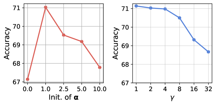
Figure 4: Sensitivity to hyper-parameters of initialization of learnable scaling vector $\bm{\alpha}$ and compression factor $\gamma$.

Sensitivity to $\gamma$ and initialization of $\bm{\alpha}$.

We explicitly study the sensitivity of the transfer performance to the initialization of the learnable scaling vector $\bm{\alpha}$ and compression factor $\gamma$ in Conv-Adapter, as shown in Fig. 4. When initializing $\bm{\alpha}$ as ones, Conv-Adapter achieves the best performance on the validation set of VTAB-1k. Compared to $\bm{\alpha}$, Conv-Adapter is more robust to the compression factor $\gamma$, achieving similar performance with the compression factor of 1, 2, and 4. Setting $\gamma$ with a larger value results in inferior performance with a more limited capacity of Conv-Adapter.

CKA Similarity and Transferability of Conv-Adapter.

We observe from Tab. 1 and Tab. 2 that, on datasets with large domain shifts, Conv-Adapter (and baseline methods) may fail to generalize well. To investigate the reason, we compute the CKA similarity (Kornblith et al. 2019; Raghu et al. 2021) between weights of convolutional filters for the pre-trained and fine-tuned backbone. The lower the CKA similarity, the larger capacity is required for good transfer performance. We plot the CKA similarity and the relative accuracy gain of Conv-Adapter to fine-tuning in Fig. 7, where the same trends over datasets exhibit for different architectures. When fully fine-tuning only leads to small changes in filter weights (larger CKA similarities), Conv-Adapter is more likely to surpass the performance of fully fine-tuning. More detail on CKA similarity comparison is in Appendix.

Figure 5: CKA similarity and accuracy gap between Conv-Adapter and fully fine-tuning for FGVC datasets.

5 Conclusions

In this work, we propose Conv-Adapter, a parameter efficient tuning module for ConvNets. Conv-Adapter is light-weight, domain-transferable, and model-agnostic. Extensive experiments on classification and dense prediction tasks show it can achieve performance comparable to full fine-tuning with much fewer parameters. We find Conv-Adapter might fail on tasks with large domain shifts and subject to feature quality determined by pre-training. Future work includes more exploration of Conv-Adapter on domain robustness and dense predictions and NAS for Conv-Adapter.

Appendix A Implementation Details

In this section, we provide more implementation details of Conv-Adapter. We first show the details of the datasets we used and the pre-trained models we used. Then we present the details of hyper-parameter used for each method and each dataset in experiments. We implement all ConvNets and Conv-Adapter in PyTorch, and the code will be made available.

A.1 Datasets

The specifications of the all datasets evaluated in experiments are shown in Tab. 6.

Table 6: Specification of all datasets evaluated. We use * to indicated randomly sampled train and validation sets (from original training set) for datasets which do not have validation split.

Dataset	Description	# Class	# Train	# Val	# Test
CUB-200-2011	FGVC	200	5,394*/5,994	600*	5,794
NABirds		700	21,536*/23,929	2,393*	24,633
Stanford Dogs		120	10,800*/12,000	1,200*	8,580
Stanford Cars		196	7,329*/8,144	815*	8,041
CIFAR-100	Natural	100	800/200	200	10,000
Caltech101		102			6,084
DTD		47			1,880
Oxford Flowers102		102			6,149
Oxford Pets		37			3,669
SVHN		10			26,032
Sun397		397			21,750
Patch Camelyon	Specialized	2	800/200	200	32,768
EuroSAT		10			5,400
Resisc45		45			6,300
Retinopathy		5			42,670
Clevr/count	Structured	8	800/200	200	15,000
Clevr/dist		6			15,000
DMLab		6			22,735
KITTI/dist		4			711
dSprites/loc		16			73,728
dSprite/ori		16			73,728
SmallNORB/azi		18			12,150
SmallNORB/ele		9			12,150
FGVCAirCraft	Few-Shot	102	shots $\times$ classes	3,333	3,333
Food101		101		20,200	30,300
Oxford Flowers102		102		1,633	2,463
Oxford Pets		37		736	3,669
Stanford Cars		196		1,635	8,041
MS-COCO	Detection	80	117,266	5,000	-
ADE-20k	Segmentation	150	25,574	2,000	-

A.2 Models

We present the details of the pre-trained models used in experiments in Tab. 7, with the checkpoint link.

Table 7: Specification of pre-trained models used in experiments.

Backbone	Pre-trained Objective	Pre-trained Dataset	# Param (M)	Feature Dim	Model
ResNet50 (He et al. 2016)	Supervised	ImageNet-1k	23.5	2,048	checkpoint
ResNet50 (He et al. 2016)	Supervised	ImageNet-21k	23.5	2,048	checkpoint
ResNet50 BiT-M (Kolesnikov et al. 2019)	Supervised	ImageNet-21k	23.5	2,048	checkpoint
ConvNext-B (Liu et al. 2022b)	Supervised	ImageNet-1k	87.6	1,024	checkpoint
ConvNext-B (Liu et al. 2022b)	Supervised	ImageNet-21k	87.6	1,024	checkpoint
ConvNext-L (Liu et al. 2022b)	Supervised	ImageNet-21k	196.2	1,536	checkpoint
Swin-B (Liu et al. 2021b)	Supervised	ImageNet-21k	86.7	1,024	checkpoint
Swin-L (Liu et al. 2021b)	Supervised	ImageNet-21k	194.9	1,536	checkpoint
ResNet50 (Radford et al. 2021)	CLIP	CLIP	38.3	1,024	checkpoint
ResNet50x4 (Radford et al. 2021)	CLIP	CLIP	87.1	640	checkpoint
ResNet50 (He et al. 2020)	MoCov3	ImageNet-1k	23.5	2,048	checkpoint

A.3 Hyper-parameters in Experiments

We provide the hyper-parameters search range and important settings used in experiments in this section. The detailed hyper-parameters used in experiments will be made available as configuration files in code.

Classification on FGVC and VTAB-1k

For classification tasks of FGVC and VTAB-1k, we summarize the hyper-parameter range in Tab. 8. For VTAB-1k, we use the recommended optimal data augmentations in (Zhai et al. 2019), rather than solely Resize and Centre Crop as in (vpt; Zhang, Zhou, and Liu 2022). We find the recommended augmentations produces better results for full-tuning. For FGVC, we use RandomResized Crop with a minimum scale of 0.2 and Horizontal Flip (Szegedy et al. 2015b) as augmentation. For few-shot classifications, we use the same range as in Tab. 8 and same augmentations as for FGVC tasks.

Table 8: Hyper-parameter range for grid-search on image classification tasks of FGVC and VTAB-1k.

	All Backbones
Optimizer	AdamW (Loshchilov and Hutter 2017)
LR Range	[1e-3, 5e-4, 1e-4, 5e-5, 1e-5]
WD Range	[1e-2, 1e-3, 1e-4, 0]
LR schedule	cosine
Total Epochs	100
Warmup	10

A.4 Dense Prediction Tasks

Object Detection

We compare all four schemes of Conv-Adapter with the fine-tuning baseline. Specifically, we follow a standard 1x training schedule: all models are trained with a batch size of 16 and optimized by AdamW with an initial learning rate of 0.0002 for Faster RCNN and 0.0001 for RetinaNet, which are then dropped by a factor of 10 at the 8-th and 11-th epoch. The shorter side of the input image is resized to 800 while maintaining the original aspect ratio.

Semantic Segmentation

We conduct similar experiments for the segmentation task. For ResNet50 backbones, we train all models for 80k iterations with an random cropping augmentation of 512 $\times$ 512 input resolution. For ConvNeXt models, we use a larger input resolution of 640 $\times$ 640 and train the models for 160k iterations. We apply AdamW optimizer with a polynomial learning rate decay schedule.

Appendix B Extended Analysis

B.1 Model Analysis

In this section, we provide an analysis of the trainable parameters, model latency, and GFLOPs, based on ResNet50 (He et al. 2016) and ConvNext-B (Liu et al. 2022b). Since Conv-Adapter is applied on each residual block, we first provide a theoretical analysis of the trainable parameters of each adapting scheme proposed in Tab. 9. Take the bottleneck residual block of ResNet50 as an example, we set the channel size for each convolution in the residual block as $C_{in}$, $C_{mid}$, and $C_{out}$ respectively, where $C_{in}$ is usually set to $\frac{C_{in}}{4}$. We assume the spatial size of the feature maps do not change at each residual block.

We also provide the measurement of training/testing latency, memory cost, and GFLOPs for all the tasks evaluated in this paper, as shown in Tab. 10. For image classification, we average the inference speed over a batch of 64. Although Conv-Adapter has increased testing latency because of the inference includes forwarding on both backbone and Conv-Adapter, the latency and memory cost of training is not necessarily greater thanks to reduced overhead of gradient computation.

Table 9: Analysis of trainable parameters of the 4 proposed adapting schemes, compared to fine-tuning.

Tuning	Input	Output	Trainable Param.
FT	$C_{in}\times H\times W$	$C_{out}\times H\times W$	$K\times K\times C_{in}\times C_{mid}+C_{in}\times C_{mid}+C_{out}\times C_{mid}$
Conv. Par	$C_{mid}\times H\times W$	$C_{mid}\times H\times W$	$K\times K\times C_{mid}+\frac{C_{mid}}{\gamma}\times C_{mid}$
Conv. Seq.	$C_{mid}\times H\times W$	$C_{mid}\times H\times W$	$K\times K\times C_{mid}+\frac{C_{mid}}{\gamma}\times C_{mid}$
Res. Par.	$C_{in}\times H\times W$	$C_{out}\times H\times W$	$K\times K\times C_{in}+\frac{C_{in}}{\gamma}\times C_{in}$
Res. Seq.	$C_{in}\times H\times W$	$C_{out}\times H\times W$	$K\times K\times C_{in}+\frac{C_{in}}{\gamma}\times C_{in}$

Table 10: Evaluation of model latency, memory, and GFLOPs of 4 proposed variants for ResNet-50 and ConvNext-B on image classification, object detection, and semantic segmentation

Image Classification, Input Res. (224 $\times$ 224)
Backbone	Tuning	Train		Test		GFLOPs
		Latency	Memory	Latency	Memory
		(ms/img)	(GB)	(ms/img)	(GB)
ResNet50-BiT	FT	1.40	7.46	0.43	2.81	4.12
	Conv. Par.	1.21	7.35	0.48	2.81	4.34
	Conv. Seq.	1.24	7.62	0.54	2.81	4.34
	Res. Par.	1.81	8.45	0.69	2.85	7.0
	Res. Seq.	1.83	9.78	0.72	2.83	7.47
ConvNeXt-B	FT	4.18	16.96	1.17	2.92	15.36
	Conv. Par.	4.91	13.52	1.70	2.98	17.53
	Conv. Seq.	4.94	14.55	1.70	2.98	17.53
	Res. Par.	4.84	13.50	1.75	2.98	17.53
	Res. Seq.	4.84	14.76	1.72	2.99	17.6
Object Detection (Test only)
Backbone	Tuning	Input Res.		Latency (ms/img)		GFLOPs
ResNet50	FT	1280 $\times$ 800		9.38		84.08
	Conv. Par.			9.37		88.61
	Conv. Seq.			11.00		88.61
	Res. Par.			17.09		142.89
	Res. Seq.			16.30		152.54
ConvNeXt-B	FT	1280 $\times$ 800		28.55		313.45
	Conv. Par.			41.00		357.66
	Conv. Seq.			41.03		357.66
	Res. Par.			41.13		357.66
	Res. Seq.			41.22		359.22
Semantic Segmentation (Test only)
ResNet50	FT	2048 $\times$ 1024		17.18		172.19
	Conv. Par.			17.21		181.47
	Conv. Seq.			20.23		181.47
	Res. Par.			29.79		292.63
	Res. Seq.			21.22		312.4
ConvNeXt-B	FT	2048 $\times$ 1024		58.67		641.95
	Conv. Par.			83.69		732.48
	Conv. Seq.			83.77		732.48
	Res. Par.			83.07		732.48
	Res. Seq.			84.21		735.69

B.2 More Ablation of Conv-Adapter

Kernel size in Conv-Adapter

We show the performance of Conv-Adapter on VTAB-1k validation set in Fig 6, of using different kernel size for the depth-wise convolution to verify our argument of the loss of locality. One can observe that, for both ResNet50 and ConvNext-B, using smaller kernel size results in inferior performance. When setting the kernel size larger to that of the residual blocks, i.e., 5 and 7 for ResNet50, the performance is further boosted, with more parameters introduced.

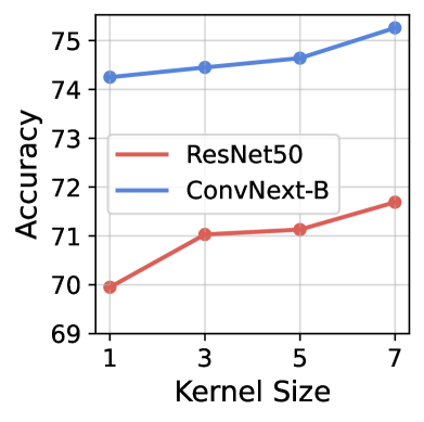
Figure 6: Sensitivity to kernel size of depth-wise convolution in Conv-Adapter, for both ResNet50 and ConvNext-B.

B.3 CKA Similarity Analysis

While the accuracy performance is well compared for PET methods, theoretical understandings towards under which circumstances PET works better than Fine-tuning lack discovery yet. In this section, we study how weights of backbones change with Fine-tuning using Centered Kernel Analysis and empirically discover insightful observations.

Similarity Measurement between Filter Weights using CKA

As shown in the experimental results, whether the performance of PET surpasses Fine-tuning varies from datasets and domains. From the perspective of trainable weights, PET replaces the whole backbone with much smaller number of parameters compared with Fine-tuning. With the pre-trained backbone and the fine-tuned backbone, we first compute the similarity between the weights of each convolution filter using Centered Kernel Alignment (CKA). In doing so, the changes of weights brought by Fine-tuning are quantified by similarity distances between filters.

CKA is used to compute the representation similarity between hidden layers of neural networks (Kornblith et al. 2019; Raghu et al. 2021). By inputting matrices $\mathbf{X}\in\mathbb{R}^{n\times m_{1}}$, $\mathbf{Y}\in\mathbb{R}^{n\times m_{2}}$, and their Gram matrices $\mathbf{K}=\mathbf{X}\mathbf{X}^{T}$ and $\mathbf{L}=\mathbf{Y}\mathbf{Y}^{T}$, CKA follows:

$$\operatorname{CKA}(\mathbf{K},\mathbf{L})=\frac{\operatorname{HSIC}(K,L)}{\sqrt{\operatorname{HSIC}(K,K)\operatorname{HSIC}(L,L)}}$$

Where $\operatorname{HSIC}$ is the Hilbert-Schmidt independence criterion. Instead of analyzing the representation similarity, we focus on analyzing how filter weights change by Fine-tuning and utilize CKA to compute the similarity between filter weights. For each $k\times k$ convolution layer with $c_{1}$ input channels and $c_{2}$ output channels, weights from the initial pre-trained backbone is referred as $\mathbf{W}_{i}$ and weights from the fine-tuned backbone is referred as $\mathbf{W}_{f}$. The filter weights are reshaped into matrices for CKA computation:

• For $k=1$, the convolutional filter serves as a linear transformation between channels. When computing CKA similarity, $X=\mathbf{W}_{i},\mathbf{W}_{i}\in\mathbb{R}^{c_{1}\times c_{2}}$ and $Y=\mathbf{W}_{f},\mathbf{W}_{f}\in\mathbb{R}^{c_{1}\times c_{2}}$.

• for $k>1$, the weight matrix can be viewed as $c_{1}\times c_{2}$ filters and each filter carries a size of $k\times k$ weights. When computing CKA similarity, $X=\mathbf{W}_{i},\mathbf{W}_{i}\in\mathbb{R}^{k^{2}\times c_{1}c_{2}}$, $Y=\mathbf{W}_{f},\mathbf{W}_{f}\in\mathbb{R}^{k^{2}\times c_{1}c_{2}}$.

For each ConvNet, we compute the average of CKA similarities among all convolutional filters and show the results of ResNet, ConvNext and ResNet-CLIP in Fig. 7. With a relatively low accuracy of Finetuning, the similarity between filter weights may not be well representative due to insufficient optimization. Thus NABirds is removed in the analysis. We also measure the domain difference between datasets with ImageNet1k using Maximum Mean Discrepancy ( Details are in the following section). Firstly we observe that with less domain difference between target dataset and pre-trained dataset, the Conv-Adapter achieves closer performance with fully finetuning. Secondly, as shown in Fig. 7, accuracy gain of Conv-Adapter and CKA similarities between filter weights share the same trends over datasets and this phenomenon generalizes over different architectures. When fully finetuning only leads to small changes on filter weights (larger CKA similarities), Conv-Adapter is more likely to surpass the performance of fully finetuning.

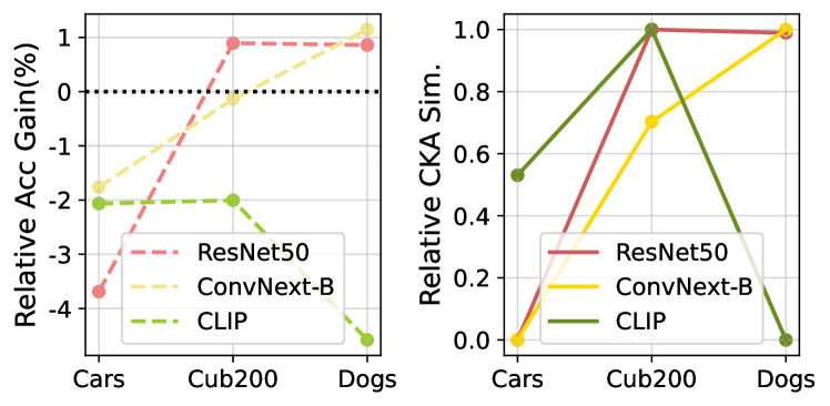
Figure 7: CKA Similarity and Accuracy gap between Conv-Adapter and fully fine-tuning for FGVC datasets.

Domain Difference Quantification using MMD (Maximum Mean Discrepancy)

Maximum Mean Discrepancy (MMD): measures the distance between two data distributions $p$ and $q$. $\phi()$ refers to a feature extractor (could be a functional intermediate layer):

$$\operatorname{MMD}(p,q)=\|\mathbf{E}_{p}[\phi(\mathbf{x})]-\mathbf{E}_{q}[\phi(\mathbf{x}]\|_{\mathcal{H}_{k}}^{2}$$ (3)

$\mathcal{H}_{k}$ refers to the kernel Hilbert space. We consider the domain difference between ImageNet1k and each dataset from FGVC. Specifically, The features subtracted from pre-trained backbones namely ResNet50 (pre-trained by Imagenet1K, ImageNet21K and CLIP), ConvNext-B (pretrained by ImageNet1K and ImageNet21K). MMD with Gaussian Kernel is computed using features from each backbone and the average MMD over all backbones is used in Fig. 7.

Appendix C Supplementary Results

In this section, we provide some supplementary results to the main paper.

C.1 Detailed Results on FGVC

We provide the per-task results on FGVC on ResNet50 BiT-M (Kolesnikov et al. 2019) and ConvNext-B (Liu et al. 2022b) in Tab. 11 and Tab. 12 respectively.

Table 11: Per-task FGVC results of ImageNet-21k pre-trained ResNet50 BiT-M.

Tuning	# Param	CUB200	Stanford Dogs	Stanford Cars	NABirds
FT	24.15	84.51±0.08	79.75±0.08	89.59±0.25	79.97±0.15
LP	0.63	86.07±0.13	80.48±0.07	64.31±0.26	70.89±0.02
Bias	0.67	79.13±0.28	76.49±0.11	34.63±0.1	69.68±0.11
VPT	0.69	85.96±0.1	79.58±0.11	56.9±0.46	76.72±0.1
Conv. Par.	1.22	86.41±0.2	82.07±0.1	85.78±0.25	80.83±0.09
Conv. Seq.	1.06	85.48±0.19	80.5±0.09	73.47±11.62	79.27±0.15
Res. Par.	7.82	85.98±0.15	81.91±0.11	88.96±0.05	80.13±0.16
Res. Seq.	11.80	85.85±0.22	80.69±0.01	87.59±0.16	79.68±0.12

Table 12: Per-task FGVC results of ImageNet-21k pre-trained ConvNext-B.

Tuning	# Param	CUB200	Stanford Dogs	Stanford Cars	NABirds
FT	87.87	89.31±0.18	87.18±0.07	93.43±0.24	88.01±0.17
LP	0.31	90.46±0.02	89.86±0.1	74.96±0.06	85.76±0.02
Bias	0.44	90.86±0.07	89.46±0.03	92.05±0.12	88.25±0.04
VPT	0.37	89.83±0.02	89.95±0.12	74.64±0.06	85.69±0.05
Conv. Par.	5.81	89.83±0.22	88.38±0.34	91.83±0.18	87.06±0.07
Conv. Seq.	3.11	76.5±18.24	86.77±0.28	91.32±0.23	87.4±0.05
Res. Par.	5.73	90.09±0.08	88.06±0.18	90.78±0.14	86.53±0.06
Res. Seq.	8.04	88.57±0.07	87.68±0.07	91.61±0.1	87.03±0.04

C.2 Detailed Results on VTAB-1k

We provide the per-task results on VTAB-1k on ResNet50 BiT-M (Kolesnikov et al. 2019) and ConvNext-B (Liu et al. 2022b) in Tab. 13 and Tab. 14 respectively.

Table 13: Per-task VTAB-1k results of ImageNet-21k pretrained ResNet50 BiT-M.

Tuning	# Param	Caltech101	Cifar100	DTD	Flowers102	Pets	Sun397	SVHN	Patch Camelyon	EuroSAT	Resisc45	Diabetic Retinopathy	Clevr/count	Clevr/dist	Dmlab	Dsprites/loc	Dsprites/ori	Kitti	Smallnorb/azi	Smallnorb/ele
FT	23.63	84.79±0.46	48.28±0.56	65.32±0.3	97.5±0.05	86.74±0.46	38.14±0.24	84.57±0.91	85.2±0.39	95.46±0.17	84.03±0.15	78.74±0.11	96.77±1.37	58.15±0.3	51.17±0.08	94.39±0.96	69.77±0.68	78.99±0.46	41.79±0.62	42.74±0.19
LP	0.11	84.35±0.51	44.02±0.18	66.49±0.15	98.85±0.03	88.16±0.23	43.24±0.58	46.8±0.06	79.88±0.33	92.53±0.15	78.65±0.24	74.64±0.08	50.43±0.09	33.91±0.19	37.92±0.16	34.23±0.07	33.67±0.09	66.95±0.34	18.27±0.19	27.96±0.09
Bias	0.15	83.75±0.08	41.99±0.4	66.31±0.35	97.84±0.04	87.91±0.45	39.29±0.21	45.34±0.3	79.82±0.19	91.07±0.03	75.77±0.62	74.72±0.04	41.97±0.13	33.27±0.17	37.86±0.03	18.4±0.13	19.43±0.43	67.32±0.26	13.59±0.23	25.55±0.44
VPT	0.15	83.4±0.87	34.92±0.15	59.06±0.13	98.1±0.38	86.14±0.37	43.34±0.22	53.08±0.31	81.06±0.99	91.04±0.09	75.07±0.21	74.25±0.09	49.2±0.43	46.25±0.31	38.64±0.16	41.87±0.93	33.53±2.25	43.84±31.0	20.6±0.53	27.2±0.49
Conv. Par.	0.48	85.26±0.49	48.29±0.07	68.79±0.44	98.28±0.18	86.16±0.03	43.9±0.34	77.55±0.18	84.25±0.59	95.45±0.13	80.67±0.17	76.48±0.21	78.57±1.45	49.17±0.42	46.37±0.73	68.3±6.06	70.55±0.75	78.11±0.52	27.84±0.71	34.69±0.22
Conv. Seq.	0.67	83.43±0.49	48.92±0.38	68.09±0.64	97.89±0.25	85.75±0.35	42.78±0.17	79.11±1.13	84.08±0.55	94.23±0.17	80.78±0.53	76.32±0.09	73.73±2.04	50.61±0.47	46.16±0.2	85.51±3.07	71.7±0.63	75.76±1.57	30.52±0.24	34.03±0.22
Res. Par.	4.61	85.94±0.57	44.2±0.77	67.29±0.67	98.1±0.02	86.57±0.6	40.4±1.93	79.75±0.61	84.07±0.62	94.84±0.31	83.3±0.13	76.59±0.09	84.18±1.87	54.83±1.03	45.42±0.61	95.78±0.23	66.81±0.58	76.98±0.59	30.72±0.62	35.97±0.43
Res. Seq.	7.06	85.4±0.49	45.27±0.76	65.44±0.37	98.18±0.05	86.21±0.17	42.18±0.1	79.53±0.32	84.9±0.37	95.38±0.12	82.43±0.52	76.67±0.15	79.23±1.13	56.54±1.45	48.02±0.58	96.38±0.62	70.41±0.23	72.85±1.21	31.17±1.0	36.05±0.08

Table 14: Per-task VTAB-1k results of ImageNet-21k pre-trained ConvNext-B.

Tuning	# Param	Caltech101	Cifar100	DTD	Flowers102	Pets	Sun397	SVHN	Patch Camelyon	EuroSAT	Resisc45	Diabetic Retinopathy	Clevr/count	Clevr/dist	Dmlab	Dsprites/loc	Dsprites/ori	Kitti	Smallnorb/azi	Smallnorb/ele
FT	87.62	91.97±0.69	69.06±0.42	76.15±0.28	99.55±0.02	92.12±0.26	52.48±0.19	89.78±0.22	86.41±0.31	96.08±0.16	88.32±0.26	78.48±0.27	93.78±0.98	55.9±5.55	56.06±0.67	96.35±0.18	70.21±0.81	78.44±0.74	39.15±0.47	36.29±0.39
LP	0.05	89.48±0.11	60.53±0.28	75.71±0.07	99.58±0.01	92.02±0.15	57.44±0.17	55.96±0.15	83.13±0.36	93.59±0.18	82.78±0.3	75.74±0.0	55.39±0.1	37.69±0.04	43.1±0.07	26.01±0.06	37.72±0.03	67.23±0.71	19.94±0.1	27.71±0.17
Bias	0.18	89.14±0.75	61.38±0.31	76.33±0.04	99.65±0.02	90.64±0.97	51.26±0.31	86.38±0.19	85.76±0.32	95.33±0.18	83.71±0.18	77.17±0.35	74.3±1.65	48.27±0.47	52.19±0.48	93.78±1.71	65.5±0.83	75.34±1.26	31.51±0.34	29.18±0.23
VPT	0.10	89.79±0.46	57.8±0.23	73.46±0.22	99.58±0.03	92.3±0.22	55.55±0.1	58.33±0.24	83.11±0.16	93.13±0.2	83.01±0.12	74.76±0.38	58.58±0.45	46.52±0.76	39.0±0.47	53.09±0.52	27.38±3.56	64.93±0.43	20.75±0.46	31.44±1.06
Conv. Par.	7.83	90.94±0.32	66.0±0.06	74.91±0.44	98.81±0.21	92.4±0.18	52.87±0.26	88.44±0.46	85.96±0.17	95.61±0.08	85.72±0.25	77.86±0.11	86.53±1.66	59.48±1.19	55.0±0.19	93.67±0.65	67.11±0.78	83.5±0.88	39.01±0.21	34.72±0.21
Conv. Seq.	9.58	90.28±0.31	68.28±0.94	76.22±0.54	98.48±0.09	91.29±0.08	53.43±0.27	88.03±0.25	86.32±0.05	94.98±0.24	85.64±0.18	77.69±0.16	91.17±0.7	51.15±6.0	52.88±0.44	90.58±0.79	68.22±0.24	83.08±0.83	38.26±0.66	37.41±0.79
Res. Par.	9.14	91.41±0.9	64.98±0.25	73.33±0.5	99.43±0.02	91.66±0.28	52.21±0.21	88.94±0.38	85.59±0.34	95.51±0.13	84.51±0.22	77.58±0.21	89.23±0.41	56.34±0.99	55.14±0.13	90.88±0.1	65.65±0.52	81.25±1.19	38.1±0.28	37.78±0.4
Res. Seq.	10.73	89.26±1.24	63.75±0.76	74.61±0.33	99.33±0.11	90.69±0.34	51.37±0.38	88.47±0.45	85.77±0.27	95.57±0.13	85.47±0.7	77.72±0.12	91.54±0.47	52.26±1.89	55.06±0.51	61.9±1.12	64.35±0.49	82.93±0.07	36.74±0.2	38.72±1.47

References

- Bahng et al. (2022) Bahng, H.; Jahanian, A.; Sankaranarayanan, S.; and Isola, P. 2022. Exploring Visual Prompts for Adapting Large-Scale Models. arXiv preprint arXiv:2203.17274.
- Ben Zaken, Goldberg, and Ravfogel (2022) Ben Zaken, E.; Goldberg, Y.; and Ravfogel, S. 2022. BitFit: Simple Parameter-efficient Fine-tuning for Transformer-based Masked Language-models. Proceedings of the 60th Annual Meeting of the Association for Computational Linguistics (Volume 2: Short Papers).
- Bommasani et al. (2021) Bommasani, R.; Hudson, D. A.; Adeli, E.; Altman, R.; Arora, S.; et al. 2021. On the Opportunities and Risks of Foundation Models. arXiv:2108.07258.
- Bossard, Guillaumin, and Van Gool (2014) Bossard, L.; Guillaumin, M.; and Van Gool, L. 2014. Food-101 – Mining Discriminative Components with Random Forests. In European Conference on Computer Vision.
- Brown et al. (2020) Brown, T. B.; Mann, B.; Ryder, N.; Subbiah, M.; Kaplan, J.; Dhariwal, P.; Neelakantan, A.; Shyam, P.; Sastry, G.; Askell, A.; Agarwal, S.; Herbert-Voss, A.; Krueger, G.; Henighan, T.; Child, R.; Ramesh, A.; Ziegler, D. M.; Wu, J.; Winter, C.; Hesse, C.; Chen, M.; Sigler, E.; Litwin, M.; Gray, S.; Chess, B.; Clark, J.; Berner, C.; McCandlish, S.; Radford, A.; Sutskever, I.; and Amodei, D. 2020. Language Models are Few-Shot Learners. arXiv:2005.14165.
- Cai et al. (2020) Cai, H.; Gan, C.; Zhu, L.; and Han, S. 2020. TinyTL: Reduce Memory, Not Parameters for Efficient On-Device Learning. In Larochelle, H.; Ranzato, M.; Hadsell, R.; Balcan, M.; and Lin, H., eds., Advances in Neural Information Processing Systems, volume 33, 11285–11297. Curran Associates, Inc.
- Cai, Zhu, and Han (2019) Cai, H.; Zhu, L.; and Han, S. 2019. ProxylessNAS: Direct Neural Architecture Search on Target Task and Hardware. In International Conference on Learning Representations.
- Chen et al. (2019) Chen, K.; Wang, J.; Pang, J.; Cao, Y.; Xiong, Y.; Li, X.; Sun, S.; Feng, W.; Liu, Z.; Xu, J.; Zhang, Z.; Cheng, D.; Zhu, C.; Cheng, T.; Zhao, Q.; Li, B.; Lu, X.; Zhu, R.; Wu, Y.; Dai, J.; Wang, J.; Shi, J.; Ouyang, W.; Loy, C. C.; and Lin, D. 2019. MMDetection: Open MMLab Detection Toolbox and Benchmark. arXiv preprint arXiv:1906.07155.
- Chen et al. (2017) Chen, L.-C.; Papandreou, G.; Schroff, F.; and Adam, H. 2017. Rethinking atrous convolution for semantic image segmentation. arXiv preprint arXiv:1706.05587.
- Chen et al. (2022) Chen, S.; Ge, C.; Tong, Z.; Wang, J.; Song, Y.; Wang, J.; and Luo, P. 2022. AdaptFormer: Adapting Vision Transformers for Scalable Visual Recognition. arXiv:2205.13535.
- Chen, Xie, and He (2021) Chen, X.; Xie, S.; and He, K. 2021. An Empirical Study of Training Self-Supervised Vision Transformers. arXiv preprint arXiv:2104.02057.
- Contributors (2020) Contributors, M. 2020. MMSegmentation: OpenMMLab Semantic Segmentation Toolbox and Benchmark. https://github.com/open-mmlab/mmsegmentation.
- Devlin et al. (2018) Devlin, J.; Chang, M.-W.; Lee, K.; and Toutanova, K. 2018. BERT: Pre-training of Deep Bidirectional Transformers for Language Understanding. arXiv:1810.04805.
- Dosovitskiy et al. (2020) Dosovitskiy, A.; Beyer, L.; Kolesnikov, A.; Weissenborn, D.; Zhai, X.; Unterthiner, T.; Dehghani, M.; Minderer, M.; Heigold, G.; Gelly, S.; Uszkoreit, J.; and Houlsby, N. 2020. An Image is Worth 16x16 Words: Transformers for Image Recognition at Scale. arXiv:2010.11929.
- Elsayed, Goodfellow, and Sohl-Dickstein (2018) Elsayed, G. F.; Goodfellow, I.; and Sohl-Dickstein, J. 2018. Adversarial Reprogramming of Neural Networks. arXiv:1806.11146.
- Fedus, Zoph, and Shazeer (2021) Fedus, W.; Zoph, B.; and Shazeer, N. 2021. Switch Transformers: Scaling to Trillion Parameter Models with Simple and Efficient Sparsity. arXiv:2101.03961.
- Guo et al. (2019) Guo, Y.; Li, Y.; Wang, L.; and Rosing, T. 2019. Depthwise Convolution Is All You Need for Learning Multiple Visual Domains. Proceedings of the AAAI Conference on Artificial Intelligence, 33: 8368–8375.
- He et al. (2022) He, J.; Zhou, C.; Ma, X.; Berg-Kirkpatrick, T.; and Neubig, G. 2022. Towards a Unified View of Parameter-Efficient Transfer Learning. In International Conference on Learning Representations.
- He et al. (2020) He, K.; Fan, H.; Wu, Y.; Xie, S.; and Girshick, R. 2020. Momentum Contrast for Unsupervised Visual Representation Learning. 2020 IEEE/CVF Conference on Computer Vision and Pattern Recognition (CVPR).
- He et al. (2016) He, K.; Zhang, X.; Ren, S.; and Sun, J. 2016. Deep Residual Learning for Image Recognition. 2016 IEEE Conference on Computer Vision and Pattern Recognition (CVPR).
- Houlsby et al. (2019a) Houlsby, N.; Giurgiu, A.; Jastrzebski, S.; Morrone, B.; De Laroussilhe, Q.; Gesmundo, A.; Attariyan, M.; and Gelly, S. 2019a. Parameter-Efficient Transfer Learning for NLP. In Chaudhuri, K.; and Salakhutdinov, R., eds., Proceedings of the 36th International Conference on Machine Learning, volume 97 of Proceedings of Machine Learning Research, 2790–2799. PMLR.
- Houlsby et al. (2019b) Houlsby, N.; Giurgiu, A.; Jastrzebski, S.; Morrone, B.; De Laroussilhe, Q.; Gesmundo, A.; Attariyan, M.; and Gelly, S. 2019b. Parameter-Efficient Transfer Learning for NLP. In Proceedings of the 36th International Conference on Machine Learning.
- Howard et al. (2017) Howard, A. G.; Zhu, M.; Chen, B.; Kalenichenko, D.; Wang, W.; Weyand, T.; Andreetto, M.; and Adam, H. 2017. MobileNets: Efficient Convolutional Neural Networks for Mobile Vision Applications. arXiv:1704.04861.
- Hu et al. (2021) Hu, E.; Shen, Y.; Wallis, P.; Allen-Zhu, Z.; Li, Y.; Wang, L.; and Chen, W. 2021. LoRA: Low-Rank Adaptation of Large Language Models. arXiv:2106.09685.
- Jia et al. (2022) Jia, M.; Tang, L.; Chen, B.-C.; Cardie, C.; Belongie, S.; Hariharan, B.; and Lim, S.-N. 2022. Visual Prompt Tuning. In European Conference on Computer Vision (ECCV).
- Khosla et al. (2011) Khosla, A.; Jayadevaprakash, N.; Yao, B.; and Fei-Fei, L. 2011. Novel Dataset for Fine-Grained Image Categorization. In First Workshop on Fine-Grained Visual Categorization, IEEE Conference on Computer Vision and Pattern Recognition. Colorado Springs, CO.
- Kolesnikov et al. (2019) Kolesnikov, A.; Beyer, L.; Zhai, X.; Puigcerver, J.; Yung, J.; Gelly, S.; and Houlsby, N. 2019. Big Transfer (BiT): General Visual Representation Learning. arXiv:1912.11370.
- Kornblith et al. (2019) Kornblith, S.; Norouzi, M.; Lee, H.; and Hinton, G. 2019. Similarity of neural network representations revisited. In International Conference on Machine Learning, 3519–3529. PMLR.
- Krause et al. (2013) Krause, J.; Stark, M.; Deng, J.; and Fei-Fei, L. 2013. 3D Object Representations for Fine-Grained Categorization. In 4th International IEEE Workshop on 3D Representation and Recognition (3dRR-13). Sydney, Australia.
- Lester, Al-Rfou, and Constant (2021) Lester, B.; Al-Rfou, R.; and Constant, N. 2021. The Power of Scale for Parameter-Efficient Prompt Tuning. In Proceedings of the 2021 Conference on Empirical Methods in Natural Language Processing, 3045–3059. Online and Punta Cana, Dominican Republic: Association for Computational Linguistics.
- Li and Liang (2021) Li, X. L.; and Liang, P. 2021. Prefix-Tuning: Optimizing Continuous Prompts for Generation. arXiv:2101.00190.
- Lin et al. (2014) Lin, T.-Y.; Maire, M.; Belongie, S.; Bourdev, L.; Girshick, R.; Hays, J.; Perona, P.; Ramanan, D.; Zitnick, C. L.; and Dollár, P. 2014. Microsoft COCO: Common Objects in Context. Cite arxiv:1405.0312Comment: 1) updated annotation pipeline description and figures; 2) added new section describing datasets splits; 3) updated author list.
- Liu et al. (2021a) Liu, P.; Yuan, W.; Fu, J.; Jiang, Z.; Hayashi, H.; and Neubig, G. 2021a. Pre-train, Prompt, and Predict: A Systematic Survey of Prompting Methods in Natural Language Processing. arXiv:2107.13586.
- Liu et al. (2022a) Liu, Z.; Hu, H.; Lin, Y.; Yao, Z.; Xie, Z.; Wei, Y.; Ning, J.; Cao, Y.; Zhang, Z.; Dong, L.; Wei, F.; and Guo, B. 2022a. Swin Transformer V2: Scaling Up Capacity and Resolution. In International Conference on Computer Vision and Pattern Recognition (CVPR).
- Liu et al. (2021b) Liu, Z.; Lin, Y.; Cao, Y.; Hu, H.; Wei, Y.; Zhang, Z.; Lin, S.; and Guo, B. 2021b. Swin Transformer: Hierarchical Vision Transformer using Shifted Windows. In Proceedings of the IEEE/CVF International Conference on Computer Vision (ICCV).
- Liu et al. (2022b) Liu, Z.; Mao, H.; Wu, C.-Y.; Feichtenhofer, C.; Darrell, T.; and Xie, S. 2022b. A ConvNet for the 2020s. Proceedings of the IEEE/CVF Conference on Computer Vision and Pattern Recognition (CVPR).
- Loshchilov and Hutter (2017) Loshchilov, I.; and Hutter, F. 2017. Decoupled Weight Decay Regularization. arXiv:1711.05101.
- Maji et al. (2013) Maji, S.; Kannala, J.; Rahtu, E.; Blaschko, M.; and Vedaldi, A. 2013. Fine-Grained Visual Classification of Aircraft. Technical report.
- Mallya, Davis, and Lazebnik (2018) Mallya, A.; Davis, D.; and Lazebnik, S. 2018. Piggyback: Adapting a Single Network to Multiple Tasks by Learning to Mask Weights. arXiv:1801.06519.
- Mudrakarta et al. (2018) Mudrakarta, P. K.; Sandler, M.; Zhmoginov, A.; and Howard, A. 2018. K for the Price of 1: Parameter-efficient Multi-task and Transfer Learning. arXiv:1810.10703.
- Nilsback and Zisserman (2006) Nilsback, M.-E.; and Zisserman, A. 2006. A visual vocabulary for flower classification. In 2006 IEEE Computer Society Conference on Computer Vision and Pattern Recognition (CVPR’06), volume 2, 1447–1454. IEEE.
- Parkhi et al. (2012) Parkhi, O. M.; Vedaldi, A.; Zisserman, A.; and Jawahar, C. V. 2012. Cats and Dogs. In IEEE Conference on Computer Vision and Pattern Recognition.
- Pfeiffer et al. (2021) Pfeiffer, J.; Kamath, A.; Rücklé, A.; Cho, K.; and Gurevych, I. 2021. AdapterFusion: Non-Destructive Task Composition for Transfer Learning. Proceedings of the 16th Conference of the European Chapter of the Association for Computational Linguistics: Main Volume.
- Pfeiffer et al. (2020) Pfeiffer, J.; Rücklé, A.; Poth, C.; Kamath, A.; Vulić, I.; Ruder, S.; Cho, K.; and Gurevych, I. 2020. AdapterHub: A Framework for Adapting Transformers. In Proceedings of the 2020 Conference on Empirical Methods in Natural Language Processing: System Demonstrations, 46–54. Online: Association for Computational Linguistics.
- Radford et al. (2021) Radford, A.; Kim, J. W.; Hallacy, C.; Ramesh, A.; Goh, G.; Agarwal, S.; Sastry, G.; Askell, A.; Mishkin, P.; Clark, J.; Krueger, G.; and Sutskever, I. 2021. Learning Transferable Visual Models From Natural Language Supervision. arXiv:2103.00020.
- Radosavovic et al. (2020) Radosavovic, I.; Kosaraju, R. P.; Girshick, R.; He, K.; and Dollar, P. 2020. Designing Network Design Spaces. 2020 IEEE/CVF Conference on Computer Vision and Pattern Recognition (CVPR).
- Raghu et al. (2021) Raghu, M.; Unterthiner, T.; Kornblith, S.; Zhang, C.; and Dosovitskiy, A. 2021. Do vision transformers see like convolutional neural networks? Advances in Neural Information Processing Systems, 34: 12116–12128.
- Rebuffi, Bilen, and Vedaldi (2018) Rebuffi, S.-A.; Bilen, H.; and Vedaldi, A. 2018. Efficient parametrization of multi-domain deep neural networks.
- Shelhamer, Long, and Darrell (2017) Shelhamer, E.; Long, J.; and Darrell, T. 2017. Fully convolutional networks for semantic segmentation. IEEE transactions on pattern analysis and machine intelligence, 39(4): 640–651.
- Szegedy et al. (2015a) Szegedy, C.; Liu, W.; Jia, Y.; Sermanet, P.; Reed, S.; Anguelov, D.; Erhan, D.; Vanhoucke, V.; and Rabinovich, A. 2015a. Going deeper with convolutions. In Proceedings of the IEEE conference on computer vision and pattern recognition, 1–9.
- Szegedy et al. (2015b) Szegedy, C.; Liu, W.; Jia, Y.; Sermanet, P.; Reed, S.; Anguelov, D.; Erhan, D.; Vanhoucke, V.; and Rabinovich, A. 2015b. Going deeper with convolutions. 2015 IEEE Conference on Computer Vision and Pattern Recognition (CVPR).
- Tan and Le (2019) Tan, M.; and Le, Q. V. 2019. EfficientNet: Rethinking Model Scaling for Convolutional Neural Networks. arXiv:1905.11946.
- Tan and Le (2021) Tan, M.; and Le, Q. V. 2021. EfficientNetV2: Smaller Models and Faster Training. arXiv:2104.00298.
- Thrun (1998) Thrun, S. 1998. Lifelong learning algorithms. In Learning to learn, 181–209. Springer.
- Van Horn et al. (2015) Van Horn, G.; Branson, S.; Farrell, R.; Haber, S.; Barry, J.; Ipeirotis, P.; Perona, P.; and Belongie, S. 2015. Building a bird recognition app and large scale dataset with citizen scientists: The fine print in fine-grained dataset collection. In Proceedings of the IEEE Conference on Computer Vision and Pattern Recognition, 595–604.
- Vaswani et al. (2017) Vaswani, A.; Shazeer, N.; Parmar, N.; Uszkoreit, J.; Jones, L.; Gomez, A. N.; Kaiser, L.; and Polosukhin, I. 2017. Attention Is All You Need. arXiv:1706.03762.
- Wah et al. (2011) Wah, C.; Branson, S.; Welinder, P.; Perona, P.; and Belongie, S. 2011. The caltech-ucsd birds200-2011 dataset. Technical Report CNS-TR-2011-001, California Institute of Technology.
- Xiao et al. (2018) Xiao, T.; Liu, Y.; Zhou, B.; Jiang, Y.; and Sun, J. 2018. Unified perceptual parsing for scene understanding. In Proceedings of the European Conference on Computer Vision (ECCV), 418–434.
- Yang, Rakin, and Fan (2022) Yang, L.; Rakin, A. S.; and Fan, D. 2022. Rep-Net: Efficient On-Device Learning via Feature Reprogramming. In Proceedings of the IEEE/CVF Conference on Computer Vision and Pattern Recognition (CVPR), 12277–12286.
- Zhai et al. (2019) Zhai, X.; Puigcerver, J.; Kolesnikov, A.; Ruyssen, P.; Riquelme, C.; Lucic, M.; Djolonga, J.; Pinto, A. S.; Neumann, M.; Dosovitskiy, A.; Beyer, L.; Bachem, O.; Tschannen, M.; Michalski, M.; Bousquet, O.; Gelly, S.; and Houlsby, N. 2019. A Large-scale Study of Representation Learning with the Visual Task Adaptation Benchmark. arXiv:1910.04867.
- Zhang et al. (2020) Zhang, H.; Wu, C.; Zhang, Z.; Zhu, Y.; Lin, H.; Zhang, Z.; Sun, Y.; He, T.; Mueller, J.; Manmatha, R.; Li, M.; and Smola, A. 2020. ResNeSt: Split-Attention Networks. arXiv:2004.08955.
- Zhang et al. (2021) Zhang, N.; Li, L.; Chen, X.; Deng, S.; Bi, Z.; Tan, C.; Huang, F.; and Chen, H. 2021. Differentiable Prompt Makes Pre-trained Language Models Better Few-shot Learners. arXiv:2108.13161.
- Zhang, Zhou, and Liu (2022) Zhang, Y.; Zhou, K.; and Liu, Z. 2022. Neural Prompt Search.
- Zhou et al. (2017) Zhou, B.; Zhao, H.; Puig, X.; Fidler, S.; Barriuso, A.; and Torralba, A. 2017. Scene Parsing Through ADE20K Dataset. In Proceedings of the IEEE Conference on Computer Vision and Pattern Recognition (CVPR).