3d Spectral Networks and Classical Chern-Simons theory
Abstract.
We define the notion of spectral network on manifolds of dimension . For a manifold equipped with a spectral network, we construct equivalences between Chern-Simons invariants of flat -bundles over and Chern-Simons invariants of flat -bundles over ramified double covers . Applications include a new viewpoint on dilogarithmic formulas for Chern-Simons invariants of flat -bundles over triangulated 3-manifolds, and an explicit description of Chern-Simons lines of flat -bundles over triangulated surfaces. Our constructions heavily exploit the locality of Chern-Simons invariants, expressed in the language of extended (invertible) topological field theory.
1. Introduction
A classical formula of Lobachevsky-Milnor-Thurston [T2, Chapter 7] expresses the volume of a tetrahedron, i.e., 3-simplex, in hyperbolic space in terms of a dilogarithm function. It follows that the volume of a triangulated hyperbolic 3-manifold is a sum of real parts of dilogarithms. Thurston observed that the Chern-Simons invariant of the associated flat -connection has real part equal to the volume, and Meyerhoff [Me] extended this to hyperbolic 3-manifolds with cusps. These ideas have been refined and extended since their introduction in the late 1970’s and early 1980’s, as we briefly review in Section 2. After much work, in particular by Neumann [Neu], by the early 2000’s the Chern-Simons invariant of a flat -connection on a closed oriented 3-manifold was expressed as a sum of complex dilogarithms. In a closely related development over the past 20 years, Fock and Goncharov [FG1] studied special cluster coordinate systems on the moduli space of flat bundles on a compact oriented 2-manifold with punctures. The moduli space is symplectic, and the overlap functions—cluster transformations—between different coordinate systems are generated by essentially the same complex dilogarithms. These dilogarithms also serve as transition functions defining a canonical prequantum line bundle over the moduli space [FG2]. In this paper we introduce new perspectives and techniques into this circle of ideas. Our work is inspired by two distinct sources: spectral networks and invertible field theories. Both originated in physics and both have well-developed mathematical underpinnings.
Spectral networks on 2-manifolds were introduced by Gaiotto-Moore-Neitzke [GMN1] as part of their study of four-dimensional supersymmetric gauge theories. For our purposes the key point is that, given a spectral network on a surface , one can define the notion of stratified abelianization [GMN1, HN]: this is a linkage between a flat -connection on and a -connection on a ramified covering . This notion has been useful in various contexts, e.g. in exact WKB analysis and hyperkähler geometry of moduli of Higgs bundles; it also gives a reinterpretation of the cluster coordinates of Fock-Goncharov. In Section 4 we extend the notion of a spectral network and stratified abelianization from 2 dimensions to all dimensions . In particular, in §4.2 we express the data of a spectral network on a smooth manifold as a certain type of stratification together with a double cover over a dense subset and a section of the double cover over a certain codimension one subset. We use it to set up stratified abelianization for the rank one complex Lie groups , , and . In particular, we construct canonical spectral networks associated to triangulations and ideal triangulations of 2- and 3-manifolds.111We allow the intermediate case of semi-ideal triangulations in which both ideal and interior vertices are allowed; see Definitions 4.25 and 4.35.
The Chern-Simons invariant was introduced in 1971 [CS1, CS2], and it was fairly quickly expressed by Cheeger-Simons [ChS] in terms of their novel differential characters, an amalgam of integral cohomology and differential forms. For flat connections, which are our main focus here, the differential characters are induced from a cohomology class on a classifying space [Ch, D, DS]. With the advent of quantum Chern-Simons invariants [W], it became clear that the classical Chern-Simons invariants share the locality properties of the quantum invariants [F1, F6, F2, RSW]. Furthermore, this locality of the classical invariants is similar to the locality of the integral of a differential form on a smooth manifold : if is expressed as a union of manifolds with corners glued along positive codimension submanifolds with corners, then the integral over is the sum of the integrals over the . The fullest expression of this locality is in terms of invertible field theories. They are constructed using the theory of generalized differential cocycles [HS, BNV, ADH], and that theory in turn is a fully local version of the Cheeger-Simons differential characters. We give brief introductions to these ideas in Appendices A and B.
These two lines of development lead to the motivating idea behind our theorems: a stratified abelianization of classical Chern-Simons theory for flat connections. For a manifold equipped with stratified abelianization data (defined in §4), this amounts to an equivalence between the Chern-Simons invariant of an -bundle over and that of a -bundle over a ramified double cover . We develop two main applications: (1) a formula for the Chern-Simons line of a flat -connection on a closed222More generally, we treat flat -connections on a compact oriented 2-manifold with boundary whose holonomies around boundary components are unipotent. oriented 2-manifold , derived from the simpler and more explicit Chern-Simons theory applied to a branched double covering manifold (Theorem 7.81); and (2) a derivation of the formula for the Chern-Simons invariant of a flat -connection on a closed333with extensions as in 2 3-manifold as a sum of complex dilogarithms (Theorem 8.8).
Here is the rough strategy for (1), which we develop in Section 7. Let be a closed 2-manifold equipped with a flat principal -bundle . First, choose a triangulation and, over each vertex, a line in the fiber of the complex 2-plane bundle associated to ; require that this data satisfy a genericity condition (Assumption 4.31). The stratified abelianization derived from the spectral network associated to the triangulation yields an isomorphism of the Chern-Simons line with the Chern-Simons line , where is a flat -bundle over a branched double cover of . We give a concrete description of in terms of various auxiliary data: orientations of the edges of the triangulation, a nonzero vector in the line at each vertex, etc. Each set of choices trivializes , and we deploy Chern-Simons theory in its local form to compute explicit formulæ for the ratio of trivializations under changes of auxiliary data. Out of this we construct a groupoid whose points are sets of auxiliary data and whose morphisms are changes of the data. In this form our description of the Chern-Simons lines makes contact with dilogarithmic constructions of line bundles over cluster varieties in the literature; see the discussion in §7.5.5.
For our result (2), which is the subject of Section 8, we proceed as in (1) to choose a triangulation and lines over the vertices.444For ideal vertices we choose a flat section of the associated -bundle over the corresponding boundary component of . We excise an open ball from the center of each tetrahedron in the triangulation of the 3-manifold . The boundary 2-sphere of each ball is ramified double covered by a 2-torus in the standard way: there are 4 branch points. The Chern-Simons invariant on the branched double cover localizes with a contribution from each tetrahedron that we identify as a complex dilogarithm. This led us to a new construction of the dilogarithm function in terms of (classical) Chern-Simons theory, which we worked out in [FN] and which we apply here.
Spin structures are used in our stratified abelianization for a simple reason. The generating level of Chern-Simons theory, when restricted to the maximal torus , is half555There is a minus sign at stake here: see Convention 5.1 and Convention 5.27 for our choices. the usual generating level of Chern-Simons theory; see equation (5.12). The division by 2 is effected by passing to spin manifolds. Just as on oriented manifolds Chern-Simons is a secondary invariant of characteristic classes in integer cohomology, on spin manifolds there are secondary invariants of characteristic classes in -theory. Here we use a simple 2-stage Postnikov truncation of -theory that we describe in §5.2. The Chern-Simons theory does not require a spin structure, so necessarily the results of our computations are independent of the choice of spin structure on the base, but the intermediate formulæ on the ramified double cover require us to keep careful track of spin structures there.
The stratified abelianization—the production of a flat -connection from a flat -connection—gives new geometric meaning to some aspects of the standard constructions. For example, the shape parameters in Thurston’s theory [T2, §4.1] are now holonomies of the flat -connection around certain loops in the total space of the branched double cover. Furthermore, Thurston’s gluing equations [T2, §4.2] are a simple relation in the first homology group of that manifold; see Remark 4.54. Neumann’s “combinatorial flattenings” [Neu, §3] correspond to global sections of the principal -bundle over the branched double cover (with balls excised).
In the course of our work we produced computer programs to implement our formulas for the Chern-Simons invariants of 3-manifolds. We have made those programs and computations available as ancillary files in the arXiv version of this paper.
We conclude this introduction with a brief roadmap to the parts of the paper not yet discussed. Section 3 is a brief recollection of the Chern-Simons invariant in 3 dimensions, including its status as the partition function of an invertible field theory. As a theory of a single flat connection, this field theory is topological; as such it has a formulation in homotopy theory. However, it is not topological as a theory of families of flat connections, and for that reason it requires the setting indicated in Appendix B. Section 5 begins with cohomological computations relating levels of Chern-Simons theory for different subgroups of , both in the oriented and spin cases. Then we review the role of differential cochains and prove an important result (Theorem 5.59) which essentially says that the Chern-Simons theory is unchanged as connections move in unipotent directions in . We also prove some theorems about the spin Chern-Simons theory that are important for our computations. Section 5 concludes with a global—as opposed to stratified—abelianization theorem. Section 6 introduces the auxiliary data we impose on a triangulated manifold. Then we prove important technical results which underpin the abelianization of the Chern-Simons line. As stated earlier, our main theorems are in Sections 7 and 8. We conclude in Section 9 with suggestions for ambitious readers who would like to extend our work in new directions. Finally, Appendix C takes up additional -gradings in spin Chern-Simons theory which we suppress in the main text; there we prove a spin-statistics result which justifies that suppression.
Marché’s approach in [M] is a close cousin to our derivation of the formula for the Chern-Simons invariant in §8. Our stratified abelianization is a classical version of a quantum abelianization proposed by Cecotti-Córdova-Vafa [CCV, §7].
Over the long period in which this work was carried out we benefited from the comments and insights of many colleagues, including Clay Córdova, Tudor Dimofte, Stavros Garoufalidis, Matthias Goerner, Alexander Goncharov, Pavel Safronov, Joerg Teschner, Christian Zickert. We warmly thank them all, named and unnamed.
2. Hyperbolic volumes and Chern-Simons invariants
As a warmup suppose is a complete hyperbolic 2-manifold with finite area and finitely generated fundamental group. Then the Gauss-Bonnet theorem states that is a topological invariant [Ro]. Furthermore, is the interior of a compact surface. The classification of surfaces shows that the possible areas form a discrete subset of .
Now suppose is a complete oriented hyperbolic 3-manifold with finite volume and finitely generated fundamental group. Then is the interior of a compact 3-manifold whose boundary is a union of tori [T2, Proposition 5.11.1]. Mostow rigidity [Mo, Pr] asserts that is again a topological invariant. Jorgenssen-Thurston proved basic properties of this invariant [T1]. For example, the set of hyperbolic volumes is a well-ordered subset of , and there is a finite set of hyperbolic 3-manifolds of a given volume. The volume is an important invariant which orders hyperbolic 3-manifolds by complexity. The “simplest” is the Weeks manifold of volume 0.9427…, the minimal volume closed orientable hyperbolic 3-manifold [GMM]. Further analytic properties of the set of hyperbolic volumes were explored early on in [NZ, Y].
There is a classical formula for the volume of an ideal tetrahedron in hyperbolic 3-space; it can be used to compute the volume of an ideally triangulated hyperbolic 3-manifold. Suppose the vertices of are distinct points . Introduce the Bloch-Wigner dilogarithm function [Z, §3]
| (2.1) | ||||
where is the classical dilogarithm, defined for by the power series
| (2.2) |
and analytically continued to . Let
| (2.3) |
be the cross-ratio of the vertices of .
Theorem 2.4 (Lobachevsky, Milnor-Thurston [T2, Chapter 7]).
.
In this PhD thesis Meyerhoff [Me] initiated the detailed study of the Chern-Simons invariant of of the Levi-Civita connection of a closed oriented hyperbolic 3-manifold. Here and throughout we deploy the notation
| (2.5) |
This real Chern-Simons invariant is the real part of the complex Chern-Simons invariant of the associated flat -connection . Recall that the -bundle of frames carries not only the Levi-Civita connection but also the -valued “soldering form” ; the complex combination is a flat connection on the associated principal -bundle:
The exponentiated complex Chern-Simons invariant, which we review in §3, satisfies
| (2.6) |
Our focus in this paper is the complex Chern-Simons invariant for arbitrary flat connections, mainly for structure group . (In the intrinsic case of connections on the frame bundle, the passage from to is the introduction of a spin structure.)
Just as the real volume is related to a real dilogarithm (2.1), so too the complex Chern-Simons invariant is related to a complex dilogarithm, the enhanced Rogers dilogarithm. Let
| (2.7) |
and
| (2.8) |
Then and is a universal abelian covering map with Galois group isomorphic to . The dilogarithm in question [ZG, §4], [Z, §II.1.B], is the unique function
| (2.9) |
which satisfies the differential equation
| (2.10) |
and as and . (We encounter variants in §§6–8.) The imaginary part of is the Bloch-Wigner function (2.1) plus . See [FN] for a construction of the enhanced Rogers dilogarithm using Chern-Simons invariants for -connections.
Let denote the classifying space of flat -bundles.666We use standard terminology: ‘flat’ is a structure—a flat connection—on a principal bundle. The universal Chern-Simons class for flat bundles
| (2.11) |
was constructed by Cheeger-Simons [ChS] and is known as the Cheeger-Chern-Simons class. It has an expression in terms of the dilogarithm (2.9), going back to work of Dupont and collaborators in the 1980’s; see [D, DS]. The most precise relationship can be found in [DZ, §4], which is based on [Neu]; see both papers for exact statements, history, and extensive references.
In the early 2000’s, the formula for the Chern-Simons invariant of a flat connection on a 3-manifold as a sum of dilogarithms was taken up again in such works as [Neu, DZ, Zi, GTZ, DGG]. The formula for flat -connections on closed 3-manifolds is in [Neu]; the formula for flat -connections on closed 3-manifolds is in [DZ]. The formula for boundary-unipotent flat -connections appears in [GTZ]; for boundary-unipotent flat -connections it is in the earlier paper [Zi].
Remark 2.12.
These previous works rely on global ordering data/conditions on the vertices of a triangulation or ideal triangulation of the 3-manifold. By contrast, in our work we only use edge orientations with no constraints. As a consequence, our formula in Theorem 8.8 is a bit more complicated: it involves four variants of the dilogarithm, and also some cube roots of unity enter from a -symmetry not present in earlier approaches.
3. Chern-Simons as a topological field theory
The integral of a differential form over a smooth manifold is local: if is a finite union of submanifolds, possibly with boundaries and corners, and if has measure zero for all , then the integral over is the sum of the integrals over . The exponentiated Chern-Simons invariant of a connection on a principal bundle is not the integral of a differential form on , yet it still satisfies strong locality properties: it is the partition function of an invertible field theory. We review this aspect of Chern-Simons invariants. See [FN, §2] for an exposition of the theory with gauge group .
Let be a Lie group with finitely many components, called the gauge group, and let be its Lie algebra. In this section we make the simplifying assumption that is simply connected. Let be a principal -bundle with connection777We use ‘-connection’ as a shorthand for ‘principal -bundle with connection’. . Suppose
| (3.1) |
is a -invariant symmetric bilinear form on the Lie algebra . Chern-Simons [CS2] define a scalar 3-form on the total space ,
| (3.2) |
where is the curvature of . If , then is closed. Also, in that case the simple connectivity of ensures the existence of sections of . If is a closed oriented 3-manifold, then
| (3.3) |
is unchanged under a homotopy of , since is closed. The space of sections is generally not connected, so to ensure that (3.3) is independent of we make two modifications: (i) we impose an integrality hypothesis on , and (ii) we reduce the integral to . The integrality condition lies in topology if is compact or is complex, which we now assume. Namely, the vector space of forms is canonically isomorphic888The isomorphism maps a form to the de Rham cohomology class of , where is the curvature of a universal principal -connection over . to , where is the classifying space of . The image of is a lattice of integral forms.999There is also a distinguished cone of forms whose restriction to a maximal compact Lie subalgebra is positive definite. For connected, the map is injective: is torsionfree. Then if is an integral form,
| (3.4) |
is independent of . Define the exponentiated Chern-Simons invariant101010The notation is deficient, as it does not include the form , but the choice should be clear from the context.
| (3.5) |
Remark 3.6.
The exponentiated Chern-Simons invariant is defined without the simple connectivity assumption on . In that case the form is replaced by a class in , called the level. See [F4, Appendix] for the general construction.
Example 3.7 ().
The special linear group is a matrix group with Lie algebra the space of traceless complex matrices. There is an isomorphism with generator
| (3.8) |
the complex image of . On the trivial bundle over an -connection is a traceless matrix of 1-forms and the Chern-Simons invariant (3.4) is
| (3.9) |
We remark that our choice of is motivated by (2.6); if we chose instead, we would have an extra minus sign in that equation.
Now suppose is a compact 3-manifold with boundary, and let be a -connection on for a simply connected Lie group. We define so that if is a decomposition of a closed oriented 3-manifold along an embedded closed codimension one oriented submanifold , then
| (3.10) |
where . If then (3.4) is not independent of ; it depends on . That dependence satisfies a cocycle relation which leads to the construction of a complex line which only depends on . The exponentiated Chern-Simons invariant is an element of , and (3.10) is satisfied if the dot on the right hand side is interpreted as the pairing of this line with its dual; see [F1, §2].
We summarize the situation in the language of field theory. Let be the bordism category with objects closed oriented 2-manifolds equipped with a -connection . (The notation indicates the structure group of the manifold, and the superscript connotes the connection on the principal -bundle.) A morphism in is then a compact oriented 3-manifold equipped with a -connection , together with a diffeomorphism , and an isomorphism . (These diffeomorphisms need to be on collar neighborhoods—or germs of collar neighborhoods—of the boundary.) As usual in bordism categories, composition of morphisms is defined by gluing bordisms, and there is a symmetric monoidal structure given by disjoint union. Let denote the groupoid whose objects are 1-dimensional complex vector spaces, and whose morphisms are invertible linear maps. It is a Picard groupoid under tensor product of lines.
Theorem 3.11.
The exponentiated Chern-Simons invariant is a symmetric monoidal functor \incr@eqnum\mathdisplay@push\st@rredfalse\mathdisplayequation F^′y∨M_G :Bord_⟨2,3 ⟩(GL^+_3R×G^∇)⟶Line^′y∨M_C. ∎\endmathdisplayequation\mathdisplay@pop
Our interest in this paper is the restriction to flat -connections
| (3.12) |
This restricted theory is topological in a restricted sense—at least on single manifolds (see Remark 3.14 below). Namely, the domain bordism category has no continuously varying parameters.111111More precisely, for any the restriction map on flat connections is an equivalence of stacks. There is a well-developed mathematical theory of topological field theories. In this topological case it is technically easier to implement strong locality in the form of an extended field theory. For invertible topological theories, homotopy-theoretic methods can be brought to bear [FHT, FH1]: an invertible topological field theory can be realized as a map of spectra. The domain is a bordism spectrum and the codomain a spectrum of “higher lines”. In that context, for the extended version of (3.12) is realized as the composition
| (3.13) |
Here is the Thom spectrum of oriented manifolds, is the Eilenberg-MacLane spectrum associated to the abelian group , the cohomology class is introduced in (2.11), and denotes the 3-space of the spectrum . The first map is the Cheeger-Simons class (2.11), and the second is integration; see [HS, §4.10]. The induced map on is a bordism invariant of closed oriented 3-manifolds equipped with a flat connection. The map (3.13) extends this bordism invariant to an invertible topological field theory, thereby exhibiting its full locality.
Remark 3.14.
Our analysis involves parametrized families of flat connections, that is, connections on the total space of a fiber bundle which are flat along the fibers of . Such connections need not be flat on , and for that reason we need more than the homotopy theoretic map (3.13), since the latter only incorporates families of flat connection in which the connection is flat on the total space . It is in this broader sense that the invertible field theory (3.12) is not topological. We explain this in Appendix B.
Remark 3.15.
In codimension 1—on closed surfaces—we wrote in (3.12) that the theory has values complex lines. Similarly, in codimension 2—on closed 1-manifolds—we take the values of the theory to be -lines, i.e., invertible modules over the tensor category of complex vector spaces.
There is a spin variant of Chern-Simons theory, which we discuss in §5.2 in a special case.
4. Stratified abelianization and spectral networks
We begin in §4.1 with an elementary concrete example of stratified abelianization which motivates all that follows. Here one explicitly sees the monodromy around branch points (Lemma 4.12) and the unipotent automorphism when crossing a wall (Equation (4.11)). We abstract this into a general definition in §4.2. We describe the data of a spectral network as the specification of a particular type of stratified manifold. This is all for rank one Lie groups. In §4.3 we construct a spectral network and stratified abelianization for a triangulated surface, and in §4.4 we do the same for a triangulated 3-manifold. An important example is a 2-sphere triangulated by the boundary of a tetrahedron—this is the boundary of a 3-simplex, which we encounter at the center of each 3-dimensional tetrahedron in the triangulation of a 3-manifold—and we prove an important relation in the stratified abelianization in Proposition 4.42. Our setup here makes contact with cross ratios (Remark 4.47) and the Thurston gluing equations (Remark 4.54).
4.1. 2-dimensional spectral networks: motivation
To motivate stratified abelianization, begin with an invertible complex matrix . For a geometric take, let be a rank 2 flat complex vector bundle with holonomy . Then is diagonalizable if and only if there exist
| (4.1) | ||||
| (4.2) |
where is the product121212Note the sheets are not ordered. double cover, (4.1) is a (flat) line bundle, and (4.2) is an isomorphism. If so, then the projectivization has two distinguished horizontal sections; the line bundle is isomorphic to the restriction of the tautological line bundle to the union of the images of those sections. If is not diagonalizable, then the existence of an eigenvector implies that has a unique flat section.
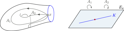
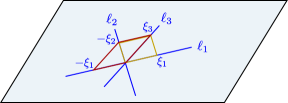
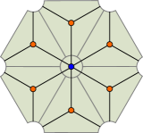
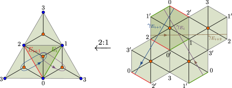
Now consider two invertible matrices . If , then there is a flat rank 2 complex vector bundle with holonomies about chosen based loops generating . Then—assuming each of is diagonalizable—there is a global abelianization based on the product double cover of . Our story begins when . In this situation the matrices determine a flat rank 2 complex vector bundle over the compact surface , as evoked by Figure 2. Let be a basepoint. There is no hope of a global abelianization. Instead, consider the ideal triangulation of depicted in Figure 3. If we collapse the boundary , there are 2 triangles, glued along 3 edges; each vertex is the point at “infinity” in . We interpret Figure 3 as a stratification
| (4.3) |
The codimension 2 stratum consists of two points, one interior to each face. The codimension 1 stratum is the union of six line segments, joining the codimension 2 stratum to the vertices. The generic stratum is the complement of the lower dimensional strata.
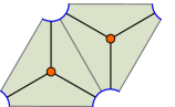
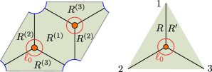
The first step in stratified abelianization is the choice of a parallel section of the associated projective bundle over , equivalently an eigenline of the commutator . The generic stratum has three contractible components, and for each the intersection has two contractible components; see Figure 4. By parallel transport from we obtain for each two parallel sections of . In the second drawing of Figure 4 the two sections in each component of are labeled by the two vertices in the closure of .
Assumption 4.4 (genericity).
For each , these sections are distinct.
Then, as in the 1-dimensional case, construct a global abelianization over the generic stratum:
| (4.5) | double cover | ||||
| (4.6) | flat line bundle | ||||
| (4.7) | isomorphism of flat bundles |
The map is the restriction of over the image of the two sections, and the line bundle (4.6) is the restriction of the tautological line bundle to . The genericity assumption allows us to construct (4.7) from the embedding .
As a preliminary, suppose are three distinct lines in a 2-dimensional vector space . Define
| (4.8) |
as the composition , where the second map is projection with kernel ; the composition is an isomorphism.
Our task is to extend the abelianization to a structure over the lower strata. Fix a component of and let be the components of on either side of . The intersection point picks out contiguous components of and . Glue the corresponding sheets of the double cover (4.5) along ; there is a distinguished sheet along from the contiguous components. In this manner extend (4.5) to a double cover
| (4.9) |
together with a section of over . Next, extend (4.6) to a flat line bundle
| (4.10) |
as follows. (We refer to Figure 4.) In passing from to , on the sheet obtained by parallel transport from vertex 1 glue via the identity. Cover the identification of the sheet 2 in and the sheet 3 in with the isomorphism (4.8) of the line bundle across the segment in .
We compare the isomorphisms (4.7) on each side of . By construction, the unipotent automorphism passing from region to region is
| (4.11) | ||||
Lemma 4.12.
Let be the link of and a component of .
Proof.
The proof of (i) is straightforward, so we omit it. For (ii), the holonomy about is the composition
| (4.13) |
Fix , and let , be the unique vectors such that . Then under (4.13) \incr@eqnum\mathdisplay@push\st@rredfalse\mathdisplayequation ξ_1⟼ξ_1⟼ξ_3⟼ξ_3⟼-ξ_2⟼-ξ_2⟼-ξ_1. ∎\endmathdisplayequation\mathdisplay@pop ∎
4.2. Stratifications, spectral networks, and abelianization
The double cover (4.9) together with the section over is called a spectral network (subordinate to the stratification (4.3)). Components of are the walls and is the branch locus. Notice that Lemma 4.12(i) implies that extends to a branched double cover with branch locus . The stratified abelianization of is the data:
In this subsection we give formal definitions of this structure which apply in some generality.
Two-dimensional spectral networks were introduced by Gaiotto-Moore-Neitzke [GMN1] in their study of supersymmetric 4-dimensional gauge theories. They have motivated many mathematical constructions and conjectures since, related to hyperkähler geometry, enumerative invariants, and asymptotic analysis of complex ODE, among others.
4.2.1. Stratifications
We use the definition [L, 4.3.2]. In that approach a type of stratified manifold of dimension is defined from the top down. Namely, begin with a geometric structure131313That is, a topological space equipped with a continuous map . An -manifold with an -structure is equipped with a lift of the classifying map of its tangent bundle. for the generic stratum in codimension 0. Then for each specify the geometric structure and link of a codimension stratum; the link is an -stratified -dimensional manifold. An -stratified manifold of dimension is built from the bottom up: first the highest codimension strata are specified, then higher strata with the proper link are glued in successively. This heuristic depiction is fleshed out precisely in [L, 4.3.2], and the heuristic specifications of the following definition can easily be formulated in that precise framework.
Definition 4.14.
An SN-stratification on a manifold-with-corners of dimension has the following specifications.
-
(i)
codimension 0: a codimension 0 smooth manifold;
-
(ii)
codimension 1: a codimension 1 submanifold—the link is a 0-sphere;
-
(iii)
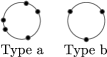
codimension 2: a Type141414Mnemonic: Type a is “anodyne”, Type b is “branch.” a codimension 2 stratum has link a circle with an arbitrary codimension 1 submanifold consisting of a finite set of points; a Type b codimension 2 stratum has link a circle with a codimension 1 submanifold consisting of 3 points;
-
(iv)
codimension 3: a Type a codimension 3 stratum has link a 2-sphere with an SN-stratification consisting of a codimension 1 trivalent graph whose vertices are of Type a; a Type b codimension 3 stratum has link a 2-sphere with the standard SN-stratification of the boundary of a tetrahedron (Construction 4.36 below).
We use the term SN-stratified manifold for a manifold equipped with an SN-stratification.
Remark 4.15.
There is a generalization of Definition 4.14 to manifolds with boundary and corners. The key point is that the SN-strata intersect boundaries and corners transversely.
In §§4.3, 4.4 we define canonical SN-stratifications associated to semi-ideal triangulations of 2- and 3-manifolds.
Remark 4.16.
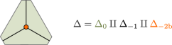
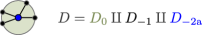
An SN-stratified manifold is decomposed as a disjoint union
| (4.17) |
where is the union of codimension 2 strata of Type a, is the union of codimension 2 strata of Type b, and likewise , are the unions of codimension 3 strata. This unusual notation is convenient for subsequent definitions: the Type a strata of codimension 2,3 behave as singular parts of the codimension 1 strata. Hence define
| (4.18) | ||||
4.2.2. Rank one Lie groups
Spectral networks and abelianization data are conveniently formalized in terms of a triple of complex Lie groups in which is a (complex) maximal torus of and its normalizer. In this paper we restrict to the groups , , and very occasionally . For we choose the subgroup of diagonal matrices; then its normalizer is
| (4.19) |
a 2-component Lie group with identity component . Choose the diagonal matrices to be the maximal torus of and its image in to be the maximal torus in the projective linear group; in each case the normalizer of has two components. Let be the subgroup
| (4.20) |
of upper triangular unipotent matrices. Then as well, and projects to a unipotent subgroup of .
Remark 4.21.
Each of the three groups acts on the projective line . In each case is the stabilizer subgroup of the 2-point subset of the axes in , and is the subgroup of elements of that act as the identity on . The stabilizer of the first axis is a Borel subgroup , and there is a diffeomorphism . Then for or , the Borel acts linearly on and , and is the subgroup of elements that act trivially on both and .
4.2.3. Definition of spectral networks and stratified abelianization data
Assume is one of the three triples defined in §4.2.2. We refer to it as the pair , since is determined as the normalizer of . Some notation: If is a principal -bundle, then we denote by its “inflation” to a principal -bundle. Also, if is a wall (a component), and is a principal -bundle, then there is an associated fiber bundle of groups
| (4.22) |
where acts on by conjugation.
The following definition applies to rank one groups, as does Definition 4.14; there are stratifications, spectral networks, and stratified abelianization data in higher rank as well [GMN1, GMN2, LP, IM].
Definition 4.23.
Let be a compact manifold of dimension with boundary. Suppose is equipped with an SN-stratification .
-
(i)
A spectral network subordinate to the stratification of is:
-
•
a double cover which restricts nontrivially to the link of each point in
-
•
a section of over
-
•
-
(ii)
Stratified abelianization data of type over is the data:
-
•
a principal -bundle with flat connection
-
•
a principal -bundle with flat connection
-
•
an isomorphism of double covers over
-
•
a flat isomorphism over
We require that the discontinuity of lie in as we cross a point of the wall .
-
•
Observe that the section reduces the restriction of over to a principal -bundle; on a wall the fiber bundle of groups is defined in (4.22). Stratified abelianization data over a given form a category; we leave to the reader the definition of the morphisms. Our usage of the term ‘spectral network’ often includes the underlying SN-stratification.
4.3. 2-dimensional spectral networks from triangulations
Let denote the standard affine plane. Denote the convex hull of a subset as . An affine triangle is the convex hull of three non-collinear points . Fix some , say . The truncated triangle is the convex hull of the six points for , as shown in Figure 7.

We will sometimes refer to “edges” or “vertices” of , meaning the corresponding edges or vertices of .
Let be the quotient of a finite union of disjoint truncated affine triangles whose edges are identified in pairs via affine isomorphisms. Then can be given the structure of a smooth compact 2-manifold with boundary.151515Indeed, since edges are identified in pairs, a neighborhood of any point on a glued edge is a disc; moreover the link of a vertex is easily seen to be a circle. The gluing of edges induces an equivalence relation on the vertices of the triangles ; each equivalence class of vertices corresponds to a boundary component of , with the topology of a circle. We sometimes call such an equivalence class a “glued vertex” or simply a “vertex”. Partition the glued vertices into two subsets of interior and ideal vertices. Let be a space obtained by gluing a copy of the standard disc to each boundary component of corresponding to an interior vertex. is a smooth compact 2-manifold with boundary; is canonically identified with the set of ideal vertices.
Definition 4.25.
Let be a compact 2-manifold with boundary. A semi-ideal triangulation of is a diffeomorphism , where is a space of the sort just described. The semi-ideal triangulation is called ideal if all vertices are ideal, and just a triangulation if all vertices are interior.
Construction 4.26 (SN-stratification of a truncated triangle).
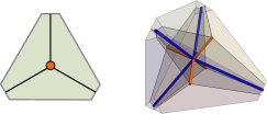
A truncated affine triangle carries a canonical SN-stratification as follows. Let be the barycenter of . Set ; the stratum is the union of the three line segments , ; and is the complement of . This SN-stratification is depicted in Figure 8.
Construction 4.27 (SN-stratification of the standard disc).
Let be the standard closed disc. For any finite subset we obtain an SN-stratification as follows. Let be the center of . Then ; is the union of line segments connecting to each point of ; and is the complement of . See Figure 9.
Construction 4.28 (SN-stratification of a triangulated surface).
Let be a closed 2-manifold equipped with a semi-ideal triangulation . Then transport of the SN-stratifications on the truncated triangles and the discs around interior vertices defines an SN-stratification of . Figure 3 is an example where there are no interior vertices. See Figure 10 for an example with an interior vertex.
Construction 4.29 (spectral network on a triangulated surface).
Let be the canonical SN-stratification of a truncated affine triangle (Figure 8). Each component of has boundary containing precisely one edge of , with two vertices. Let be the (trivializable) double cover whose fiber consists of those two vertices. Each component of is in the closure of two components of , with one vertex in common. Glue the corresponding sheets of the double cover to define together with a section over , i.e., a spectral network on . This construction glues across edges and extends to discs around interior vertices, and thus transports to give a spectral network over a semi-ideally triangulated surface .
Construction 4.30 (stratified abelianization data on a semi-ideally triangulated surface).
Consider first or . Assume that has no closed components and is equipped with a semi-ideal triangulation . Let be a flat principal -bundle. On each component of , choose a flat section of the associated -bundle , as in §4.1; see Remark 4.21 for the definition of the Borel subgroup . Also choose an element of the fiber of over each interior vertex. Use parallel transport—as in §4.1—to obtain two flat sections of . The following is a generalization of Genericity Assumption 4.4:
Assumption 4.31 (genericity).
The sections are nowhere equal.
Identify as a bundle of bases of a rank 2 complex vector bundle . The submanifold of bases contained in the lines defined by the sections determines a reduction of the principal -bundle to a principal -bundle . For , the limits of from the two sides of give three points in the projective line over . One of the sections has the same limit on both sides; the other has two possibly distinct limits. Let be the subgroup of elements which fix . Then is the projectivization of the 2-dimensional vector space , the group acts linearly on , and we define to be the unipotent element (4.11). Glue using at each to construct a flat principal -bundle . This gives most of the stratified abelianization data Definition 4.23(ii). We leave the rest to the reader, as do we the slight modifications for .
Remark 4.32.
The projection , defined via the isomorphism of double covers, is a principal -bundle. If or , then . If , there is an associated principal -bundle from the character of . Let be the associated flat line bundle. Lemma 4.12 holds in this more general situation.
We conclude with a theorem about stratified abelianizations over a single triangle equipped with the standard spectral network depicted in Figure 8. Specialize to and the corresponding subgroups . In this case there is a unique stratified abelianization, whose automorphism group is , in the following sense.
Proposition 4.33.
Let and be stratified abelianization data over . Then there is an isomorphism , unique up to composition with the simultaneous action of on and .
Proof.
First we construct a map of flat bundles . The monodromy of around lies in , since is the nontrivial double cover, and likewise for . But now recall that all elements of are conjugate in . It follows that there exists an isomorphism of flat -bundles, unique up to composition with an automorphism of .
The automorphism group of is the commutant of the monodromy, which is a cyclic group of order ; either generator acts nontrivially on , and the order element acts by . Thus, by composing with an automorphism of if necessary, we may arrange that , and the remaining freedom in is composition with the action of .
Next we construct a map of flat bundles . Along each wall we have a section of . On either side of the wall, then gives a section of ; the condition on the discontinuity of ensures that their projections to agree, thus giving a section of . Because acts simply transitively on triples of distinct points of , there exists which maps to for all three walls , and such a is unique up to a sign.
Finally we need to check that on we have (possibly after composing with the action of )
| (4.34) |
For this we consider the difference which is a covariantly constant section of , with two properties:
-
•
In a component of bounded by two walls , , the difference belongs to the subgroup preserving and . Thus acts by a constant scalar on , with .
-
•
The discontinuity of across belongs to the subgroup . It follows that is the same on both sides of .
Labeling the three walls as (with mod 3), the above properties say , which gives , so and thus . This completes the proof. ∎
4.4. 3-dimensional spectral networks from triangulations
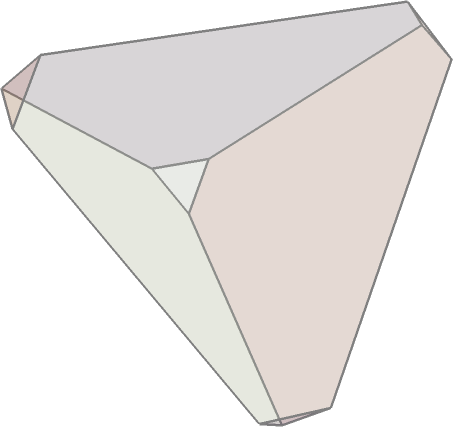
We begin with a 3-dimensional analog of Definition 4.25. A tetrahedron in is the convex hull of four points in general position. The truncated tetrahedron is the convex hull of the 12 points with . See Figure 11. We will sometimes refer to “faces”, “edges” or “vertices” of , meaning those of .
Let be the quotient of a finite union of disjoint affine truncated tetrahedra whose faces are identified in pairs via affine isomorphisms. Then can be given the structure of a smooth compact 3-manifold with boundary. The gluing of faces induces an equivalence relation on the vertices of the tetrahedra ; each equivalence class of vertices corresponds to a boundary component of , which is a compact connected surface. We sometimes call such an equivalence class a “glued vertex” or simply a “vertex”. Partition the glued vertices into two subsets of interior and ideal vertices, subject to the condition that the boundary component corresponding to an interior vertex must be diffeomorphic to . Let be a space obtained by gluing a copy of the standard 3-disc to each boundary component of corresponding to an interior vertex. is a smooth compact 3-manifold with boundary; is canonically identified with the set of ideal vertices.
Definition 4.35.
Let be a compact 3-manifold with boundary. A semi-ideal triangulation of is a diffeomorphism , where is a space of the sort just described. The semi-ideal triangulation is called ideal if all vertices are ideal, and just a triangulation if all vertices are interior.
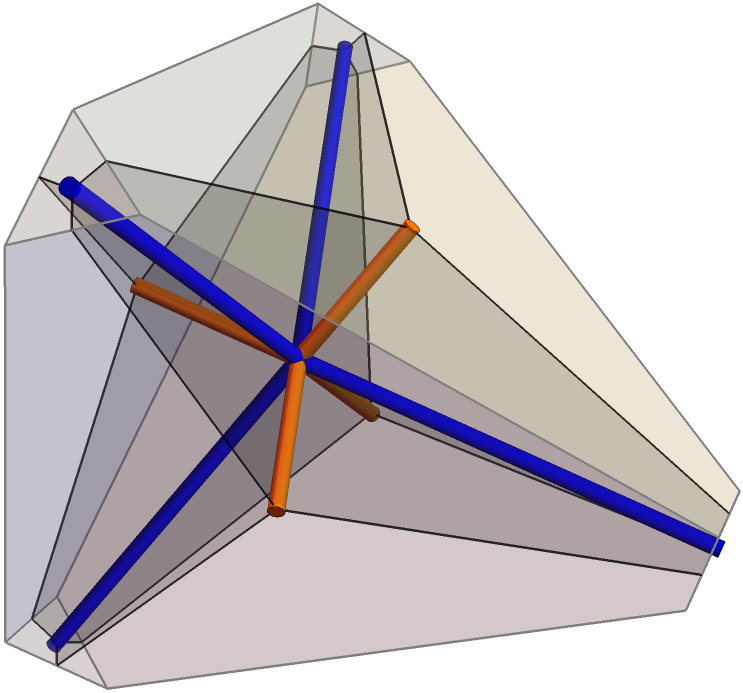
Construction 4.36 (Spectral network on a tetrahedron).
Let be a tetrahedron in . Let be the barycenter of the face opposite , ; set the barycenter of . (We use , .) Figure 12 depicts a canonical SN-stratification of ,
| (4.37) | ||||
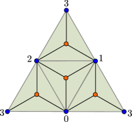
The link of is a 2-sphere triangulated as the boundary of a tetrahedron. By Construction 4.29 it has a canonical SN-stratification—the restriction of (4.37) to —and subordinate spectral network; see Figure 13. The same construction extends the SN-stratification to a 3-dimensional spectral network subordinate to (4.37). Namely, each component of contains one edge with two vertices, and each component of in corresponds to one of those vertices. Let be the (trivializable) double cover whose fiber over is the aforementioned set of two vertices, and glue along by identifying the common vertex on each wall. This produces a double cover with a section over , i.e., a spectral network. There is an extension to a branched double cover with branch locus .
Remark 4.38.
It will be convenient to excise an open ball about as well as its inverse image on the branched double cover.
We investigate stratified abelianization on the link of the barycenter of . The stratum of consists of 4 points, and the double cover extends to a branched double cover in which is diffeomorphic to a 2-torus. The double cover is depicted in Figure 14. The boundary of the tetrahedron has been unfolded, as in Figure 13, as has been the covering 2-torus. Assume is oriented, and use to induce an orientation on . To each edge in associate an element as follows. Let be a loop which crosses twice transversely and encircles the branch points in the faces of which abut . Orient as the boundary of the region which contains these two branch points. The desired lift is distinguished from the other lift of as follows: the lifts to of the two intersection points lie on the sheet of the double cover labeled by the closest endpoint of . Then is the homology class of in , the homology of the torus with the 4 branch points excised. Let be its image in the homology of the torus. We invite the reader to deduce the following, using Figure 14.
Proposition 4.39.
-
(1)
The image of under the deck transformation is .
-
(2)
Opposite edges of , such as 13 and 02 in the figure, induce the same homology class in .
-
(3)
The three pairs of opposite edges lead to three homology classes which sum to zero.
Cyclically order the three pairs of opposite edges so that the intersection product for . Denote the corresponding loops in as .
Let be the set of 4 branch points . Since is simply connected, any flat -bundle is trivializable. Fix in the fiber of the associated -bundle at each vertex . Let be the space of horizontal sections of , and let be the extension of the previous to a horizontal section. Assume that are distinct; this implies the Genericity Assumption 4.31. Use Construction 4.30 to produce a stratified abelianization. By Remark 4.32 there is a flat line bundle
| (4.40) |
with holonomy around each of the 4 (branch) points in . The isomorphism class of the flat bundle (4.40) is determined by its holonomy, a homomorphism
| (4.41) |
Set for .
Proposition 4.42.
The holonomies of satisfy
| (4.43) |
Proof.
We compute as in the proof of Lemma 4.12 using Figure 14 as a guide. The holonomy of around is the composition
| (4.44) |
and the holonomy of around is the composition
| (4.45) |
(Recall the projections in (4.8).) Choose , and then , such that
| (4.46) | ||||
for some . Then and , etc. Hence the image of under (4.44) is , and the image of under (4.45) is . Therefore, \incr@eqnum\mathdisplay@push\st@rredfalse\mathdisplayequation z _i+1=hol^_L(λ^_E_i+1)=1-1z = 1-1holL(λEi) = 1 - 1z i. ∎\endmathdisplayequation\mathdisplay@pop ∎
Remark 4.47.
-
(1)
One interpretation of is as follows. Recall that 4 distinct points in a projective line are characterized up to isomorphism by their cross-ratio. If are the corresponding lines in the 2-dimensional vector space , then the cross-ratio is
(4.48) where the numerator and denominator are nonzero elements in ; the ratio is independent of the choice of . Permuting the lines we obtain numbers , , , , , for some . In the case at hand, with the chosen vectors in (4.46), we compute
(4.49) -
(2)
As a corollary of Proposition 4.42 the product of the holonomies around the loops defined after Proposition 4.39 is
(4.50) This leads to a sharpening of Proposition 4.39(3). Let be a link of the 4 points , so is a union of 4 disjoint circles , one surrounding each branch point. Form the commutative diagram
(4.51) in which the homomorphism maps a generator of to . The bottom row of (4.51) is a central group extension. The refinement of Proposition 4.39(3) is that the product of the images of in is .
-
(3)
The space is the domain of the real dilogarithm function (2.1), and the total space of an abelian cover is the domain of the enhanced Rogers dilogarithm (2.9). In our current setup is a space of flat -connections on a punctured torus. In §7.2 we introduce an extra twist to get rid of the punctures, and so identify as a space of flat -connections on a torus. See [FN] for a development of the dilogarithm function with this starting point.
Construction 4.52 (SN-stratification on a 3-disc).
Let be the standard closed 3-disc. Given an SN-stratification of the boundary , of the form , we obtain an SN-stratification of as follows. Let be the center of . Then , , and each other stratum is the cone over with removed.
Construction 4.53 (Stratified abelianization data on a 3-manifold).
Let be a compact 3-manifold with boundary, and suppose is a semi-ideal triangulation. The SN-stratification (4.37) and subordinate spectral network on each truncated tetrahedron transport to , and extend over the 3-discs around interior vertices. In particular, there is a branched double cover with branch locus .
Suppose is a flat principal -bundle. Assume there exists161616Existence condition: on each component of the holonomies around loops at a basepoint have a common eigenline. a flat section of the restriction of the associated -bundle to , and furthermore that we can and do choose a section such that Genericity Assumption 4.31 hold. Excise from open balls about the barycenters of the tetrahedra. Let be the total space of the double cover with the inverse images of the balls excised. Then is a compact manifold with boundary , where each is a 2-torus. The preceding gives an SN-stratification of with strata of codimension 0, 1, and 2, and a flat line bundle . The holonomy around a circle linking is .
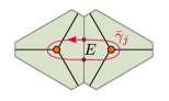
Remark 4.54 (Thurston gluing equations).
Each tetrahedron in Construction 4.53 has a shape parameter which is one of the holonomies defined before Proposition 4.42. (There are three possibilities labeled by the three pairs of opposite edges of .) Let be an edge in the triangulation , and let be the set of such that is an edge of . For , let be the loop in the torus which is called ‘’ in the text following Remark 4.38. Then
| (4.55) |
To prove this relation consider Figure 15. Depicted are the two faces of , , which abut and the image of the corresponding loop . Now each of the triangular faces occurs in exactly one additional tetrahedron , , and it does so with the opposite orientation. Hence the halves of and contained in that face cancel, as do the halves of their lifts and . This leads to (4.55). (The cancellation is in homology; the actual half curves are not strictly opposite.) The relation (4.55) in homology immediately implies the Thurston gluing equation [T2, §4.2]
| (4.56) |
where we choose the edge to define the shape parameter in each , .
5. Levels and Chern-Simons invariants
We begin in §5.1 by proving relations among the Chern-Simons levels of , , and their various subgroups. This is the topological basis for abelianization. These topological computations imply relations among secondary differential geometric invariants via differential cohomology. We provide a brief introduction to differential cohomology in Appendix A. In §5.2 we introduce the spin refinement of Chern-Simons theory and prove appropriate relations among the “spin levels”. We fully embrace differential cohomology in §5.3, where we prove a key result: Theorem 5.59. It states, heuristically, that moving in the unipotent direction does not change Chern-Simons invariants. We also prove results about Chern-Simons theory (Theorem 5.81, Corollary 5.87, Corollary 5.101) that are important in our later work. We conclude with a global statement, Theorem 5.104, of abelianization. Our main focus, stratified abelianization, is the subject of the subsequent §§6–8.
In this section we change notation slightly. Set and let be the subgroups defined in §4.2.2. Also, set and let be the associated subgroups; the unipotent subgroup is a subgroup of , hence too of .
We remind of a choice made in Example 3.7.
Convention 5.1.
3-dimensional Chern-Simons theory is based on the level .
In that section the level is encoded in a symmetric bilinear form (3.1) on the Lie algebra, and (3.8) is the form that corresponds to . In the next section we compute the restriction of to the subgroup , and then we will define Chern-Simons theory on —or, rather, a spin refinement—in terms of that restricted level.
5.1. Levels and abelianization
5.1.1. Levels in
Our goal is to relate Chern-Simons invariants of principal -bundles to Chern-Simons invariants of -, -, and -bundles, and to do the same for -bundles. These derive from relationships among appropriate degree four integral cohomology classes on the classifying spaces, which we prove in this section. The inclusions and surjective homomorphism lead to a diagram
| (5.2) |
in which is a double cover and the vertical maps form a fibration sequence. The section of is the classifying map of the inclusion . Let , , be the universal Chern classes, and the universal first Pontrjagin class. Let be the first Chern class of the homomorphisms indicated by the matrix . Let be the generator; note .
Proposition 5.3.
In diagram (5.2) we have the following equality in :
| (5.4) |
Proof of Proposition 5.3.
From the Leray-Serre spectral sequence of the vertical fibration in (5.2), we deduce the split short exact sequence171717It helps to observe that the action of on exchanges the two summands, so the resulting local system on is the pushforward of the trivial local system on its contractible double cover. Hence the cohomology vanishes in positive degrees.
| (5.5) |
Hence a class in is determined by its pullbacks under and .
For the deck transformation, we have . Hence
| (5.6) |
because are the Chern roots of the universal -bundle. Since induces an isomorphism on , the fiber product of and is contractible, from which . Also, , since is torsion of order two. The composition classifies the sum of the complex sign and trivial representations of , so its first Chern class is the generator . Combining the preceding with we deduce (5.4). ∎
Remark 5.7.
For a level is parametrized by integers . By a similar argument to the preceding proof, , from which
| (5.8) |
Thus we can realize any level with even by a linear combination of and , up to .
5.1.2. Levels in
By restriction we deduce a formula for the “special” subgroups which appear in the diagram
| (5.9) |
Lemma 5.10.
In the diagram (5.9) we have .
Proof.
Let be the generator. Then , where is the integral Bockstein, and also . It suffices to prove . Passing to maximal compact subgroups we replace by . In the Leray-Serre spectral sequence for the fibration sequence , the differential sends the generator to . (See [KT] for a review of pin groups.) Then . Also, since transgresses so too do its Steenrod squares, and in particular . Hence is killed when pulled back to . Conclude by observing that
| (5.11) |
commutes. So the pullback of equals the pullback of . ∎
The classifying map of the inclusion satisfies for a generator. Also, . The following is a corollary of Proposition 5.3 and Lemma 5.10.
Corollary 5.12.
In diagram (5.9) we have the following equality in : \incr@eqnum\mathdisplay@push\st@rredfalse\mathdisplayequation p_*c^2 = -2r^*c_2. ∎\endmathdisplayequation\mathdisplay@pop
5.1.3. Abelianization of connections
Let us now focus on . If is a 3-manifold with a flat -connection, then global abelianization of the associated flat -connection is encoded in the commutative diagram
| (5.14) |
where we write for the group of diagonal matrices . The pullback square defines the (unramified) double cover . Stratified abelianization is encoded in the diagram
| (5.15) |
in which the bottom triangle commutes on . In both the global and stratified cases our goal is to compute the Chern-Simons invariant of the flat -connection on in terms of a Chern-Simons invariant of the flat -connection on . The Chern-Simons invariant is the secondary invariant of ; the Chern-Simons invariant is the secondary invariant of . There is a mismatch for abelianization: the factor of in (5.12). To rectify we must divide the -level by 2 (and include the minus sign). This can be done—a secondary invariant for “” exists—but at the cost of introducing a new cohomology theory and a spin structure on , as we explain in §5.2.
Remark 5.16.
Levels have a refinement in differential cohomology, and the Chern-Simons invariants are nicely located in the differential theory; see [ChS, HS, F2, FH2]. We give a précis of differential cochains in Appendix A and use this point of view on Chern-Simons invariants in §5.3; see also [FN, Appendix A]. This framework makes clear that cohomology identities immediately imply corresponding relations among secondary invariants.
We conclude our discussion of levels in ordinary cohomology by examining the restriction to the unipotent subgroup in (4.20). Recall (Definition 4.23(ii)) that the failure of the bottom triangle in (5.15) to commute on all of is due to the unipotent gluing along the walls (components of ) of the spectral network. Since is contractible, so is , and the following is immediate.
Proposition 5.17.
The restriction of any level of or to vanishes. ∎
5.2. Levels for spin Chern-Simons theory
5.2.1. -cohomology and spin Chern-Simons theory
To divide by 2, we pass to a cohomology theory simply denoted , the nontrivial extension
| (5.18) |
of Eilenberg-MacLane spectra; the -invariant is , the composition of the integral Bockstein and the Steenrod square. For any topological space , the extension (5.18) leads to a long exact sequence of cohomology groups
| (5.19) |
Multiplication by 2 on factors through :
| (5.20) |
For , a slice of the long exact sequence (5.19) is the nontrivial abelian group extension
| (5.21) |
i.e., is infinite cyclic and is twice a generator . The class plays the role of “”. Passing to maximal compact subgroups there is a generalization from to for any . Namely, there is a characteristic class whose image under is . Furthermore, is additive: for real vector bundles over a space we have
| (5.22) |
The pullback of to is the image under of a class whose double is . Also, if . We refer to [F3, §1] for background about this cohomology theory and proofs181818Even if the precise statement does not appear in [F3], the same techniques apply. The standard fact that follows since and is a generator, if . of these assertions.
The characteristic class has a lift to the differential -cohomology of the classifying object for principal -connections. (See [FN, Appendix A].) Here is a simplicial sheaf on smooth manifolds, in the sense of [FH2], for example. There is also a simplicial sheaf which classifies flat -connections, as well as a map . The pullback is a flat differential class. Define the spectrum as the cofiber of the composition
| (5.23) |
Its nonzero homotopy groups are and . The topological space is a geometric realization of the simplicial sheaf . Then determines a characteristic class
| (5.24) |
in the cohomology theory .
An oriented real vector bundle has a Thom class in integer cohomology, but a Thom class in -cohomology requires a spin structure [F3, Proposition 4.4]. In particular, -cohomology classes can be integrated on compact spin manifolds. This leads immediately to a fully extended unitary 3-dimensional topological field theory on spin manifolds equipped with a flat -connection, analogous to the usual Chern-Simons theory (3.12) on oriented manifolds. It has a fully local version defined as a map of spectra analogous to (3.13):
| (5.25) |
The field theory (5.25) assigns a -graded line to a closed spin 2-manifold with flat -connection. As noted in Remark 3.14 we need the theory for parametrized families of flat connections, so for nonflat connections.
Remark 5.26.
In fact, the grading of the spin Chern-Simons line of a -connection on a surface is determined by the parity of the degree of the underlying principal -bundle. For a flat connection that degree is zero, hence the line is even. Also, to a -connection over a spin 1-manifold, the spin Chern-Simons theory assigns an invertible module over super vector spaces. See Appendix C for more details as well as a justification for ignoring these -gradings in the body of this paper.
As a companion to Convention 5.1 we signpost our choice of sign for the level, which is motivated by Corollary 5.39 below.
Convention 5.27.
3-dimensional spin Chern-Simons theory is based on the level .
This spin Chern-Simons theory is developed in some detail in [FN]. For future use we recall one particular result: [FN, Theorem 3.9(vii)]. Let be a closed 2-manifold endowed with a spin structure , and fix a principal -bundle with connection . A section of produces
| (5.28) |
a nonzero element in the spin Chern-Simons line computed from the -connection and the spin structure . Let be a smooth function. Then is another section of , and the ratio of nonzero elements in is
| (5.29) |
where
| (5.30) |
Here is the quadratic refinement of the intersection pairing given by the spin structure , and is the reduction modulo two of the homotopy class of .
5.2.2. Levels in -cohomology
We revisit Proposition 5.3 and Corollary 5.12 in -cohomology, so effectively divide (5.4) and (5.12) by 2.
Lemma 5.31.
-
(1)
The map
(5.32) is an isomorphism.
-
(2)
The group extension
(5.33) is nontrivial: is cyclic of order 4.
-
(3)
The pullback map is zero.
Proof.
Statement (1) follows from . For (2), we claim
| (5.34) |
has order 4, where is the real Hopf line bundle. For this observe is orientable, , and since and , so . (We use the Whitney sum formula (5.22).) Finally, (3) follows immediately from . ∎
Observe that , where is the generator.
Remark 5.35.
Let be the homomorphism . Observe that the pullback vanishes, since and . The Chern-Simons theory based on defines invariants of compact oriented manifolds equipped with a double cover. A lift of a double cover to a principal -bundle trivializes191919The Chern-Simons theory is defined using a geometric representative of , say a map , where is the 4-space in the spectrum , sometimes denoted . The trivialization is based on a choice of null homotopy of the composition . the Chern-Simons invariant.
Let be the pullback of the generator under , where ; then . Let be the unique class such that . (See (5.20) for the definition of .) Identify with its image under in .
Proposition 5.36.
In diagram (5.2) we have the following equality in :
| (5.37) |
Proof.
In the diagram
| (5.38) |
the rows are exact, and the first and third columns are exact; see (5.5). It follows that the second column is also exact. In other words, a class in is determined by its pullbacks under and . Also, observe that twice (5.37) is (5.4), which implies that the two sides of (5.37) differ by an element of order dividing 2. Since is torsionfree, as can be deduced from (5.21), it follows that the pullback under of the two sides of (5.37) agree. For the pullback under we argue as in the proof of Proposition 5.3: the -class of the complex sign representation is ; see (5.34). ∎
Corollary 5.39.
In diagram (5.9) we have the following equality in : \incr@eqnum\mathdisplay@push\st@rredfalse\mathdisplayequation p_*λ=-r^*c_2 + q^*α. ∎\endmathdisplayequation\mathdisplay@pop
5.3. Chern-Simons theory and differential cochains
Shortly after the introduction of secondary invariants of connections by Chern-Simons [CS2], Cheeger-Simons [ChS] recast them in terms of new objects in differential geometry: differential characters. Differential cohomology, which we discuss briefly in Appendix A, introduces cochains into the theory of differential characters; it is the natural home in which to express the full locality of Chern-Simons invariants. In [FN, Appendix A] we prove some properties of spin Chern-Simons theory using generalized differential cohomology, and in §5.3.5 we take this up to prove a lemma we need later. Otherwise, in this section we restrict to ordinary differential cohomology with complex coefficients and Chern-Simons theory for . Our main goal is to prove Theorem 5.59 about the behavior of Chern-Simons invariants under unipotent modifications. We begin with some preliminaries in §§5.3.1–5.3.3. A global abelianization theorem appears in §5.3.6.
5.3.1. The universal -connection
Let be a Lie group with finitely many components. There is a groupoid-valued sheaf on the category of smooth manifolds whose value on a test manifold is the groupoid of -connections; see [FH2] for an introduction and details. The sheaf classifies -connections: there is a universal principal -bundle
| (5.40) |
with connection , and if is a principal -bundle with connection over a smooth manifold , then there is a unique -equivariant map which satisfies . Moreover, the universal connection on (5.40) is a weak equivalence
| (5.41) |
where is the set-valued sheaf which assigns to a test manifold the set of -valued 1-forms on . The total space of (5.40) assigns to the discrete groupoid of principal -bundles with connection and section ; the universal connection (5.41) maps the triple to the -valued 1-form .
The universal Chern-Simons-Weil invariant is a differential cohomology class on . The variant of differential cohomology we need uses complex differential forms. The construction of as a homotopy fiber product [HS, BNV, ADH] leads to the exact sequence
| (5.42) |
in which denotes the vector space of closed complex differential forms. The main theorem of [FH2] computes as the vector space of real linear -invariant symmetric bilinear forms . For we choose and the bilinear form
| (5.43) |
as in Example 3.7; see also Convention 5.1. By (5.42) there is a unique lift , the desired universal Chern-Simons-Weil class. This gives, for each principal bundle with connection over a smooth manifold , a differential characteristic class . We need a refinement to a differential cocycle representative of this class in ; see §A.1. This depends on a contractible choice; see [F2, §3.1] or [HS, §3.3] for detailed constructions. We use the same symbol for the differential cocycle representative, and make clear whether it denotes the cocycle or cohomology class.
Suppose is an iterated fiber bundle in which is a principal -bundle and the fibers of are manifolds with boundary of dimension . Assume given an orientation on , i.e., on the relative tangent bundle . Let be a connection. We obtain a differential cocycle . The Chern-Simons invariant of this family of -connections is
| (5.44) |
a differential cochain in ; see §A.4 for the integral. For and assuming the fibers of are closed, (5.44) is a function , as in (3.4). For and closed fibers (5.44) is a complex line bundle with covariant derivative over , the Chern-Simons line bundle. For and a fiber bundle of manifold with boundary, (5.44) is a section of the Chern-Simons line bundle computed from the boundaries; see Theorem A.24.
Consider the pullback to the total space of the universal bundle (5.40). Let denote the presheaf of closed differential forms with integral periods. The exact sequence
| (5.45) |
from [HS, (3.3)] reduces to an isomorphism (the middle map), since . Hence reduces to a 3-form modulo closed 3-forms with integral periods. There is a canonical choice of 3-form,202020Use (A.10) to deduce the existence of this 3-form. the Chern-Simons form ; see (3.2). To a triple which represents a map , the pullback of to is
| (5.46) |
where . The Chern-Simons invariant of an oriented family with connection and trivialization can be computed by integrating the 3-form (5.46) over the fibers of . For example, if the fibers of are closed of dimension 2, then the resulting 1-form on is the connection form of a trivialized complex line bundle over .
5.3.2. Restriction to the unipotent subgroup
Recall the unipotent subgroup defined in (4.20).
Definition 5.47.
Let be a smooth manifold with boundary.
-
(1)
A flat principal -bundle is boundary-unipotent if its restriction to the boundary admits a reduction to a flat principal -bundle.
-
(2)
Such a is boundary-reduced if a reduction is chosen.
-
(3)
Stratified abelianization data over is boundary-reduced if is boundary-reduced and lies in the -bundle given by the reduction.
Note that a flat -bundle is boundary-unipotent iff on each boundary component the holonomies around loops at a basepoint have a common eigenline. Moreover, if is boundary-reduced, then is a trivializable flat bundle, since .
Let be the groupoid-valued sheaf of -connections. Then there is a map .
Lemma 5.48.
The restriction of the universal second differential Chern class to vanishes.
Proof.
Since is contractible, the restriction of to vanishes; also, the restriction of the bilinear form (5.43) to the Lie algebra of vanishes. ∎
Recall that we choose a differential cocycle representative of ; see the text following (5.43). Now choose a trivialization of its restriction to .
Remark 5.49.
With these choices, the Chern-Simons invariant of a boundary-reduced flat -bundle is trivialized on the boundary. For example, on a compact 2-manifold with boundary, the invariant is a complex line.
5.3.3. A lemma in differential cohomology
Let be an oriented -manifold with corners, equipped with the extra structure of a bordism outlined in §A.4; let be a smooth manifold, which plays the role of parameter space; and suppose212121 has the structure of a bordism: set (5.50) is a differential cocycle of some degree . Let be the “curvature” of , i.e., the differential form underlying the differential cocycle . Let denote the standard vector field on , lifted to , and let denote its action via contraction on differential forms. Theorem A.24 implies the following for closed.
Lemma 5.51.
If is closed, then the integral
| (5.52) |
is a nonflat isomorphism of the differential cocycles on computed in the domain and codomain. Its covariant derivative is
| (5.53) |
In particular, if , then (5.52) is a flat isomorphism. ∎
If is a manifold with corners—a bordism of positive depth—then the integrals of over and are higher morphisms in a groupoid of differential cochains on : see §A.3. For example, if has depth , then the integrals are 2-morphisms in , as depicted in (A.27).
Lemma 5.54.
We omit the integrand ‘’ in (5.55) for readability.
Example 5.56.
Example 5.57.
If and , then (5.53) reduces to a well-known formula for the ratio of holonomies of a line bundle with connection around the ends of a cylinder.
5.3.4. Moving along unipotents
Theorem 5.59 below is based on the fact that the bilinear form (5.43) vanishes if is diagonal and is upper triangular.
Let be an oriented manifold with corners of depth and dimension . Suppose is equipped with an SN-stratification which satisfies . In other words, . Suppose is a subordinate spectral network. Thus is a double cover and is a section of over . Let denote the diagonal subgroup, and its normalizer. Suppose is stratified abelianization data of type . Thus
-
(1)
is a principal -bundle with flat connection ,
-
(2)
is a principal -bundle with flat connection ,
-
(3)
is an isomorphism of double covers, and
-
(4)
is an isomorphism of flat principal -bundles over .
Furthermore, let be the subgroup (4.20) of unipotent matrices. Then we require that the discontinuity of along lie in , relative to the reduction of to a principal -bundle given by the section .
Our task is to compute the Chern-Simons invariants (5.44) of the flat -bundles and . To state the theorem we posit a family of this data over a smooth manifold . Thus we work over ; the connections over are only assumed flat along .
Theorem 5.59.
There is a natural flat isomorphism
| (5.60) |
Intuitively, moving a connection in unipotent directions does not affect the Chern-Simons invariant. In the proof we construct a flat isomorphism which depends on a set of choices, and then we check that the isomorphism is independent of the choices.
Proof.
Fix a smooth function which is odd and satisfies
| (5.61) |
Furthermore, require that be monotonic nonincreasing on and . Choose a tubular neighborhood of : an open subset which contains , a surjective submersion , and an isomorphism of with the normal bundle to . (See Figure 16.) Fix an inner product on . Let be the reduction of to a principal -bundle; it is defined via the section and isomorphism . Locally, for each orientation of the discontinuity in along is a section of the bundle of unipotent groups. Under reversal of orientation, maps to . Globally, write for a section of the bundle of Lie algebras
| (5.62) |
twisted by the orientation bundle of . Extend to using parallel transport along the fibers of . The inner product on the normal bundle identifies each fiber of with after choosing an orientation of the normal bundle. Hence the product is a well-defined section of the pullback of (5.62) over . It extends222222Since the codomain of does not so extend, this is not strictly correct. What we mean simply is that in formulas below replace by ‘0’ on . by zero to .
We now construct a connection on the principal -bundle
| (5.63) |
whose restriction to is isomorphic to and whose restriction to is isomorphic to . First, set . Then over let be the gauge transformation of the restriction of (5.63) which equals on and is the identity map on . Construct an isomorphism
| (5.64) |
which equals on ; it extends over using the fact that jumps by on . Set . Finally, define on by affine interpolation between the specified connections :
| (5.65) |
Then is a 1-form on with values in the adjoint bundle of Lie algebras isomorphic to ; it has support on . We claim that takes values in the subbundle (5.62) of nilpotent subalgebras, extended over by parallel transport along the fibers of . Namely, on we have
| (5.66) |
The second term clearly lies in the nilpotent subalgebra. For the first, observe
| (5.67) |
is nilpotent.
Let be the Chern-Simons-Weil differential cocycle. As in (5.55),
| (5.68) |
is an isomorphism. We claim that it is a flat isomorphism. By Lemma 5.54 it suffices to show that , where
| (5.69) |
is the Chern-Weil 4-form of . The only nonzero contribution to is potentially on . From (5.65) we compute the curvature
| (5.70) |
The last term vanishes since the Lie algebra of the unipotent group is abelian. The first term in (5.70) takes values in the diagonal subalgebra and the other terms take values in the nilpotent subalgebra . It follows that
| (5.71) |
It remains to prove that (5.68) is independent of the choices of and the isomorphism of with the normal bundle. Any two sets of choices can be joined by a path, so we extend the previous setup by taking the Cartesian product with . If is the resulting Chern-Weil 4-form, then by a similar argument. ∎
5.3.5. A theorem in Chern-Simons theory
Recall from §5.2.1 and [FN, Appendix A] the characteristic class and its differential refinement , the universal differential class. The class is the image of the generator under a quadratic function
| (5.72) |
which for satisfy
| (5.73) | ||||
| (5.74) | ||||
| (5.75) |
where and are the maps in (5.18), and we denote . The differential refinement
| (5.76) |
satisfies analogous properties. We implicitly use refinements of to cochains. Recall that integration232323In (5.77) we also use the integral symbol for the pairing of a mod 2 cohomology class with the fundamental class. of -cocycles over a manifold requires a spin structure on . Furthermore, if is the class of a double cover over , and we write the shifted spin structure as242424Our notation conflates a double cover and its equivalence class, an overload we also deploy in this section for spin structures and -connections. , then
| (5.77) |
where ; see [F3, Proposition 4.4] and [FN, Theorem 3.9 (ii)]. For and closed, (5.77) is an equation in ; for manifolds with boundary and manifolds of lower dimension it is a canonical isomorphism of cochains in -cohomology theory. We use the differential refinement of (5.77).
Not only do double covers shift spin structures, but they also shift -bundles via the homomorphism . The corresponding shift of Chern classes is via the integer Bockstein
| (5.78) |
The differential refinement shifts -connections by a flat -connection of order two.
The following is a restatement of part of Lemma 5.31.
Lemma 5.79.
with generator for the nonzero class. Also, is the image of under the map .
Proof.
Our main result in this section expresses the change of spin Chern-Simons invariants under the simultaneous shift of spin structure and -connection by a double cover. We express our result as a relation among 3-dimensional invertible field theories whose background fields are independent choices of: a spin structure , a double cover , and a -connection . The partition functions which define the theories are:
| (5.80) | ||||
The theory is topological (of order 4). The Chern-Simons invariants in are based on , and so are computed by integrating , the quadratic function (5.72).
The proofs in the rest of this section draw on the material in Appendix B.
Theorem 5.81.
There is an isomorphism of invertible field theories.
Proof.
By (B.12) the curvatures of and are equal. Therefore is a flat invertible field theory, so it is topological in the strong sense. To verify that it is trivializable, it suffices to check the partition function on a closed 3-manifold . The quadratic property (5.75) implies
| (5.82) |
and (5.77) implies that its integral in spin structure is the integral of
| (5.83) |
in spin structure . Here is the inclusion of flat elements of order two. (The first two terms of (5.83) lie in and their integral uses the spin structure; the last two terms lie in and no spin structure is used to integrate.) The difference of and (5.83) computes the partition function in the theory :
| (5.84) | ||||
where we use Lemma 5.79. Since the integral of this last quantity is by definition the partition function in the theory , we see that the partition function in the theory is trivial. ∎
Example 5.85.
Let equipped with either spin structure and the nontrivial double cover . The spin Chern-Simons partition function of the product -connection is 1; the partition function of the -connection in either spin structure is a primitive root of unity.
A principal -bundle has a mod 2 reduction which is a double cover. The invertible field theories in (5.80) lift to invertible field theories with background fields .
Theorem 5.86.
is isomorphic to the trivial theory.
Proof.
The integer Bockstein of the mod 2 reduction is trivial. ∎
Corollary 5.87.
There exist isomorphisms .
For our work in §6 we need an isomorphism which satisfies a particular property that we specify below in (5.100). We proceed to construct it. To begin, fix a flat252525Isomorphisms of invertible field theories may be flat or nonflat; compare §A.2. isomorphism
| (5.88) |
Pull back the theories to invertible theories with background fields in which is a nonflat trivialization of the -connection , i.e., is a section of the underlying principal -bundle. Then induces a nonflat trivialization of the theories : they are topologically trivial. In the formalism of Appendix B we omit the spin structure, and the remaining fields are sections of the sheaf262626A principal -bundle has a unique connection, so the ‘’ in ‘’ is redundant; the latter is better denoted ‘’ on . It is convenient to replace with the representable sheaf . This amounts to specifying a classifying map for each principal -bundle. Then the topologically trivialized theories , , give rise to differential forms (see (B.9))
| (5.89) |
Let be the rotation-invariant closed 1-form which integrates to , and let be times the universal connection 1-form; the latter gives the equivalence . Then from (5.73) we deduce
| (5.90) | ||||
The topologically trivialized theories defined by are isomorphic as invertible theories (forgetting the topological trivialization)—as they must be by Corollary 5.87—since the 3-forms differ by an exact 3-form.
Our constructions yield two isomorphisms . First, the flat isomorphism lifts to a flat isomorphism
| (5.91) |
Second, the topological trivializations induce a nonflat isomorphism
| (5.92) |
From (5.90) we compute that the curvature of is . The ratio is a 2-dimensional invertible theory on spin manifolds with a background field in , and its curvature is the 3-form . Let be the 2-dimensional invertible field theory defined by the 2-form
| (5.93) |
and define the flat 2-dimensional theory by
| (5.94) |
Lemma 5.95.
The abelian group of topological invertible 2-dimensional theories with background fields is isomorphic to the Klein group . Furthermore, each theory depends only on the spin structure and the double cover induced by the principal -bundle .
The partition functions of these four theories on a closed 2-manifold are
| (5.96) |
where is the Arf invariant of the spin structure.
Proof.
Since is contractible, the group of invertible theories is isomorphic272727Both unitary and nonunitary theories are discussed in [FH1]. Here we do not assume unitarity, but the background fields are for 3-manifolds, even for the 2-dimensional theory which is the ratio of isomorphisms of 3-dimensional theories, hence the domain should at first glance have in place of . However, the obstruction theory argument in the proof of [FH1, Theorem 7.22] allow us to replace with in (5.98). to the group of characters of
| (5.97) |
One can see that the theories listed in (5.96) exhaust the possibilities, or can check that
| (5.98) |
induces an isomorphism on . ∎
It follows that the theory in (5.94) depends only on . Therefore, replace (5.88) by the isomorphism
| (5.99) |
For this choice of isomorphism we have
| (5.100) |
where recall that is defined by the 2-form (5.93).
We summarize with this refinement of Corollary 5.87.
Corollary 5.101.
This is the isomorphism we use in §6.
5.3.6. Global abelianization
Diagram (5.14) illustrates global abelianization of an -connection. We apply Corollary 5.39 to deduce an isomorphism of Chern-Simons invariants, expressed as an isomorphism among three invertible 3-dimensional field theories282828As in Theorem 5.81 we restrict to flat connections, so to topological invertible field theories. , , and . Each is defined on the bordism multicategory of dimension manifolds with corners equipped with a spin structure and a flat -connection . The first theory uses only the underlying orientation of , and it evaluates the Chern-Simons theory at level on the flat -connection . The second theory maps a spin manifold with flat -connection to the total space of the associated -bundle with its induced spin structure and flat -connection, and then evaluates this data using spin Chern-Simons theory at level . The third theory evaluates the spin Chern-Simons theory at level on the associated -connection292929Of course, this is simply a double cover, but we have endeavored to use consistent and transparent notation. .
Theorem 5.104.
There is an isomorphism .
Proof.
Let denote the pullbacks of to the bordism multicategory of dimension manifolds with corners equipped with a spin structure, a flat -connection, and a lift of the associated -bundle to a principal -bundle. Then Lemma 5.31(3) immediately implies
Theorem 5.106.
is isomorphic to the trivial theory.
Corollary 5.107.
A trivialization of determines an isomorphism .
6. Abelianization of Chern-Simons lines
Throughout this section we take .
So far we have discussed generalities about the Chern-Simons theories , , and their relation to one another via stratified abelianization. Now we begin discussing applications.
Suppose is a compact 2-manifold, equipped with a boundary-reduced flat -bundle . In this section and the next we give a new description of the line . The idea is to identify with , where is a flat -bundle over a branched double cover , and is a universal line which does not depend on . In the rest of this section we give a sketch of the construction.
The bundle will be constructed as follows. First, we fix a semi-ideal triangulation of , and let be the associated branched double cover, and the associated spectral network (Construction 4.29). Next, we fix a section of over each vertex of (as usual, for ideal vertices this means a flat section over the corresponding boundary component), obeying the genericity Assumption 4.31. From these data, by Construction 4.30 we obtain stratified abelianization data .
Now, suppose we ignore the branch locus for a moment, i.e. we work just over . Then, according to Theorem 5.59, is naturally isomorphic to ; and by Corollary 5.107, if we choose a spin structure on , and a lift of to a -bundle , is naturally isomorphic to . Composing these two we would get an isomorphism
| (6.1) |
This is the kind of statement we are after, but to extend the right side over the full it needs to be modified. The complication is that has holonomy around these points, as noted in Lemma 4.12, and does not extend over them either. One could think of this holonomy as a kind of singularity, and try to define a modified version of the theory which works directly with these singular objects. Here we take an alternative path: we twist both and by a -bundle , which cancels the unwanted holonomy. Fortunately, Corollary 5.101 ensures that this twisting does not change the Chern-Simons theory away from the branch locus, i.e., we get an isomorphism
| (6.2) |
Now both sides extend over the branch locus. The isomorphism however does not: there is a mismatch between the two Chern-Simons theories over the branch locus. We measure this mismatch by a -independent line we call . Thus ultimately what we get is an isomorphism
| (6.3) |
In the above we needed to make various choices: a semi-ideal triangulation of , a -bundle , and a -bundle . It turns out that both and can be conveniently built from the data of edge-orientations on ; this is the data we call .
In §6.1-§6.5 we discuss the necessary twisting and the properties of the difference line ; in particular, we compute the action of rotations of a triangle on this line. Note also Appendix C in which we fix a choice in the construction so that the super line is even. (Recall the discussion in Remark 5.26.) In §6.6 we develop the stratified abelianization map (6.3), as Construction 6.51. In the remaining sections §6.7-§6.8 we discuss some aspects of the dependence of stratified abelianization on the edge-orientations , which will be used in the explicit calculations to follow.
6.1. Edge-orientations on a triangle
Let be a triangle. Choose an orientation for each , and let . Let
| (6.4) |
Construction 6.5.
determines a lift of the -bundle to a -bundle .
Proof.
has three connected components , each containing one edge . Fix with vertices , . Over we define the fiber of as the -torsor
| (6.6) |
Each wall in lies in the boundary of two domains , , where the edges , have one vertex in common. We glue across such a wall by identifying on one side with on the other side.
The -bundle is isomorphic to , via the map which takes when . Thus is indeed a lift of to a -bundle as claimed. ∎
Note that the clockwise monodromy of around is where () is the number of edges oriented clockwise (counterclockwise). Reducing mod , we recover the fact that the monodromy of the double cover around is the nontrivial element of .
6.2. Edge-orientations on a triangulated surface
In the last subsection we considered a single triangle. More generally, suppose we have a semi-ideally triangulated surface and edge-orientations . All of our constructions glue canonically across edges, and thus we obtain a -bundle
| (6.7) |
The action of on commutes with the projection , so is also a -bundle over . Let
| (6.8) |
This is a -bundle over , since . We can describe its holonomies around cycles explicitly, as follows.
Definition 6.9.
For any , let be the quadrilateral formed by the two triangles containing . The -sign of is , where is the number of edges of which are oriented clockwise by . (Replacing “clockwise” by “counterclockwise” here would give the same definition.)
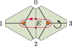
We recall the class defined before Proposition 4.39. This class depends on an orientation of , and reversing the orientation sends ; the assertions in the rest of this section hold independent of the choice of orientation.
Proposition 6.10.
The holonomy is the -sign of as defined in Definition 6.9.
Proof.
Over each domain , the fiber over the sheet labeled by vertex of is . Thus is the trivial -bundle on each connected component of . The gluing across preimages of walls is as follows. Each wall runs into a vertex . On the sheet labeled by the vertex , is glued to . The other sheet is labeled by a vertex on one side and on the other. There the gluing takes to , where
| (6.11) |
Construction 6.12.
Consider two edge-orientations , which differ by reversing the orientation on a single edge . The difference -bundle
| (6.13) |
admits a lift to a -bundle (canonical up to isomorphism)
| (6.14) |
which extends over .
For any class
| (6.15) |
Proof.
We first describe the difference bundle (6.13), as we did in the proof of Proposition 6.10. It is the trivial -bundle on each connected component of . The gluing across preimages of walls is as follows. Consider a wall ending on a vertex . On the sheet labeled by , the gluing is given by the identity element in . On the other sheet, the gluing is given by the nontrivial element in if is a vertex of , and otherwise by the identity.
Now we can define the lift : it is the trivial -bundle on each connected component of , with gluing across preimages of walls as follows. Consider a wall ending on a vertex . On the sheet labeled by , the gluing is given by . On the other sheet, if is a vertex of , then the gluing in the direction away from is given by ; if is not a vertex of , then the gluing is given by .
The holonomy of around a loop in encircling a branch point comes to , so extends across the branch points, and thus over as desired. Finally, the formula is obtained directly by evaluating both sides on arcs crossing the quadrilateral . ∎
6.3. Twistings over a triangulated surface
Now let be a triangulated surface, with edge-orientations, spin structure, and stratified abelianization data . Then define the -bundle
| (6.16) |
has trivial monodromy around each point of , and thus extends to , unlike . We use the name also for the extension.
The spin structure on is non-bounding on a circle around a branch point and thus does not extend from to , but its twist
| (6.17) |
does extend to a spin structure over .
It will be useful below to have some concrete information about this spin structure. We recall a convenient bit of notation first. Given a spin structure on a surface, and a simple closed curve , we define
| (6.18) |
We also recall the class defined before Proposition 4.39.
Proposition 6.19.
is the -sign of as defined in Definition 6.9.
Proof.
Since can be represented by the boundary of a disc in , . Thus is the monodromy of the -bundle around , which we computed in Proposition 6.10. ∎
6.4. Stratified abelianization
Fix a manifold of dimension with corners, with . Suppose is equipped with a spin structure , a spectral network , and stratified abelianization data over . Also suppose given a -bundle whose mod 2 reduction is the double cover . Then let denote the mod 4 reduction of . is a -bundle.
Theorem 6.20.
There is a canonical isomorphism
| (6.21) |
We remark that the isomorphism (6.23) is based on a choice of trivialization in Corollary 5.107. We constrain that choice in Appendix C.
Proof.
We combine ingredients as follows. First, Theorem 5.59 (triviality of Chern-Simons in unipotent directions) gives
| (6.22) |
Second, Corollary 5.107 (identity between Chern-Simons for -bundles over and -bundles over ) gives
| (6.23) |
Finally, Corollary 5.101 (invariance of spin Chern-Simons under -twists) gives
| (6.24) |
The composition of these three is the desired isomorphism. ∎
The concrete nature of the isomorphism in Theorem 6.20 depends on the nature of . In general, is an isomorphism between objects in appropriate diagram categories. For instance, if is a closed 2-manifold, is an isomorphism of lines; if is a 3-manifold with boundary, is an isomorphism of lines together with an isomorphism of objects in those lines; if is a closed 3-manifold, is just an equation.
In what follows we will need to know that has good gluing properties. These properties are most succinctly summarized as follows: they are just as if came from an isomorphism of 3-dimensional topological field theories, defined on a bordism category of oriented manifolds equipped with a spectral network, stratified abelianization data, and a lift of the double cover to a -bundle. We will apply this below to various individual manifolds carrying this data. Of the three ingredients above, two of them were formulated as isomorphisms of topological field theories; the third, Theorem 5.59, was not formulated in this language, but it was constructed in a fully local and canonical way. This is sufficient to imply the desired gluing properties.
6.5. The difference line for a triangle
Let be an oriented triangle with edge-orientations, spin structure, and stratified abelianization data

Using Chern-Simons theory on gives an object in the -line associated to the boundary ,
| (6.25) |
Using Chern-Simons theory on likewise gives an object in the -line associated to ,
| (6.26) |
Because , we cannot use Theorem 6.20 to identify these two objects. However, does not intersect , so Theorem 6.20 gives an equivalence of -lines,
| (6.27) |
Now we can compare the two objects: we define a line
| (6.28) |
We explain in Appendix C how to make a choice of isomorphism in (6.21) so that the super line is even; without further argument it could be odd.
The line depends only on , in the following sense.
Proposition 6.29.
Suppose and are triangles with edge-orientations, spin structure, and stratified abelianization data. An orientation-preserving affine-linear isomorphism which carries to induces a canonical map
| (6.30) |
An orientation-reversing affine-linear isomorphism which carries to induces a canonical map
| (6.31) |
Proof.
By uniqueness of spin structures on , we can lift to an isomorphism . By Proposition 4.33 we can lift to an isomorphism . Finally, since we can lift to an isomorphism . All of our constructions are canonical and depend only on these data, so we obtain a map as desired. It only remains to check that this map is independent of the choices we made in lifting . To see this, we need to show that the nontrivial automorphism of the spin structure—the spin flip—and the automorphism of induced by the action of and both act trivially on .
The argument that the spin flip acts trivially is the subject of Appendix C.
To show that the automorphism of acts trivially we argue as follows. Our definition of can equally well be made using rather than . In this case the whole center acts on and thus on . Now, to compute the action of the element on we consider the mapping torus , with abelianization data obtained by gluing to itself with the action of . The action of is given by the ratio
| (6.32) |
Now we consider the dependence on . Since is a flat -connection for each , and the curvature of vanishes when evaluated on a -parameter family of flat connections, it follows that gives a covariantly constant section of the bundle over with fiber . Likewise is covariantly constant. Finally, the isomorphism is flat, i.e. it is an isomorphism of line bundles with connection. Thus the ratio (6.32) is locally constant as a function of . But at it gives the action of , which is trivial; thus it must be for all , as desired. ∎
Corollary 6.33.
The line depends only on up to canonical isomorphism.
Proof.
Given and two different data and we apply Proposition 6.29 taking to be the identity map. This gives the desired isomorphism . ∎
With this corollary in mind we just write the line as . The most important feature of this line for concrete computations is that it transforms nontrivially under the rotational symmetry of , as measured by the following proposition.
Proposition 6.34.
Suppose induces a consistent orientation of , and is a positively oriented rotation by with respect to the orientation of . Then acts on as multiplication by .
Proof.
Fix stratified abelianization data and a spin structure over . Lift the action of to and , in such a way that . (This is possible, since each of and is unique up to isomorphism and has only a single nontrivial automorphism ; an arbitrary lift of will have either or , and in the latter case we replace the lift by .) Also lift to the -bundle , again in such a way that . Combining this lift with the actions of on and gives actions of on and .
We consider the -lines associated to the boundary, and . gives actions of on both -lines, the equivalence is -equivariant, and and are -invariant objects. The line
| (6.35) |
is thus acted on by , and we want to compute this action.
We will use an explicit picture of the -equivariant equivalence , obtained by chopping into three segments, ending at the midpoints of the three edges. First, we fix an -invariant trivialization of the restriction of to the midpoints. (There is a -torsor worth of freedom in this choice, which we will fix below.) Given this trivialization, we may factorize each of our -lines as a tensor product of three -lines associated to the three segments, and factorize the equivalence into a tensor product of three equivalences: for each segment , we have
| (6.36) |
Now comes the crucial technical step: for the purposes of our computation we may replace the equivalences by any other equivalences between the same -lines, compatible with the -action. Indeed, any two equivalences differ by tensorization with a line , and the -equivariance identifies the three lines with a single line , so the effect of changing from to would be to replace by ; the -action on induced by cyclic permutation of the factors is trivial, so the -action we want to compute is insensitive to this replacement.
We construct a convenient as follows. We extend the trivializations of and from the midpoints to sections and of and respectively, in an -invariant way. On each segment this gives trivializations of our two -lines, and we choose to intertwine these trivializations. Tensoring the we get
| (6.37) |
We may choose the trivialization of at the midpoints in such a way that the parallel transport of along any of the preimages of segments is given by . (Indeed, for an arbitrary -invariant trivialization, the parallel transport of along each segment is given by some fixed element ; changing the trivialization by at each vertex conjugates this transport by , and by so doing we can set the off-diagonal entries to as needed.) From now on we fix such a choice. Having done so, we can choose to be covariantly constant.
However, we cannot choose to be covariantly constant. Indeed, the parallel transport of along an edge is given, relative to the trivializations at the midpoints, by an element , where and ; in particular, . The -invariance implies that is independent of the choice of edge. Moreover, , since the holonomy of around is trivial. We choose as follows. Let be a covariantly constant section of (necessarily not -invariant). Then choose , where obeys
| (6.38) |
Now, to compute the action of on we consider the mapping torus of ,
| (6.39) |
and the mapping torus of the lift of to . The -equivariant flat bundles and induce flat bundles and respectively. Moreover, the -equivariant equivalence of -lines induces an isomorphism of lines, . The -action on is multiplication by
| (6.40) |
To compute this, first note that, being -invariant, and induce sections and of and respectively. The resulting trivializations of the boundary lines have, essentially by definition of ,
| (6.41) |
Our task now is to compute the numerator and denominator relative to these trivializations.
To compute we note that is covariantly constant on , and it can be extended to a covariantly constant section over the full ; thus the Chern-Simons form vanishes, and .
To compute is more interesting. We choose an arbitrary extension of to the solid torus . Let denote the connection form in relative to the section ; then using (3.9)
| (6.42) |
To compute explicitly, we pull back to a triple cover ,
| (6.43) |
The covariantly constant section of induces a covariantly constant section of ,303030Since is not -invariant, it would not induce a section of ; this is the reason why we had to pull back to the triple cover. which we can further extend to a covariantly constant section of . Then for some , and the invariance of under the deck group gives
| (6.44) |
The connection form in relative to is , and this form is pulled back from ; thus the integral over in (6.42) can be rewritten as one-third of a more explicit integral over ,
| (6.45) |
Moreover, is covariantly constant along translation in the -direction holding fixed, while is covariantly constant in every direction. Thus is constant in the -direction. Attaching a solid torus to along this direction we obtain a closed 3-manifold . The map naturally extends to the added , by choosing it to be constant along the factor. Then there, and thus we can replace the domain of integration in (6.45) by . This integral gives , where is the degree of the map (by which we mean the degree of the retraction of from to , when we equip with the orientation for which is a positive 3-form.) To compute this degree, we will use only the fact that commutes with certain -actions on and , as follows.
First, we can identify with as follows. On the torus , we fix coordinates , where parameterizes (positively with respect to the boundary orientation), and . These coordinates naturally extend to the two solid tori and , identifying them respectively as the loci and in . The orientation of matches the standard orientation of . The -action on becomes in these coordinates (and thus extends to a fixed-point-free action on the whole ).
Next, parameterize by . This gives . Computing in this parameterization we see that it is positive for the standard orientation on . By composing with an inner automorphism of we may assume . The -action then acts by .
Lemma 6.46.
Any continuous map commuting with the standard -action has degree equal to mod .
Proof.
Such a descends to a map which lifts to the -bundle ; this bundle has a nonzero characteristic class lying in (because the inclusion induces an isomorphism on ), and thus must act trivially on , i.e. the degree of is 1 mod 3. Since the degree of agrees with that of , this finishes the proof. ∎
To finish this section we remark on a diagrammatic perspective on which will be useful in some of the arguments to follow. Here we suppress most of the background fields to reduce clutter. We regard as a morphism in the bordism category
| (6.47) |
Applying and to this diagram, and including the map , we get
| (6.48) |
Here, and in various diagrammatic arguments to follow, we freely identify morphisms with objects of . Then the composition
| (6.49) |
6.6. Abelianization of Chern-Simons over triangulated surfaces
Now suppose given an oriented surface with a semi-ideal triangulation , edge-orientations , and a spin structure . Also fix boundary-reduced stratified abelianization data over . As we have discussed in §5.3.2, because is boundary-reduced, the -line is canonically trivial, and thus is a line. The -line is also canonically trivial, since has trivial holonomy around the boundary components; thus is also a line.
Define the difference line
| (6.50) |
Construction 6.51.
There is a canonical isomorphism of lines
| (6.52) |
Proof.
First for simplicity suppose that there are no ideal vertices, so is a closed triangulated surface.
For each we consider the dilation which rescales distance from the barycenter by . Then we have a decomposition , where is the union of the rescaled triangles .
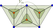
Let . To condense the notation we will just write the manifolds, suppressing all the extra background fields, including the dependence on (since is held fixed throughout this proof). Then we have a diagram in the bordism category,
| (6.53) |
Applying and to this diagram, and inserting the maps and provided by Theorem 6.20, we get the diagram below:
| (6.54) |
Now whiskering by we get a 2-morphism
| (6.55) |
Finally, defining
| (6.56) |
we have , so we can rewrite the diagram as
| (6.57) |
Composition of maps is tensor product, so this is a map of lines
| (6.58) |
as desired; what remains is to identify with the we defined in (6.50). This follows directly from (6.49) and the decomposition of into the disjoint union of triangles.
So far we discussed only the case where there are no ideal vertices. In the general case one has to draw slightly more complicated diagrams:
| (6.59) |
| (6.60) |
However, because is assumed boundary-reduced, we have trivializations of and , which are intertwined by ; using these trivializations the diagram (6.60) reduces to (6.57), and then we can proceed just as above. This completes the proof. ∎
We may also consider a family of boundary-reduced stratified abelianization data over a fixed , varying with a parameter . All of our constructions can be applied to such a family: then we obtain two invariants and both of which vary over , and an isomorphism relating them. In particular, if is a semi-ideally triangulated surface as above, then both and are line bundles over with connection, and is an isomorphism of line bundles with connection.
6.7. Reversing an edge orientation on a triangle
Now suppose is an oriented triangle with edge-orientations, spin structure, and boundary-reduced stratified abelianization data. We first consider the restriction of all the data to a single oriented edge . Let be the given orientation of and the opposite orientation. Then in the bordism category we have the diagram
| (6.61) |
Once again we suppress some background fields in the notation: we just keep the manifolds and (where necessary) the edge-orientations. We will also use freely the fact that the -bundles and are canonically trivial over .
Then we have a diagram in the 2--line :
We define
| (6.62) |
which is an automorphism of the object , or equivalently a line.
Now suppose is an oriented triangle with edge-orientations, spin structure, and stratified abelianization data. Also suppose is an edge such that agrees with the boundary orientation, and is obtained from by reversing the orientation on . Let , so now we have
| (6.63) |
Then provides an isomorphism of 2-morphisms
| (6.64) |
while gives a similar isomorphism of diagrams, but without the inner arrow,
| (6.65) |
and gives the same isomorphism of diagrams with replaced by . Combining these, we can whisker the isomorphism (6.64) into an isomorphism between the lines we previously defined in (6.49), (6.62),
| (6.66) |
This map describes the effect of reversing the orientation on one edge of .
Now we want to consider reversing orientation on two edges of . We introduce a bit of notation that will be convenient below:
Definition 6.67.
If and are edges of an oriented triangle ,
| (6.68) |
Suppose , both agree with the boundary orientation, let be obtained from by reversing , and let be obtained from by reversing both and .

We want to compare the two 2-morphisms appearing in the diagram:
Lemma 6.69.
In this situation,
| (6.70) |
Proof.
We use (5.103). For this purpose we choose a section of and maps representing , , with constant on except for . Then we have another section of , and in terms of these sections
| (6.71) |
so that the desired ratio is
| (6.72) |
∎
Proposition 6.73.
In this situation,
| (6.74) |
Proof.
Similarly we can consider reversing the orientation on an edge where the initial orientation is opposite to the boundary orientation. Then the same constructions as above give an isomorphism
| (6.76) |
6.8. Reversing an edge orientation on a triangulated surface
Now suppose is a semi-ideally triangulated surface, with boundary-reduced stratified abelianization data . Suppose , are edge-orientations on , differing by reversing the orientation on one edge . We would like to compare the maps and from Construction 6.51. Their ratio is an isomorphism
| (6.77) |
We already have an isomorphism
| (6.78) |
given by Corollary 5.101. Thus we can write
| (6.79) |
for some
| (6.80) |
This map is determined in terms of the edge-reversal maps for the two triangles , abutting , as follows.
Proposition 6.81.
.
Proof.
We decompose as indicated in the figure:
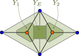
| (6.82) |
Now we want to describe relative to this decomposition. We will content ourselves with a heuristic description, leaving the full diagrammatics to the reader. On all the background fields associated to and are canonically isomorphic, and the background field is canonically trivial, so likewise is trivial. On , is described by the map where is the edge of corresponding to . Finally, on , gives the isomorphism induced by identifying these two edges. Combining these gives the desired result. ∎
Proposition 6.83.
The composition
| (6.84) |
acts by multiplication by the -sign of the edge , as defined in Definition 6.9.
7. Gluing description of the Chern-Simons line
We continue with the setup of the last section. There we used abelianization to produce an isomorphism
| (7.1) |
depending on various choices encapsulated in . In this section we process this further to turn it into an explicit description of . The final result is Theorem 7.81, which asserts the existence of nonzero elements depending on choices (including an ideal triangulation, edge-orientations, and certain choices of logarithms), and gives the cocycle expressing how changes when the data are changed.
7.1. Abelianization of Chern-Simons over interpolating 3-manifolds
Suppose is a spin 3-manifold with boundary, equipped with a spectral network such that , the restriction of to is the spectral network for a triangulation of , and has no closed components.
Each component of is a closed interval, whose two ends lie on , in two triangles , with edge-orientations , . Moreover, a tubular neighborhood of can be identified with , for a triangle with its standard spectral network. This in particular gives an orientation-reversing identification .
Now suppose given edge-orientations over , and a -bundle , which restricts to over the boundary, and also restricts to over the tubular neighborhood of each component , for some edge-orientations on . In particular restricts to match at the two ends, and so . Thus using Proposition 6.29 we get an isomorphism , i.e. an element . Tensoring over all components gives a canonical element . This element should be thought of as just implementing the matching-up of triangles provided by .
Finally, suppose we have stratified abelianization data over .
Proposition 7.2.
In this situation,
| (7.3) |
Proof.
Decompose , where is a small tubular neighborhood of . is a 3-manifold with 1-dimensional corners ; is a union of circles, which divides into a union of cylinders and a union of discs . Likewise is divided by into and .
Now we need to apply and to the various parts of this decomposition. To lighten the notation a bit we write the -lines (dimension 1)
| (7.4) |
with objects (dimension 2)
| (7.5) |
Thus , , and likewise we have , , and , . Finally, we have the elements (dimension 3)
| (7.6) | ||||
| (7.7) | ||||
| (7.8) | ||||
| (7.9) |
We can use Theorem 6.20 to construct various canonical abelianization maps: an equivalence of -lines (associated to dimension 1),
| (7.10) |
homs (associated to dimension 2),
| (7.11) | ||||
| (7.12) | ||||
| (7.13) |
and an equation (associated to dimension 3),
| (7.14) |
where
| (7.15) |
is the canonical map. Now, we define an element by
| (7.16) |
This is a measurement of the difference between the and theories on the cylinders , analogous to our definition of , but one dimension up, so it gives an element rather than a line. Tensoring (7.14) and (7.16) gives
| (7.17) |
so what remains to prove (7.3) is to show that . Each component of is a cylinder, with ends on two discs carrying the standard spectral network for a triangle; call these discs , . By a diffeomorphism we can identify this cylinder with the mapping cylinder of a map . Moreover, lifts to the spectral networks, spin structures and stratified abelianization data. Thus we can transport the computation of to the union of mapping cylinders; on each mapping cylinder this gives the action of , and then tensoring over the cylinders gives as desired. ∎
In Proposition 7.2 we only considered the case of a 3-manifold with boundary a closed triangulated surface . In applications we sometimes want to use with boundary and a semi-ideal or ideal triangulation. In this case will have to have extra boundary components extending , and corners around the ideal vertices. As long as we always work with boundary-reduced stratified abelianization data over , these extra boundary components and corners do not introduce additional complications in the formal structure: the statement and its proof are unchanged except for a bit more notation, which we omit here.
7.2. The dilogarithm in abelianization on one tetrahedron
Suppose , identified as the boundary of a tetrahedron , with the induced triangulation . Let denote a spin structure on , and stratified abelianization data over . Then extends to (uniquely up to isomorphism) and applying gives an element
| (7.18) |
Fix edge-orientations on . The goal of this section is to describe the image in terms of a relative of the dilogarithm function.
Choose a pair of opposite edges in ; as discussed above Proposition 4.39, this determines classes . Also choose a section of the -bundle and let
| (7.19) |
where denotes the connection form in the -bundle . Thus is a logarithm of . Changing the choice of section shifts each by an integer multiple of . Also let
| (7.20) |
Equivalently, is the -sign of the edge . Thus measure the isomorphism class of the spin structure on the torus , and are determined by (but have less information than) the six edge-orientations .
Proposition 7.21.
We have the relation
| (7.22) |
Proof.
Now let ,
| (7.23) |
and let
| (7.24) |
be any function obeying
| (7.25) |
Each is a variant of the dilogarithm function; see (7.69)-(7.72) for concrete examples.
Proposition 7.26.
| (7.27) |
for some independent of , .
Proof.
We first note that fits into a family of stratified abelianization data over , parameterized by , with the property . To construct this family we can use Construction 4.30, choosing the trivial flat bundle , and taking the 4 elements at the 4 vertices to have cross-ratio ; then the calculation in Remark 4.47 shows that the holonomies of will be as desired. To show that our given is indeed isomorphic to a member of this family, we use the fact that stratified abelianization data is determined up to isomorphism by the holonomies of (for this calculation see e.g. [HN]).
Because is trivial and its extension is unique, the elements sweep out a covariantly constant section of the line bundle with fibers over . Using the compatibility of with the connection in this bundle, it follows that is a covariantly constant section of the line bundle with fibers over . Moreover the section of the given deforms to a section of , unique up to homotopy. The computations in Section 4 of [FN] then show that the function
| (7.28) |
on obeys313131In [FN] we discussed only the case , but this computation is independent of . Also, beware that in this paper is in [FN], which leads to a sign flip in comparing.
| (7.29) |
This proves (7.27). ∎
7.3. Flipping an edge
Suppose given a boundary-reduced flat -bundle . Suppose , are two semi-ideal triangulations of , which differ by flipping an edge to an edge . Also suppose given a choice of sections of over the interior vertices of , such that the genericity Assumption 4.31 holds for both and . Then by Construction 4.30 we obtain boundary-reduced stratified abelianization data and over and respectively.
Let , be systems of edge-orientations on and , which agree on all common edges, i.e. all edges except for and . We would like to compare and . Their ratio is an isomorphism
| (7.30) |
To describe this map we consider the 3-manifold
| (7.31) |
Let denote the projection, and let . On we construct a SN-stratification, spectral network and stratified abelianization, as follows.
Let be the union of all the triangles in except for the two abutting . Then we have a decomposition . The stratified abelianizations and are canonically isomorphic, and thus extend to boundary-reduced stratified abelianization data over . Over we also have a -bundle .
Next we consider . Collapsing the vertical intervals in gives a surjective map , where is a tetrahedron, and this map extends to
| (7.32) |
which is a homeomorphism on the interior. On we have a standard SN-stratification and spectral network as described in Construction 4.36; pulling this back by gives a SN-stratification and spectral network on , which glue to the ones we already have on . Using Construction 4.53 we obtain stratified abelianization data over , which likewise pulls back to and glues to the stratified abelianization data we already have on .
Thus altogether we have:
-
•
A SN-stratification and spectral network over , with isomorphisms , ,
-
•
Stratified abelianization data over , which restricts to , over , respectively.
-
•
A -bundle , which restricts to , over , .
We need to extend our -twisted objects from and to : define , and twist to and to .
The stratum consists of a single point , the barycenter of the tetrahedron . Let be a small ball around . By radial projection centered at , the sphere acquires a triangulation , whose four faces correspond naturally to the two faces of and two of . comes with edge-orientations , induced by and (using the fact that and agree on the common edges). Moreover, the restriction is the spectral network , and is the restriction of to .
Now we can describe the effect of a flip on the abelianization maps :
Proposition 7.33.
The map
| (7.34) |
is the product
| (7.35) |
Proof.
We apply Proposition 7.2 to the 3-manifold , noting that what was called there is here the disconnected boundary , which carries a semi-ideal triangulation and edge-orientations .
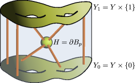
This gives the formula
| (7.36) |
Tensoring with then gives
| (7.37) |
But since and , is the identity map on ; the desired result follows by rearranging factors. ∎
7.4. Gluing the Chern-Simons line
Let be a compact oriented surface with boundary. Suppose is a flat boundary-reduced -bundle. In this section we use abelianization to give a description of the line .
Construction 7.39.
We consider tuples , where:
-
•
is a semi-ideal triangulation of ,
-
•
is a system of edge-orientations for ,
-
•
is a flat section of over each , such that if is an ideal vertex then the projection of to agrees with the boundary reduction,
-
•
is a collection of complex numbers, where
(7.40) if is an edge with vertices . Here means the continuation of from by parallel transport along the edge , similarly , and the wedge product is evaluated at any point along ; here and below, we use the fact that is an -bundle and thus there is a canonical volume form in .
For each such tuple there is a canonical isomorphism
| (7.41) |
Proof.
Fix and as above. Construction 4.30 extends to stratified abelianization data over . Then Construction 6.51 gives an isomorphism
| (7.42) |
Using the data we determine a section of the line bundle (up to homotopy), as follows. Recall that each has two preimages and in . Each determines an element of the fiber of . We also determine an element by the condition . Now suppose with vertices , . The parallel transport of along preimages of takes
| (7.43) |
The choice of a logarithm thus determines (up to homotopy) an extension of over the preimages of . Finally, by construction has zero winding around the preimage of the boundary of each triangle, because the summands and cancel over each of the three edges; thus can be extended to a section of , uniquely up to homotopy. The section determines a trivialization . Then we define
| (7.44) |
∎
We remark that the existence of the data above requires , i.e. that the genericity Assumption 4.31 is satisfied.
Proposition 7.45.
We have relations among the maps associated to data and as follows:
-
(1)
Suppose and differ only by a change involving a single vertex : and for all edges incident on . Then
(7.46) -
(2)
Suppose and differ only by a change involving a single edge : and .
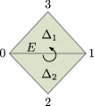
Figure 23. The quadrilateral . -
(3)
Suppose and differ only in that is obtained from by flipping edge to obtain a new edge , with some orientation and a choice of logarithm .
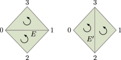
Figure 24. The quadrilaterals in and in , related by a flip.
Proof.
We treat the three relations in turn:
-
(1)
In this case the sections and are homotopic (the homotopy obtained by continuously varying from to ) and thus they induce the same trivialization of .
-
(2)
By (7.44) and (6.79) we have . We use Proposition 6.81 to expand the factor. For the factor, we use (5.103), which gives
(7.52) where denotes the connection form on . By (6.15) the multiplicative factor here is
(7.53) and comparing (7.47) to the definition of , we have , so the factor becomes
(7.54) as desired.
-
(3)
We use the setup and notation of §7.3, involving the 3-manifold . Proposition 7.33 gives as a tensor product of three ingredients:
-
(a)
First we have . The data of and in particular determine sections and of on the boundaries and , as discussed in Construction 7.39. There is a section of which extends and ; let be its restriction to . The Chern-Simons form vanishes for a flat bundle; it follows that
(7.55) - (b)
-
(c)
Finally we have the isomorphism .
Tensoring these ingredients together, and using the definition (7.44) of and the definition (7.38) of , we get the desired (7.51).
-
(a)
∎
7.5. Explicit formulas
In the last section we gave a description of the line which is canonical but somewhat inexplicit: the transition maps described by Proposition 7.45 involve the maps and , for which we have not yet written down concrete formulas. Roughly speaking, we have fully described the -dependence in , but left some constant phases undetermined. In this section we rectify this omission, getting concrete formulas in terms of actual numbers, at the cost of making some arbitrary choices.
7.5.1. Trivializing the difference lines
Let denote the standard triangle with its standard orientation, and vertices labeled 012 in cyclic order given by the orientation.
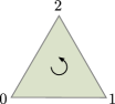
We choose a nonzero element
| (7.56) |
for each of the eight possible . We may choose so that if is a rotation which acts on the vertices by ,323232The factor appearing in (7.57) is dictated by Proposition 6.34.
| (7.57) |
and also if is the reflection which acts on the vertices by ,
| (7.58) |
From now on we assume that we make such a choice.
Now suppose is a general triangulated manifold with edge-orientations. We want to trivialize the line ; for this we need one more datum:
-
•
A marked edge on each .
The edge determines an orientation-preserving identification , by the condition that takes the edge to . Then, given the extended data we obtain a trivialization
| (7.59) |
What remains is to describe the relations between the elements associated to different .
7.5.2. Computing
Recall the edge-reversal map from §6.7. Fix arbitrarily a nonzero element in the line considered there, and then define constants by
| (7.60) |
Our aim now is to compute these constants. We write each as a 3-tuple .
Proposition 7.61.
We have
| (7.62) |
and for some we have
where .
Proof.
Next, using Proposition 6.83, we have
| (7.65) |
Finally, using the reflection condition (7.58) gives
| (7.66) |
which implies in particular
| (7.67) |
and
| (7.68) |
Proposition 7.61 determines all of the in terms of the undetermined constants , . Fixing , is equivalent to fixing the remaining freedom in the trivializations , up to an overall scale which remains unfixed.
7.5.3. Fixing the
In §7.2 we determined the functions up to an overall constant. We now make a definite choice as follows. Let denote the principal branch of the dilogarithm function, which has a branch cut along . Then let
| (7.69) | ||||
| (7.70) | ||||
| (7.71) | ||||
| (7.72) |
It is routine to check that these formulas indeed define holomorphic functions : the discontinuity of across its branch cut gets compensated by the discontinuity of the floor function, up to an integer multiple of . Using the differential equation obeyed by , it is also straightforward to check that they obey (7.25) as needed.
7.5.4. Computing the
Now that we have fixed our choices of and also fixed trivializations of the we are in position to express the normalization constants from (7.38),
| (7.73) |
as concrete numbers: we write
| (7.74) |
for some .
To compute the , it will be useful to recall their origin in Chern-Simons theory on an oriented sphere with tetrahedral triangulation , obtained by gluing to along the common boundary. We label the edges of and as shown in Figure 24, thus identifying with a standard model. We use to represent the full collection of six edge-orientations on induced by , and use the condensed notation for .
The next lemma concerns just , not the original surface .
Lemma 7.75.
Suppose and are two systems of edge-orientations on , which differ by reversing the orientation on some . Fix stratified abelianization data on , and extend to data as in Construction 7.39. Also define where , and for all other edges. Let and be given by (7.49) and (7.50), likewise and . Let , denote the two triangles abutting . Then
| (7.76) |
with determined in Proposition 7.61.
Proof.
We consider the element , which has
| (7.77) |
Part (2) of Proposition 7.45 gives the relation between and . The quantity appearing there is not necessarily the here, because is not necessarily ; one can show however (e.g. by checking the six cases for ) that the correct relation is
| (7.78) |
Thus we get
| (7.79) |
Now for each let the marked edge be either or , whichever lies on . Dividing both sides by gives the desired result. ∎
Lemma 7.75 determines the constants up to a single overall multiplicative constant. The remaining constant can be fixed as follows. We consider a triangulated surface with stratified abelianization data . Suppose contains three triangles which make up a pentagon. Then we consider two possible sequences of flips, involving various triangulations as indicated in Figure 26, and choose data (logarithms, edge-orientations and marked edges) extending the triangulations .
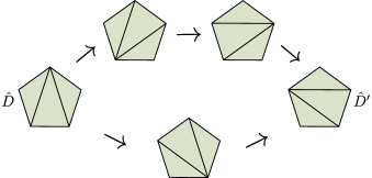
Since both sequences begin at and end at , we can follow either sequence to compute the ratio ; but one sequence contains flips and the other contains , so requiring that they are equal is enough to determine the overall multiplicative constant in . Carrying this computation out we obtain the following (the detailed computation can be found in the file dilog-compute.nb included with the arXiv version of this paper.)
Lemma 7.80.
If we set , then , with given below. We specify by the tuple .
7.5.5. The final result
We summarize our description of the Chern-Simons line, in its most concrete form:
Theorem 7.81.
Fix a surface and a boundary-reduced flat -bundle . We consider tuples , where:
-
•
is a semi-ideal triangulation of ,
-
•
is a system of edge-orientations for ,
-
•
is a flat section of over each , which when projected to agrees with the boundary reduction,
-
•
is a collection of complex numbers, where if is an edge with vertices ,
-
•
is a system of marked edges, where is an edge of .
For each such tuple there is a canonical nonzero element
| (7.82) |
They obey relations as follows.
-
(1)
Suppose and differ only by a change involving a single vertex : and for all edges incident on . Then
(7.83) -
(2)
Suppose and differ only by changing the marking to for a single triangle . Then
(7.84) - (3)
-
(4)
Suppose and differ only in that is obtained from by flipping edge to obtain a new edge , with some orientation and a choice of logarithm . Suppose that the triangles abutting in both have , and the triangles abutting in both have . Labeling the edges of and as in Figure 24, define , , , by (7.49), (7.50). Then
(7.86)
Proof.
Theorem 7.81 closely resembles known patching constructions of a prequantum line bundle over a symplectic leaf of the -character variety of a punctured surface. In particular, in [FG2] such a line bundle is constructed in the more general setting of an -cluster variety, using the dilogarithm as a gluing map. Related constructions appear in the subsequent works [N, APP, BK, CLT].333333In all of these works the basic dilogarithmic formula for transition functions appears, but the detailed treatment of the constant factors is somewhat different in each case. In all these cases, the characteristic property of is that it carries a natural connection given concretely in terms of the cluster coordinates on the character variety. From our point of view, this connection is the one provided by the TFT applied to families of flat -bundles , the cluster coordinates are (up to sign) the holonomies of the corresponding flat -bundles , and the fact that the connection has a simple expression in cluster coordinates is obtained by using to pass from to .
8. Computing CS invariants for flat -bundles over 3-manifolds
Let be an oriented -manifold with boundary. Suppose is a boundary-reduced flat -bundle. In this section we explain how to use our results to obtain a dilogarithmic formula for the Chern-Simons invariant , Theorem 8.8 below, assuming that satisfies a genericity condition. This formula closely resembles the previously known formulas we recalled in §2, but its precise structure is slightly different, involving several variants of the dilogarithm function and some extra cube roots of unity, and not requiring any orderability constraints on the triangulation of .
8.1. Abelianization of the CS invariant
We fix data:
-
•
a semi-ideal triangulation of , such that the genericity Assumption 4.31 is satisfied.
-
•
a system of edge-orientations for .
According to Construction 4.53, determines a spectral network on , and extends to boundary-reduced stratified abelianization data over .
The edge-orientations determine a lift of the double cover to a -bundle over each face of by Construction 6.5. We can then extend by radial projection to get a -bundle . As before, we use this to twist to , and to , both of which extend over .
For each tetrahedron we introduce a small ball around the barycenter, and define . As we discussed in §7.3, is naturally triangulated and has edge-orientations induced from those of . Then we have
| (8.1) |
Moreover, each is pierced by a component of the branch locus which connects a triangle in to another triangle in , and thus gives an element
| (8.2) |
Tensoring over all faces gives an element
| (8.3) |
Proposition 8.4.
The Chern-Simons invariant is
| (8.5) |
Proof.
Apply Proposition 7.2 to the 3-manifold . This gives
| (8.6) |
Then gluing in a factor for each gives the desired formula. ∎
8.2. Explicit formulas
To make the formula in Proposition 8.4 more concrete, we fix more data:
-
•
a flat section of over each , lying in the line given by the boundary reduction if is an ideal vertex,
-
•
a collection of complex numbers, where if is an edge with vertices .
-
•
a pair of opposite edges on each tetrahedron.
Note that induces a marked edge for each face of . Each face has two abutting tetrahedra , , and the marked edges coming from these two tetrahedra need not agree. Suppose we equip with the boundary orientation induced by ; then we can consider the pairing which measures the mismatch. Note that this quantity is independent of which tetrahedron we called , since that choice enters both in the orientation of and in the ordering of the antisymmetric pairing.
Fix a , and let denote one of the marked edges ; then let , be defined by following around a face, with . Then define
| (8.7) |
and let be the -sign of the edge . Then we have the following concrete formula for the Chern-Simons invariant:
Theorem 8.8.
Proof.
As in Construction 7.39, the choice of logarithms determines a section of over each face; using radial projection in each tetrahedron, this extends to a section of . Then, using the fact that the Chern-Simons form vanishes for a flat bundle, we have
| (8.9) |
We plug this into the formula of Proposition 8.4, which gives
| (8.10) |
On each , we have
| (8.11) |
Applying to this tensor product pairs up the factors corresponding to the same face on different tetrahedra. For a face where the marked edges and agree, this pairing just gives , using (7.58). More generally, using (7.57), we see that the pairing is . Plugging this into (8.10) gives the desired result. ∎
8.3. An example
Let be the ideally triangulated manifold obtained by gluing two copies , of the standard oriented tetrahedron across the four triangles , with each gluing specified by giving the mapping between three vertices of and three vertices of : 343434This manifold is known as the “figure-eight sister,” or m003 in the SnapPea census. To avoid confusion we note that it is not the figure-eight knot complement; the latter is also obtained by gluing two tetrahedra, but it does not admit a boundary-unipotent -connection — although it does have boundary-unipotent -connections, e.g. the one induced by the hyperbolic structure. See [C] for a general discussion of the obstruction to lifting a boundary-unipotent -connection to a boundary-unipotent -connection.
The induced orientations on each face are such that the vertex orderings shown above are positively oriented on , negatively oriented on . This gluing induces identifications on vertices and edges; after the gluing there is vertex and edges. Choose edge-orientations so that points from in and points from in . See Figure 27.
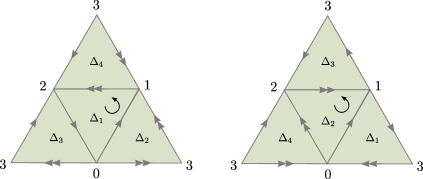
Suppose given a flat -bundle , with a section chosen at the vertex. Write if is an edge from to and . The corresponding to the edges of a single tetrahedron are constrained by the “Ptolemy relation”:353535These relations are exploited systematically in [GGZ1, GGZ2] to parameterize flat bundles over triangulated 3-manifolds. if we have four elements in a 2-dimensional vector space then
| (8.12) |
Applying this to we get the relation
| (8.13) |
As it happens, in we get the same relation.363636Had we used the figure-eight knot complement instead, we would have gotten a sign flipped here, with the result that the only common solution of the two equations would be . Assuming that , we may choose the scale of so that , and then using (8.13)
| (8.14) |
For either choice of the sign in (8.14), we can build a flat boundary-reduced -bundle , by taking the trivial bundle in each tetrahedron and then gluing across each triangle, requiring that the gluing match up the sections at the three vertices of the triangle. In this way we obtain two inequivalent flat boundary-reduced -bundles . Moreover, since all these -bundles obey the genericity Assumption 4.31.
In either case, we would like to compute using Theorem 8.8. For this we have to make a choice of a pair of marked edges on each tetrahedron. We choose the edges labeled ,. We also have to choose logarithms of . Then for either or we have
| (8.15) |
To be completely explicit let us choose corresponding to the sign in (8.14) above. Then, using (7.69) and (8.14), it turns out that373737The fact that we get a closed form expression here comes from the fact that, for , we have the closed form expression . Also, in this example is actually independent of the choice of logarithms , . Both of these are exceptional properties, which do not hold in most examples; more typically, the final result for involves a sum of for algebraic numbers , and changing the choice of logarithms changes the contributions from individual tetrahedra while leaving the final result unchanged.
| (8.16) |
Next we look up from Lemma 7.80 that for either tetrahedron we have
| (8.17) |
Finally, we have to include the cube roots of unity from face gluings. For instance, on face we see from the face gluings above that the edge (numbered on ) and the edge (numbered on ) have . Computing similarly for the other three faces, we get the overall factor
| (8.18) |
Combining the factors (8.16) (for each tetrahedron), (8.17) (for each tetrahedron), and (8.18) we get
| (8.19) |
8.4. Another example
Now let be the manifold called m071 in the SnapPea census. admits an ideal triangulation with 5 tetrahedra, 10 triangles, 5 edges and 1 vertex. Applying Theorem 8.8 in this example we obtain the Chern-Simons invariants for inequivalent boundary-reduced flat -bundles : numerically they are approximately
Details of this computation (along with a few others) are given in the Mathematica notebook dilog-compute.nb, available as an ancillary file included with the arXiv preprint version of this paper. In making these computations we made use of the software SnapPy [CDGW] and Regina [BBP].
9. Future directions
We conclude with a brief description of possible avenues for further exploration.
- 1.
- 2.
-
3.
The flat -connections to which we apply stratified abelianization are assumed to be boundary-unipotent, this for both 2- and 3-dimensional compact manifolds with boundary. The expectation is that the boundary-unipotent assumption could be dropped at the cost of having additional lines or -lines associated to boundary components.
-
4.
The 3-dimensional spectral networks in this paper are either induced from a triangulation or for the Cartesian product of a triangulated 2-manifold and a closed interval (§7.3). According to [GMN3] one obtains a 3-dimensional spectral network from a 1-parameter family of holomorphic quadratic differentials on a Riemann surface. This recovers the spectral network of §7.3, but one can also get another transition of triangulations called a “juggle”. It would be interesting to study this kind of 3-dimensional spectral network.
-
5.
One can strive to develop spectral networks (rank one or higher rank) as a topological structure on a smooth manifold, much like an orientation or spin structure. If so, then one could define bordism categories and bordism spectra as domains of field theories on manifolds equipped with a spectral network and stratified abelianization. This should lead to more powerful theorems. Perhaps, then, our main results could be stated and proved as parts of an isomorphism of field theories.
-
6.
One of the most important aspects of 2-dimensional spectral networks is the relationship to the WKB analysis of ordinary differential equations; see e.g. [KaTa, GMN3] and references therein. One can inquire whether 3-dimensional spectral networks have a similar relationship to differential equations.
-
7.
We give a construction of the Chern-Simons line of a flat bundle on a 2-manifold via stratified abelianization. In a parametrized family of flat bundles, this gives a construction of the Chern-Simons line bundle with its covariant derivative. This is the same construction that appears in [FG2, APP, N, CLT], and therefore the line bundle constructed in those papers must be the Chern-Simons line bundle. One can imagine that this identification of the line bundle will lead to new insights and results.
-
8.
2d spectral networks on a Riemann surface can be constructed in terms of BPS particles in a corresponding supersymmetric quantum field theory [GMN1]. It would be very interesting to know whether one can understand 3d spectral networks in a similar way; candidates for the corresponding quantum field theory are known in the physics literature, beginning with [DGGu].
-
9.
2d spectral networks can be used to construct the quantum trace map (or -nonabelianization map, or quantum UV-IR map) of [BW], as a homomorphism from the skein algebra of a surface to the skein algebra of a double cover [G, NY]. It would be interesting to use the 3d spectral networks defined in this paper to construct a 3-manifold version of the quantum trace, mapping the skein module of a 3-manifold to an skein module of a branched double cover . According to the recent proposal of [AGLR], such a 3-manifold quantum trace is one of the necessary ingredients in the formulation of a “length conjecture” for link invariants.
Appendix A Ordinary differential cochains
Differential cohomology descends on the one hand from the differential characters of Cheeger-Simons [ChS] and on the other from Deligne cohomology [De] in algebraic geometry. The ideas for an explicit model are suggested in [DF, §6.3]. Hopkins and Singer [HS, §3] develop the model that we recall in this appendix. The theory of generalized differential cohomology (and differential cocycles) has been further developed in many works, for example [SS, BNV, ADH]. In this brief appendix we also include a few complements needed for Chern-Simons theory.
A.1. Cochain model
Let be a smooth manifold, an abelian group, and the group of singular -cochains with values in the abelian group . For each define a cochain complex by
| (A.1) |
with differential acting on , , or on , , given by
| (A.2) | ||||
The cohomology of the cochain complex is
| (A.3) |
and the diagonal group is the differential cohomology. Since we have great use for the diagonal groups, we introduce the notations
| (A.4) | ||||
where is the subgroup of cocycles. The group is isomorphic to the group of Cheeger-Simons differential characters on . It can be given [BSS], [DGRW, §6] the structure of an infinite dimensional abelian Lie group with Lie algebra and homotopy groups
| (A.5) | ||||
Remark A.6.
-
(1)
The case is instructive: is isomorphic to the group of isomorphism classes of principal -bundles with connection over .
-
(2)
In the main text we use complex differential forms and complex singular cochains in (A.1), for which we use the notation ‘’.
- (3)
-
(4)
There are alternative models which replace singular cochains with integer coefficients by other models of cochains or by maps to Eilenberg-MacLane spaces. The latter approach is used to define differential versions of generalized cohomology theories, as in [HS, §4].
A.2. Curvature, characteristic class, and nonflat trivializations
The projection
| (A.7) |
is called the curvature or covariant derivative map, depending on the context. The restriction of (A.7) to differential cocycles factors through and has image the subgroup of closed differential forms with integral periods. There is also a characteristic class homomorphism
| (A.8) |
The short exact sequence
| (A.9) |
induces a long exact sequence in cohomology:
| (A.10) |
Let be a differential cocycle.
Definition A.11.
A cochain is a nonflat383838‘Nonflat’ could be replaced by the more accurate ‘not necessarily flat’. trivialization of if holds in .
By (A.10), a nonflat trivialization produces a differential form , the covariant derivative of . (It is the image of under (A.7).) For we can represent as a complex line bundle with connection. Then a nonflat trivialization is a section of , and its covariant derivative is as usual.
Remark A.12.
See [F3, Definition 5.12] for a model of nonflat trivializations which works in generalized differential cohomology theories.
A.3. Higher Picard groupoids of differential cocycles
As a warmup, recall that a cochain complex
| (A.13) |
gives rise to a sequence of higher Picard groupoids. For , form the truncated complex
| (A.14) |
in which is the subgroup of closed elements. Define the Picard -groupoid as follows. The set of objects is . The -torsor of 1-morphisms between is
| (A.15) |
The -torsor of 2-morphisms between is
| (A.16) |
and so on. The homotopy groups of are
| (A.17) |
A variation of this construction produces higher Picard groupoids out of differential cohomology on a smooth manifold . Define the Picard -groupoid to have as its set of objects , the set of differential cocycles of degree . Then for , define
| (A.18) |
where as in Definition A.11 the equation lies in . In other words, is a nonflat trivialization of . Now for , define
| (A.19) |
The homotopy groups of are the differential cohomology groups:
| (A.20) |
Remark A.21.
In low degrees the have alternative, more geometric, presentations. For example, is equivalent to the following Picard 2-groupoid: an object is a principal -bundle with connection ; a morphism is a section of ; and a 2-morphism is a function such that , where is the mod reduction of .
A.4. Integration and Stokes’ theorem
We repeat and expand upon material from [HS, §3.4], slightly specialized. Let be a proper fiber bundle whose base is a smooth manifold and whose total space is a smooth manifold with boundary; the fibers of are smooth manifolds with boundary. Suppose an -orientation is given; see [HS, §2.4]. Then if the fibers have dimension , integration is a homomorphism
| (A.22) |
We also have the usual integration of differential forms, and the diagram
| (A.23) |
commutes. Also the integration map (A.22) commutes with base change.
We state a version of Stokes’ theorem in this context. It concerns the case in (A.22), restricted to differential cocycles.393939We do not vouch for the signs.
Theorem A.24.
Let be a differential cocycle with curvature . Then the integral is a nonflat trivialization of with covariant derivative .
See [HS, §3.4] for a more general theorem and proof.
We also need a generalization of Theorem A.24 to manifolds with corners. Here we state the next simplest version—corners of codimension at most 2—and leave to the reader the more general version. For convenience we use manifolds with corners equipped with the extra structure needed for objects and morphisms in bordism multicategories, as in [FT1, §A.2]. The data of such a manifold of dimension and depth includes manifolds with corners of depth , , , and embeddings . The data is designed to fit the formalism of multicategories. For example, if then a 2-categorical interpretation has objects ; 1-morphisms ; and itself is a 2-morphism .
Let be a proper fiber bundle whose base is a smooth manifold and whose total space is a manifold with corners of depth . Assume that carries the extra structure of [FT1, §A.2], fibered over . In particular, there are fiber bundles , , . Let be a differential cocycle with curvature . Define
| (A.25) | ||||||
These formulas pertain for , ; for omit .
Theorem A.26.
-
(1)
is a nonflat trivialization of with covariant derivative .
-
(2)
is a nonflat trivialization of with covariant derivative .
The diagram
| (A.27) |
captures some of Theorem A.26. In the terms of §A.3, the integral of over is a 2-morphism in . We leave generalizations to greater depths to the reader.
We also use a generalization of Theorem A.26 for the integral of a 1-morphism in . For simplicity, consider a 1-morphism of the form . In other words, is a nonflat trivialization of . Let be the covariant derivative of . As in (A.25), set
| (A.28) | ||||||
Theorem A.29.
-
(1)
is a nonflat trivialization of with covariant derivative .
-
(2)
is a nonflat isomorphism with covariant derivative .
-
(3)
is a nonflat isomorphism with covariant derivative .
The data of assemble to a 3-morphism in . We depict all but in (A.30).
| (A.30) |
Again, we leave to the reader generalizations of Theorem A.29 to greater depths.
Remark A.31.
Suppose , so that (A.30) is a diagram in . Then as in Remark A.21 we interpret as a principal -bundle with connection, as a nonflat isomorphism , and as a function whose reduction mod maps the isomorphism to the isomorphism . Now is a nonflat section of . The isomorphism maps to a section of , and is a function whose mod reduction maps the section to the section . Finally, trivially—there are no nonzero 3-morphisms in —which means that the difference of the functions equals the function , as is evident from the foregoing.
Appendix B Invertible field theories
We briefly outline some general facts about invertible field theories, including those which are not flat, hence not topological. For simplicity we confine our exposition to a setting which applies to the Chern-Simons we encounter in §5.3.5. Invertible field theories which are topological in a restricted sense (which applies to evaluation on a single manifold, as for example is true for Chern-Simons theory (3.13) on flat connections) or are topological in a strong sense (which applies to evaluation in families) are modeled as maps of spectra in topology; see [FHT, FH1, F5] and the references therein. Here we use generalized differential cohomology, for which we need a model of “cocycles” which generalize the singular cocycles used in Appendix A. For background and detailed development of topics in this appendix, see [FH2, HS, BNV, ADH] and the references therein.
Let be a Lie group. Let denote the category of smooth manifolds and smooth maps between them, and let be the category of simplicial sets. Then
| (B.1) |
is the simplicial sheaf which assigns to a test manifold the nerve of the groupoid of -connections on ; see [FH2, Example 5.11]. Similarly,
| (B.2) |
is the simplicial sheaf which assigns to a test manifold the nerve of the groupoid of -connections on and a trivialization of the underlying -bundle. Then is equivalent to the set-valued sheaf which assigns to a test manifold the vector space , where is the Lie algebra of ; see [FH2, Example 5.14]. A smooth manifold defines a representable set-valued sheaf on ; its value on a test manifold is the set of smooth maps .
Let be a generalized cohomology theory. Define the -graded real vector space
| (B.3) |
and suppose given an isomorphism of cohomology theories , where the codomain is the Eilenberg-MacLane theory with . There is then a differential cohomology theory (of “Hopkins-Singer type”) which refines the topological theory . Furthermore, these theories—as well as the de Rham complex—can be evaluated on simplicial sheaves, in particular on . The Anderson dual to the sphere is a universal choice for the codomain of an invertible field theory. Nonetheless, for Chern-Simons theory in this context it is more convenient to use a truncation , the cohomology theory introduced in §5.2.1, as the codomain.
Remark B.4.
Chern-Simons theory has not only a -connection as a background field, but also a spin structure. In the formalism sketched here we do not treat them symmetrically: we use the spin structure to integrate differential -cohomology classes (and cochains). By contrast, in topological invertible theories we usually do treat them symmetrically and use the universal codomain .
An -dimensional invertible field theory on -connections is modeled by a map
| (B.5) | ||||
| The theory has an underlying cohomology class | ||||
| (B.6) | ||||
| and curvature | ||||
| (B.7) | ||||
of total degree . (For -cohomology404040In the main text we use a complexified version of differential -cohomology. the -graded vector space is supported in degree 0, hence the codomain of the curvature (B.7) is .) The theory is flat if its curvature (B.7) vanishes. In that case factors through a topological theory
| (B.8) |
where is the cofiber of . The theory is topologically trivial if its underlying cohomology class (B.6) vanishes. A trivialization of the underlying cohomology class lifts to a theory defined by the differential form414141Our convention is that the partition function for a theory defined by a form is obtained by integrating .
| (B.9) |
(Compare with Definition A.11 and the following paragraph.) Conversely, a differential form (B.9) determines an invertible theory (B.5), and the isomorphism class of the latter does not change if the form is shifted by an exact form (or, more generally, by a closed form whose periods are integral in a sense defined by the cohomology theory ).
Example B.10.
The 3-dimensional spin Chern-Simons theory in §5.3.5 is a map
| (B.11) |
Recall [FH2] that the complexified de Rham complex of is a complex polynomial algebra generated by a 2-form which is times the curvature of the universal -connection. Then the curvature of the theory (B.11) is the 4-form
| (B.12) |
The curvature, and indeed the entire theory (B.11), should be evaluated on families
| (B.13) |
in which is a proper fiber bundle equipped with a relative spin structure and is a principal -bundle equipped with a connection. Then (B.12) pulls back to an element of .
The discussions in §A.2 and §A.3 have analogs for invertible field theories. Thus there is a notion of a flat (or nonflat) isomorphism of invertible theories. Furthermore, the equivalence classes of flat isomorphisms of two -dimensional invertible theories form a torsor over the abelian group of flat -dimensional invertible theories. The latter are topological invertible theories in a strong sense, hence may be treated via methods of stable homotopy theory.
Appendix C gradings
The invertible spin Chern-Simons theory is obtained by integration in the cohomology theory with two nonzero homotopy groups; see §5.2.1. (As explained in §5.3, one integrates complex differential “cochains” in the differential theory or, for flat connections, “cochains” in the secondary theory .) The homotopy group , which appears along with the standard or , introduces an additional -grading in the values of the field theory. In this appendix we collect some remarks and results about this grading. In particular, we complete the proof of Proposition 6.29. The bottom line is: with a suitable universal choice we can and do ignore the -gradings in the main text.
C.1. -lines
Let be the linear category of complex -graded424242As usual, we use ‘super’ as a synonym for ‘-graded’. vector spaces; for the hom space consists of even linear maps . Impose the symmetric monoidal structure of tensor product with the Koszul sign rule. A super category is a complex linear module category over the tensor category . Super categories form a 2-category. The multiplicative units in this 2-category are called -lines, and there are two such up to isomorphism: the Bose line and the Fermi line ; the latter is the category of modules over the complex Clifford algebra . An automorphism of an -line is a functor defined by tensoring with a super line ; the complex line can be even or odd. We refer to [FT2] for more details about super categories.
Remark C.1.
The integral of the level of spin Chern-Simons theory over a spin 2-manifold with flat -connection lies in . The nonzero homotopy groups of are and ; there is a nonzero -invariant which connects them. An equivalent linear Picard groupoid is that of complex super lines, and so the value of on a closed 2-manifold is a complex super line. Similarly, on a spin 1-manifold the relevant space is , whose nonzero homotopy groups are and . An equivalent linear Picard 2-groupoid is that of Bose -lines. In particular, we do not encounter Fermi -lines. (We would have met Fermi -lines had the level lain in the cohomology theory with an additional homotopy group .)
C.2. Spin flip
A Riemannian spin -manifold is a Riemannian manifold equipped with a principal -bundle which lifts the orthonormal frame bundle under the homomorphism . A diffeomorphism of spin -manifolds is an isometry of the underlying Riemannian manifolds together with a lift to the -bundles. The spin flip is the automorphism with lift given as multiplication by the central element of .
Let be an -dimensional field theory of spin manifolds—say nonextended—so defined on a bordism category of - and -manifolds. If is a closed spin -manifold, then is a super vector space. We say that satisfies spin-statistics if the spin flip acts on the super vector space as the grading automorphism . Any which is topological, invertible, and reflection positive satisfies spin-statistics [FH1, §11]. Complex Chern-Simons theories are not reflection positive, and in any case what we need is spin-statistics for the difference line of a triangle, which is defined in §6.5 via a combination of the spin Chern-Simons theory , the Chern-Simons theory , and the abelianization isomorphism (6.21). Although we cannot simply quote [FH1, §11] for what we need, the basic setup pertains, and so we review it briefly.
Let be a symmetric monoidal category, and suppose is a dualizable object. Then
| (C.2) |
is by definition the dimension . For example, if and is a finite dimensional super vector space, then . If is a morphism, then the composition
| (C.3) |
is by definition the trace . For and an (even) endomorphism of , this categorical trace is usually called the supertrace. For the spin bordism category and a closed spin -manifold with spin flip , we find
| (C.4) | ||||
where ‘(non)bounding’ identifies the spin structure on . If is a topological field theory, then since is a symmetric monoidal functor it maps traces to traces:
| (C.5) |
If is invertible, then spin-statistics holds for iff this equals ; spin statistics holds for iff this equals for all .
C.3. Spin-statistics for the difference line
Next, recall the construction of the complex line , defined in (6.28) in an equivalent description to what we give here. Let be the standard spin 2-disk; the spin structure is denoted . The edge orientations which appear on the triangle in (6.28) give rise to a universal cover of ; see 6.1. The 2-disk is equipped with its standard spectral network (Figure 25), and is stratified abelianization data (Definition 4.23).
The line derives from three ingredients. First Chern-Simons theory on produces an -line434343The Chern-Simons theory does not use the spin structure and it factors through ungraded linear objects, so is canonically a -line. Here we base extend to for consistency with . and an isomorphism of -lines
| (C.6) |
Let be the center point of and let the double cover constructed from the spectral network on . The spin structure lifts to a spin structure on the deleted 2-disk ; does not extend over the deleted point. The principal -bundle derived from is used to twist this spin structure and the flat -bundle over —see §6.3—to obtain a spin structure and a flat -bundle over the filled-in 2-disk . The second ingredient in is then the -spin Chern-Simons invariant
| (C.7) |
The third ingredient is the isomorphism of -lines
| (C.8) |
constructed in §6.4. For now we simply note that is the composition of three isomorphisms; we dig into the details in §C.4 below. Finally, the line is the composition
| (C.9) |
That is, the right hand side of (C.9) is an -linear automorphism of , hence it is tensoring with a line . Note that is -graded; it may be even or odd.
Let denote the spin flip of the spin 2-disk . It induces the spin flip of , and these spin flips of 2-disks restrict to the spin flip of the boundary circles. In this way induces an involution on each of (C.6), (C.7), and (C.8), hence too an involution on the line which is their composition.
Proposition C.10.
if is even, and if is odd.
Proof.
Define an invertible 1-dimensional field theory of spin manifolds as follows. If is a compact 0-dimensional spin manifold or a 1-dimensional spin bordism, then form the spin manifold and equip it with the structure pulled back from on . Then is computed as the composition in (C.9) applied to :
| (C.11) |
Note that . By (C.5) the supertrace of is
| (C.12) |
Hence the proposition follows if we prove that satisfies spin-statistics.
Compute as the composition (C.11). Write . The complex lines and have nonzero (basis) elements and . Furthermore, since is a map of theories, the linear isomorphism
| (C.13) |
maps to . It remains to compute the ratio of each of the vectors and and these basis elements. The first ratio is evaluated on
| (C.14) |
and the second ratio is evaluated on
| (C.15) |
where the minus sign denotes the opposite spin structure (and reverse orientation). But each of these is a 3-sphere with the trivial connection, and so each partition function is . It follows that , as claimed. ∎
Remark C.16.
In the proof we encounter the 3-sphere in (C.14) with the following spectral network. The branch locus is an embedded . The walls are three disjoint embedded open 2-disks , each of which has boundary .
C.4. The freedom to eliminate odd lines
The isomorphism is the composition of three isomorphisms: see Theorem 6.20. One of them, (6.22), is given by a canonical construction in Theorem 5.59. We fixed another, (6.24), in Corollary 5.101. The remaining isomorphism in (6.23) derives from Corollary 5.107, which we did not fix completely. Namely, since is an isomorphism of invertible 3-dimensional topological theories, we can tensor it with an invertible 2-dimensional theory to obtain a new isomorphism. The background fields of —listed at the beginning of §5.3.6, are: a spin structure , a flat -connection, and a principal -bundle which lifts the associated principal -bundle . Observe that the 2-dimensional invertible theory whose partition function is444444This is the Arf invariant (0 or 1) of the shifted spin structure . takes value the odd line on . Hence, possibly after tensoring with this shifted Arf theory, we can arrange that be an even complex line. It then follows from Proposition 4.31 that the spin flip acts as , which is the claim in Proposition 6.29.
References
- [ADH] Araminta Amabel, Arun Debray, and Peter J. Haine, Differential Cohomology: Categories, Characteristic Classes, and Connections, arXiv:2109.12250.
- [AGLR] Prarit Agarwal, Dongmin Gang, Sangmin Lee, and Mauricio Romo, Quantum trace map for 3-manifolds and a ’length conjecture’, 2022. https://arxiv.org/abs/2203.15985.
- [APP] Sergei Alexandrov, Daniel Persson, and Boris Pioline, Wall-crossing, Rogers dilogarithm, and the QK/HK correspondence, Journal of High Energy Physics 2011 (2011), no. 12, 27, arXiv:1110.0466.
- [BBP] Benjamin A. Burton, Ryan Budney, William Pettersson, et al., Regina: Software for low-dimensional topology, http://regina-normal.github.io/, 1999–2021.
- [BK] Marco Bertola and Dmitry Korotkin, Extended Goldman symplectic structure in Fock-Goncharov coordinates, 1910.06744.
- [BNV] Ulrich Bunke, Thomas Nikolaus, and Michael Völkl, Differential cohomology theories as sheaves of spectra, Journal of Homotopy and Related Structures 11 (2014), no. 1, 1–66, arXiv:1311.3188.
- [BSS] Christian Becker, Alexander Schenkel, and Richard J. Szabo, Differential cohomology and locally covariant quantum field theory, Rev. Math. Phys. 29 (2017), no. 1, 1750003, 42, arXiv:2011.05768.
- [BW] Francis Bonahon and Helen Wong, Quantum traces for representations of surface groups in , 1003.5250v4.
- [C] Danny Calegari, Real places and torus bundles, Geom. Dedicata 118 (2006), 209–227.
- [CCV] Sergio Cecotti, Clay Cordova, and Cumrun Vafa, Braids, Walls, and Mirrors, arXiv:1110.2115 [hep-th].
- [CDGW] Marc Culler, Nathan M. Dunfield, Matthias Goerner, and Jeffrey R. Weeks, SnapPy, a computer program for studying the geometry and topology of -manifolds, Available at http://snappy.computop.org (DD/MM/YYYY).
- [Ch] Jeff Cheeger, Invariants of flat bundles, Proceedings of the International Congress of Mathematicians (Vancouver, B. C., 1974), Vol. 2, 1975, pp. 3–6.
- [ChS] Jeff Cheeger and James Simons, Differential characters and geometric invariants, Geometry and topology (College Park, Md., 1983/84), Lecture Notes in Math., vol. 1167, Springer, Berlin, 1985, pp. 50–80.
- [CLT] Ioana Coman, Pietro Longhi, and Jörg Teschner, From quantum curves to topological string partition functions II, arXiv:2004.04585 [hep-th].
- [CS1] Shiing-shen Chern and James Simons, Some cohomology classes in principal fiber bundles and their application to riemannian geometry, Proc. Nat. Acad. Sci. U.S.A. 68 (1971), 791–794.
- [CS2] Shiing Shen Chern and James Simons, Characteristic forms and geometric invariants, Ann. of Math. (2) 99 (1974), 48–69.
- [D] Johan L. Dupont, The dilogarithm as a characteristic class for flat bundles, Proceedings of the Northwestern conference on cohomology of groups (Evanston, Ill., 1985), vol. 44, 1987, pp. 137–164.
- [De] Pierre Deligne, Théorie de Hodge. II, Inst. Hautes Études Sci. Publ. Math. (1971), no. 40, 5–57.
- [DF] Pierre Deligne and Daniel S. Freed, Classical field theory, Quantum fields and strings: a course for mathematicians, Vol. 1, 2 (Princeton, NJ, 1996/1997), Amer. Math. Soc., Providence, RI, 1999, pp. 137–225.
- [DGG] Tudor Dimofte, Maxime Gabella, and Alexander B. Goncharov, K-decompositions and 3d gauge theories, J. High Energy Phys. (2016), no. 11, 151, front matter+144.
- [DGGu] Tudor Dimofte, Davide Gaiotto, and Sergei Gukov, Gauge theories labelled by three-manifolds, Comm. Math. Phys. 325 (2014), no. 2, 367–419.
- [DGRW] Joe Davighi, Ben Gripaios, and Oscar Randal-Williams, Differential cohomology and topological actions in physics, 2011.05768.
- [DS] Johan L. Dupont and Chih Han Sah, Scissors congruences. II, J. Pure Appl. Algebra 25 (1982), no. 2, 159–195.
- [DZ] Johan Dupont and Christian Zickert, A dilogarithmic formula for the Cheeger–Chern–Simons class, Geometry & Topology 10 (2006), no. 3, 1347–1372.
- [F1] Daniel S. Freed, Classical Chern-Simons theory. I, Adv. Math. 113 (1995), no. 2, 237–303, arXiv:hep-th/9206021.
- [F2] by same author, Classical Chern-Simons theory. II, Houston J. Math. 28 (2002), no. 2, 293–310. Special issue for S. S. Chern.
- [F3] by same author, Pions and generalized cohomology, J. Differential Geom. 80 (2008), no. 1, 45–77, arXiv:hep-th/0607134.
- [F4] by same author, Remarks on Chern-Simons theory, Bull. Amer. Math. Soc. (N.S.) 46 (2009), no. 2, 221–254, arXiv:0808.2507.
- [F5] by same author, Lectures on field theory and topology, CBMS Regional Conference Series in Mathematics, vol. 133, American Mathematical Society, Providence, RI, 2019. Published for the Conference Board of the Mathematical Sciences.
- [F6] by same author, Higher algebraic structures and quantization, Comm. Math. Phys. 159 (1994), no. 2, 343–398, arXiv:hep-th/9212115.
- [Fe] Aaron Fenyes, Abelianization of SL(2,R) local systems, 1510.05757.
- [FG1] Vladimir Fock and Alexander Goncharov, Moduli spaces of local systems and higher Teichmüller theory, Publ. Math. Inst. Hautes Études Sci. (2006), no. 103, 1–211, arXiv:math/0311149.
- [FG2] Vladimir V. Fock and Alexander B. Goncharov, Cluster ensembles, quantization and the dilogarithm, Ann. Sci. Éc. Norm. Supér. (4) 42 (2009), no. 6, 865–930.
- [FH1] Daniel S. Freed and Michael J. Hopkins, Reflection positivity and invertible topological phases, Geom. Topol. 25 (2021), no. 3, 1165–1330, arXiv:1604.06527.
- [FH2] by same author, Chern–Weil forms and abstract homotopy theory, Bull. Amer. Math. Soc. (N.S.) 50 (2013), no. 3, 431–468, arXiv:1301.5959.
- [FHT] Daniel S. Freed, Michael J. Hopkins, and Constantin Teleman, Consistent orientation of moduli spaces, The many facets of geometry, Oxford Univ. Press, Oxford, 2010, pp. 395–419. arXiv:0711.1909.
- [FN] A. Neitzke D. S. Freed, The dilogarithm and abelian Chern-Simons, arXiv:2006.12565.
- [FT1] Daniel S. Freed and Constantin Teleman, Gapped boundary theories in three dimensions, Comm. Math. Phys. 388 (2021), no. 2, 845–892, arXiv:2006.10200.
- [FT2] by same author, Fusion super categories. in preparation.
- [G] Maxime Gabella, Quantum Holonomies from Spectral Networks and Framed BPS States, Commun. Math. Phys. 351 (2017), no. 2, 563–598, arXiv:1603.05258 [hep-th].
- [GGZ1] Stavros Garoufalidis, Matthias Goerner, and Christian K. Zickert, Gluing equations for -representations of 3-manifolds, Algebr. Geom. Topol. 15 (2015), no. 1, 565–622.
- [GGZ2] by same author, The Ptolemy field of 3-manifold representations, Algebr. Geom. Topol. 15 (2015), no. 1, 371–397.
- [GMM] David Gabai, Robert Meyerhoff, and Peter Milley, Minimum volume cusped hyperbolic three-manifolds, J. Amer. Math. Soc. 22 (2009), no. 4, 1157–1215.
- [GMN1] Davide Gaiotto, Gregory W. Moore, and Andrew Neitzke, Spectral networks, Ann. Henri Poincaré 14 (2013), no. 7, 1643–1731, arXiv:1204.4824.
- [GMN2] by same author, Spectral networks and snakes, Ann. Henri Poincaré 15 (2014), no. 1, 61–141, arXiv:1209.0866.
- [GMN3] by same author, Wall-crossing, Hitchin systems, and the WKB approximation, Adv. Math. 234 (2013), 239–403, arXiv:0907.3987.
- [GTZ] Stavros Garoufalidis, Dylan P. Thurston, and Christian K. Zickert, The complex volume of -representations of 3-manifolds, Duke Math. J. 164 (2015), no. 11, 2099–2160.
- [HN] Lotte Hollands and Andrew Neitzke, Spectral networks and Fenchel-Nielsen coordinates, Lett. Math. Phys. 106 (2016), no. 6, 811–877, arXiv:1312.2979.
- [HS] M. J. Hopkins and I. M. Singer, Quadratic functions in geometry, topology, and M-theory, J. Diff. Geom. 70 (2005), 329–452, arXiv:math/0211216.
- [IM] Matei Ionita and Benedict Morrissey, Spectral Networks and Non-abelianization, 2021. https://arxiv.org/abs/2103.12285.
- [KaTa] Takahiro Kawai and Yoshitsugu Takei, Algebraic analysis of singular perturbation theory, Translations of Mathematical Monographs, vol. 227, American Mathematical Society, Providence, RI, 2005. Translated from the 1998 Japanese original by Goro Kato, Iwanami Series in Modern Mathematics.
- [KT] R. C. Kirby and L. R. Taylor, Pin structures on low-dimensional manifolds, Geometry of Low-Dimensional Manifolds, 2 (Durham, 1989), London Math. Soc. Lecture Note Ser., vol. 151, Cambridge Univ. Press, Cambridge, 1990, pp. 177–242.
- [L] Jacob Lurie, On the classification of topological field theories, Current developments in mathematics, 2008, Int. Press, Somerville, MA, 2009, pp. 129–280. arXiv:0905.0465.
- [LP] Pietro Longhi and Chan Y. Park, ADE spectral networks, J. High Energy Phys. (2016), no. 8, 087, front matter+90, arXiv:1601.02633.
- [M] Julien Marché, Geometric interpretation of simplicial formulas for the Chern-Simons invariant, Algebr. Geom. Topol. 12 (2012), no. 2, 805–827, arXiv:1011.3139.
- [Me] Robert Meyerhoff, The Chern-Simons Invariant for Hyperbolic 3-Manifolds, Ph.D. thesis, Princeton University, 1981.
- [Mo] G. D. Mostow, Strong rigidity of locally symmetric spaces, Princeton University Press, Princeton, N.J.; University of Tokyo Press, Tokyo, 1973. Annals of Mathematics Studies, No. 78.
- [N] Andrew Neitzke, On a hyperholomorphic line bundle over the Coulomb branch, arXiv:1110.1619 [hep-th].
- [Neu] Walter D. Neumann, Extended Bloch group and the Cheeger–Chern–Simons class, Geometry & Topology 8 (2004), no. 1, 413–474.
- [NY] Andrew Neitzke and Fei Yan, -nonabelianization for line defects, JHEP 09 (2020), 153, arXiv:2002.08382 [hep-th].
- [NZ] Walter D. Neumann and Don Zagier, Volumes of hyperbolic three-manifolds, Topology 24 (1985), no. 3, 307–332.
- [Pr] Gopal Prasad, Strong rigidity of -rank lattices, Invent. Math. 21 (1973), 255–286.
- [Ro] Steven Rosenberg, Gauss-Bonnet theorems for noncompact surfaces, Proc. Amer. Math. Soc. 86 (1982), no. 1, 184–185.
- [RSW] T. R. Ramadas, I. M. Singer, and J. Weitsman, Some comments on Chern-Simons gauge theory, Comm. Math. Phys. 126 (1989), no. 2, 409–420.
- [SS] James Simons and Dennis Sullivan, Axiomatic characterization of ordinary differential cohomology, J. Topol. 1 (2008), no. 1, 45–56.
- [T1] William P. Thurston, Three-dimensional manifolds, Kleinian groups and hyperbolic geometry, Bull. Amer. Math. Soc. (N.S.) 6 (1982), no. 3, 357–381.
- [T2] by same author, Three-dimensional Geometry and Topology. Vol. 1, Princeton Mathematical Series, vol. 35, Princeton University Press, Princeton, NJ, 1997. Edited by Silvio Levy.
- [W] Edward Witten, Quantum field theory and the Jones polynomial, Comm. Math. Phys. 121 (1989), no. 3, 351–399.
- [Y] Tomoyoshi Yoshida, The -invariant of hyperbolic -manifolds, Invent. Math. 81 (1985), no. 3, 473–514.
- [Z] Don Zagier, The dilogarithm function, Frontiers in number theory, physics, and geometry. II, Springer, Berlin, 2007, pp. 3–65.
- [ZG] Don Zagier and Herbert Gangl, Classical and elliptic polylogarithms and special values of -series, The arithmetic and geometry of algebraic cycles (Banff, AB, 1998), NATO Sci. Ser. C Math. Phys. Sci., vol. 548, Kluwer Acad. Publ., Dordrecht, 2000, pp. 561–615.
- [Zi] Christian K. Zickert, The volume and Chern-Simons invariant of a representation, Duke Math. J. 150 (2009), no. 3, 489–532.