Integrating local energetics into Maxwell-Calladine constraint counting to design mechanical metamaterials

Abstract

The Maxwell-Calladine index theorem plays a central role in our current understanding of the mechanical rigidity of discrete materials. By considering the geometric constraints each material component imposes on a set of underlying degrees of freedom, the theorem relates the emergence of rigidity to constraint counting arguments. However, the Maxwell-Calladine paradigm is significantly limited – its exclusive reliance on the geometric relationships between constraints and degrees of freedom completely neglects the actual energetic costs of deforming individual components. To address this limitation, we derive a generalization of the Maxwell-Calladine index theorem based on susceptibilities that naturally incorporate local energetic properties such as stiffness and prestress. Using this extended framework, we investigate how local energetics modify the classical constraint counting picture to capture the relationship between deformations and external forces. We then apply this formalism to design mechanical metamaterials where differences in symmetry between local energy costs and structural geometry are exploited to control their response to external forces.

I Introduction

Mechanical rigidity in discrete materials is an emergent property that arises from complex interactions between material components. In such systems, the total elastic energy may be expressed as a sum of the local energy costs of deforming each discrete component. While each local cost is a function of a component’s shape, the component shapes themselves are typically parameterized by a shared set of underlying degrees of freedom, allowing for collective interactions. For example, in a central-force spring network, where stretching or compressing individual springs incurs an energetic cost, changes in spring length are described by the relative displacements of the network’s nodes.

Within such a description, solving for the elastic response can be naturally viewed through the lens of constrained optimization – the energetic cost of deforming each component from its minimum energy configuration imposes a soft constraint on the degrees of freedom. Intuitively, rigidity emerges if a system is constrained enough that the degrees of freedom can no longer respond to external perturbations without an increase in energy. However, formalizing this intuition into a general theory of rigidity for discrete systems remains an open problem.

As implementations of this idea, Maxwell’s rule for rigidity Maxwell (1864) and its successor, the Maxwell-Calladine index theorem Calladine (1978); Lubensky et al. (2015), represent important milestones in our understanding of rigidity. In any system well-approximated by a spring network, the Maxwell-Calladine theorem reduces the assessment of linear stability to an exercise in counting constraints and degrees of freedom. Originally developed in the context of mechanical frame assemblies, this constraint counting argument is central to theories of mechanical stability for a variety of systems including structural glasses Phillips (1981); Boolchand et al. (2005), jammed packings of spheres Wyart (2005); van Hecke (2010); Liu and Nagel (2010), and biopolymer networks Broedersz and MacKintosh (2014), and has even been extended to systems with more complicated interactions such as bond-bending dominated networks Rens and Lerner (2019). Furthermore, this index theorem has played a crucial role in the development of mechanical metamaterials with topologically protected boundary modes, analogous to those observed in electronic quantum systems Kane and Lubensky (2014); Bertoldi et al. (2017).

Despite the considerable insights they yield, constraint counting arguments based on the Maxwell-Calladine paradigm are fundamentally incomplete. Because they rely exclusively on the linear geometric relationships between the component shapes and degrees of freedom, they fail to capture rigidity in instances where local energetic properties – such as stiffness and prestress (internal tensions) – or nonlinearities in the geometry play an important role. In particular, they cannot account for the stabilizing effects of prestress, which interacts with nonlinear aspects of the geometry to affect the material response even in the linear regime Calladine and Pellegrino (1991); Connelly and Whiteley (1996); Connelly and Guest (2022). Because this phenomenon is a basic feature of materials throughout structural engineering, physics, and biology Zhang et al. (2021), a general theory of rigidity that incorporates prestress could prove invaluable. To this end, various alternative rigidity criteria have been proposed Connelly and Whiteley (1996); Zhang et al. (2021); Damavandi et al. (2022a, b). However, these criteria still do not explicitly take into consideration the precise details of the energetic properties, but instead, rely on nonlinear features of the geometry to infer behavior in the presence of prestress.

Here, we propose a description of mechanical rigidity in general discrete systems based on the susceptibility to external perturbations. By considering the elastic responses of both the discrete components and their underlying degrees of freedom to their respective conjugate external forces, we derive a generalization of the Maxwell-Calladine index theorem that naturally incorporates energetic properties. Under this framework, we show that the collective modes of the original Maxwell-Calladine picture – linear zero modes (LZMs) and states of self-stress (SSSs) – are each related to specific types of external perturbations, which we call linear zero-extension forces (LZEFs) and zero-displacement tensions (ZDTs). Using simple examples, we then demonstrate how this relationship may be exploited to design metamaterials with specific responses to external perturbations, focusing on materials where local energy costs break or preserve symmetries in the geometry.

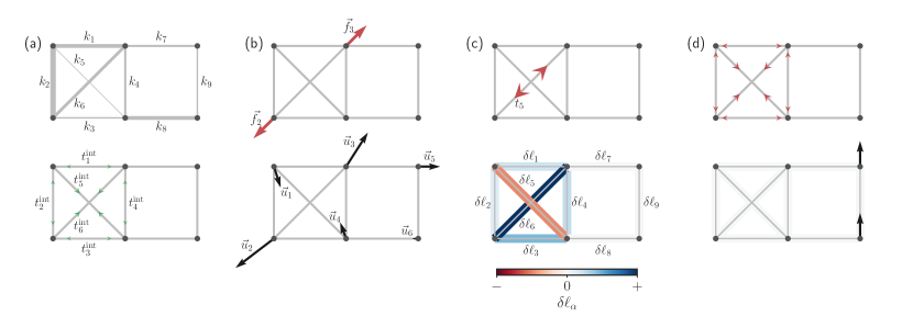
Figure 1: Local energetic properties, external perturbations, and elastic responses. The linear elastic properties are shown for a simple central-force spring network. (a) The stiffnesses of the bonds $k_{\alpha}$ (top), represented by line thickness, characterize their compressibility, while the prestress, or internal tensions, $t^{\mathrm{int}}_{\alpha}$ (bottom), characterize any geometric frustration that arises when the bond rest lengths force them to stretch or compress in the ground state configuration. Green arrows indicate the tension exerted by each bond on the rest of the network. (b) From the perspective of the nodes, external forces $\vec{f}_{i}$ (top) result in displacements $\vec{u}_{i}$ (bottom). The notation $\vec{u}_{i}$ and $\vec{f}_{i}$ represent the $d$-dimensional vectors of displacements and forces associated with each node $i$ for a network in $d$ dimensions. (c) From the perspective of the bonds, the external forces on the nodes are equivalent to external bond tensions $t_{\alpha}$ (top), while node displacements correspond to bond extensions $\delta\ell_{\alpha}$ (bottom) indicated by the color scale. (d) The network contains a state of self-stress (top) [identical to the prestress in (a)] composed of external tensions that result in no net forces on the nodes, along with a linear zero mode (bottom) composed of displacements that correspond to zero extension of the bonds.

II Elasticity Theory for Discrete Materials

In this section, we introduce the basic concepts and formalism we will use in the remainder of the paper. We consider a mechanical system consisting of $N_{\mathrm{c}}$ discrete components, each with size $\ell_{\alpha}(\{u_{i}\})$ (${\alpha=1,\ldots,N_{\mathrm{c}}}$), parameterized in terms of $N_{\mathrm{dof}}$ degrees of freedom $u_{i}$ (${i=1,\ldots,N_{\mathrm{dof}}}$). For convenience, we organize these quantities into the vectors $\vec{\boldsymbol{\ell}}$ and $\vec{\mathbf{u}}$, respectively. To evoke a concrete image, we will often discuss these quantities in the context of central-force spring networks in which the degrees of freedom are associated with the nodes, while the components are the springs, or bonds, defined by the edges of the network. For such a spring network with $n$ nodes in $d$ dimensions, $\vec{\mathbf{u}}$ is a $dn$-dimensional vector of node displacements, while $\vec{\boldsymbol{\ell}}$ is a $N_{\mathrm{c}}$-dimensional vector of bond lengths. Accordingly, we often refer to $\vec{\mathbf{u}}$ and $\vec{\boldsymbol{\ell}}$ as generalized “node displacements” and “bond lengths,” respectively.

Beyond central-force spring networks Lubensky et al. (2015), a broad range of systems in soft matter and biological physics may be cast in the above form. For example, in vertex models of biological tissues the generalized lengths $\vec{\boldsymbol{\ell}}$ may refer to the areas and perimeters of cells in a two-dimensional epithial tissue, or the cell volumes, surface areas, and edge lengths in a more general three-dimensional tissue Alt et al. (2017). Alternatively, the discrete components do not need to correspond to physical objects, but may be abstract in nature. Such examples include the lengths of bonds between neighboring particles in a jammed packing Liu and Nagel (2010), the angles associated with bond-bending costs between adjacent fiber segments in a biopolymer network Broedersz and MacKintosh (2014), or the angles between connected facets in an origami structure Schenk and Guest (2016). Similarly, the displacements $\vec{\mathbf{u}}$ may describe the change in any type degree of freedom from a system’s ground state, such as the orientational angles of particles that lack spherical symmetry like in jammed packings of elliptical particles Donev et al. (2007); Mailman et al. (2009).

II.1 Energy and external perturbations

We now write down the generalized Hamiltonian for these discrete materials. Defining $\vec{\mathbf{u}}=0$ as the system’s ground state in the absence of external perturbations, we measure changes in length via a set of generalized “bond extensions,” $\delta\vec{\boldsymbol{\ell}}(\vec{\mathbf{u}})\equiv\vec{\boldsymbol{\ell}}(\vec{\mathbf{u}})-\vec{\boldsymbol{\ell}}_{0}$, where $\vec{\boldsymbol{\ell}}_{0}\equiv\vec{\boldsymbol{\ell}}(0)$ are the “equilibrium lengths” of the bonds in the ground state.

At zero temperature, we consider the Hamiltonian

$$\mathcal{H}(\vec{\mathbf{u}})=E(\vec{\boldsymbol{\ell}}(\vec{\mathbf{u}}))+\frac{\lambda}{2}\norm*{\vec{\mathbf{u}}}^{2}-\vec{\mathbf{f}}\cdot\vec{\mathbf{u}}-\vec{\mathbf{t}}\cdot\delta\vec{\boldsymbol{\ell}}(\vec{\mathbf{u}}),$$ (1)

where the elastic energy $E(\vec{\boldsymbol{\ell}}(\vec{\mathbf{u}}))$ is expressed as a sum of the energetic costs of deforming each bond $\alpha$,

$$E(\vec{\boldsymbol{\ell}}(\vec{\mathbf{u}}))=\sum_{\alpha}V_{\alpha}(\ell_{\alpha}(\vec{\mathbf{u}});\ell^{*}_{\alpha}).$$ (2)

We introduce two externally applied generalized forces, $\vec{\mathbf{f}}$ and $\vec{\mathbf{t}}$, conjugate to the the displacements $\vec{\mathbf{u}}$ and bond lengths $\delta\vec{\boldsymbol{\ell}}(\vec{\mathbf{u}})$, respectively. By convention, we will often refer to $\vec{\mathbf{f}}$ as the external force and $\vec{\mathbf{t}}$ as the external tension. In general, we will be interested in linear response theory where these external perturbations are small.

We also add a small harmonic regularization term proportional to $\lambda$ which penalizes large displacements. This regularization serves as a convenient bookkeeping tool to keep track of deformations with no energetic cost (i.e., mechanisms or zero-energy modes). We will eventually be interested in the limit $\lambda\rightarrow 0$ where this term becomes negligible.

By convention, we define the rest length $\ell^{*}_{\alpha}$ for each bond such that ${V_{\alpha}(\ell^{*}_{\alpha};\ell^{*}_{\alpha})=0}$ (in general, $\ell^{*}_{\alpha}$ may differ from $\ell_{0,\alpha}$). For example, in a harmonic spring network, the potentials take the form ${V_{\alpha}(\ell_{\alpha}(\vec{\mathbf{u}});\ell^{*}_{\alpha})=\frac{1}{2}k_{\alpha}(\ell_{\alpha}(\vec{\mathbf{u}})-\ell^{*}_{\alpha})^{2}}$ where $k_{\alpha}$ is the stiffness of bond $\alpha$.

To determine the elastic response, we minimize Eq. (1) with respect to the displacements by setting its gradient to zero,

$$0=\partialderivative{\mathcal{H}(\vec{\mathbf{u}})}{u_{i}},$$ (3)

and then solve the resulting $N_{\mathrm{dof}}$ equations for the resulting displacements $\vec{\mathbf{u}}$.

II.2 Local energetic properties in the linear regime

In the linear regime, the elastic energy [Eq. (2)] close to the ground state is characterized by the Hessian $\mathbf{H}$, given by

$$H_{ij} =\partialderivative{E}{u_{i}}{u_{j}}\evaluated{}_{\vec{\mathbf{u}}=0}$$ (4)

$$=\sum_{\alpha\beta}\partialderivative{\ell_{\alpha}}{u_{i}}K_{\alpha\beta}\partialderivative{\ell_{\beta}}{u_{j}}+\sum_{\alpha}t^{\mathrm{int}}_{\alpha}\partialderivative{\ell_{\alpha}}{u_{i}}{u_{j}},$$

with

$$t^{\mathrm{int}}_{\alpha}=\partialderivative{E}{\ell_{\alpha}}=V^{\prime}_{\alpha},$$ (5)

$$K_{\alpha\beta}=\partialderivative{E}{\ell_{\alpha}}{\ell_{\beta}}=V^{\prime\prime}_{\alpha}\delta_{\alpha\beta}=k_{\alpha}\delta_{\alpha\beta}.$$ (6)

The vector of prestresses (internal tensions) $\vec{\mathbf{t}}^{\mathrm{int}}$ and the stiffness matrix $\mathbf{K}$ encode the system’s local energetic properties in the linear regime. While the stiffness $k_{\alpha}$ describes the energetic cost of deforming bond $\alpha$, the prestress $t^{\mathrm{int}}_{\alpha}$ describes any frustration arising due to incompatibility between a bond’s rest length and its equilibrium length in the system’s global ground state (${\ell^{*}_{\alpha}\neq\ell_{0,\alpha}}$). As an example, in a harmonic spring network, prestress takes the form ${t^{\mathrm{int}}_{\alpha}=k_{\alpha}(\ell_{0,\alpha}-\ell^{*}_{\alpha})}$.

In Fig. 1(a), we demonstrate possible values of the stiffness and prestresss for a simple central-force harmonic spring network. To achieve the prestress depicted in this ground state configuration, we assign incompatible rest lengths to bonds 1-6 so that the four outer bonds (1-4) are compressed in the ground state, $\ell_{0,\alpha}<\ell_{\alpha}^{*}$, while the two diagonal bonds (5-6) are stretched, $\ell_{0,\alpha}>\ell_{\alpha}^{*}$. This creates frustration that cannot be relaxed away by moving the nodes.

II.3 Node space and bond space representations

In general, it is helpful to think about the linear response in two difference spaces, node space (degrees of freedom) and bond space (components or constraints). In node space, applying a set of forces $\vec{\mathbf{f}}$ to nodes results in a set of displacements $\vec{\mathbf{u}}$. An example of this is shown in Fig. 1(b), where external applied forces (top) result in displacements of the nodes (bottom). Alternatively, we can think about how these quantities in node space correspond to their counterparts in bond space, i.e., tensions and extensions. In Fig. 1(c), we depict a set of bonds tensions $\vec{\mathbf{t}}$ (top) that result in the same set of displacements as the forces in Fig. 1(b), along with the bond extensions $\delta\vec{\boldsymbol{\ell}}$ (bottom) resulting from those displacements. Intuitively, it is clear that every set of external tensions should be equivalent to some set of external forces, while each set of displacements should result in a unique set of bond extensions.

In the linear regime, the correspondence between quantities in node space and bond space is provided by the compatibility matrix $\mathbf{C}$ (or equivalently, the equilibrium matrix $\mathbf{C}^{T}$), defined as

$$C_{\alpha i}=\partialderivative{\ell_{\alpha}}{u_{i}}\evaluated{}_{\vec{\mathbf{u}}=0},$$ (7)

through the relations

$$\delta\vec{\boldsymbol{\ell}}=\mathbf{C}\vec{\mathbf{u}},\qquad\vec{\mathbf{f}}=\mathbf{C}^{T}\vec{\mathbf{t}}.$$ (8)

The first relation between the extensions and displacements is simply a result of the chain rule. The second relation between external tensions and forces requires a slightly more subtle argument. Expanding the tension term in Eq. (1) to linear order in $\vec{\mathbf{u}}$, we get

$$\vec{\mathbf{t}}\cdot\delta\vec{\boldsymbol{\ell}}(\vec{\mathbf{u}})\approx\sum_{i}\vec{\mathbf{t}}\cdot\partialderivative{\vec{\boldsymbol{\ell}}}{u_{i}}\evaluated{}_{\vec{\mathbf{u}}=0}u_{i}=(\mathbf{C}^{T}\vec{\mathbf{t}})\cdot\vec{\mathbf{u}}.$$ (9)

Comparing this expression with the force term in Eq. (1), $\vec{\mathbf{f}}\cdot\vec{\mathbf{u}}$, we see that applying an external tension $\vec{\mathbf{t}}$ to the bonds is equivalent to applying a force $\vec{\mathbf{f}}=\mathbf{C}^{T}\vec{\mathbf{t}}$ to the nodes.

II.4 The simplest case: zero prestress with uniform stiffness

Throughout this paper, it will be instructive to examine the elastic response in the particularly simple case of zero prestress $\vec{\mathbf{t}}^{\mathrm{int}}=0$ with uniform unit bond stiffness ${\mathbf{K}=\mathbf{I}}$. It is within this setting that the Maxwell-Calladine framework is typically derived Lubensky et al. (2015). In this special case, the Hessian [Eq. (4)] attains the simple form

$$\mathbf{H}=\mathbf{C}\mathbf{C}^{T}.$$ (10)

Essentially, when the energetic properties are trivial, the Hessian contains the same information as the compatibility matrix $\mathbf{C}$. In other words, deformations are completely characterized by the system’s geometry encoded in $\mathbf{C}$. However, in more general situations – such as in the presence of prestress or heterogeneous bond stiffnesses – the Hessian and its associated elastic response will also depend on the precise details of the energetic properties encoded in $\mathbf{K}$ and $\vec{\mathbf{t}}^{\mathrm{int}}$.

II.5 Maxwell-Calladine Index Theorem

We now present a brief derivation of the classic Maxwell-Calladine index theorem with an eye to generalizing it to include prestress and heterogeneous bond stiffness. In the Maxwell-Calladine framework, a central role is played by the compatibility matrix $\mathbf{C}$. The compatibility matrix relates quantities which reside in the $N_{\mathrm{c}}$-dimensional bond space to those that live in the $N_{\mathrm{dof}}$-dimensional node space. According to Eq. (8), $\mathbf{C}$ is formally a linear map from displacements in node space $\vec{\mathbf{u}}$ to extensions in bond space $\vec{\boldsymbol{\ell}}$, while $\mathbf{C}^{T}$ is a linear map from tensions $\vec{\mathbf{t}}$ in bond space to forces in node space $\vec{\mathbf{f}}$.

Applying rank-nullity theorem, we can express the dimension of the domain of each operator as the sum of its rank plus the dimension of its kernel (right null space). According to Eq. (8), the kernel of $\mathbf{C}$ is composed of linear zero modes (LZMs), or displacements that do not extend or compress the bonds to linear order. Thus, we have

$$N_{\mathrm{dof}}=\mathrm{rank}(\mathbf{C})+\mathrm{\#LZMs}.$$ (11)

Analogously, the kernel of $\mathbf{C}^{T}$ is composed of states of self-stress (SSSs), or tensions that balance to create zero net forces on the nodes, and we have

$$N_{\mathrm{c}}=\mathrm{rank}(\mathbf{C}^{T})+\mathrm{\#SSSs}.$$ (12)

Because $\mathbf{C}$ and $\mathbf{C}^{T}$ are transposes of one another, their ranks are equal. Using this observation, we subtract the second equation from the first, yielding the Maxwell-Calladine index theorem,

$$N_{\mathrm{dof}}-N_{\mathrm{c}}=\mathrm{\#LZMs}-\mathrm{\#SSSs},$$ (13)

relating the difference in the number of degrees of freedom and constraints to the difference in the number of LZMs and SSSs. Based on Eq. (13), one concludes a system is rigid to first order when the number of LZMs is zero (excluding global translations and rotations, if applicable).

As an illustration, we analyze the rigidity of the network in Fig. 1, which has six nodes in two dimensions for a total of $N_{\mathrm{dof}}=12$ degrees of freedom and $N_{\mathrm{c}}=9$ bonds that impose constraints on the system. This network also has one SSS, shown in the top of Fig. 1(d), which happens to be identical to the prestress in Fig. 1(b) (the prestress $\vec{\mathbf{t}}^{\mathrm{int}}$ is always a SSS since in the ground state ${0=\partialderivative{E}{\vec{\mathbf{u}}}=\mathbf{C}^{T}\vec{\mathbf{t}}^{\mathrm{int}}}$). Solving Eq. (13), we find that this network should have four LZMs. Since two of these modes correspond to global translations along the $x-$ and $y-$ axes and one to a global rotation, there must be one additional LZM, shown in the bottom of Fig. 1(d). Thus, we conclude that the system is not rigid to first order.

III Elastic Susceptibilities

The derivation of Maxwell-Calladine is based exclusively on the geometry encoded in the compatibility matrix $\mathbf{C}$, ignoring prestress and stiffness. To incorporate these energetic properties and derive a generalized index theorem, it is necessary to assess a system’s rigidity directly via its response to external perturbations, rather than indirectly via the geometry. The response of a discrete material can be characterized by four distinct susceptibility matrices that measure how displacements and extensions respond to externally applied forces and tensions. These susceptibilities play a central role in what follows and are the key physical objects necessary to generalize the Maxwell-Calladine framework to include energetics.

III.1 Definitions and expressions for susceptibilities

The natural objects of all linear response theories are susceptibilities that characterize how the system responds to external perturbations. As hinted by our choice of Hamiltonian in Eq. 1, we will focus on the response of the system to the application of external forces $\vec{\mathbf{f}}$ and tensions $\vec{\mathbf{t}}$. The response can be characterized either in terms of the displacements $\vec{\mathbf{u}}$ or extensions $\delta\vec{\boldsymbol{\ell}}$. This results in four distinct yet related matrix susceptibilities:

$$\quantity[\partialderivative{\vec{\mathbf{u}}}{\vec{\mathbf{f}}}]_{ij} =\partialderivative{u_{i}}{f_{j}}, \quantity[\partialderivative{\vec{\mathbf{u}}}{\vec{\mathbf{t}}}]_{i\beta} =\partialderivative{u_{i}}{t_{\beta}},$$ (14)

$$\quantity[\partialderivative{\vec{\boldsymbol{\ell}}}{\vec{\mathbf{f}}}]_{\alpha j} =\partialderivative{\ell_{\alpha}}{f_{j}}, \quantity[\partialderivative{\vec{\boldsymbol{\ell}}}{\vec{\mathbf{t}}}]_{\alpha\beta} =\partialderivative{\ell_{\alpha}}{t_{\beta}}.$$

It will be helpful to subdivide these four susceptibilities into the two square “diagonal” susceptibilities, $\partialderivative{\vec{\mathbf{u}}}{\vec{\mathbf{f}}}$ and $\partialderivative{\vec{\boldsymbol{\ell}}}{\vec{\mathbf{t}}}$, which map between spaces of the same dimensions and the two rectangular “off-diagonal” susceptibilities, $\partialderivative{\vec{\mathbf{u}}}{\vec{\mathbf{t}}}$ and $\partialderivative{\vec{\boldsymbol{\ell}}}{\vec{\mathbf{f}}}$, that map between spaces of different dimensions.

To derive explicit expressions for these susceptibilities, we take advantage of the fact that we are looking at perturbations of minimum energy configurations that obey the $N_{\mathrm{dof}}$ equations of Eq. (3). We differentiate these equations with respect to $f_{j}$ and solve the resulting matrix equations to obtain an explicit expression for $\partialderivative{\vec{\mathbf{u}}}{\vec{\mathbf{f}}}$. The other susceptibilities are then derived from $\partialderivative{\vec{\mathbf{u}}}{\vec{\mathbf{f}}}$ using the chain rule. As shown in the appendix, in the limit $\lambda\rightarrow 0$, the four susceptibilities are

$$\partialderivative{\vec{\mathbf{u}}}{\vec{\mathbf{f}}} =\mathbf{H}^{+}+\frac{1}{\lambda}\mathbf{P}_{H}^{\mathrm{ZEM}}, \partialderivative{\vec{\mathbf{u}}}{\vec{\mathbf{t}}} =\partialderivative{\vec{\mathbf{u}}}{\vec{\mathbf{f}}}\mathbf{C}^{T},$$ (15)

$$\partialderivative{\vec{\boldsymbol{\ell}}}{\vec{\mathbf{f}}} =\mathbf{C}\partialderivative{\vec{\mathbf{u}}}{\vec{\mathbf{f}}}, \partialderivative{\vec{\boldsymbol{\ell}}}{\vec{\mathbf{t}}} =\mathbf{C}\partialderivative{\vec{\mathbf{u}}}{\vec{\mathbf{f}}}\mathbf{C}^{T},$$

where $\mathbf{H}^{+}$ is the Moore-Penrose inverse, or pseudoinverse, of the Hessian and ${\mathbf{P}^{\mathrm{ZEM}}_{H}=\mathbf{I}-\mathbf{H}\mathbf{H}^{+}}$ is an orthogonal projector onto its kernel, containing the zero energy modes of the Hessian.

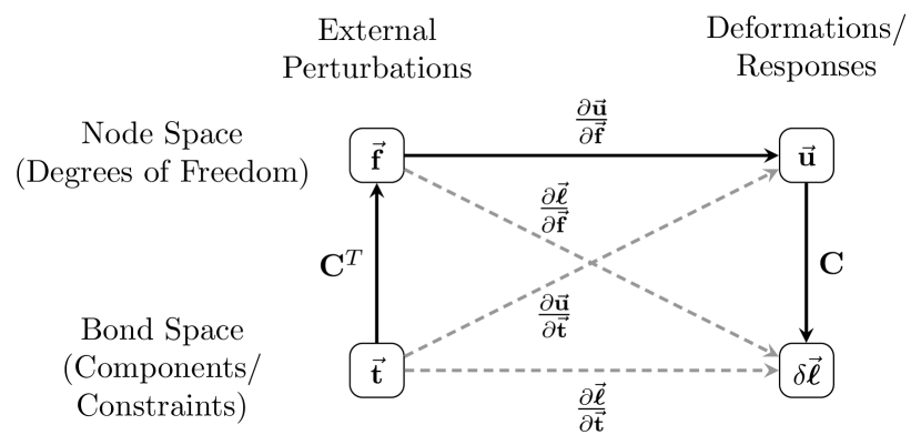
Figure 2: Susceptibilities and their relationships as maps between spaces. The four susceptibilities, the compatibility matrix, and its transpose allow either forces and tensions to be mapped to either displacements and extensions. While, $\mathbf{C}$ and $\mathbf{C}^{T}$ provide maps between node space (degrees of freedom) (top row) bond space (components/constraints) (bottom row), the susceptibilities provide maps from external perturbations (left column) to deformation responses (right column). Arrows indicate the direction of each map with dashed arrows representing operators that are compositions of other operators.

III.2 Susceptibilities as maps between spaces

In our formalism, a privileged role is played by the diagonal susceptibility $\partialderivative{\vec{\mathbf{u}}}{\vec{\mathbf{f}}}$. Physically, $\partialderivative{\vec{\mathbf{u}}}{\vec{\mathbf{f}}}$ is linear map from external forces to the resulting displacements of the nodes. To gain intuition about this suspectibility, it is helpful to examine the explicit expression for $\partialderivative{\vec{\mathbf{u}}}{\vec{\mathbf{f}}}$ in Eq. (15). The expressions is composed of two parts: the pseudoinverse of the Hessian $\mathbf{H}^{+}$ and the projection operator $\mathbf{P}_{H}^{\mathrm{ZEM}}$. The pseudoinverse $\mathbf{H}^{+}$ simply describes harmonic motion of the degrees of freedom around their minimum energy positions in rigid directions (i.e., directions in which the Hessian has nonzero eigenvalues). On the other hand, the projection operator $\mathbf{P}_{H}^{\mathrm{ZEM}}$ describes motions resulting from exciting modes that cost zero energy (i.e., eigenmodes of the Hessian with eigenvalues of zero). Furthermore, notice that the projector term is proportional to $\lambda^{-1}$. Thus, in the physical limit without regularization, $\lambda\rightarrow 0$, forces that excite these zero energy modes result in unconstrained displacements with magnitudes that diverge as $\lambda^{-1}$.

More generally, the four susceptibilities in Eq. (15) combine with $\mathbf{C}$ and $\mathbf{C}^{T}$ to form a set of linear operators that can be composed to map either type of external perturbation ($\vec{\mathbf{f}}$ or $\vec{\mathbf{t}}$) to either type of deformation ($\vec{\mathbf{u}}$ or or $\delta\vec{\boldsymbol{\ell}}$). We illustrate their relationships graphically in Fig. 2. While $\mathbf{C}$ relates deformations in node space (displacements) to those in bond space (extensions) and $\mathbf{C}^{T}$ relates external perturbations in bond space (tensions) to those in node space (forces) via Eq. 8, the susceptibilities always relate external perturbations to deformations. In this picture, $\mathbf{C}$, $\mathbf{C}^{T}$, and $\partialderivative{\vec{\mathbf{u}}}{\vec{\mathbf{f}}}$ can be viewed as a set of “fundamental” operators (shown with solid arrows) whose compositions give rise to the remaining three susceptibilities (shown with dashed arrows).

III.3 Collective mode taxonomy

Just as the original Maxwell-Calladine theorem relates collective modes in the kernels of $\mathbf{C}$ and $\mathbf{C}^{T}$, our generalized index theorem will relate modes in the kernels of $\partialderivative{\vec{\mathbf{u}}}{\vec{\mathbf{t}}}$ and $\partialderivative{\vec{\boldsymbol{\ell}}}{\vec{\mathbf{f}}}$. For this reason, it is worth briefly summarizing our nomenclature for these collective modes, as well as their physical meanings. As discussed earlier in the context of the Maxwell-Calladine theorem, the spaces spanned by the kernels of $\mathbf{C}$ and $\mathbf{C}^{T}$ are usually referred to as linear zero modes (LZMs) and states of self-stress (SSS), respectively. The Maxwell-Calladine theorem relates the dimensions of these two spaces to the numbers of degrees of freedom and constraints.

In our generalized mode taxonomy, an analogous role will be played by the modes that span the kernels of $\partialderivative{\vec{\mathbf{u}}}{\vec{\mathbf{t}}}$ and $\partialderivative{\vec{\boldsymbol{\ell}}}{\vec{\mathbf{f}}}$. We note that both of these types of modes correspond to external perturbations. Physically, modes that lie in the kernel of $\partialderivative{\vec{\boldsymbol{\ell}}}{\vec{\mathbf{f}}}$ correspond to nontrivial sets of external forces $\vec{\mathbf{f}}$ that may displace the nodes, but do not actually extend the bonds. We will refer to these modes as linear zero-extension forces (LZEFs). Similarly, modes that lie in the kernel of $\partialderivative{\vec{\mathbf{u}}}{\vec{\mathbf{t}}}$ correspond to sets of external tensions that do not result in any displacement of the nodes when applied to the bonds. We will refer to these modes as zero displacement tensions (ZDTs). See Table 1 for a summary of this collective mode taxonomy.

Table 1: Collective Mode Taxonomy

Operator : Domain $\rightarrow$ Codomain	Kernel
$\mathbf{C}:$ Displacements $\rightarrow$ Extensions	Linear Zero Modes (LZM)
$\mathbf{C}^{T}:$ Tensions $\rightarrow$ Forces	States of Self-Stress (SSS)
$\partialderivative{\vec{\mathbf{u}}}{\vec{\mathbf{t}}}:$ Tensions $\rightarrow$ Displacements	Zero-Displacement Tensions (ZDT)
$\partialderivative{\vec{\boldsymbol{\ell}}}{\vec{\mathbf{f}}}:$ Forces $\rightarrow$ Extensions	Linear Zero-Extension Forces (LZEF)

IV Generalized Index Theorem

We are now in a position to derive a generalization of the Maxwell-Calladine index theorem. Importantly, our generalized index theorem holds even in the presence of nonzero prestress or heterogeneous bond stiffnesses. We focus on the two off-diagonal susceptibilities relating node and bond space, $\partialderivative{\vec{\mathbf{u}}}{\vec{\mathbf{t}}}$ and $\partialderivative{\vec{\boldsymbol{\ell}}}{\vec{\mathbf{f}}}$. Following a procedure analogous to the derivation in Sec. II.5, we apply rank-nullity theorem to express the dimension of the domain of each operator as a sum of its rank plus the dimension of its kernel. Using the definitions of LZEFs and ZDTs from the previous section as the collective modes in the kernels of the two susceptibilities, we obtain

$$N_{\mathrm{dof}} =\mathrm{rank}\quantity(\partialderivative{\vec{\boldsymbol{\ell}}}{\vec{\mathbf{f}}})+\mathrm{\#LZEFs},$$ (16)

$$N_{\mathrm{c}} =\mathrm{rank}\quantity(\partialderivative{\vec{\mathbf{u}}}{\vec{\mathbf{t}}})+\mathrm{\#ZDTs}.$$ (17)

Since the two susceptibilities are transposes of one another [see Eq. (15)], their ranks are equal. Using this fact, we subtract the second equation from the first to arrive at our generalized index theorem,

$$N_{\mathrm{dof}}-N_{\mathrm{c}}=\mathrm{\#LZEFs}-\mathrm{\#ZDTs}.$$ (18)

Comparing to the classic version in Eq. (13), we see that the left hand side is identical, containing the difference in the number of degrees of freedoms and constraints, while the right hand side now contains the difference in the number of LZEFS and ZDTs. At first glance, these modes seem to be very different from those usually considered in the Maxwell-Calladine theorem, namely LZMs and SSSs. Whereas LZMs and SSSs are purely properties of the system’s geometry encoded by $\mathbf{C}$ and $\mathbf{C}^{T}$, LZEFS and ZDTs are types of external perturbations which depend on both the system’s geometry and local energetics (prestress and stiffness). We will see that these two sets of modes are intimately related and can even be shown to be equivalent in special cases depending on the precise details of the energy.

V Collective Mode Relationships

In this section, we explore the relationship between the collective modes of the Maxwell-Calladine index theorem (SSSs and LZMs) and their counterparts in the generalized version (ZDTs and LZEFs). We first demonstrate this relationship explicitly in the simple case discussed in Sec. II.4 where the details of the energetic properties can essentially be ignored (i.e., zero prestress and uniform bond stiffness). We then move on to the general case of arbitrary local energetic properties where we formalize these results into a pair of theorems.

V.1 The simplest case: zero prestress with uniform stiffness

In the case of zero prestress, $\vec{\mathbf{t}}^{\mathrm{int}}=0$, with uniform unit stiffness, $\mathbf{K}=\mathbf{I}$, the susceptibility $\partialderivative{\vec{\mathbf{u}}}{\vec{\mathbf{f}}}$ takes on an especially simple form. Combining Eqs. (10) and  (15), and using properties of the pseudoinverse, we obtain

$$\partialderivative{\vec{\mathbf{u}}}{\vec{\mathbf{f}}}=\quantity[\mathbf{C}^{T}\mathbf{C}]^{+}+\frac{1}{\lambda}\quantity[\mathbf{I}-\mathbf{C}^{+}\mathbf{C}],$$ (19)

where to reiterate, the first term is the pseudoinverse of the Hessian and the second term is a projector onto the zero energy modes. According to Eq. (15), we then appropriately multiply by $\mathbf{C}$ or $\mathbf{C}^{T}$ to obtain simplified forms for the two off-diagonal susceptibilities,

$$\partialderivative{\vec{\mathbf{u}}}{\vec{\mathbf{t}}}=\mathbf{C}^{+},\qquad\partialderivative{\vec{\boldsymbol{\ell}}}{\vec{\mathbf{f}}}=\quantity[\mathbf{C}^{+}]^{T}.$$ (20)

When taking the pseudoinverse of a general rectangular matrix such as $\mathbf{C}$, the row and column spaces of the matrix are swapped, along with the left and right null spaces. Thus, the kernel of $\partialderivative{\vec{\mathbf{u}}}{\vec{\mathbf{t}}}$ is the same as $\mathbf{C}^{T}$ and similarly, the kernel of $\partialderivative{\vec{\boldsymbol{\ell}}}{\vec{\mathbf{f}}}$ is the same as $\mathbf{C}$. In other words, for the simple case of zero prestress with uniform stiffness, the two index theorems provide identical information: the SSSs and LZMs are the same as the ZDTs and LZEFs, respectively!

To make this connection more transparent, we take advantage of the fact that the susceptibility $\partialderivative{\vec{\mathbf{u}}}{\vec{\mathbf{f}}}$ is guaranteed to be full rank and is therefore invertible. While $\partialderivative{\vec{\mathbf{u}}}{\vec{\mathbf{f}}}$ uniquely maps external forces to their resulting displacements, its inverse $\quantity[\partialderivative{\vec{\mathbf{u}}}{\vec{\mathbf{f}}}]^{-1}$ uniquely maps displacements to the external forces that created them.

Now consider a LZEF $\vec{\mathbf{f}}^{\mathrm{LZEF}}$. Since LZEFs do not extend the bonds, the displacement created by $\vec{\mathbf{f}}^{\mathrm{LZEF}}$ must preserve the bond lengths as well. Thus, every LZEF $\vec{\mathbf{f}}^{\mathrm{LZEF}}$ results in a displacement along a LZM $\vec{\mathbf{u}}^{\mathrm{LZM}}$ given by

$$\vec{\mathbf{u}}^{\mathrm{LZM}}=\partialderivative{\vec{\mathbf{u}}}{\vec{\mathbf{f}}}\vec{\mathbf{f}}^{\mathrm{LZEF}}.$$ (21)

Because $\partialderivative{\vec{\mathbf{u}}}{\vec{\mathbf{f}}}$ is invertible, we may also solve the above equation for a fixed LZM to find the unique LZEF that couples to it. In short, the LZMs and LZEFs are isomorphic, related by the map provided by $\partialderivative{\vec{\mathbf{u}}}{\vec{\mathbf{f}}}$.

For the case of zero prestress and uniform stiffness, Eq. (21) is especially simple. Using Eqs. (19) and (20), combined with the the definition of a LZEF, ${\partialderivative{\vec{\boldsymbol{\ell}}}{\vec{\mathbf{f}}}\vec{\mathbf{f}}^{\mathrm{LZEF}}=0}$, we find

$$\vec{\mathbf{u}}^{\mathrm{LZM}}=\frac{1}{\lambda}\vec{\mathbf{f}}^{\mathrm{LZEF}}.$$ (22)

Thus, in this simple case, each LZEF couples to a LZM that is the same up to a constant prefactor. Furthermore, the prefactor of $\lambda^{-1}$ indicates that all LZMs also happen to be zero energy modes in this case.

The relationship between ZDTs and SSSs is even more straightforward since they are both types of external tensions. Now note that by definition, a SSS does not generate net forces on the nodes. Because $\partialderivative{\vec{\mathbf{u}}}{\vec{\mathbf{f}}}$ is full rank and uniquely map from forces to displacements, the zero net force created by a SSS must also result in zero displacement of the nodes. Similarly, because a ZDT does not generate displacements, applying $\quantity[\partialderivative{\vec{\mathbf{u}}}{\vec{\mathbf{f}}}]^{-1}$ maps the zero displacement created by a ZDT to zero net forces on the nodes. Thus, we conclude that every SSS is a ZDT and every ZDT is a SSS. Evidently, the two types of modes are always equivalent.

V.2 Collective Mode Correspondence Theorems

We formulate the observations from the previous section into two theorems. Proofs for both theorems are provided in the Appendix. First, the following theorem describes the general correspondence between the different types of modes:

Theorem 1.

Suppose a system is described by the Hamilton in Eq. (1). Then the following is true:

1. The ZDTs and SSSs are equivalent.

2. The LZEFs are isomorphic to the LZMs, with each LZEF $\vec{\mathbf{f}}^{\mathrm{LZEF}}$ coupling to a unique LZM $\vec{\mathbf{u}}^{\mathrm{LZM}}$ according to the bijective map

   $$\vec{\mathbf{u}}^{\mathrm{LZM}}=\partialderivative{\vec{\mathbf{u}}}{\vec{\mathbf{f}}}\vec{\mathbf{f}}^{\mathrm{LZEF}}.$$ (23)

We emphasize that in general, the LZEFs and LZMs span different subspaces of the $N_{\mathrm{dof}}$-dimensional node space. The precise correspondence between these two types of collective modes depends on the interplay of the system’s geometric structure and its local energetic properties encoded in the susceptibility $\partialderivative{\vec{\mathbf{u}}}{\vec{\mathbf{f}}}$.

In the previous section, we saw that for zero prestress and uniform stiffness, the LZEFs and LZMs were identical – each LZEF couples to a displacement along a parallel LZM [Eq. (22)]. While this case is especially simple, it can be shown that such mode equivalence generalizes to a much broader class of systems described by the following theorem:

Theorem 2.

Suppose the elastic response of a discrete material is described by the Hamilton in Eq. (1). Define the prestress matrix $\mathbf{T}$ with elements

$$T_{ij}=\sum_{\alpha}t^{\mathrm{int}}_{\alpha}\partialderivative{\ell_{\alpha}}{u_{i}}{u_{j}}.$$ (24)

If the following commutation relation holds:

$$\commutator{\mathbf{C}^{T}\mathbf{C}}{\mathbf{T}}=0,$$ (25)

then the LZEFs and LZMs span the same vector space.

Based on this theorem, it becomes clear that in the absence of prestress, $\vec{\mathbf{t}}^{\mathrm{int}}=0$, Eq. (25) holds irrespective of the stiffness matrix $\mathbf{K}$. Furthermore, it can be shown that when this theorem is satisfied, the LZEFs and LZMs may be represented in the same basis such that each LZEF couples to a unique parallel LZM, resulting in a generalization of Eq. (22) (see Corollary 1 in Appendix).

VI Symmetry Breaking with Local Energy Costs

In this section, we explore how a system’s local energetic properties may be used to control the relationship between LZEFs the LZMs to which they couple. According to Theorem 2 the LZEFs and LZMs are guarenteed to match as long as the compatibility (squared) matrix $\mathbf{C}^{T}\mathbf{C}$ and the prestress matrix $\mathbf{T}$ commute according to Eq. (25). A basic property of two commuting matrices is that they are simultaneously diagonalizable, or can be decomposed with the same basis of eigenvectors.

Throughout the field of physics, a classic situation in which two operators commute is when they both exhibit the same symmetries, or are invariant under transformations of the symmetry group Zee (2016). For a discrete material that obeys Eq. (25), this means the geometrical structure encoded in the compatibility matrix $\mathbf{C}$ must exhibit the same symmetries as the local energetics (prestress) and geometry encoded in $\mathbf{T}$. Using simple examples, we will demonstrate how this idea may be exploited to design metamaterials with specific responses. Specifically, we will use prestress to either break or preserve symmetries in a system’s geometry to control the coupling between LZEFs to LZMs.

VI.1 Energy-Geometry Symmetry Matching Theorem

Before moving on, we first use group representation theory Zee (2016) to formulate this design principle into the following theorem:

Theorem 3.

Suppose a system is described by the Hamiltonian in Eq. (1). Let $G$ be a finite symmetry group with two unitary matrix representations, ${\mathbf{D}^{(u)}:G\rightarrow\mathrm{GL}(\mathbb{R}^{N_{\mathrm{dof}}})}$ and ${\mathbf{D}^{(\delta\ell)}:G\rightarrow\mathrm{GL}(\mathbb{R}^{N_{\mathrm{c}}})}$, that act on node space and bond space, respectively [$\mathrm{GL}(\mathcal{V})$ is the general linear group of the vector space $\mathcal{V}$]. If a system is invariant under the symmetry transformations of $G$ such that for every $g\in G$, its bond lengths and node displacements obey the invariance relation

$$\vec{\boldsymbol{\ell}}(\vec{\mathbf{u}})=\mathbf{D}^{(\delta\ell)}(g^{-1})\vec{\boldsymbol{\ell}}\quantity(\mathbf{D}^{(u)}(g)\vec{\mathbf{u}})$$ (26)

and its energy obeys the invariance relation

$$E(\vec{\boldsymbol{\ell}}(\vec{\mathbf{u}}))=E\quantity(\mathbf{D}^{(\delta\ell)}(g)\vec{\boldsymbol{\ell}}(\vec{\mathbf{u}})),$$ (27)

then the LZEFs and LZMs span the same vector space.

In the linear regime, the invariance relation Eq. (26) implies that the system exhibits geometric symmetry. Mathematically, this means that the compatibility matrix is invariant under actions of the the symmetry group with invariance relation

$$\mathbf{C}=\mathbf{D}^{(\delta\ell)}(g^{-1})\mathbf{C}\mathbf{D}^{(u)}(g)$$ (28)

(with an analogous relationship for $\partialderivative{\ell_{\alpha}}{u_{i}}{u_{i}}$). Meanwhile, Eq. (27) implies that the local energetic costs of deforming each bond also exhibit the same symmetry. Mathematically, the stiffesses and prestress are invariant according to

$$\vec{\mathbf{t}}^{\mathrm{int}} =\mathbf{D}^{(\delta\ell)}(g)\vec{\mathbf{t}}^{\mathrm{int}}$$ (29)

$$\mathbf{K} =\mathbf{D}^{(\delta\ell)}(g^{-1})\mathbf{K}\mathbf{D}^{(\delta\ell)}(g).$$ (30)

When both the network’s geometric structure and local energetic properties are invariant under transformations of same symmetry group, then both $\mathbf{C}^{T}\mathbf{C}$ and $\mathbf{T}$ will also be invariant commute according to Eq. (25) (see Appendix for proof).

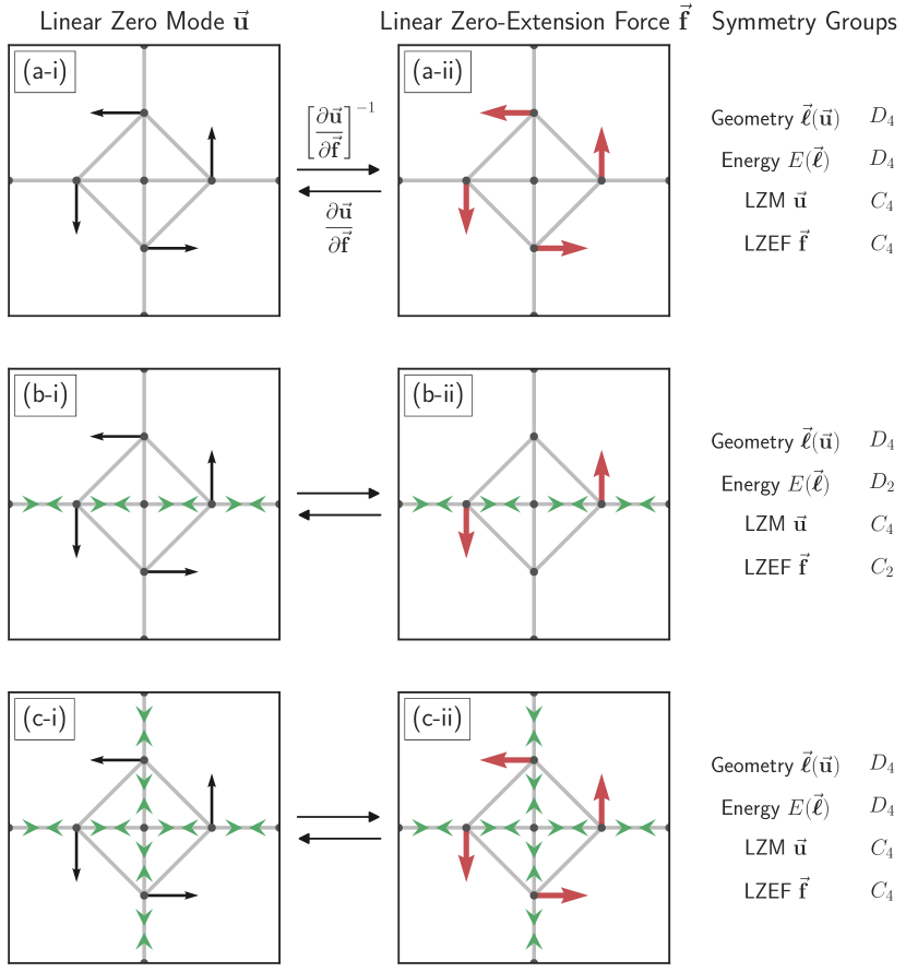
Figure 3: Breaking rotational symmetry with prestress. A periodic central-force spring network whose geometry exhibits fourfold dihedral symmetry ($D_{4}$). In each row, a linear zero mode (LZM) and the linear zero-extension force (LZEF) that couples to it via the susceptibility $\partialderivative{\vec{\mathbf{u}}}{\vec{\mathbf{f}}}$ are shown for a different choice of prestress. The rightmost column lists the symmetry groups for each case describing the geometry, energy (prestress), LZM,and LZEF. In all cases, the spring constants are chosen to be uniform ($\mathbf{K}=\mathbf{I}$). (a) When the prestress is zero ($\vec{\mathbf{t}}^{\mathrm{int}}=0$) the energy exhibits the same symmetry as the geometry. The (a-i) LZM and its corresponding (a-ii) LZEF are identical, both exhibiting fourfold rotational symmetry ($C_{4}\subset D_{4}$). (b) Introducing nonzero prestress along the central line of horizontal bonds breaks the energetic symmetry from fourfold to twofold dihedral symmetry ($D_{2}\subset D_{4}$). While the (b-i) LZM is the same, the (b-ii) LZEF that couples to it no longer matches, exhibiting twofold rotational symmetry ($C_{2}\subset C_{4}$). (c) Introducing additional prestress along the central line of vertical bonds restores the fourfold dihedral symmetry to the energy. The (c-i) LZM and the (c-ii) LZM that couples to it match once again.

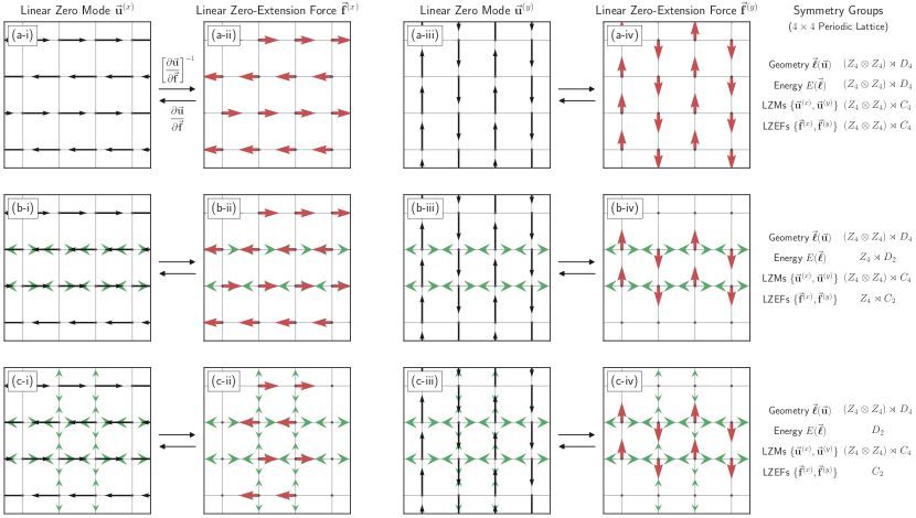
Figure 4: Breaking translational symmetry subgroups with prestress. A central-force spring network consiting of a $4\times 4$ periodic lattice. The network geoemtry exhibits fourfold dihedral symmetry, along with discrete translational symmetry along the $x$- and $y$-axes [$(Z_{4}\otimes Z_{4})\rtimes D_{4}$]. In each row, two linear zero modes (LZMs) and the linear zero-extension forces (LZEFs) that couple to them via the susceptibility $\partialderivative{\vec{\mathbf{u}}}{\vec{\mathbf{f}}}$ are shown for a different choice of prestress. The rightmost column lists the symmetry groups for each case describing the geometry, energy (prestress), LZMs, and LZEFs. In all cases, the spring constants are chosen to be uniform ($\mathbf{K}=\mathbf{I}$). (a) For zero prestress ($\vec{\mathbf{t}}^{\mathrm{int}}=0$) the energy and geometry exhibit the same symmetry. Each LZM matches the LZEF that couples to it, with one pair, (a-i) and (a-ii), exhibiting translational symmetry along the $x$-axis, and the other pair, (a-iii) and (a-iv), exhibiting translational symmetry along the $y$-axis. (b) Introducing nonzero prestress along two horizontal lines of bonds breaks the $y$-translational symmetry of the energy ($Z_{4}\rtimes D_{2}$). The (b-iv) LZEF that previously displayed $y$ translational symmetry no longer matches its (b-iii) LZM , while the (b-ii) LZEF that displayed $x$-translational symmetry is unaffected. (c) Introducing additional prestress along two vertical lines of bonds, but with smaller magnitude than the prestressed horizontal ones, breaks the $x$-translational symmetry of the energy, reducing it two twofold dihedral symmetry ($D_{2}$). In this case, neither LZEF matches it corresponding LZM.

VI.2 Example: breaking rotational symmetry

In Fig. 3 we use a simple spring network to demonstrate how Theorem 3 may be used to control the relationship between LZMs and the LZEFs that couple to them. The nodes and bonds of this network exhibit fourfold rotational symmetry with four axes of reflection symmetry (with periodic boundary conditions). In the language of group theory, we may describe the symmetry of this network by the dihedral group $D_{4}$. The network geometry is then invariant under transformation of this group according to Eq. (26).

Because LZMs are derived purely from the network’s geometric structure via the compatibility matrix $\mathbf{C}$ [which obeys Eq. (28)], we expect them to exhibit the same $D_{4}$ symmetry. In Fig. 3(a-i), we depict one such LZM in which the central diamond rigidly rotates anticlockwise with fourfold rotational symmetry (captured by the cyclic group $C_{4}\subset D_{4}$). To understand why this set of displacements is a LZM, we remark that for central-force springs, the extension of a bond $\alpha$ connecting nodes $i$ and $j$ can be expressed to to linear order as $\delta\ell_{\alpha}=\hat{b}_{ij}\cdot(\vec{u}_{j}-\vec{u}_{i})$ where $\vec{u}_{i}$ and $\vec{u}_{j}$ are $d$-dimensional vectors of displacements for each node and $\hat{b}_{ij}$ is a unit vector pointing from $j$ to $i$. This means that the compatibility matrix $\mathbf{C}$ only captures relative displacements of the nodes parallel to the bonds. In contrast, motion perpendicular to the bonds does not result in any bond extensions to linear order, as is the case in Fig. 3(a). This property is well known in the literature Lubensky et al. (2015).

Now according to Theorem 3, we expect the LZEF that couples to this LZM to match if the system’s local energetic costs also exhibit the same $D_{4}$ symmetry. To test this, we first choose all spring constants to be identical, $\mathbf{K}=\mathbf{I}$, and set the prestress to zero, $\vec{\mathbf{t}}^{\mathrm{int}}=0$, so that it is trivially invariant according to Eq. (29). Next, we use the inverse of the susceptibility $\partialderivative{\vec{\mathbf{u}}}{\vec{\mathbf{f}}}$ to map the LZM in Fig. 3(a-i) to its corresponding LZEF, depicted in Fig. 3(a-ii). As expected, we find that the matching symmetry of the network’s geometry and energy cause the LZEF and LZM to perfectly match.

Next, we break the energetic symmetry by adding nonzero prestress with constant magnitude along the horizontal bonds (this preserves the ground state configuration) as shown in Fig. 3(b). Due to this prestress, the energy now only displays twofold rotational symmetry and two reflection axes. In other words, the symmetry of the energy has broken to the dihedral group $D_{2}$, a subgroup of the geometric symmetry group $D_{4}$. Because LZMs are blind to energetics, depending purely on geometry, the system still exhibits the same LZM [Fig. 3(b-i)]. In contrast, LZEFs are sensitive to energetic costs, and we find that the LZEF that couples to this LZM no longer points in the same direction, but instead localizes to the line of prestressed bonds [Fig. 3(b-ii)].

Finally, in Fig. 3(c), we reintroduce $D_{4}$ energetic symmetry by introducing additional prestress along the vertical bonds with the same magnitude as the horizontal ones. Once again, we find that the LZEF [Fig. 3(c-ii)] and LZM [Fig. 3(c-i)] match in accordance with Theorem 3. In the rightmost column of Fig. 3, we summarize these results by specifying the symmetry groups of the system’s geometry and energy, along with the symmetry groups of the depicted LZMs and LZEFs.

VI.3 Example: Breaking translational symmetry

The symmetry breaking shown in the previous example can be taken one step further. We can use prestress to successively break the symmetry group describing a system’s elastic response to more and more restrictive subgroups. By introducing prestress that preserves some, but not all, of a system’s geometric symmetries, we can control the resulting level of symmetry exhibited by the LZEFs.

We demonstrate this behavior in Fig. 4 for a $4\times 4$ square grid of springs with periodic boundary conditions. As before, this network’s bonds and nodes exhibit fourfold dihedral symmetry described by the group $D_{4}$. The $4\times 4$ square grid also adds discrete translational symmetry along the $x$- and $y$-axes. Because translations along the two axes commute, we describe the overall translational symmetry by the product group $(Z_{4}\otimes Z_{4})$. Combing these two symmetry groups, we can describe the overall geometric symmetry of this network by the semidirect group $(Z_{4}\otimes Z_{4})\rtimes D_{4}$.

In Figs. 4(a-i) and 4(a-iii), we show a pair of degenerate LZMs, exhibiting $y$- and $x$- translational symmetry, respectively. These two modes transform into each other under transformations of network’s geometric symmetry group. As in previous example, if we choose the spring constants to be identical, $\mathbf{K}=\mathbf{I}$, and set the prestress to zero, $\vec{\mathbf{t}}^{\mathrm{int}}=0$, then each of these LZMs couples to an identical LZEF, as shown in Figs. 4(a-ii) and 4(a-iv).

Next, in Fig. 4(b), we break the system’s discrete translational symmetry along the $y$-axis by introducing prestress along two horizontal rows of bonds. While both LZMs are preserved [Figs 4(b-i) and 4(b-iii)], only the LZEF exhibiting $x$-translational symmetry remains the same [Fig. 4(b-iv)]. In contrast, the other LZEF [Fig. 4(b-ii)] no longer exhibits $y$-translational symmetry as it localizes to the two rows of prestressed bonds. The symmetry of the energy has broken to the subgroup $Z_{4}\rtimes D_{2}$, consisting of translation symmetry along the $x$-axis and twofold dihedral symmetry.

Finally, we break the network’s $x$-translational symmetry as well. In Fig. 4(c), we introduce additional prestress along two vertical lines of bonds, but with magnitude less than that of the prestressed horizontal bonds. We now find that neither of the LZEFs [Figs. 4(c-ii) and 4(c-iv)] matches its corresponding LZM [Figs. 4(c-ii) and 4(c-iii)]. The symmetry of the energy has broken further to the subgroup $D_{2}$, describing its twofold dihedral symmetry.

VII Discussion

In summary, we used an approach based on susceptibilities to derive a generalization of the Maxwell-Calladine index theorem that includes local energetic properties like stiffness and prestress. In this generalized version, the classical LZMs and SSSs are replaced with LZEFs and ZDTs. While the LZMs and SSSs derive purely from the linearized geometric relationships between constraints and degrees of freedom, LZEFs and ZDTs are types of external perturbations that necessarily depend on both a system’s geometric structure and the details of the local energetic deformation costs. We then explored the detailed relationship between LZEFs and ZDTs and their classical counterparts. While ZDTs and SSSs are identical, LZEFs and LZMs are generally related by a nontrivial isomorphism, with each LZEF coupling to a unique LZM.

Controlling the relationships between LZEFs and LZMs represents an interesting avenue for designing mechanical metamaterials with specific responses to external forces. As we demonstrated, whether or not LZEFs couple to identical LZMs depends on whether the symmetry of a system’s local energy costs matches those of its structural geometry. Specifying the symmetry of the local energy (e.g., via prestress) can then be used as a design principle to control the forms of the LZEFs that couple to the LZMs.

Although LZMs and LZEFs both preserve the lengths of bonds to linear order, the idea of using energetic symmetry breaking as a design principle should apply to all types of displacements and forces. In general, we would expect all eigenmodes of the Hessian – whether or not they are LZMs – to transform under the symmetries of the energy, which can be controlled via bond stiffness and prestress. Furthermore, we note that Theorem 3 is not formulated just in the linear regime, but rather to all orders in the energy and geometry. It would be interesting to apply such a formulation to design materials that undergo specific finite deformations in response to external forces. Already, group theoretic descriptions have been developed to analyze highly symmetry tensegrity structures to ascertain whether LZMs extend to nonlinear mechanisms and to analyze prestress-stability Schulze (2010); Connelly and Guest (2022), but not to control responses to external forces.

In this paper, susceptibilities to external perturbations provided a natural language for exploring mechanical rigidity and the relationship between constraints and degrees of freedom. We believe that this language should prove useful in exploring other aspects of rigidity as well. For example, higher-order susceptibilities could prove useful for deriving conditions for rigidity beyond linear order Damavandi et al. (2022a, b) and analyzing anomalous rigidity in materials that appear underconstrained to linear order such as packings of ellipses Donev et al. (2007); Mailman et al. (2009) or cell vertex models Hernandez et al. (2022). They may also provide a means to integrate energetic properties into a theory of topological protection for nonlinear mechanisms Lo et al. (2021). Alternatively, they may elucidate the scaling behavior of material properties near rigidity phase transitions Goodrich et al. (2016), just as they have been used historically to investigate phase transitions throughout the field of statistical physics.

Finally, in our formalism, each discrete component imposes a soft constraint on the degrees of freedom associated with its energetic cost of deformation. In some systems, it is often useful to also include hard constraints, such as in foams where the Plateau rule restricts the angles of the films at each vertex to 120^∘ Weaire and Hutzler (2001), or in origami structures where one may wish to impose fixed areas to the facets Schenk and Guest (2016). It would be interesting to extend our formalism to explicitly include such hard constraints and repeat the analysis performed here to discover how it modifies the relationships between collective modes.

Appendix A Derivation of Mechanical Susceptibilities

Here, we derive the expressions for the susceptibilities in Eq. (15). To begin, we observe that in the absence of external forces or tensions, the ground state is determined by force equilibrium, i.e., the internal net forces are zero,

$$f^{\mathrm{int}}_{i}\equiv\partialderivative{E}{u_{i}}=0,$$ (31)

where $E$ is the energy defined by Eq. (2). For convenience, we use the ground state configuration (which may not always be unique) as the reference state for each degree of freedom so that $\vec{\mathbf{u}}=0$ at the ground state,

$$\partialderivative{E}{u_{i}}\evaluated{}_{\vec{\mathbf{u}}=0}=0.$$ (32)

Next, we take the gradient of the Hamiltonian in Eq. (1) with respect to the displacements and set it to zero, giving us

$$0=\partialderivative{\mathcal{H}}{u_{i}}=\partialderivative{E}{u_{i}}+\lambda u_{i}-f_{i}-\sum t_{\alpha}C_{\alpha i},$$ (33)

where $C_{\alpha i}$ is the compatibility matrix of Eq. (7). Taking a second derivative with respect to $f_{j}$, we find

$$0=\sum_{k}\quantity[H_{ik}+\lambda\delta_{ik}-\sum t_{\alpha}\partialderivative{\ell}{u_{i}}{u_{k}}]\partialderivative{u_{k}}{f_{j}}-\delta_{ij}.$$ (34)

where $H_{ik}$ is the Hessian which takes the form in Eq. (4). When $t_{\alpha}=0$, this becomes

$$0=\sum_{k}\quantity[H_{ik}+\lambda\delta_{ik}]\partialderivative{u_{k}}{f_{j}}-\delta_{ij}.$$ (35)

Changing over to matrix form, this becomes

$$0=\quantity[\mathbf{H}+\lambda\mathbf{I}]\partialderivative{\vec{\mathbf{u}}}{\vec{\mathbf{f}}}-\mathbf{I}.$$ (36)

Because $\mathbf{H}$ is guaranteed to be positive semi-definite at the ground state, this equation can readily be solved, giving us

$$\partialderivative{\vec{\mathbf{u}}}{\vec{\mathbf{f}}}=\quantity[\mathbf{H}+\lambda\mathbf{I}]^{-1}.$$ (37)

Using the chain rule, we can use this solution to find the susceptibility for the extensions with respect to forces,

$$\partialderivative{\vec{\boldsymbol{\ell}}}{\vec{\mathbf{f}}}=\partialderivative{\vec{\boldsymbol{\ell}}}{\vec{\mathbf{u}}}\partialderivative{\vec{\mathbf{u}}}{\vec{\mathbf{f}}}=\mathbf{C}\quantity[\mathbf{H}+\lambda\mathbf{I}]^{-1}.$$ (38)

Similarly, taking the derivative of the relation between external tensions and forces from Eq. (8), $\vec{\mathbf{f}}=\mathbf{C}^{T}\vec{\mathbf{t}}$, we find that the following is true for forces that can be completely expressed in terms of tensions:

$$\partialderivative{\vec{\mathbf{f}}}{\vec{\mathbf{t}}}=\mathbf{C}^{T}.$$ (39)

Using this, we can derive the remaining two susceptibilities using the chain rule,

$$\partialderivative{\vec{\mathbf{u}}}{\vec{\mathbf{t}}} =\partialderivative{\vec{\mathbf{u}}}{\vec{\mathbf{f}}}\partialderivative{\vec{\mathbf{f}}}{\vec{\mathbf{t}}}=\quantity[\mathbf{H}+\lambda\mathbf{I}]^{-1}\mathbf{C}^{T}$$ (40)

$$\partialderivative{\vec{\boldsymbol{\ell}}}{\vec{\mathbf{t}}} =\partialderivative{\vec{\boldsymbol{\ell}}}{\vec{\mathbf{f}}}\partialderivative{\vec{\mathbf{f}}}{\vec{\mathbf{t}}}=\mathbf{C}\quantity[\mathbf{H}+\lambda\mathbf{I}]^{-1}\mathbf{C}^{T}.$$ (41)

In summary, the four susceptibilities are

$$\matrixquantity(\partialderivative{\vec{\mathbf{u}}}{\vec{\mathbf{f}}}&\partialderivative{\vec{\mathbf{u}}}{\vec{\mathbf{t}}}\\ \partialderivative{\vec{\boldsymbol{\ell}}}{\vec{\mathbf{f}}}&\partialderivative{\vec{\boldsymbol{\ell}}}{\vec{\mathbf{t}}})=\matrixquantity(\quantity[\mathbf{H}+\lambda\mathbf{I}]^{-1}&\quantity[\mathbf{H}+\lambda\mathbf{I}]^{-1}\mathbf{C}^{T}\\ \mathbf{C}\quantity[\mathbf{H}+\lambda\mathbf{I}]^{-1}&\mathbf{C}\quantity[\mathbf{H}+\lambda\mathbf{I}]^{-1}\mathbf{C}^{T}).$$ (42)

Finally, we will take the limit in which the regularization constant goes to zero, $\lambda\rightarrow 0$. To do this, we use the following identity for a real symmetric positive semi-definite matrix $\mathbf{A}$,

$$\quantity[\mathbf{A}+\lambda\mathbf{I}]^{-1}\approx\frac{1}{\lambda}\quantity[\mathbf{I}-\mathbf{A}\mathbf{A}^{+}]+\sum_{n=0}^{\infty}(-\lambda)^{n}(\mathbf{A}^{+})^{n+1},$$ (43)

where ⁺ denotes the pseudoinverse. To prove this, we take the spectral decomposition of $\mathbf{A}$,

$$\mathbf{A}=\sum_{i}\sigma_{i}\outerproduct{i}{i},$$ (44)

where $\ket{i}$ are the eigenvectors and $\sigma_{i}$ are the eigenvalues which are real and non-negative. Sorting the eigenvalues into those where $\sigma_{i}=0$ and $\sigma_{i}>0$, we express the pseudoinverse as

$$\mathbf{A}^{+}=\sum_{i:\sigma_{i}>0}\frac{1}{\sigma_{i}}\outerproduct{i}{i}.$$ (45)

and the projector onto the kernel of $\mathbf{A}$ as

$$\mathbf{I}-\mathbf{A}\mathbf{A}^{+}=\sum_{i:\sigma_{i}=0}\outerproduct{i}{i}.$$ (46)

We can then derive the identify by expanding the inverse in small $\lambda$,

$$\quantity[\mathbf{A}+\lambda\mathbf{I}]^{-1} =\sum_{i}\frac{1}{\sigma_{i}+\lambda}\outerproduct{i}{i}$$ (47)

$$\approx\frac{1}{\lambda}\sum_{i:\sigma_{i}=0}\outerproduct{i}{i}+\sum_{n=0}^{\infty}(-\lambda)^{n}\sum_{i:\sigma_{i}>0}\frac{1}{\sigma_{i}^{n+1}}\outerproduct{i}{i}$$

$$=\frac{1}{\lambda}\quantity[\mathbf{I}-\mathbf{A}\mathbf{A}^{+}]+\sum_{n=0}^{\infty}(-\lambda)^{n}(\mathbf{A}^{+})^{n+1}.$$

Using the above identity, the susceptibilities then become

$$\matrixquantity(\partialderivative{\vec{\mathbf{u}}}{\vec{\mathbf{f}}}&\partialderivative{\vec{\mathbf{u}}}{\vec{\mathbf{t}}}\\ \partialderivative{\vec{\boldsymbol{\ell}}}{\vec{\mathbf{f}}}&\partialderivative{\vec{\boldsymbol{\ell}}}{\vec{\mathbf{t}}})=\matrixquantity(\mathbf{H}^{+}+\frac{1}{\lambda}\mathbf{P}^{\mathrm{ZEM}}_{H}&\quantity[\mathbf{H}^{+}+\frac{1}{\lambda}\mathbf{P}^{\mathrm{ZEM}}_{H}]\mathbf{C}^{T}\\ \mathbf{C}\quantity[\mathbf{H}^{+}+\frac{1}{\lambda}\mathbf{P}^{\mathrm{ZEM}}_{H}]&\mathbf{C}\quantity[\mathbf{H}^{+}+\frac{1}{\lambda}\mathbf{P}^{\mathrm{ZEM}}_{H}]\mathbf{C}^{T}).$$ (48)

where $\mathbf{P}^{\mathrm{ZEM}}_{H}=\mathbf{I}-\mathbf{H}\mathbf{H}^{+}$ is a projector onto the zero energy modes in the kernel of $\mathbf{H}$.

Appendix B Theorems and Proofs

This section contains proofs for the theorems presented in the main text. For convenience, we first define the following vector spaces:

1. Constraint (component/bond) space: $\mathcal{V}_{\mathrm{C}}=\mathbb{R}^{N}$

2. Degree-of-freedom (node) space: $\mathcal{V}_{\mathrm{DOF}}=\mathbb{R}^{M}$

3. Space of states of self-stress (SSSs):

   $$\mathcal{V}_{\mathrm{SSS}}=\quantity{\vec{\mathbf{t}}\in\mathcal{V}_{\mathrm{C}}\mid\mathbf{C}^{T}\vec{\mathbf{t}}=0}$$ (49)

4. Space of linear zero modes (LZMs):

   $$\mathcal{V}_{\mathrm{LZM}}=\quantity{\vec{\mathbf{u}}\in\mathcal{V}_{\mathrm{DOF}}\mid\mathbf{C}\vec{\mathbf{u}}=0}$$ (50)

5. Space of zero-displacement tensions (ZDTs):

   $$\mathcal{V}_{\mathrm{ZDT}}=\quantity{\vec{\mathbf{t}}\in\mathcal{V}_{\mathrm{C}}\mid\partialderivative{\vec{\mathbf{u}}}{\vec{\mathbf{t}}}\vec{\mathbf{t}}=0}$$ (51)

6. Space of linear zero-extension forces (LZEFs):

   $$\mathcal{V}_{\mathrm{LZEF}}=\quantity{\vec{\mathbf{f}}\in\mathcal{V}_{\mathrm{DOF}}\mid\partialderivative{\vec{\boldsymbol{\ell}}}{\vec{\mathbf{f}}}\vec{\mathbf{f}}=0}$$ (52)

Using these definitions, we may state the theorems more formally.

Theorem 1.

Suppose a system is described by the Hamilton in Eq. (1). Then the following is true:

1. The ZDTs are equivalent to the SSSs, $\mathcal{V}_{\mathrm{ZDT}}=\mathcal{V}_{\mathrm{SSS}}$.

2. The LZEFs are isomorphic to the LZMs, $\mathcal{V}_{\mathrm{LZEF}}\cong\mathcal{V}_{\mathrm{LZM}}$, related by the bijective map

   $$\partialderivative{\vec{\mathbf{u}}}{\vec{\mathbf{f}}}: \mathcal{V}_{\mathrm{LZEF}}\rightarrow\mathcal{V}_{\mathrm{SSS}}.$$ (53)

Proof.

To start, we prove statement (i). Consider a SSS $\vec{\mathbf{t}}^{\mathrm{SSS}}$ that by definition, lies in the kernel of $\mathbf{C}^{T}$,

$$0=\mathbf{C}^{T}\vec{\mathbf{t}}^{\mathrm{SSS}}.$$ (54)

Multiplying both sides of this equation by $\partialderivative{\vec{\mathbf{u}}}{\vec{\mathbf{f}}}$, we obtain

$$0 =\partialderivative{\vec{\mathbf{u}}}{\vec{\mathbf{f}}}\mathbf{C}^{T}\vec{\mathbf{t}}^{\mathrm{SSS}}$$ (55)

$$=\partialderivative{\vec{\mathbf{u}}}{\vec{\mathbf{t}}}\vec{\mathbf{t}}^{\mathrm{SSS}},$$

where in the second equality we have used the expression for $\partialderivative{\vec{\mathbf{u}}}{\vec{\mathbf{t}}}$ in Eq. (15). Therefore, $\vec{\mathbf{t}}^{\mathrm{SSS}}$ lies in the kernel of $\partialderivative{\vec{\mathbf{u}}}{\vec{\mathbf{t}}}$ and is a ZDT. Since this holds for every SSS, it must be that $\mathcal{V}_{SSS}\subseteq\mathcal{V}_{\mathrm{ZDT}}$.

To prove the opposite direction, consider a ZDT $\vec{\mathbf{t}}^{\mathrm{ZDT}}$ that by definition, lies in the kernel of $\partialderivative{\vec{\mathbf{u}}}{\vec{\mathbf{t}}}$,

$$0=\partialderivative{\vec{\mathbf{u}}}{\vec{\mathbf{t}}}\vec{\mathbf{t}}^{\mathrm{ZDT}}.$$ (56)

Because $\partialderivative{\vec{\mathbf{u}}}{\vec{\mathbf{f}}}$ is full rank, it is invertible. Multiplying both sides of this equation by $\quantity[\partialderivative{\vec{\mathbf{u}}}{\vec{\mathbf{f}}}]^{-1}$, we obtain

$$0 =\quantity[\partialderivative{\vec{\mathbf{u}}}{\vec{\mathbf{f}}}]^{-1}\partialderivative{\vec{\mathbf{u}}}{\vec{\mathbf{t}}}\vec{\mathbf{t}}^{\mathrm{ZDT}}$$ (57)

$$=\quantity[\partialderivative{\vec{\mathbf{u}}}{\vec{\mathbf{f}}}]^{-1}\partialderivative{\vec{\mathbf{u}}}{\vec{\mathbf{f}}}\mathbf{C}^{T}\vec{\mathbf{t}}^{\mathrm{ZDT}}$$

$$=\mathbf{C}^{T}\vec{\mathbf{t}}^{\mathrm{ZDT}},$$

where in the second equality we have again used the expression for $\partialderivative{\vec{\mathbf{u}}}{\vec{\mathbf{t}}}$ in Eq. (15). Therefore $\vec{\mathbf{t}}^{\mathrm{ZDT}}$ lies in the kernel of $\mathbf{C}^{T}$ and is a SSS. Since this holds for every ZDT, it must be that $\mathcal{V}_{ZDT}\subseteq\mathcal{V}_{\mathrm{SS}}$. Combining this with the previous result, we conclude that the two spaces are equal, $\mathcal{V}_{ZDT}=\mathcal{V}_{\mathrm{SSS}}$.

Next, we prove statement (ii). Consider a LZEF $\vec{\mathbf{f}}^{\mathrm{LZEF}}$ which by definition, lies in the kernel of $\partialderivative{\vec{\boldsymbol{\ell}}}{\vec{\mathbf{f}}}$,

$$0=\partialderivative{\vec{\boldsymbol{\ell}}}{\vec{\mathbf{f}}}\vec{\mathbf{f}}^{\mathrm{LZEF}}.$$ (58)

Because the susceptibility $\partialderivative{\vec{\mathbf{u}}}{\vec{\mathbf{f}}}$ is full rank, we may map $\vec{\mathbf{f}}^{\mathrm{LZEF}}$ to the unique nonzero displacement that it creates when applied to the system,

$$\vec{\mathbf{u}}=\partialderivative{\vec{\mathbf{u}}}{\vec{\mathbf{f}}}\vec{\mathbf{f}}^{\mathrm{LZEF}}.$$ (59)

Multiplying both sides by $\mathbf{C}$, we find

$$\mathbf{C}\vec{\mathbf{u}} =\mathbf{C}\partialderivative{\vec{\mathbf{u}}}{\vec{\mathbf{f}}}\vec{\mathbf{f}}^{\mathrm{LZEF}}$$ (60)

$$=\partialderivative{\vec{\boldsymbol{\ell}}}{\vec{\mathbf{f}}}\vec{\mathbf{f}}^{\mathrm{LZEF}}$$

$$=0,$$

where in the second equality we have used the expression for $\partialderivative{\vec{\boldsymbol{\ell}}}{\vec{\mathbf{f}}}$ from Eq. (15). We find that $\vec{\mathbf{u}}$ lies in the kernel of $\mathbf{C}$ and is therefore a LZM. Therefore, every LZEF $\vec{\mathbf{f}}^{\mathrm{LZEF}}$ can be mapped to the LZM $\vec{\mathbf{u}}^{\mathrm{LZM}}$ it gives rise to via the relation

$$\vec{\mathbf{u}}^{\mathrm{LZM}}=\partialderivative{\vec{\mathbf{u}}}{\vec{\mathbf{f}}}\vec{\mathbf{f}}^{\mathrm{LZEF}}.$$ (61)

To prove the opposite direction, consider a LZM $\vec{\mathbf{u}}^{\mathrm{LZM}}$ which by definition, lies in the kernel of $\mathbf{C}$,

$$0=\mathbf{C}\vec{\mathbf{u}}^{\mathrm{LZM}}.$$ (62)

Using $\quantity[\partialderivative{\vec{\mathbf{u}}}{\vec{\mathbf{f}}}]^{-1}$, we may map $\vec{\mathbf{u}}^{\mathrm{LZM}}$ to the unique external force that creates it when applied to the system,

$$\vec{\mathbf{f}}=\quantity[\partialderivative{\vec{\mathbf{u}}}{\vec{\mathbf{f}}}]^{-1}\vec{\mathbf{u}}^{\mathrm{LZM}}.$$ (63)

Multiplying both sides by $\partialderivative{\vec{\boldsymbol{\ell}}}{\vec{\mathbf{f}}}$, we find

$$\partialderivative{\vec{\boldsymbol{\ell}}}{\vec{\mathbf{f}}}\vec{\mathbf{f}} =\partialderivative{\vec{\boldsymbol{\ell}}}{\vec{\mathbf{f}}}\quantity[\partialderivative{\vec{\mathbf{u}}}{\vec{\mathbf{f}}}]^{-1}\vec{\mathbf{u}}^{\mathrm{LZM}}$$ (64)

$$=\mathbf{C}\partialderivative{\vec{\mathbf{u}}}{\vec{\mathbf{f}}}\quantity[\partialderivative{\vec{\mathbf{u}}}{\vec{\mathbf{f}}}]^{-1}\vec{\mathbf{u}}^{\mathrm{LZM}}$$

$$=\mathbf{C}\vec{\mathbf{u}}^{\mathrm{LZM}}$$

$$=0,$$

where in the second equality we again have used the expression for $\partialderivative{\vec{\boldsymbol{\ell}}}{\vec{\mathbf{f}}}$ from Eq. (15). We find that $\vec{\mathbf{f}}$ lies in the kernel of $\partialderivative{\vec{\boldsymbol{\ell}}}{\vec{\mathbf{f}}}$ and is therefore a LZEF. Therefore, every LZM $\vec{\mathbf{u}}^{\mathrm{LZM}}$ can be mapped to the LZEF $\vec{\mathbf{f}}^{\mathrm{LZEF}}$ that gives rise to it via the relation

$$\vec{\mathbf{f}}^{\mathrm{LZEF}}=\quantity[\partialderivative{\vec{\mathbf{u}}}{\vec{\mathbf{f}}}]^{-1}\vec{\mathbf{u}}^{\mathrm{LZM}}.$$ (65)

Combing this with the previous result, we conclude that the two spaces are isomorphic, $\mathcal{V}_{LZEF}\cong\mathcal{V}_{\mathrm{SSS}}$, related by the bijective map

$$\partialderivative{\vec{\mathbf{u}}}{\vec{\mathbf{f}}}: \mathcal{V}_{\mathrm{LZEF}}\rightarrow\mathcal{V}_{\mathrm{SSS}}.$$ (66)

∎

Theorem 2.

Suppose the elastic response of a discrete material is described by the Hamilton in Eq. (1). Define the prestress matrix $\mathbf{T}$ with elements

$$T_{ij}=\sum_{\alpha}t^{\mathrm{int}}_{\alpha}\partialderivative{\ell_{\alpha}}{u_{i}}{u_{j}}.$$ (67)

If the following commutation relation holds:

$$\commutator{\mathbf{C}^{T}\mathbf{C}}{\mathbf{T}}=0,$$ (68)

then the LZEFs and LZMs span the same vector space, $\mathcal{V}_{LZEF}=\mathcal{V}_{LZM}$.

Proof.

To begin, we use the fact that $\mathbf{C}^{T}\mathbf{C}$ and $\mathbf{T}$ commute to diagonalize them in the same basis. First, we decompose $\mathbf{C}^{T}\mathbf{C}$,

$$\mathbf{C}^{T}\mathbf{C}=\sum_{i}c_{i}^{2}\outerproduct{c_{i}}{c_{i}}$$ (69)

where $c_{i}^{2}$ are the eigenvalues and $\{\ket{c_{i}}\}$, $i=1,\ldots,\rank(\mathbf{C})$, are an orthonormal set of eigenvectors tha span the row space of $\mathbf{C}$, such that $\mathbf{C}\ket{c_{i}}\neq 0$. Next, let $\{\ket{z_{j}}\}$, $j=1,\ldots,N_{\mathrm{DOF}}-\rank(\mathbf{C})$, be an orthonormal set of eigenvectors that span the kernel of $\mathbf{C}^{T}\mathbf{C}$, such that $\mathbf{C}\ket{z_{j}}=0$. Using this basis, we decompose $\mathbf{T}$,

$$\mathbf{T} =\sum_{i}\tau_{i}\outerproduct*{c_{i}}{c_{i}}+\sum_{j}\tau_{j}\outerproduct*{z_{j}}{z_{j}},$$ (70)

where $\tau_{i}$ are the eigenvalues.

According to Theorem 1, every LZM $\vec{\mathbf{u}}^{\mathrm{LZM}}$ is a result of applying a unique LZEF $\vec{\mathbf{f}}^{\mathrm{LZEF}}$ which obeys the relation

$$\vec{\mathbf{f}}^{\mathrm{LZEF}}=\quantity[\partialderivative{\vec{\mathbf{u}}}{\vec{\mathbf{f}}}]^{-1}\vec{\mathbf{u}}^{\mathrm{LZM}}.$$ (71)

Using the decompositions above and the exact expression for $\partialderivative{\vec{\mathbf{u}}}{\vec{\mathbf{f}}}$ from Eq. (37), we write this expression as

$$\vec{\mathbf{f}}^{\mathrm{LZEF}} =\quantity[\mathbf{H}+\lambda\mathbf{I}]\vec{\mathbf{u}}^{\mathrm{LZM}}$$ (72)

$$=\quantity[\mathbf{C}^{T}\mathbf{K}\mathbf{C}+\mathbf{T}+\lambda\mathbf{I}]\vec{\mathbf{u}}^{\mathrm{LZM}}$$

$$=\sum_{j}(\tau_{j}+\lambda)\outerproduct*{z_{j}}{z_{j}}\vec{\mathbf{u}}^{\mathrm{LZM}},$$

where in the last line we have used the fact that $\vec{\mathbf{u}}^{\mathrm{LZM}}$ is lies in the kernel of $\mathbf{C}$ so that $\bra{c_{i}}\vec{\mathbf{u}}^{\mathrm{LZM}}=0$ for all $i$.

Now, we multiply both sides by $\mathbf{C}$,

$$\mathbf{C}\vec{\mathbf{f}}^{\mathrm{LZEF}}=\sum_{j}(\tau_{j}+\lambda)\mathbf{C}\outerproduct*{z_{j}}{z_{j}}\vec{\mathbf{u}}^{\mathrm{LZM}}=0.$$ (73)

We find that $\vec{\mathbf{f}}^{\mathrm{LZEF}}$ also lies in the kernel of $\mathbf{C}$. Since this is true for any LZEF, the space of LZEFs must lie within the space of LZMs, $\mathcal{V}_{\mathrm{LZEF}}\subseteq\mathcal{V}_{\mathrm{LZM}}$. However, we know from Theorem 1 that the two spaces are isomorphic and must therefore have the same dimension. We conclude that the two spaces are equivalent, $\mathcal{V}_{\mathrm{LZEF}}=\mathcal{V}_{\mathrm{LZM}}$. ∎

Corollary 1.

If Theorem 2 holds, then each LZEF $\vec{\mathbf{f}}^{\mathrm{LZEF}}$ and its corresponding LZM $\vec{\mathbf{u}}^{\mathrm{LZM}}$ may represented as a single eigenvector of the prestress matrix $\mathbf{T}$, so that

$$\vec{\mathbf{u}}^{\mathrm{LZM}}=\frac{1}{\tau+\lambda}\vec{\mathbf{f}}^{\mathrm{LZEF}},$$ (74)

where $\tau$ is the eigenvalue of $\mathbf{T}$ corresponding to the eigenvector that represents both $\vec{\mathbf{f}}^{\mathrm{LZEF}}$ and $\vec{\mathbf{u}}^{\mathrm{LZM}}$.

Proof.

We may infer this property directly from Eq. (72) from the proof of Theorem 2. ∎

Theorem 3.

Suppose a system is described by the Hamiltonian in Eq. (1). Let $G$ be a finite symmetry group with two unitary matrix representations, ${\mathbf{D}^{(u)}:G\rightarrow\mathrm{GL}(\mathbb{R}^{N_{\mathrm{dof}}})}$ and ${\mathbf{D}^{(\delta\ell)}:G\rightarrow\mathrm{GL}(\mathbb{R}^{N_{\mathrm{c}}})}$, that act on node space and bond space, respectively [$\mathrm{GL}(\mathcal{V})$ is the general linear group of the vector space $\mathcal{V}$]. If a system is invariant under the symmetry transformations of $G$ such that for every $g\in G$, its bond lengths and node displacements obey the invariance relation

$$\vec{\boldsymbol{\ell}}(\vec{\mathbf{u}})=\mathbf{D}^{(\delta\ell)}(g^{-1})\vec{\boldsymbol{\ell}}\quantity(\mathbf{D}^{(u)}(g)\vec{\mathbf{u}})$$ (75)

and its energy obeys the invariance relation

$$E(\vec{\boldsymbol{\ell}}(\vec{\mathbf{u}}))=E\quantity(\mathbf{D}^{(\delta\ell)}(g)\vec{\boldsymbol{\ell}}(\vec{\mathbf{u}})),$$ (76)

then the LZEFs and LZMs span the same vector space, $\mathcal{V}_{LZEF}=\mathcal{V}_{LZM}$.

Proof.

Throughout this proof, we use repeated indices to imply sums and define the transformed variables $\vec{\mathbf{u}}^{\prime}=\mathbf{D}^{(u)}(g)\vec{\mathbf{u}}$ and $\vec{\boldsymbol{\ell}}^{\prime}=\mathbf{D}^{(\delta\ell)}(g)\vec{\boldsymbol{\ell}}$. To start, we derive invariance relations for the derivatives of $\vec{\boldsymbol{\ell}}$ with respect to $\vec{\mathbf{u}}$ which define the geometric relationship between the two. Taking the derivative of Eq. (75) with respect to $\vec{\mathbf{u}}$, we find

$$\partialderivative{\ell_{\alpha}(\vec{\mathbf{u}})}{u_{i}} =D^{(\delta\ell)}_{\alpha\beta}(g^{-1})\partialderivative{\ell_{\beta}(\vec{\mathbf{u}}^{\prime})}{u_{i}}$$ (77)

$$=D^{(\delta\ell)}_{\alpha\beta}(g^{-1})\partialderivative{\ell_{\beta}(\vec{\mathbf{u}}^{\prime})}{u^{\prime}_{j}}\partialderivative{u^{\prime}_{j}}{u_{i}}$$

$$=D^{(\delta\ell)}_{\alpha\beta}(g^{-1})\partialderivative{\ell_{\beta}(\vec{\mathbf{u}}^{\prime})}{u^{\prime}_{j}}D^{(u)}_{ji}(g).$$

Evaluating at $\vec{\mathbf{u}}=\vec{\mathbf{u}}^{\prime}=0$, we find that $\mathbf{C}$ obeys the invariance relation

$$\mathbf{C}=\mathbf{D}^{(\delta\ell)}(g^{-1})\mathbf{C}\mathbf{D}^{(u)}(g).$$ (78)

Tanking the adjoint of this equation, we find an invariance relation for $\mathbf{C}^{T}$,

$$\mathbf{C}^{\dagger} =\quantity(\mathbf{D}^{(\delta\ell)}(g^{-1})\mathbf{C}\mathbf{D}^{(u)}(g))^{\dagger}$$ (79)

$$\mathbf{C}^{T} =\mathbf{D}^{(u)}(g)^{\dagger}\mathbf{C}^{\dagger}\mathbf{D}^{(\delta\ell)}(g^{-1})^{\dagger}$$

$$=\mathbf{D}^{(u)}(g^{-1})\mathbf{C}^{T}\mathbf{D}^{(\delta\ell)}(g),$$

where we have used the facts that $\mathbf{C}$ is real, $\mathbf{C}^{*}=\mathbf{C}$, and the representation are unitary such that $\mathbf{D}^{(u)}(g)^{\dagger}=\mathbf{D}^{(u)}(g^{-1})$ and $\mathbf{D}^{(\delta\ell)}(g)^{\dagger}=\mathbf{D}^{(\delta\ell)}(g^{-1})$.

Taking an additional derivative of Eq. (78) with respect to $\vec{\mathbf{u}}$, we find an invariance relation for $\partialderivative{\ell_{\alpha}(\vec{\mathbf{u}})}{u_{i}}{u_{j}}$,

$$\partialderivative{\ell_{\alpha}(\vec{\mathbf{u}})}{u_{i}}{u_{j}} =D^{(\delta\ell)}_{\alpha\beta}(g^{-1})\partialderivative{\ell_{\beta}(\vec{\mathbf{u}}^{\prime})}{u^{\prime}_{k}}{u_{j}}D^{(u)}_{ki}(g)$$ (80)

$$=D^{(\delta\ell)}_{\alpha\beta}(g^{-1})\partialderivative{\ell_{\beta}(\vec{\mathbf{u}}^{\prime})}{u^{\prime}_{k}}{u^{\prime}_{l}}D^{(u)}_{ki}(g)\partialderivative{u^{\prime}_{l}}{u_{j}}$$

$$=D^{(\delta\ell)}_{\alpha\beta}(g^{-1})\partialderivative{\ell_{\beta}(\vec{\mathbf{u}}^{\prime})}{u^{\prime}_{k}}{u^{\prime}_{l}}D^{(u)}_{ki}(g)D^{(u)}_{lj}(g).$$

Evaluating at $\vec{\mathbf{u}}=\vec{\mathbf{u}}^{\prime}=0$,

$$\partialderivative{\ell_{\alpha}}{u_{i}}{u_{j}}=D^{(\delta\ell)}_{\alpha\beta}(g^{-1})\partialderivative{\ell_{\beta}}{u_{k}}{u_{l}}D^{(u)}_{ki}(g)D^{(u)}_{lj}(g).$$ (81)

Next, we derive invariance relations for the energetic quantities $\mathbf{K}$ and $\vec{\mathbf{t}}^{\mathrm{int}}$. Taking a derivative of Eqs. (76) with respect to $\vec{\boldsymbol{\ell}}$,

$$\partialderivative{E(\vec{\boldsymbol{\ell}})}{\ell_{\alpha}} =\partialderivative{E(\vec{\boldsymbol{\ell}}^{\prime})}{\ell_{\alpha}}$$ (82)

$$=\partialderivative{E(\vec{\boldsymbol{\ell}}^{\prime})}{\ell^{\prime}_{\beta}}\partialderivative{\ell^{\prime}_{\beta}}{\ell_{\alpha}}$$

$$=\partialderivative{E(\vec{\boldsymbol{\ell}}^{\prime})}{\ell^{\prime}_{\beta}}D^{(\delta\ell)}_{\beta\alpha}(g).$$

Evaluating at $\vec{\mathbf{u}}=\vec{\mathbf{u}}^{\prime}=0$ this gives us an invariance relation for the prestress $\vec{\mathbf{t}}^{\mathrm{int}}$,

$$\vec{\mathbf{t}}^{\mathrm{int}}=\mathbf{D}^{(\delta\ell)}(g)\vec{\mathbf{t}}^{\mathrm{int}}$$ (83)

(since this is true for all $g$, we replaced $g^{-1}$ with $g$).

Taking an additional derivative with respect to $\vec{\boldsymbol{\ell}}$,

$$\partialderivative{E(\vec{\boldsymbol{\ell}})}{\ell_{\alpha}}{\ell_{\beta}} =\partialderivative{E(\vec{\boldsymbol{\ell}}^{\prime})}{\ell^{\prime}_{\gamma}}{\ell_{\beta}}D^{(\delta\ell)}_{\gamma\alpha}(g)$$ (84)

$$=\partialderivative{E(\vec{\boldsymbol{\ell}}^{\prime})}{\ell^{\prime}_{\gamma}}{\ell^{\prime}_{\delta}}D^{(\delta\ell)}_{\gamma\alpha}(g)D^{(\delta\ell)}_{\beta\delta}(g).$$

At $\vec{\mathbf{u}}=\vec{\mathbf{u}}^{\prime}=0$, this also gives us an invariance relation for the stiffness matrix $\mathbf{K}$,

$$\mathbf{K}=\mathbf{D}^{(\delta\ell)}(g^{-1})\mathbf{K}\mathbf{D}^{(\delta\ell)}(g).$$ (85)

Using the invariance relations we have derived, the matrix $\mathbf{C}^{T}\mathbf{C}$ transforms as

$$\mathbf{C}^{T}\mathbf{C} =\quantity(\mathbf{D}^{(u)}(g^{-1})\mathbf{C}^{T}\mathbf{D}^{(\delta\ell)}(g))\quantity(\mathbf{D}^{(\delta\ell)}(g^{-1})\mathbf{C}\mathbf{D}^{(u)}(g))$$ (86)

$$=\mathbf{D}^{(u)}(g^{-1})\mathbf{C}^{T}\mathbf{C}\mathbf{D}^{(u)}(g).$$

Meanwhile the prestress matrix $\mathbf{T}$ defined in Eq. (24) transforms as

$$T_{ij} =t^{\mathrm{int}}_{\alpha}\partialderivative{\vec{\boldsymbol{\ell}}_{\alpha}}{u_{i}}{u_{j}}$$ (87)

$$=t^{\mathrm{int}}_{\gamma}D^{(\delta\ell)}_{\gamma\alpha}(g)D^{(\delta\ell)}_{\alpha\beta}(g^{-1})\partialderivative{\ell_{\beta}}{u_{k}}{u_{l}}D^{(u)}_{ki}(g)D^{(u)}_{lj}(g)$$

$$=t^{\mathrm{int}}_{\alpha}\partialderivative{\ell_{\alpha}}{u_{k}}{u_{l}}D^{(u)}_{ki}(g)D^{(u)}_{lj}(g)$$

$$=D^{(u)}_{ik}(g^{-1})T_{kl}D^{(u)}_{lj}(g),$$

or in matrix form

$$\mathbf{T}=\mathbf{D}^{(u)}(g^{-1})\mathbf{T}\mathbf{D}^{(u)}(g).$$ (88)

Since $\mathbf{C}^{T}\mathbf{C}$ and $\mathbf{T}$ are invariant under the same representation of $G$, they can be written in same basis and are simultaneously diagonalizable. In other words, they commute as $\commutator{\mathbf{C}^{T}\mathbf{C}}{\mathbf{T}}=0$. According to Theorem. 2, we conclude that $\mathcal{V}_{LZEF}=\mathcal{V}_{\mathrm{LZM}}$. ∎

References

- Maxwell (1864) J. Clerk Maxwell, “On the calculation of the equilibrium and stiffness of frames,” The London, Edinburgh, and Dublin Philosophical Magazine and Journal of Science 27, 294–299 (1864).
- Calladine (1978) C.R. Calladine, “Buckminster fuller’s “tensegrity” structures and clerk maxwell’s rules for the construction of stiff frames,” International Journal of Solids and Structures 14, 161–172 (1978).
- Lubensky et al. (2015) T C Lubensky, C L Kane, Xiaoming Mao, A Souslov, and Kai Sun, “Phonons and elasticity in critically coordinated lattices,” Reports on Progress in Physics 78, 073901 (2015).
- Phillips (1981) J.C. Phillips, “Topology of covalent non-crystalline solids ii: Medium-range order in chalcogenide alloys and a-si(ge),” Journal of Non-Crystalline Solids 43, 37–77 (1981).
- Boolchand et al. (2005) P. Boolchand, G. Lucovsky, J. C. Phillips, and M. F. Thorpe, “Self-organization and the physics of glassy networks,” Philosophical Magazine 85, 3823–3838 (2005).
- Wyart (2005) M. Wyart, “On the rigidity of amorphous solids,” Annales de Physique 30, 1–96 (2005).
- van Hecke (2010) M van Hecke, “Jamming of soft particles: geometry, mechanics, scaling and isostaticity,” Journal of Physics: Condensed Matter 22, 033101 (2010).
- Liu and Nagel (2010) Andrea J. Liu and Sidney R. Nagel, “The jamming transition and the marginally jammed solid,” Annual Review of Condensed Matter Physics 1, 347–369 (2010).
- Broedersz and MacKintosh (2014) C. P. Broedersz and F. C. MacKintosh, “Modeling semiflexible polymer networks,” Reviews of Modern Physics 86, 995–1036 (2014).
- Rens and Lerner (2019) Robbie Rens and Edan Lerner, “Rigidity and auxeticity transitions in networks with strong bond-bending interactions,” The European Physical Journal E 42, 114 (2019).
- Kane and Lubensky (2014) C. L. Kane and T. C. Lubensky, “Topological boundary modes in isostatic lattices,” Nature Physics 10, 39–45 (2014).
- Bertoldi et al. (2017) Katia Bertoldi, Vincenzo Vitelli, Johan Christensen, and Martin van Hecke, “Flexible mechanical metamaterials,” Nature Reviews Materials 2, 17066 (2017).
- Calladine and Pellegrino (1991) C.R. Calladine and S. Pellegrino, “First-order infinitesimal mechanisms,” International Journal of Solids and Structures 27, 505–515 (1991).
- Connelly and Whiteley (1996) Robert Connelly and Walter Whiteley, “Second-order rigidity and prestress stability for tensegrity frameworks,” SIAM Journal on Discrete Mathematics 9, 453–491 (1996).
- Connelly and Guest (2022) Robert Connelly and Simon D. Guest, Frameworks, Tensegrities, and Symmetry (Cambridge University Press, 2022).
- Zhang et al. (2021) Shang Zhang, Ethan Stanifer, Vishwas Vasisht, Leyou Zhang, Emanuela Del Gado, and Xiaoming Mao, “Prestressed elasticity of amorphous solids,” arXiv:2110.07146 , 1–25 (2021).
- Damavandi et al. (2022a) Ojan Khatib Damavandi, Varda F. Hagh, Christian D. Santangelo, and M. Lisa Manning, “Energetic rigidity. i. a unifying theory of mechanical stability,” Physical Review E 105, 025003 (2022a).
- Damavandi et al. (2022b) Ojan Khatib Damavandi, Varda F. Hagh, Christian D. Santangelo, and M. Lisa Manning, “Energetic rigidity. ii. applications in examples of biological and underconstrained materials,” Physical Review E 105, 025004 (2022b).
- Alt et al. (2017) Silvanus Alt, Poulami Ganguly, and Guillaume Salbreux, “Vertex models: from cell mechanics to tissue morphogenesis,” Philosophical Transactions of the Royal Society B: Biological Sciences 372, 20150520 (2017).
- Schenk and Guest (2016) Mark Schenk and Simon Guest, “Origami folding: A structural engineering approach,” Origami 5: Fifth International Meeting of Origami Science, Mathematics, and Education , 291–304 (2016).
- Donev et al. (2007) Aleksandar Donev, Robert Connelly, Frank H. Stillinger, and Salvatore Torquato, “Underconstrained jammed packings of nonspherical hard particles: Ellipses and ellipsoids,” Physical Review E 75, 051304 (2007).
- Mailman et al. (2009) Mitch Mailman, Carl F. Schreck, Corey S. O’Hern, and Bulbul Chakraborty, “Jamming in systems composed of frictionless ellipse-shaped particles,” Physical Review Letters 102, 255501 (2009).
- Zee (2016) Anthony Zee, Group theory in a nutshell for physicists, Vol. 17 (Princeton University Press, 2016).
- Schulze (2010) Bernd Schulze, “Symmetry as a sufficient condition for a finite flex,” SIAM Journal on Discrete Mathematics 24, 1291–1312 (2010).
- Hernandez et al. (2022) Arthur Hernandez, Michael F. Staddon, Mark J. Bowick, M. Cristina Marchetti, and Michael Moshe, “Anomalous elasticity of a cellular tissue vertex model,” Physical Review E 105, 064611 (2022).
- Lo et al. (2021) Po Wei Lo, Christian D. Santangelo, Bryan Gin Ge Chen, Chao Ming Jian, Krishanu Roychowdhury, and Michael J. Lawler, “Topology in nonlinear mechanical systems,” Physical Review Letters 127 (2021), 10.1103/PhysRevLett.127.076802.
- Goodrich et al. (2016) Carl P. Goodrich, Andrea J. Liu, and James P. Sethna, “Scaling ansatz for the jamming transition,” Proceedings of the National Academy of Sciences 113, 9745–9750 (2016).
- Weaire and Hutzler (2001) Denis L Weaire and Stefan Hutzler, The physics of foams (Oxford University Press, 2001).