How Does Data Freshness Affect Real-time Supervised Learning?

Abstract

In this paper, we analyze the impact of data freshness on real-time supervised learning, where a neural network is trained to infer a time-varying target (e.g., the position of the vehicle in front) based on features (e.g., video frames) observed at a sensing node (e.g., camera or lidar). One might expect that the performance of real-time supervised learning degrades monotonically as the feature becomes stale. Using an information-theoretic analysis, we show that this is true if the feature and target data sequence can be closely approximated as a Markov chain; it is not true if the data sequence is far from Markovian. Hence, the prediction error of real-time supervised learning is a function of the Age of Information (AoI), where the function could be non-monotonic. Several experiments are conducted to illustrate the monotonic and non-monotonic behaviors of the prediction error. To minimize the inference error in real-time, we propose a new “selection-from-buffer” model for sending the features, which is more general than the “generate-at-will” model used in earlier studies. By using Gittins and Whittle indices, low-complexity scheduling strategies are developed to minimize the inference error, where a new connection between the Gittins index theory and Age of Information (AoI) minimization is discovered. These scheduling results hold (i) for minimizing general AoI functions (monotonic or non-monotonic) and (ii) for general feature transmission time distributions. Data-driven evaluations are presented to illustrate the benefits of the proposed scheduling algorithms.

I Introduction

In recent years, the proliferation of networked control and cyber-physical systems such as autonomous vehicle, UAV navigation, remote surgery, industrial control system has significantly boosted the need for real-time prediction. For example, an autonomous vehicle infers the trajectories of nearby vehicles and the intention of pedestrians based on lidars and cameras installed on the vehicle [2]. In remote surgery, the movement of a surgical robot is predicted in real-time. These prediction problems can be solved by real-time supervised learning, where a neural network is trained to predict a time varying target based on feature observations that are collected from a sensing node. Due to data processing time, transmission errors, and queueing delay, the features delivered to the neural predictor may not be fresh. The performance of networked intelligent systems depends heavily on the accuracy of real-time prediction. Hence, it is important to understand how data freshness affects the performance of real-time supervised learning.

To evaluate data freshness, a metric Age of information (AoI) was introduced in [3]. Let $U_{t}$ be the generation time of the freshest feature received by the neural predictor at time $t$. Then, the AoI of the features, as a function of time $t$, is defined as $\Delta(t)=t-U_{t}$, which is the time difference between the current time $t$ and the generation time $U_{t}$ of the freshest received feature. The age of information concept has gained a lot of attention from the research communities. Analysis and optimization of AoI were studied in various networked systems, including remote estimation, control system, and edge computing. In these studies, it is commonly assumed that the system performance degrades monotonically as the AoI grows. Nonetheless, this is not always true in real-time supervised learning. For example, it was observed that the predictor error of day-ahead solar power forecasting is not a monotonic function of the AoI, because there exists an inherent daily periodic changing pattern in the solar power time-series data [4].

In this study, we carry out several experiments and present an information-theoretic analysis to interpret the impact of data freshness in real-time supervised learning. In addition, we design buffer management and transmission scheduling strategies to improve the accuracy of real-time supervised learning. The key contributions of this paper are summarized as follows:

• We develop an information-theoretic approach to analyze how the AoI affects the performance of real-time supervised learning. It is shown that the prediction errors (training error and inference error) are functions of AoI, whereas they could be non-monotonic AoI functions — this is a key difference from previous studies on AoI functions, e.g., [5, 6, 7, 8]. When the target and feature data sequence can be closely approximated as a Markov chain, the prediction errors are non-decreasing functions of the AoI. When the target and feature data sequence is far from Markovian, the prediction errors could be non-monotonic in the AoI (see Sections 2-3).

• We conduct several experiments and observe that, due to long-range dependence, response delay, and/or communication delay, the target and feature data sequence can be far from Markovian and the corresponding prediction errors are non-monotonic AoI functions. In certain scenarios, even a fresh feature (AoI=0) may generate larger prediction errors than stale features (AoI $>$ 0), i.e., the freshest feature may not be the best feature; see Figs. 2-3 for an illustration.

  

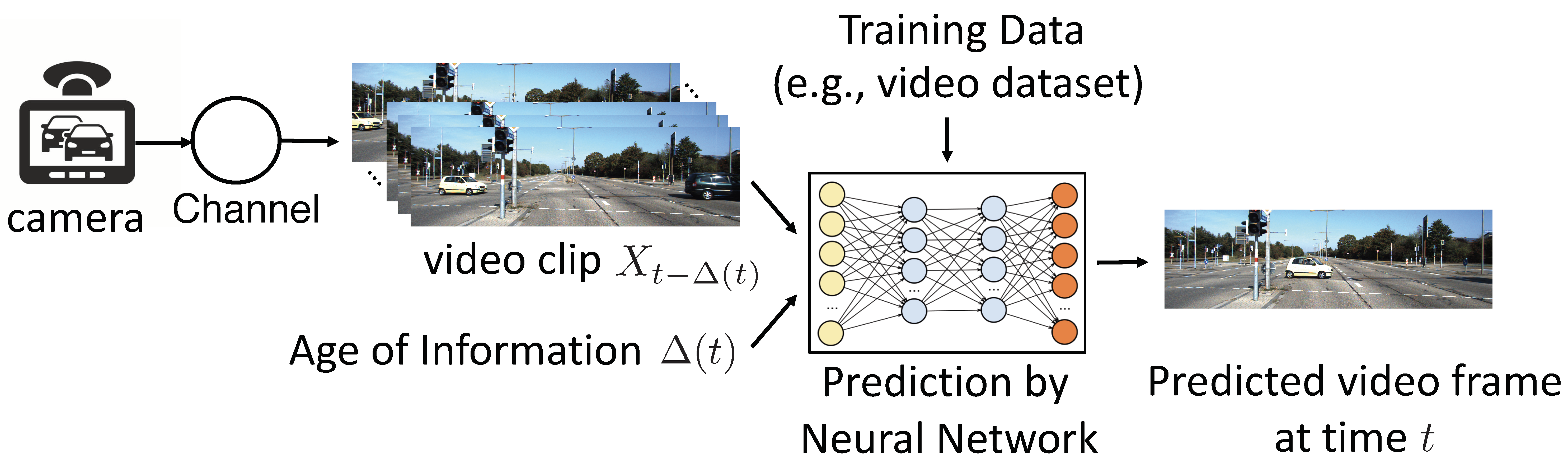
  (a) Video prediction Task

  

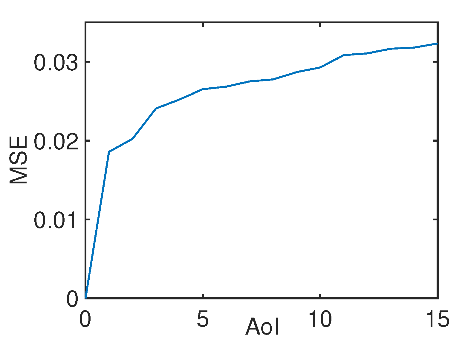
  (b) Training Error vs. AoI

  

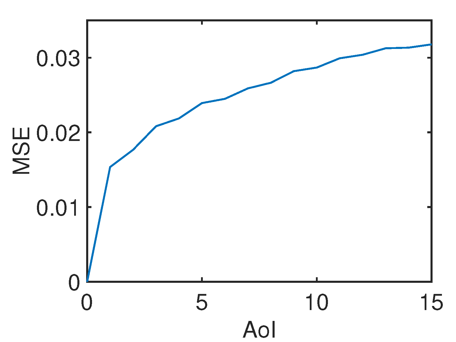
  (c) Inference Error vs. AoI

  Figure 1: Performance of supervised learning based video prediction. The experimental results in (b) and (c) are regenerated from [9]. The training and inference errors are non-decreasing functions of the AoI.

• We propose buffer management and transmission scheduling strategies to minimize the inference error. Because the inference error could be a non-monotonic AoI function, we introduce a novel “selection-from-buffer” model for feature transmissions, which is more general than the “generate-at-will” model used in many earlier studies, e.g., [7, 6, 10]. If the AoI function is non-decreasing, the “selection-from-buffer” model achieves same performance as the “generate-at-will” model; if the AoI function is non-monotonic, the “selection-from-buffer” model can potentially achieve better performance.

• In the single-source case, an optimal scheduling policy is devised to minimize the long-term average inference error. By exploiting a new connection with the Gittins index theory [11], the optimal scheduling policy is proven to be a threshold policy on the Gittins index (Theorems 4-5), where the threshold can be computed by using a low complexity algorithm like bisection search. This scheduling policy is more general than the scheduling policies proposed in [6, 7].

• In the multi-source case, a Whittle index scheduling policy is designed to reduce the weighted sum of the inference errors of the sources. By using the Gittins index obtained in the single-source case, a semi-analytical expression of the Whittle index is obtained (Theorems 6-7), which is more general than the Whittle index formula in [8, Equation (7)].

• The above scheduling results hold (i) for minimizing general AoI functions (monotonic or non-monotonic) and (ii) for general feature transmission time distributions. Data driven evaluations show that “selection-from-buffer” with optimal scheduler achieves up to $3$ times smaller inference error compared to “generate-at-will,” and $8$ times smaller inference error compared to periodic feature updating (see Fig. 8). Whittle index policy achieves up to $2$ times performance gain compared to maximum age first (MAF) policy (see Fig. 10).

I-A Related Works

In recent years, AoI has become a popular research topic [12]. Average AoI and average peak AoI are studied in many queueing systems [3, 7, 10]. As surveyed in [6], there exist a number of applications of non-linear AoI functions, such as auto-correlation function [5], estimation error [13, 14, 15], and Shannon’s mutual information and conditional entropy [6]. In existing studies on AoI, it was usually assumed that the observed data sequence is Markovian and the performance degradation caused by information aging was modeled as a monotonic AoI function. However, practical data sequence may not be Markovian [16, 6, 17]. In the present paper, theoretical results and experimental studies are provided to analyze the performance of real-time supervised learning for both Markovian and non-Markovian time-series data. In [18], impact of peak-AoI on the convergence speed of online training was analyzed. Unlike online training in [18], our work considers offline training and online inference.

Moreover, there are significant research efforts on the optimization of AoI functions by designing sampling and scheduling policies. Previous studies [7, 6, 14, 19, 8, 20] focused on non-decreasing AoI functions. Recently, a Whittle index based multi-source scheduling policy was derived in [21] to minimize Shannon’s conditional entropy that could be a non-monotonic function of the AoI. The Whittle index policy in [21] requires that (i) the state of each source evolves as binary Markov process, (ii) the AoI function is concave with respect to the belief state of the Markov process, and (iii) the packet transmission time is constant. The results in [6, 14, 7, 19, 8, 20, 21] are not appropriate for minimizing general (potentially non-monotonic) AoI functions, as considered in the present paper.

II Information-theoretic Measures for Real-time Supervised Learning

II-A Freshness-aware Learning Model

Consider the real-time supervised learning system illustrated in Fig. 1, where the goal is to predict a label $Y_{t}\in\mathcal{Y}$ (e.g., the location of the car in front) at each time $t$ based on a feature $X_{t-\Delta(t)}$ (e.g., a video clip) that was generated $\Delta(t)$ seconds ago. The feature, $X_{t-\Delta(t)}=(V_{t-\Delta(t)},\ldots,V_{t-\Delta(t)-u+1})$ is a time sequence with length $u$ (e.g., each video clip consisting of $u$ consecutive video frames). We consider a class of popular supervised learning algorithms called Empirical Risk Minimization (ERM) [22]. In freshness-aware ERM algorithms, a neural network is trained to construct an action $a=\phi(X_{t-\Delta(t)},\Delta(t))\in\mathcal{A}$ where $\phi:\mathcal{X}\times\mathcal{D}\mapsto\mathcal{A}$ is a function of feature $X_{t-\Delta(t)}\in\mathcal{X}$ and its AoI $\Delta(t)\in\mathcal{D}$. The performance of learning is measured by a loss function $L:\mathcal{Y}\times\mathcal{A}\mapsto\mathbb{R}$, where $L(y,a)$ is the incurred loss if action $a$ is chosen by the neural network when $Y_{t}=y$. We assume that $\mathcal{Y}$, $\mathcal{X}$, and $\mathcal{D}$ are discrete and finite sets. The loss function $L$ is determined by the targeted application of the system. For example, in neural network based estimation, the loss function is usually chosen as the square estimation error $L_{2}(\mathbf{y},\hat{\mathbf{y}})=\|\mathbf{y}-\hat{\mathbf{y}}\|^{2}$, where the action $a=\hat{y}$ is an estimate of $Y_{t}=y$. In softmax regression (i.e., neural network based maximum likelihood classification), the action $a=Q_{Y}$ is a distribution of $Y_{t}$ and the loss function $L_{\text{log}}(y,Q_{Y})=-\text{log}~{}Q_{Y}(y)$ is the negative log-likelihood of the label value $Y_{t}=y$. Therefore, the loss function $L$ characterizes the goal and purpose of a specific application.

II-B Offline Training Error

The real-time supervised learning system that we consider consists of two phases: offline training and online inference. In the offline training phase, the neural network is trained using a training dataset. Let $P_{\tilde{Y}_{0},\tilde{X}_{-\Theta},\Theta}$ denote the empirical distribution of the label $\tilde{Y}_{0}$, feature $\tilde{X}_{-\Theta}$, and AoI $\Theta$ in the training dataset, where the AoI $\Theta\geq 0$ of the feature $\tilde{X}_{-\Theta}$ is the time difference between $\tilde{Y}_{0}$ and $\tilde{X}_{-\Theta}$. In ERM algorithms, the training problem is formulated as

$$\mathrm{err}_{\mathrm{training}}=\min_{\phi\in\Lambda}\mathbb{E}_{Y,X,\Theta\sim P_{\tilde{Y}_{0},\tilde{X}_{-\Theta},\Theta}}[L(Y,\phi(X,\Theta))],$$ (1)

where $\Lambda$ is the set of functions that can be constructed by the neural network, and $\mathrm{err}_{\mathrm{training}}$ is the minimum training error. The optimal solution to (1) is denoted by $\phi^{*}_{P_{\tilde{Y}_{0},\tilde{X}_{-\Theta},\Theta}}$.

Let $\Phi=\{f:\mathcal{X}\times\mathcal{D}\mapsto\mathcal{A}\}$ be the set of all functions mapping from $\mathcal{X}\times\mathcal{D}$ to $\mathcal{A}$. Any action $\phi(x,\theta)$ constructed by the neural network belongs to $\Phi$, whereas the neural network cannot produce some functions in $\Phi$. Hence, $\Lambda\subset\Phi$. By relaxing the feasible set $\Lambda$ in (1) as $\Phi$, we obtain a lower bound of $\mathrm{err}_{\mathrm{training}}$, i.e.,

$$H_{L}(\tilde{Y}_{0}|\tilde{X}_{-\Theta},\Theta)=\min_{\phi\in\Phi}\mathbb{E}_{Y,X,\Theta\sim P_{\tilde{Y}_{0},\tilde{X}_{-\Theta},\Theta}}[L(Y,\phi(X,\Theta))],$$ (2)

where $H_{L}(\tilde{Y}_{0}|\tilde{X}_{-\Theta},\Theta)$ is a generalized conditional entropy of $\tilde{Y}_{0}$ given $(\tilde{X}_{-\Theta},\Theta)$ [23, 24, 25]. Compared to $\mathrm{err}_{\mathrm{training}}$, its information-theoretic lower bound $H_{L}(\tilde{Y}_{0}|\tilde{X}_{-\Theta},\Theta)$ is mathematically more convenient to analyze. The gap between $\mathrm{err}_{\mathrm{training}}$ and the lower bound $H_{L}(\tilde{Y}_{0}|\tilde{X}_{-\Theta},\Theta)$ was studied recently in [26], where the gap is small if the function spaces $\Lambda$ and $\Phi$ are close to each other, e.g., when the neural network is sufficiently wide and deep [22].

For notational convenience, we refer to $H_{L}(\tilde{Y}_{0}|\tilde{X}_{-\Theta},\Theta)$ as an L-conditional entropy, because it is associated with a loss function $L$. The $L$-entropy of a random variable $Y$ is defined as [23, 25]

$$H_{L}(Y)=\min_{a\in\mathcal{A}}\mathbb{E}_{Y\sim P_{Y}}[L(Y,a)].$$ (3)

Let $a_{P_{Y}}$ denote an optimal solution to (3), which is called a Bayes action [23]. The $L$-conditional entropy of $Y$ given $X=x$ is

$$H_{L}(Y|X=x)=\min_{a\in\mathcal{A}}\!\mathbb{E}_{Y\sim P_{Y|X=x}}[L(Y,a)].$$ (4)

Using (4), we can get the $L$-conditional entropy of $Y$ given $X$ [23, 25]

$$H_{L}(Y|X)=\sum_{x\in\mathcal{X}}P_{X}(x)H_{L}(Y|X=x).$$ (5)

Similar to (5), (2) can be decomposed as

$$H_{L}(\tilde{Y}_{0}|\tilde{X}_{-\Theta},\Theta)$$

$$= \sum_{\begin{subarray}{c}x\in\mathcal{X},\theta\in\mathcal{D}\end{subarray}}\!\!\!\!P_{\tilde{X}_{-\Theta},\Theta}(x,\theta)H_{L}(\tilde{Y}_{0}|\tilde{X}_{-\theta}=x,\Theta=\theta).\!\!\!$$ (6)

We assume that in the training dataset, the AoI $\Theta$ is independent of the label $\tilde{Y}_{0}$ and feature $\tilde{X}_{-\mu}$ for all $\mu\geq 0$. By this assumption and (II-B), one can get (see Appendix VIII-C for its proof)

$$\!\!H_{L}(\tilde{Y}_{0}|\tilde{X}_{-\Theta},\Theta)\!=\sum_{\theta\in\mathcal{D}}P_{\Theta}(\theta)~{}H_{L}(\tilde{Y}_{0}|\tilde{X}_{-\theta}).$$ (7)

The $L$-divergence $D_{L}(P_{Y}||P_{\tilde{Y}})$ of $P_{Y}$ from $P_{\tilde{Y}}$ can be expressed as [23, 25]

$$\!\!\!\!\!\!D_{L}(P_{Y}||P_{\tilde{Y}})\!=\!\mathbb{E}_{Y\sim P_{\tilde{Y}}}\left[L\left(Y,a_{P_{Y}}\right)\right]-\mathbb{E}_{Y\sim P_{\tilde{Y}}}\left[L\left(Y,a_{P_{\tilde{Y}}}\right)\right]\geq 0.$$ (8)

The $L$-mutual information $I_{L}(Y;X)$ is defined as [23, 25]

$$I_{L}(Y;X)= \mathbb{E}_{X\sim P_{X}}\left[D_{L}\left(P_{Y|X}||P_{Y}\right)\right]$$

$$= H_{L}(Y)-H_{L}(Y|X)\geq 0,$$ (9)

which measures the performance gain in predicting $Y$ by observing $X$. In general, $I_{L}(Y;X)$ $\neq$ $I_{L}(X;Y)$. The $L$-conditional mutual information $I_{L}(Y;X|Z)$ is given by

$$I_{L}(Y;X|Z)= \mathbb{E}_{X,Z\sim P_{X,Z}}\left[D_{L}\left(P_{Y|X,Z}||P_{Y|Z}\right)\right]$$

$$= H_{L}(Y|Z)-H_{L}(Y|X,Z).$$ (10)

The relationship among $L$-divergence, Bregman divergence [27], and $f$-divergence [28] is discussed in Appendix VIII-A. We note that any Bregman divergence is an $L$-divergence, and an $L$-divergence is a Bregman divergence only if $H_{L}(Y_{t})$ is continuously differentiable and strictly concave in $\mathcal{P}_{Y_{t}}$ [23]. Examples of loss function $L$, $L$-entropy, and $L$-cross entropy are provided in Appendix VIII-B.

II-C Online Inference Error

In the online inference phase, the neural predictor trained by (1) is used to predict the target in real-time. We assume that $\{(Y_{t},X_{t}),t\in\mathbb{Z}\}$ is a stationary process that is independent of the AoI process $\{\Delta(t),t\in\mathbb{Z}\}$. Using this assumption, the time-average expected inference error during the time slots $t=0,1,\ldots,T-1$ is given by

$$\mathrm{err}_{\mathrm{inference}}(T)=\frac{1}{T}\mathbb{E}\left[\sum_{t=0}^{T-1}p(\Delta(t))\right],$$ (11)

where

$$p(\delta)=\mathbb{E}_{Y,X\sim P_{Y_{t},X_{t-\delta}}}\left[L\left(Y,\phi^{*}_{P_{\tilde{Y}_{0},\tilde{X}_{-\Theta},\Theta}}(X,\delta)\right)\right],$$ (12)

$p(\Delta(t))$ is the expected inference error in time slot $t$, and $\Delta(t)$ is the inference AoI at time $t$, i.e., the time difference between label $Y_{t}$ and feature $X_{t-\Delta(t)}$. The proof of (11) is provided in Appendix VIII-D.

Let us define $L$-cross entropy between $Y$ and $\tilde{Y}$ as

$$H_{L}(Y;\tilde{Y})=\mathbb{E}_{Y\sim P_{Y}}\left[L\left(Y,a_{P_{\tilde{Y}}}\right)\right],$$ (13)

and $L$-conditional cross entropy between $Y$ and $\tilde{Y}$ given $X$ as

$$H_{L}(Y;\tilde{Y}|X)=\sum_{x\in\mathcal{X}}P_{X}(x)\mathbb{E}_{Y\sim P_{Y|X=x}}\left[L\left(Y,a_{P_{\tilde{Y}|\tilde{X}=x}}\right)\right],$$ (14)

where $a_{P_{\tilde{Y}}}$ and $a_{P_{\tilde{Y}|\tilde{X}=x}}$ are the Bayes actions associated with $P_{\tilde{Y}}$ and $P_{\tilde{Y}|\tilde{X}=x}$, respectively. If the neural predictor in (12) is replaced by the Bayes action $a_{\tilde{Y}_{0}|\tilde{X}_{-\delta}=x}$, i.e., the optimal solution to (2), then $p(\delta)$ becomes an $L$-conditional cross entropy

$$H_{L}(Y_{t};\tilde{Y}_{0}|X_{t-\delta})\!\!$$

$$= \!\!\!\sum_{x\in\mathcal{X}}\!\!P_{X_{t-\delta}}(x)\mathbb{E}_{Y\sim P_{Y_{t}|X_{t-\delta}=x}}\!\!\left[L\left(Y,a_{\tilde{Y}_{0}|\tilde{X}_{-\delta}=x}\right)\right]\!.\!\!\!\!$$ (15)

If the function spaces $\Lambda$ and $\Phi$ are close to each other, the difference between $p(\delta)$ and $H_{L}(Y_{t};\tilde{Y}_{0}|X_{t-\delta})$ is small.

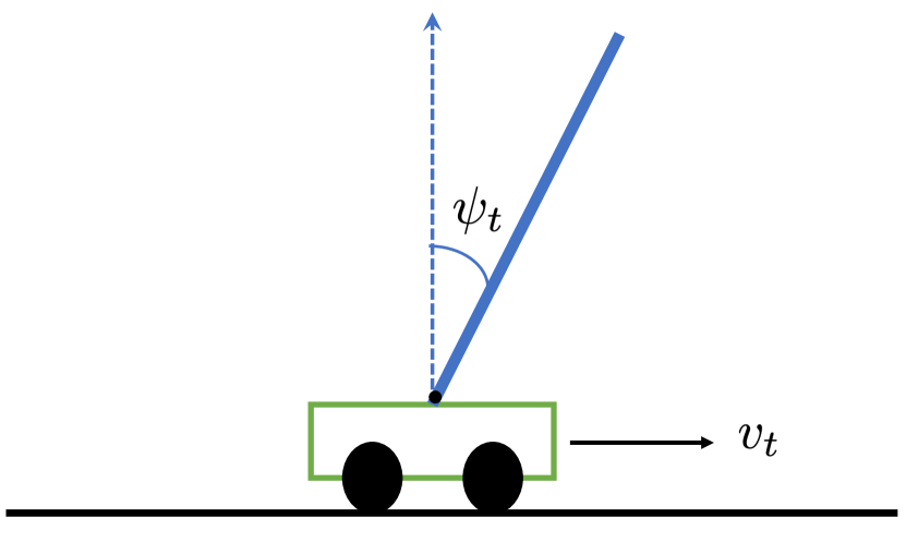
(a) OpenAI Cart Pole Task

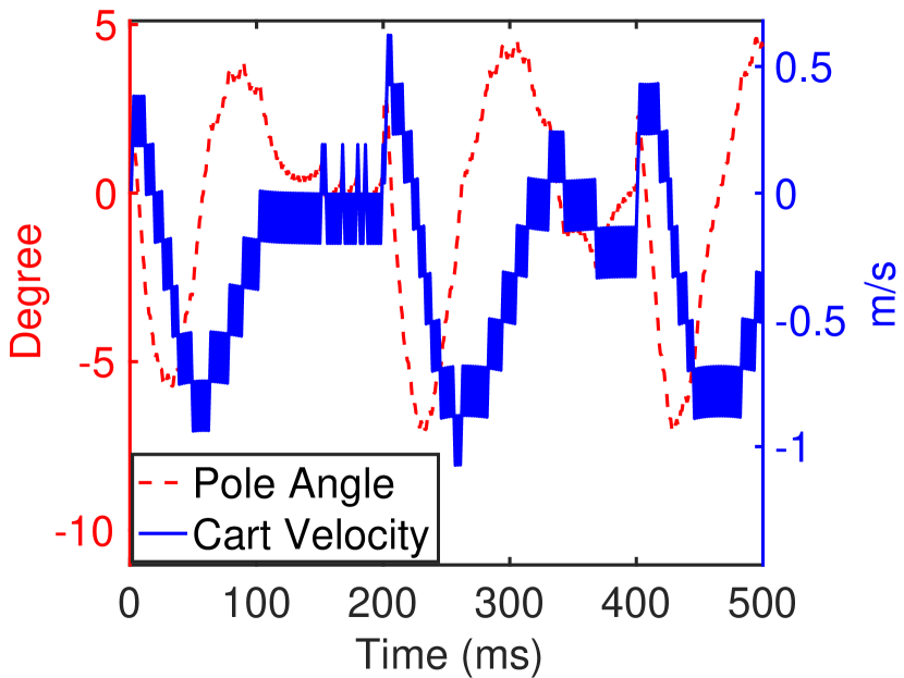
(b) Data Traces

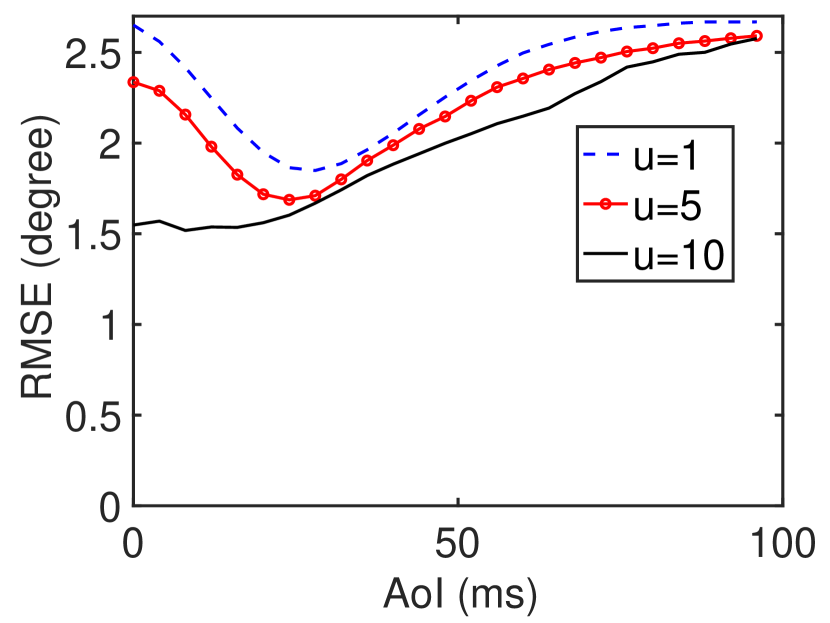
(c) Training Error vs. AoI

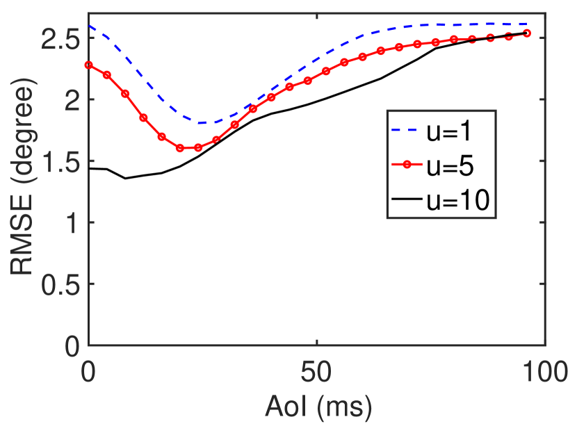
(d) Inference Error vs. AoI

Figure 2: Performance of actuator state prediction under mechanical response delay. In the OpenAI CartPole-v1 task [29], the pole angle $\psi_{t}$ is predicted by using the cart velocity $v_{t-\delta}$ with an AoI $\delta$. Because of the mechanical response delay between cart velocity and pole angle, the training error and inference error are non-monotonic in the AoI.

III Interpretation of Freshness in Real-time Supervised Learning

In this section, we study how the training AoI $\Theta$ and the inference AoI $\Delta(t)$ affect the performance of real-time supervised learning.

III-A Training Error vs. Training AoI

We first consider the case of deterministic training AoI $\Theta=\theta$. Given $\Theta=\theta$, $H_{L}(\tilde{Y}_{0}|\tilde{X}_{-\Theta},\Theta)$ in (7) becomes simply $H_{L}(\tilde{Y}_{0}|\tilde{X}_{-\theta})$, which is a function of $\theta$. One may expect that the training error would grow with the AoI $\theta$. If $\tilde{Y}_{0}\leftrightarrow\tilde{X}_{-\mu}\leftrightarrow\tilde{X}_{-\mu-\nu}$ is a Markov chain for all $\mu,\nu\geq 0$, by the data processing inequality for $L$-conditional entropy [24, Lemma 12.1], one can show that $H_{L}(\tilde{Y}_{0}|\tilde{X}_{-\theta})$ is a non-decreasing function of $\theta$. Nevertheless, the experimental results in Figs. 1-4 and [4] show that the training error is a growing function of the training AoI $\theta$ in some applications (e.g., video prediction), whereas it is a non-monotonic function of $\theta$ in other applications (e.g., temperature prediction and actuator state prediction with delay). As we will explain below, a fundamental reason behind these phenomena is that practical time-series data could be either Markovian or non-Markovian. For non-Markovian $(\tilde{Y}_{0},\tilde{X}_{-\mu},\tilde{X}_{-\mu-\nu})$, $H_{L}(\tilde{Y}_{0}|\tilde{X}_{-\theta})$ is not necessarily monotonic in $\theta$.

Next, we develop an $\epsilon$-data processing inequality to analyze information freshness for both Markovian and non-Markovian time-series data. To that end, the following relaxation of the standard Markov chain model is needed, which is motivated by [30]:

Definition 1 ($\epsilon$-Markov Chain).

Given $\epsilon\geq 0$, a sequence of three random variables $Z,X,$ and $Y$ is said to be an $\epsilon$-Markov chain, denoted as $Z\overset{\epsilon}{\rightarrow}X\overset{\epsilon}{\rightarrow}Y$, if

$$I_{\chi^{2}}(Y;Z|X)=\mathbb{E}_{X,Z\sim P_{X,Z}}\left[D_{\chi^{2}}\left(P_{Y|X,Z}||P_{Y|X}\right)\right]\leq\epsilon^{2},$$ (16)

where

$$D_{\chi^{2}}(P_{Y}||Q_{Y})=\sum_{y\in\mathcal{Y}}\frac{(P_{Y}(y)-Q_{Y}(y))^{2}}{Q_{Y}(y)}$$ (17)

is Neyman’s $\chi^{2}$-divergence and $I_{\chi^{2}}(Y;Z|X)$ is $\chi^{2}$-conditional mutual information.

A Markov chain is an $\epsilon$-Markov chain with $\epsilon=0$. If $Z\rightarrow X\rightarrow Y$ is a Markov chain, then $Y\rightarrow X\rightarrow Z$ is also a Markov chain [32, p. 34]. A similar property holds for the $\epsilon$-Markov chain.

Lemma 1.

If $Z\overset{\epsilon}{\rightarrow}X\overset{\epsilon}{\rightarrow}Y$, then $Y\overset{\epsilon}{\rightarrow}X\overset{\epsilon}{\rightarrow}Z$.

Proof.

See Appendix VIII-E. ∎

By Lemma 1, the $\epsilon$-Markov chain can be denoted as $Y\overset{\epsilon}{\leftrightarrow}X\overset{\epsilon}{\leftrightarrow}Z$. In the following lemma, we provide a relaxation of the data processing inequality for $\epsilon$-Markov chain, which is called an $\epsilon$-data processing inequality.

Lemma 2 ($\epsilon$-data processing inequality).

If $Y\overset{\epsilon}{\leftrightarrow}X\overset{\epsilon}{\leftrightarrow}Z$ is an $\epsilon$-Markov chain, then

$$H_{L}(Y|X)\leq H_{L}(Y|Z)+O(\epsilon).$$ (18)

If, in addition, $H_{L}(Y)$ is twice differentiable in $P_{Y}$, then

$$H_{L}(Y|X)\leq H_{L}(Y|Z)+O(\epsilon^{2}).$$ (19)

Proof.

Lemma 2 is proven by using a local information geometric analysis; see Appendix VIII-F for the details. ∎

Lemma 2(b) was mentioned in [4] without proof. Lemma 2(a) is new to the best of our knowledge. Now, we are ready to characterize how $H(\tilde{Y}_{0}|\tilde{X}_{-\theta})$ varies with the AoI $\theta$.

Theorem 1.

The $L$-conditional entropy

$$H_{L}(\tilde{Y}_{0}|\tilde{X}_{-\theta})=g_{1}(\theta)-g_{2}(\theta)$$ (20)

is a function of $\theta$, where $g_{1}(\theta)$ and $g_{2}(\theta)$ are two non-decreasing functions of $\theta$, given by

$$\!\!g_{1}(\theta)= H_{L}(\tilde{Y}_{0}|\tilde{X}_{0})+\sum_{k=0}^{\theta-1}~{}I_{L}(\tilde{Y}_{0};\tilde{X}_{-k}|\tilde{X}_{-k-1}),~{}$$

$$g_{2}(\theta)= \sum_{k=0}^{\theta-1}I_{L}(\tilde{Y}_{0};\tilde{X}_{-k-1}|\tilde{X}_{-k}).\!\!\!$$ (21)

If $\tilde{Y}_{0}\overset{\epsilon}{\leftrightarrow}\tilde{X}_{-\mu}\overset{\epsilon}{\leftrightarrow}\tilde{X}_{-\mu-\nu}$ is an $\epsilon$-Markov chain for every $\mu,\nu\geq 0$, then $g_{2}(\theta)=O(\epsilon)$ and

$$H_{L}(\tilde{Y}_{0}|\tilde{X}_{-\theta})=g_{1}(\theta)+O(\epsilon).$$ (22)

Proof.

See Appendix VIII-G. ∎

According to Theorem 1, the monotonicity of $H_{L}(\tilde{Y}_{0}|\tilde{X}_{-\theta})$ in $\theta$ is characterized by the parameter $\epsilon\geq 0$ in the $\epsilon$-Markov chain model. If $\epsilon$ is small, then $\tilde{Y}_{0}\overset{\epsilon}{\leftrightarrow}\tilde{X}_{-\mu}\overset{\epsilon}{\leftrightarrow}\tilde{X}_{-\mu-\nu}$ is close to a Markov chain, and $H_{L}(\tilde{Y}_{0}|\tilde{X}_{-\theta})$ is nearly non-decreasing in $\theta$. If $\epsilon$ is large, then $\tilde{Y}_{0}\overset{\epsilon}{\leftrightarrow}\tilde{X}_{-\mu}\overset{\epsilon}{\leftrightarrow}\tilde{X}_{-\mu-\nu}$ is far from a Markov chain, and $H_{L}(\tilde{Y}_{0}|\tilde{X}_{-\theta})$ could be non-monotonic in $\theta$. Theorem 1 can be readily extended to random AoI $\Theta$ by using stochastic orders [33].

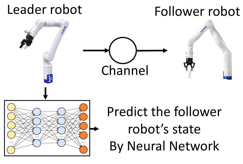
(a) Prediction of Follower Robot

(b) Training Error vs. AoI

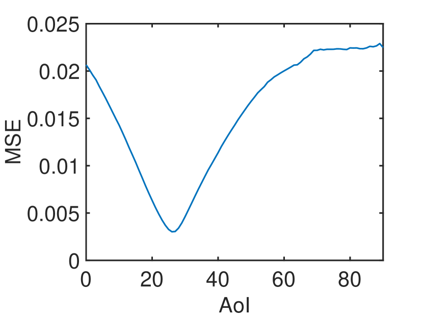
(c) Inference Error vs. AoI

Figure 3: Robot state prediction in a leader-follower robotic system. The leader robot uses a neural network to predict the follower robot’s state. The training and inference errors decrease in the AoI $\leq 25$ and increase when AoI $\geq 25$.

Definition 2 (Univariate Stochastic Ordering).

[33] A random variable $X$ is said to be stochastically smaller than another random variable $Z$, denoted as $X\leq_{st}Z$, if

$$P(X>x)\leq P(Z>x),\ \ \forall x\in\mathbb{R}.$$ (23)

Theorem 2.

If $\tilde{Y}_{0}\overset{\epsilon}{\leftrightarrow}\tilde{X}_{-\mu}\overset{\epsilon}{\leftrightarrow}\tilde{X}_{-\mu-\nu}$ is an $\epsilon$-Markov chain for all $\mu,\nu\geq 0$, and the training AoIs in two experiments $1$ and $2$ satisfy $\Theta_{1}\leq_{st}\Theta_{2}$, then

$$H_{L}(\tilde{Y}_{0}|\tilde{X}_{-\Theta_{1}},\Theta_{1})\leq H_{L}(\tilde{Y}_{0}|\tilde{X}_{-\Theta_{2}},\Theta_{2})+O(\epsilon).$$ (24)

Proof.

See Appendix VIII-H. ∎

According to Theorem 2, if $\Theta_{1}$ is stochastically smaller than $\Theta_{2}$, then the training error in Experiment 1 is approximately smaller than that in Experiment 2. If, in addition to the conditions in Theorems 3.4 and 3.6, $H_{L}(\tilde{Y}_{0})$ is twice differentiable in $P_{\tilde{Y}_{0}}$, then the last term $O(\epsilon)$ in (22) and (24) becomes $O(\epsilon^{2})$.

III-B Inference Error vs. Inference AoI

According to (4), (5), and (14), $H_{L}(Y_{t};\tilde{Y}_{0}|X_{t-\delta})$ is lower bounded by $H_{L}(Y_{t}|X_{t-\delta})$. In addition, $H_{L}(Y_{t};\tilde{Y}_{0}|X_{t-\delta})$ is close to its lower bound $H_{L}(Y_{t}|X_{t-\delta})$, if the conditional distributions $P_{Y_{t}|X_{t-\delta}}$ and $P_{\tilde{Y}_{0}|\tilde{X}_{-\delta}}$ are close to each other, as shown by the following lemma.

Lemma 3.

If for all $x\in\mathcal{X}$

$$D_{\chi^{2}}\left(P_{Y_{t}|X_{t-\delta}=x}||P_{\tilde{Y}_{0}|\tilde{X}_{-\delta}=x}\right)\!\!\leq\beta^{2},$$ (25)

then

$$H_{L}(Y_{t};\tilde{Y}_{0}|X_{-\delta})= H_{L}(Y_{t}|X_{t-\delta})+O(\beta).$$ (26)

Proof.

See Appendix VIII-I. ∎

If (25) is replaced by the condition

$$\sum_{x\in\mathcal{X}}P_{X_{t-\delta}}(x)~{}~{}D_{\chi^{2}}\left(P_{Y_{t}|X_{t-\delta}=x}||P_{\tilde{Y}_{0}|\tilde{X}_{-\delta}=x}\right)\!\!~{}\leq\beta^{2},$$ (27)

then Lemma 3 still holds. By combining Theorem 1 and Lemma 3, the monotonicity of $H_{L}(Y_{t};\tilde{Y}_{0}|X_{t-\delta})$ versus $\delta$ is characterized in the next theorem.

Theorem 3.

The following assertions are true:

• If $\{(Y_{t},X_{t}),t\in\mathbb{Z}\}$ is a stationary process, then $H_{L}(Y_{t};\tilde{Y}_{0}|X_{t-\delta})$ is a function of the inference AoI $\delta$.

• If, in addition, $Y_{t}\overset{\epsilon}{\leftrightarrow}X_{t-\mu}\overset{\epsilon}{\leftrightarrow}X_{t-\mu-\nu}$ is an $\epsilon$-Markov chain for all $\mu,\nu\geq 0$ and (25) holds for all $x\in\mathcal{X}$ and $\delta\in\mathcal{D}$, then for all $0\leq\delta_{1}\leq\delta_{2}$

  $$\!\!H_{L}(Y_{t};\tilde{Y}_{0}|X_{t-\delta_{1}})\leq H_{L}(Y_{t};\tilde{Y}_{0}|X_{t-\delta_{2}})+O\big{(}\max\{\epsilon,\beta\}\big{)}.$$ (28)

Proof.

See Appendix VIII-J. ∎

According to Theorem 3, $H_{L}(Y_{t};\tilde{Y}_{0}|X_{t-\delta})$ is a function of the inference AoI $\delta$. If $\epsilon$ and $\beta$ are close to zero, $H_{L}(Y_{t};\tilde{Y}_{0}|X_{t-\delta})$ is nearly a non-decreasing function of $\delta$; otherwise, $H_{L}(Y_{t};\tilde{Y}_{0}|X_{t-\delta})$ can be far from a monotonic function of $\delta$.

The $\epsilon$-Markov chain model that we propose can be viewed as a measure of conditional dependence. Different from earlier studies on conditional dependence measures [34, 35, 36, 37], we use a local information geometric approach to characterize how the non-Markov property of the data affects the relationship between AoI and the performance of real-time forecasting.

III-C Interpretation of Experimental Results

We conduct several experiments to study how the training and inference errors of real-time supervised learning vary with the AoI. The code of these experiments is provided in an open-source Github repository.

Fig. 1 illustrates the experimental results of supervised learning based video prediction, which are regenerated from [9]. In this experiment, the video frame $V_{t}$ at time $t$ is predicted based on a feature $X_{t-\delta}=(V_{t-\delta},V_{t-\delta-1})$ that is composed of two consecutive video frames, where $\Delta(t)=\delta$ is the AoI. A pre-trained neural network model called “SAVP” [9] is used to evaluate on $256$ samples of “BAIR” dataset [38], which contains video frames of a randomly moving robotic arm. The pre-trained neural network model can be downloaded from the Github repository of [9]. One can observe from Fig. 1(b)-(c) that the training and inference errors are non-decreasing functions of the AoI, because the video clips $V_{t}$ are approximately a Markov chain.

Fig. 2 plots the performance of actuator state prediction under mechanical response delay. We consider the OpenAI CartPole-v1 task [29], where a DQN reinforcement learning algorithm [39] is used to control the force on a cart and keep the pole attached to the cart from falling over. By simulating $10^{4}$ episodes of the OpenAI CartPole-v1 environment, a time-series dataset is collected that contains the pole angle $\psi_{t}$ and the velocity $V_{t}$ of the cart. The pole angle $\psi_{t}$ at time $t$ is predicted based on a feature $X_{t-\delta}=(V_{t-\delta},\ldots,V_{t-\delta-u+1})$, i.e., a vector of cart velocity with length $u$, where $V_{t}$ is the cart velocity at time $t$ and $\Delta(t)=\delta$ is the AoI. The predictor in this experiment is an LSTM neural network that consists of one input layer, one hidden layer with 64 LSTM cells, and a fully connected output layer. First $72\%$ of the dataset is used for training and the rest of the dataset is used for inference. From the data trace in Fig. 2(b), one can observe a response (or reaction) delay of $25$-$30$ ms between cart velocity and pole angle. Such response delay exists broadly in mechanical, circuit, biological, economic, and physical systems that are modeled by differential equations. Due to the response delay, $\psi_{t}$ is strongly correlated with $V_{t-25}$, but quite different from $V_{t}$. Hence, $(\psi_{t},V_{t},V_{t}-25)$ is far from a Markov chain. This agrees with Fig. 2(c)-(d), where the training error and inference error are non-monotonic in the AoI for $u=1$.

According to Shannon’s interpretation of Markov sources in his seminal work [40], $(\psi_{t},X_{t-\mu},X_{t-\mu-\nu})$ becomes closer to a Markov chain, as the size $u$ of feature vector $X_{t-\delta}=(V_{t-\delta},\ldots,$ $V_{t-\delta-u+1})$ increases. In fact, $(\psi_{t},X_{t-\mu},X_{t-\mu-\nu})$ is precisely a Markov chain if $u=\infty$. One can observe from Fig. 2(c)-(d) that, as $u$ grows, the training and inference errors get close to non-decreasing functions of the AoI. This is because $(\psi_{t},X_{t-\mu},X_{t-\mu-\nu})$ tends to be Markovian as $u$ increases, i.e., the parameter $\epsilon$ of the $\epsilon$-Markov chain $\psi_{t}\overset{\epsilon}{\leftrightarrow}X_{t-\mu}\overset{\epsilon}{\leftrightarrow}X_{t-\mu-\nu}$ reduces to zero as $u$ grows. We note that one disadvantage of large feature size $u$ is that it increases the channel capacity needed for transmitting the features.

Fig. 3 depicts the performance of robot state prediction in a leader-follower robotic system. As illustrated in a Youtube video , the leader robot sends its state (joint angles) $X_{t}$ to the follower robot through a channel. One packet for updating the leader robot’s state is sent periodically to the follower robot every $20$ time-slots. The transmission time of each updating packet is $20$ time-slots. The follower robot moves towards the leader’s most recent state and locally controls its robotic fingers to grab an object. We constructed a robot simulation environment using the Robotics System Toolbox in MATLAB. In each episode, a can is randomly generated on a table in front of the follower robot. The leader robot observes the position of the can and illustrates to the follower robot how to grab the can and place it on another table, without colliding with other objects in the environment. The rapidly-exploring random tree (RRT) algorithm is used to control the leader robot. Collision avoidance algorithm and trajectory generation algorithm are used for local control of the follower robot. The leader robot uses a neural network to predict the follower robot’s state $Y_{t}$. The neural network consists of one input layer, one hidden layer with $256$ ReLU activation nodes, and one fully connected (dense) output layer. The dataset contains the leader and follower robots’ states in 300 episodes of continue operation. The first $80\%$ of the dataset is used for the training and the other $20\%$ of the dataset is used for the inference. In Fig. 3, the training and the inference error decreases in AoI, when AoI $\leq 25$ and increases in AoI when AoI $\geq 25$. In this case, even a fresh feature with AoI=0 is not good for prediction. In this experiment, $(Y_{t},X_{t-\mu},X_{t-\mu-\nu})$ is not a Markov chain for all $\mu,\nu\geq 0$. Hence, the training and the inference error are not non-decreasing functions of AoI.

To facilitate understanding the experimental results in Fig. 3, we provide a toy example to interpret it: Let $X_{t}$ be a Markov chain and $Y_{t}=f(X_{t-d})$. One can view $X_{t}$ as the input of a causal system with delay $d\geq 0$, and $Y_{t}$ as the system output. Because $Y_{t}=f(X_{t-d})$, a stale system input $X_{t-d}$ at time $t-d$ is informative for inferring the current output $Y_{t}$ at time $t$. If the training and inference datasets have similar empirical distributions, by using Lemma 7 from Appendix VIII-Q, we get $H_{L}(\tilde{Y}_{0}|\tilde{X}_{\delta})$ and $H_{L}(Y_{t};\tilde{Y}_{0}|X_{t-\delta})$ decrease with $\delta$ when $0\leq\delta\leq d$ and increase with $\delta$ when $\delta\geq d$, which is similar to Fig. 3. Moreover, $H_{L}(\tilde{Y}_{0}|\tilde{X}_{d})$ is close to zero if the function space $\Lambda$ is sufficiently large. It is equal to zero if $\Lambda=\Phi$. The leader-follower robotic system in Fig. 3 can be viewed as a causal system, where the system input is the leader robot’s state, and the system output is the follower robot’s state. Non-monotonicity occurs in Fig. 3 because the input of a causal system is used to predict the system output in this experiment, which is similar to the toy example. However, the relationship between the system input and output in Fig. 3 is more complicated than the toy example, due to the control algorithms used by the follower robot.

In Fig. 4, we plot the performance of temperature prediction. In this experiment, the temperature $Y_{t}$ at time $t$ is predicted based on a feature $X_{t-\delta}=\{s_{t-\delta},\ldots,s_{t-\delta-u+1}\}$, where $s_{t}$ is a $7$-dimensional vector consisting of the temperature, pressure, saturation vapor pressure, vapor pressure deficit, specific humidity, airtight, and wind speed at time $t$. Similar to [41], we have used an LSTM neural network and Jena climate dataset recorded by Max Planck Institute for Biogeochemistry. In this experiment, time unit of the sequence is $1$ hour. Due to the long-range dependence of weather data, if $u=1,6,$ or $12$, $(Y_{t},X_{t-\mu},X_{t-\mu-\nu})$ is not a Markov chain. If $u=24$, then $Y_{t}\leftrightarrow X_{t-\mu}\leftrightarrow X_{t-\mu-\nu}$ is close to a Markov chain. Hence, when $u=1,6,$ or $12$, the training error and the inference error are non-monotonic in AoI and when $u=24$, the training error and the inference error are close to a non-decreasing function of AoI.

Fig. 5 illustrates the performance of channel state information (CSI) prediction. The CSI $h_{t}$ at time $t$ is predicted based on a feature $X_{t-\delta}=\{h_{t-\delta},\ldots,h_{t-\delta-u+1}\}$. The dataset for CSI is generated by using Jakes model [42]. Due to long-range dependence of CSI, the training error and the inference error are non-monotonic in AoI. However, they become non-decreasing functions of AoI as $u$ grows. The phenomenon of long-range dependence is also observed in solar power prediction [4].

IV Single-source Scheduling for Inference Error Minimization

As shown in Section III, the inference error is a function of the AoI $\Delta(t)$, whereas the function is not necessarily monotonic. To reduce the inference error, we devise a new scheduling algorithm that can minimize general functions of the AoI, no matter whether the function is monotonic or not.

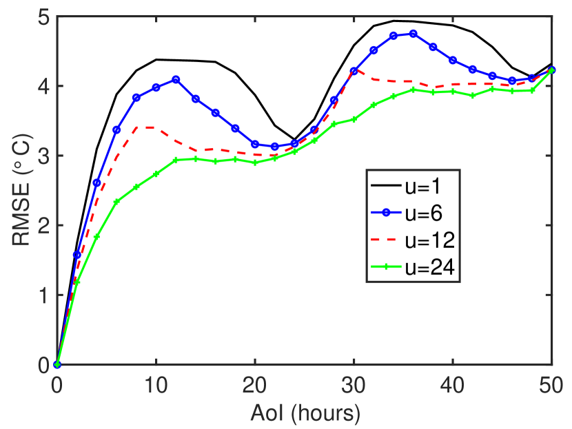
(a) Training Error vs. AoI

(b) Inference Error vs. AoI

Figure 4: Performance of temperature Prediction. The training error and inference error are non-monotonic in AoI. As $u$ increases, the errors tend closer to non-decreasing functions of the AoI.

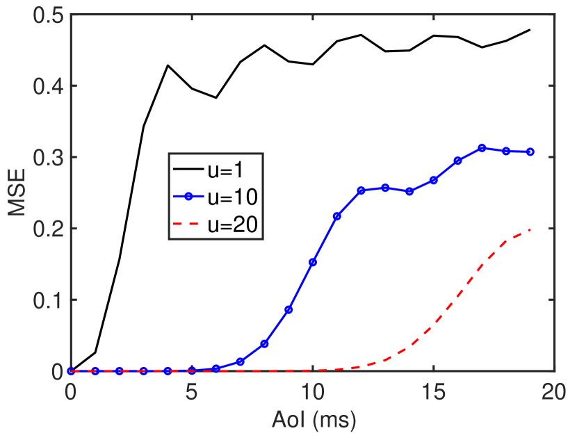
(a) Training Error vs. AoI

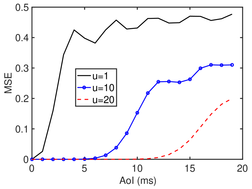
(b) Inference Error vs. AoI

Figure 5: Performance of channel state information (CSI) prediction. The training error and inference error are non-monotonic in AoI. As $u$ increases, the errors tend closer to non-decreasing functions of the AoI.

IV-A System Model

We consider the networked supervised learning system in Fig. 6, where a source progressively sends features through a channel to a receiver. The channel is modeled as a non-preemptive server with i.i.d. service times. At any time $t$, the receiver uses the latest received feature to predict the current label $Y_{t}$. To minimize the inference error, we propose a new “selection-from-buffer” model for feature transmissions, which is more general than the “generate-at-will” model [10]. Specifically, at the beginning of time slot $t$, the source generates a fresh feature $X_{t}$ and appends it to a buffer that stores the $B$ most recent features $(X_{t},X_{t-1},\ldots,X_{t-B+1})$; meanwhile, the oldest feature $X_{t-B}$ is removed from the buffer. The transmitter can pick any feature from the buffer and submit it to the channel when the channel is idle. A transmission scheduler determines (i) when to submit features to the channel and (ii) which feature in the buffer to submit. When $B=1$, the “selection-from-buffer” model reduces to the “generate-at-will” model.

We assume that the system starts to operate in time slot $t=0$ with $B$ features $(X_{0},X_{-1},\ldots,X_{-B+1})$ in the buffer. Hence, the feature buffer is full at all time $t\geq 0$. The $i$-th feature sent over the channel is generated in time slot $G_{i}$, is submitted to the channel in time slot $S_{i}$, is delivered and available for inference in time slot $D_{i}=S_{i}+T_{i}$, where $T_{i}\geq 1$ is the feature transmission time, $G_{i}\leq S_{i}<D_{i}$, and $D_{i}\leq S_{i+1}<D_{i+1}$. The feature transmission times $T_{i}$ could be random due to time-varying channel conditions, congestion, random packet sizes, etc. We assume that the $T_{i}$’s are i.i.d. with a finite mean $1\leq\mathbb{E}[T_{i}]<\infty$. In time slot $t=S_{i}$, the $(b_{i}+1)$-th freshest feature in the buffer is submitted to the channel, where $b_{i}\in\{0,1,\ldots,B-1\}$. Hence, the submitted feature is $X_{S_{i}-b_{i}}$ that was generated at time $G_{i}=S_{i}-b_{i}$. Once a feature is delivered, an acknowledgment (ACK) is fed back to the transmitter in the same time slot. Thus, the idle/busy state of the channel is known at the transmitter.

IV-B Scheduling Problem

Let $U(t)=\max_{i}\{G_{i}:D_{i}\leq t\}$ be the generation time of the latest received feature in time slot $t$. The age of information (AoI) at time $t$ is given by [3]

$$\Delta(t)=t-U(t)=t-\max_{i}\{G_{i}:D_{i}\leq t\}.$$ (29)

Because $D_{i}<D_{i+1}$, $\Delta(t)$ can be also written as

$$\Delta(t)=t-G_{i}=t-S_{i}+b_{i},~{}~{}\mathrm{if}~{}~{}D_{i}\leq t<D_{i+1}.$$ (30)

The initial state of the system is assumed to be $S_{0}=0,D_{0}=T_{0}$, and $\Delta(0)$ is a finite constant.

A scheduling policy is denoted by a 2-tuple $(f,g)$, where $g=(S_{1},S_{2},\ldots)$ determines when to submit the features and  $f=(b_{1},b_{2},$ $\ldots)$ specifies which feature in the buffer to submit. We consider the class of causal scheduling policies in which each decision is made by using the current and historical information available at the transmitter. Let $\Pi$ denote the set of all causal scheduling policies. We assume that the scheduler has access to the distribution of $\{(Y_{t},X_{t}),t\in\mathbb{Z}\}$ but not its realization, and the $T_{i}$’s are not affected by the adopted scheduling policy.

Our goal is to find an optimal scheduling policy that minimizes the time-average expected inference error among all causal scheduling policies in $\Pi$:

$$\bar{p}_{opt}=\inf_{(f,g)\in\Pi}\limsup_{T\rightarrow\infty}\frac{1}{T}\mathbb{E}_{(f,g)}\left[\sum_{t=0}^{T-1}p(\Delta(t))\right].$$ (31)

where $p(\Delta(t))$ is the inference error at time slot $t$, defined in (12), and $\bar{p}_{opt}$ is the optimum value of (31). Because $p(\cdot)$ is not necessarily a non-decreasing function, (31) is more challenging than the scheduling problems in [6, 7].

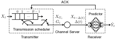
Figure 6: A networked real-time supervised learning system. At each time slot $t$, the transmitter generates a feature $X_{t}$ and keeps it in a buffer that stores $B$ most recent features $(X_{t},X_{t-1},\ldots,X_{t-B+1}$). The scheduler decides when to submit features to the channel and which feature in the buffer to submit.

IV-C Optimal Single-source Scheduling

We solve (31) in two steps: (i) Given a fixed feature selection policy $f_{b}=(b,b,\ldots)$ with $b_{i}=b$ for all $i$, find the optimal feature submission times $g=(S_{1},S_{2},\ldots)$ that solves

$$\bar{p}_{b}=\inf_{(f_{b},g)\in\Pi}\limsup_{T\rightarrow\infty}\frac{1}{T}\mathbb{E}_{(f_{b},g)}\left[\sum_{t=0}^{T-1}p(\Delta(t))\right],$$ (32)

(ii) Use the solution to (32) to describe an optimal solution to (31).

It turns out that optimal solution to (32) can be obtained by using the Gittins index of the following AoI bandit process with a random termination delay $T_{1}$: A bandit process $\Delta(t)$ is controlled by a decision-maker that chooses between two actions Continue and Stop in each time slot. If the bandit process is not terminated in time slot $t$, its state evolves according to

$$\Delta(t)=\Delta(t-1)+1,$$ (33)

and a reward $[r-p(\Delta(t))]$ is collected, where $p(\cdot)$ is defined in (12) and $r$ is a constant reward. If the Continue action is selected, the bandit process continues to evolve. If the Stop action is selected, the bandit process will terminate after a random delay $T_{1}$ and no more action is taken. Once the bandit process terminates, its state and reward remain zero. The total profit of the bandit process starting from time $t$ is maximized by solving the following optimal stopping problem:

$$\sup_{\nu\in\mathfrak{M}}\mathbb{E}\left[\sum_{k=0}^{\nu+T_{1}-1}[r-p(\Delta(t+k))]\bigg{|}\Delta(t)=\delta\right],$$ (34)

where $\nu\geq 0$ is a history-dependent stopping time and $\mathfrak{M}$ is the set of all stopping times of the bandit process $\{\Delta(t+k),k=0,1,\ldots\}$. Following the derivation of the Gittins index in [11, Chapter 2.5], the decision-maker should choose the Stop action at time

$$\min_{t\in\mathbb{Z}}\{t\geq 0:\gamma(\Delta(t))\geq r\},$$ (35)

where

$$\gamma(\delta)\!=\inf_{\nu\in\mathfrak{M},\nu\neq 0}\frac{\mathbb{E}\left[\sum_{k=0}^{\nu-1}p(\Delta(t+k+T_{1}))~{}\bigg{|}~{}\Delta(t)=\delta\right]}{\mathbb{E}[\nu~{}|~{}\Delta(t)=\delta]}$$ (36)

is the Gittins index, i.e., the value of reward $r$ for which the Continue and Stop actions are equally profitable at state $\Delta(t)=\delta$. As shown in Appendix VIII-K, (36) can be simplified as

$$\gamma(\delta)=\inf_{\tau\in\{1,2,\ldots\}}\frac{1}{\tau}\sum_{k=0}^{\tau-1}\mathbb{E}\left[p(\delta+k+T_{1})\right],$$ (37)

where $\tau$ is a positive integer.

Theorem 4.

If $|p(\delta)|\leq M$ for all $\delta$ and the $T_{i}$’s are i.i.d. with a finite mean $\mathbb{E}[T_{i}]$, then $g=(S_{1}(\beta_{b}),S_{2}(\beta_{b}),\ldots)$ is an optimal solution to (32), where

$$S_{i+1}(\beta_{b})=\min_{t\in\mathbb{Z}}\big{\{}t\geq D_{i}(\beta_{b}):\gamma(\Delta(t))\geq\beta_{b}\big{\}},$$ (38)

$D_{i}(\beta_{b})=S_{i}(\beta_{b})+T_{i}$ is the delivery time of the $i$-th feature submitted to the channel, $\Delta(t)=t-S_{i}(\beta_{b})+b$ is the AoI at time $t$, $\gamma(\delta)$ is the Gittins index in (37), and $\beta_{b}$ is the unique root of

$$\mathbb{E}\left[\sum_{t=D_{i}(\beta_{b})}^{D_{i+1}(\beta_{b})-1}p\big{(}\Delta(t)\big{)}\right]-\beta_{b}~{}\mathbb{E}\left[D_{i+1}(\beta_{b})-D_{i}(\beta_{b})\right]=0.$$ (39)

The optimal objective value to (32) is given by

$$\bar{p}_{b}=\frac{\mathbb{E}\left[\sum_{t=D_{i}(\beta_{b})}^{D_{i+1}(\beta_{b})-1}p\big{(}\Delta(t)\big{)}\right]}{\mathbb{E}\left[D_{i+1}(\beta_{b})-D_{i}(\beta_{b})\right]}.$$ (40)

Furthermore, $\beta_{b}$ is exactly the optimal value to (32), i.e., $\beta_{b}=\bar{p}_{b}$.

Proof.

See Appendix VIII-L. ∎

The optimal scheduling policy in Theorem 4 has an intuitive structure. Specifically, a feature is transmitted in time-slot $t$ if two conditions are satisfied: (i) The channel is idle in time-slot $t$, (ii) the Gittins index $\gamma(\Delta(t))$ exceeds a threshold $\beta_{b}$ (i.e., $\gamma(\Delta(t))\geq\beta_{b}$), where the threshold $\beta_{b}$ is exactly equal to the minimum time-averaged inference error $\bar{p}_{b}$. The optimal objective value $\bar{p}_{b}$ is computed by solving (39). Three low-complexity algorithms for solving (39) were provided in [14, Algorithms 1-3]. In practical supervised learning algorithms, the features are shifted, rescaled, and clipped during the data preprocessing step, which can improve the convergence speed. Because of these operations, the inference error is finite in practice (See Figures 1-5 for a few example), and the condition $|p(\delta)|\leq M$ for all $\delta$ in Theorem 4 is not restrictive in practice.

Theorem 4 is proven by directly solving the Bellman optimality equation of the Markov decision process (32), whereas the techniques for minimizing non-decreasing AoI functions in, e.g., [6, 7], could not solve (32). We remark that if $p(\delta)$ is non-monotonic, then $\gamma(\delta)$ is not necessarily monotonic. Hence, (38) in general could not be rewritten as a threshold policy of the AoI $\Delta(t)$ in the form of $\Delta(t)\geq\beta$. This is a key difference from the minimization of non-decreasing AoI functions, e.g., [6, Eq. (48)]. The adoption of the Gittins index $\gamma(\delta)$ as a tool for solving (32) is motivated by a similarity between (32) and the restart-in-state formulation of the Gittins index [11, Chapter 2.6.4]. This connection between the Gittins index theory and AoI minimization was unknown before.

Next, we present an optimal solution to (31).

Theorem 5.

If the conditions of Theorem 4 hold, then there exists an optimal solution $(f^{*},g^{*})$ to (31) that satisfies:

• $f^{*}=(b^{*},b^{*},\ldots)$, where $b^{*}$ is obtained by solving

  $$b^{*}=\arg\min_{b\in\{0,1,\ldots,B-1\}}\beta_{b},$$ (41)

  and $\beta_{b}$ is the unique root to (39).

• $g^{*}=(S_{1}^{*},S_{2}^{*},\ldots)$ , where

  $$S_{i+1}^{*}=\min_{t\in\mathbb{Z}}\big{\{}t\geq S_{i}^{*}+T_{i}:\gamma(\Delta(t))\geq\bar{p}_{opt}\big{\}},$$ (42)

  $S_{i}^{*}+T_{i}$ is the delivery time of the $i$-th feature, $\gamma(\delta)$ is the Gittins index in (37), and $\bar{p}_{opt}$ is the optimal objective value of (31), determined by

  $$\bar{p}_{opt}=\min_{b\in\{0,1,\ldots,B-1\}}\beta_{b}.$$ (43)

Proof.

See Appendix VIII-M. ∎

Theorem 5 tells us that, to solve (31), a feature is transmitted in time-slot $t$ if two conditions are satisfied: (i) The channel is idle in time-slot $t$, (ii) the Gittins index $\gamma(\Delta(t))$ exceeds a threshold $\bar{p}_{opt}$ (i.e., $\gamma(\Delta(t))\geq\bar{p}_{opt}$), where the threshold $\bar{p}_{opt}$ is the optimal objective value of (31). The optimal objective value $\bar{p}_{opt}$ is determined by (43).

In the special case of non-decreasing $p(\cdot)$ studied in [6, 7], the Gittins index in (37) can be simplified as $\gamma(\delta)=\mathbb{E}[p(\delta+T_{1})]$ and the optimal solution to (41) is $b^{*}=0$ such that it is optimal to always select the freshest feature from the buffer. Hence, Theorem 3 in [6] is recovered from Theorem 5, and the “generate-at-will” model can achieve the minimum inference error in this special case.

If $p(\cdot)$ is non-monotonic, as in the cases of Fig. 2 and Fig. 3 the “selection-from-buffer” model could achieve better performance than the “generate-at-will” model, and the optimal scheduler is provided by Theorem 5.

V Multiple-source Scheduling

V-A System Model and Scheduling Problem

Consider the networked intelligent system in Fig. 7, where $m$ sources send features over a shared channel to the corresponding neural predictors at the receivers. At time slot $t$, each source $l$ maintains a buffer that stores the $B_{l}$ most recent features $(X_{l,t},\ldots,$ $X_{l,t-B_{l}+1})$. When the channel is free, at most one source can select a feature from its buffer and submit the selected feature to the channel.

A centralized scheduler makes two decisions in each time slot: (i) which source should submit a feature to the shared channel and (ii) which feature in the selected source’s buffer to submit. A scheduling policy is denoted by $\pi=(\pi_{l,b_{l}})_{l=1,2,\ldots,m,b_{l}=0,1,\ldots,B_{l}-1}$, where $\pi_{l,b_{l}}=(d_{l,b_{l}}(0),d_{l,b_{l}}(1),\ldots)$ and $d_{l,b_{l}}(t)\in\{0,1\}$ represents the scheduling decision for the $(b_{l}+1)$-th freshest feature $X_{l,t-b_{l}}$ of source $l$ in time slot $t$. If source $l$ submits the feature $X_{l,t-b_{l}}$ in its buffer to the channel in time slot $t$, then $d_{l,b_{l}}(t)=1$; otherwise, $d_{l,b_{l}}(t)=0$. Let $c_{l,b_{l}}(t)\in\{0,1\}$ denote the channel occupation status of the $(b_{l}+1)$-th freshest feature $X_{l,t-b_{l}}$ of source $l$ in time slot $t$. If source $l$ submits the feature $X_{l,t-b_{l}}$ in its buffer to the channel in time slot $t$, then the value of $c_{l,b_{l}}(t)$ becomes $1$ and remains $1$ until it is delivered; otherwise, $c_{l,b_{l}}(t)=0$. It is required that $\sum_{l=1}^{m}\sum_{b_{l}=0}^{B_{l}-1}c_{l,b_{l}}(t)\leq 1$ for all $t$. Let $\Pi$ denote the set of all causal scheduling policies.

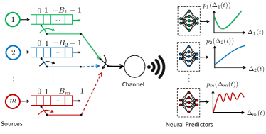
Figure 7: A networked intelligent system, where $m$ sources send features over a shared channel to the corresponding neural predictors. At any time, at most one source can occupy the channel.

Let $G_{l,i}$, $S_{l,i}$, $D_{l,i}$, and $T_{l,i}$ denote the generation time, channel submission time, delivery time, and transmission time duration of the $i$-th feature sent by source $l$, respectively. The feature transmission times $T_{l,i}\geq 1$ are independent across the sources and i.i.d. among the features from the same source. We assume that the $T_{l,i}$’s are not affected by the adopted scheduling policy. The age of information (AoI) of source $l$ at time slot $t$ is given by

$$\Delta_{l}(t) =t-\max_{i}\{G_{l,i}:D_{l,i}\leq t\}.$$ (44)

Our goal is to minimize the time-average weighted sum of the inference errors of the $m$ sources, which is formulated by

$$\!\!\inf_{\pi\in\Pi}\limsup_{T\rightarrow\infty}\frac{1}{T}\sum_{l=1}^{m}w_{l}~{}\mathbb{E}_{\pi}\left[\sum_{t=0}^{T-1}p_{l}(\Delta_{l}(t))\right],$$ (45)

$$\ \text{s.t.}\ \sum_{l=1}^{m}\sum_{b_{l}=0}^{B_{l}-1}c_{l,b_{l}}(t)\leq 1,~{}~{}t=0,1,2,\ldots,$$ (46)

where $p_{l}(\Delta_{l}(t))$ is the inference error of source $l$ at time slot $t$ and $w_{l}>0$ is the weight of source $l$.

V-B Multiple-source Scheduling

Problem (45) can be cast as a Restless Multi-arm Bandit (RMAB) problem by viewing the features stored in the source buffers as arms, where $(l,b_{l})$ is an arm associated with the $(b_{l}+1)$-th freshest feature of the source $l$ and the state of the arm $(l,b_{l})$ is the AoI $\Delta_{l}(t)$ in (44). Finding the optimal solution for RMAB is generally PSPACE hard [43]. Next, we develop a low-complexity scheduling policy by using both Gittins and Whittle indices.

By relaxing the per-slot channel constraint (46) as the following time-average expected channel constraint

$$\limsup_{T\to\infty}\frac{1}{T}\sum_{t=0}^{T-1}\sum_{l=1}^{m}\sum_{b_{l}=0}^{B_{l}-1}\mathbb{E}[c_{l,b_{l}}(t)]\leq 1,$$ (47)

and taking the Lagrangian dual decomposition of the relaxed scheduling problem (45) and (47), we obtain following per-arm scheduling problem:

$$\!\!\!\!\inf_{\pi_{l,b_{l}}\in\Pi_{l,b_{l}}}\limsup_{T\rightarrow\infty}\frac{1}{T}\mathbb{E}_{\pi_{l,b_{l}}}\left[\sum_{t=0}^{T-1}\!w_{l}p_{l}(\Delta_{l}(t))\!+\!\lambda c_{l,b_{l}}(t)\right],\!$$ (48)

where $\Pi_{l,b_{l}}$ is the set of all causal scheduling policies of arm $(l,b_{l})$.

Definition 3 (Indexability).

[44] Let $\Omega_{l,b_{l}}(\lambda)$ be the set of all AoI values $\delta$ such that if the channel is idle and $\Delta_{l}(t)=\delta$, the optimal action to (48) is $d_{l,b_{l}}(t)=0$. Then, the arm $(l,b_{l})$ is indexable if $\lambda_{1}\leq\lambda_{2}$ implies $\Omega_{l,b_{l}}(\lambda_{1})\subseteq\Omega_{l,b_{l}}(\lambda_{2})$.

Algorithm 1 Whittle Index Policy with Selection-from-Buffer

1:Do forever:

2:Update $\Delta_{l}(t)$ for all $l\in\{1,2,\ldots m\}$.

3:Calculate the Whittle index $W_{l,b_{l}}(\Delta_{l}(t))$ for all $l\in\{1,2,\ldots m\}$ and $b_{l}\in\{0,1,\ldots,B_{l}-1\}$ using (7)-(51).

4:if the channel is idle and $\max_{l,b_{l}}W_{l,b_{l}}(\Delta_{l}(t))\geq 0$ then

5:     $(l^{*},b_{l^{*}}^{*})\leftarrow\arg\max_{l,b_{l}}W_{l,b_{l}}(\Delta_{l}(t))$.

6:     Source $l^{*}$ submits its feature $X_{l^{*},t-b_{l^{*}}^{*}}$ to the channel.

7:else

8:     No source is scheduled, even if the channel is idle.

9:end if

Theorem 6.

If $|p_{l}(\delta)|\leq M$ for all $\delta$ and the $T_{l,i}$’s are independent across the sources and i.i.d. among the features from the same source with a finite mean $\mathbb{E}[T_{l,i}]$, then all arms are indexable.

Proof.

See Appendix VIII-N. ∎

Given indexability, the Whittle index $W_{l,b_{l}}(\delta)$ [44] of the arm $(l,b_{l})$ at state $\delta$ is $W_{l,b_{l}}(\delta)=\inf\{\lambda\in\mathbb{R}:\delta\in\Omega_{l,b_{l}}(\lambda)\}$.

Theorem 7.

If the conditions of Theorem 6 hold, then the Whittle index $W_{l,b_{l}}(\delta)$ is given by

$$W_{l,b_{l}}(\delta)\!= \frac{w_{l}}{\mathbb{E}[T_{l,1}]}~{}\mathbb{E}\left[z(T_{l,1},b_{l},\delta)+T_{l,2}\right]~{}\gamma_{l}(\delta)$$

$$-\frac{w_{l}}{\mathbb{E}[T_{l,1}]}~{}\mathbb{E}\left[\sum_{t=T_{l,1}}^{T_{l,1}+z(T_{l,1},b_{l},\delta)+T_{l,2}-1}\!\!\!\!\!\!p_{l}(t+b_{l})\right],$$ (49)

where $\gamma_{l}(\delta)$ is the Gittins index of an AoI bandit process for source $l$, determined by

$$\gamma_{l}(\delta)=\inf_{\tau\in\{1,2,\ldots\}}\frac{1}{\tau}\sum_{k=0}^{\tau-1}\mathbb{E}\left[p_{l}(\delta+k+T_{l,2})\right],$$ (50)

and

$$z(T_{l,1},b_{l},\delta)=\inf_{z\in\mathbb{Z}}\{z\geq 0:\gamma_{l}(T_{l,1}+b_{l}+z)\geq\gamma_{l}(\delta)\}.$$ (51)

Proof.

See Appendix VIII-O. ∎

Finding a (semi-)analytical expression of the Whittle index for minimizing non-monotonic AoI functions is in a challenging task. In Theorem 7, this challenge is resolved by using the Gittins index $\gamma_{l}(\delta)$ to solve (48), where the solution techniques of (32) are employed. The Whittle index scheduling policy for reducing the weighted-sum inference error is described in Algorithm 1, where all sources remain silent when the channel is idle, if $W_{l,b_{l}}(\Delta_{l}(t))<0$ for all $l$ and $b_{l}$.

In the special case that (i) the AoI function $p(\cdot)$ is non-decreasing and (ii) the transmission time is fixed as $T_{l,i}=1$, it holds that $\gamma_{l}(\delta)=p_{l}(\delta+1)$ and $z(T_{l,1},b_{l},\delta)=\max\{\delta-b_{l}-1,0\}$. Hence,

$$W_{l,0}(\delta)=w_{l}\left[\delta~{}p_{l}(\delta+1)-\sum_{t=1}^{\delta}p_{l}(t)\right]$$ (52)

for $\delta\geq 1$ and $b_{l}=0$. By this, the Whittle index in Section IV of [8, Equation (7)] is recovered from Theorem 7.

VI Data Driven Evaluations

In this section, we illustrate the performance of our scheduling policies, where the inference error function $p(\delta)$ is collected from the data driven experiments in Section III-C.

VI-A Single-source Scheduling Policies

We evaluate the following four single-source scheduling policies:

• Generate-at-will, zero wait: The $(i+1)$-th feature sending time $S_{i+1}$ is given by $S_{i+1}=D_{i}=S_{i}+T_{i}$ and the feature selection policy is $f=(0,0,\ldots)$, i.e., $b_{i}=0$ for all $i$.

• Generate-at-will, optimal scheduling: The policy is given by Theorem 4 with $b_{i}=0$ for all $i$.

• Selection-from-buffer, optimal scheduling: The policy is given by Theorem 5.

• Periodic feature updating: Features are generated periodically with a period $T_{p}$ and appended to a queue with buffer size $B$. When the buffer is full, no new feature is admitted to the buffer. Features in the buffer are sent over the channel in a first-come, first-served order.

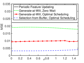
Figure 8: Time average inference error (MSE) vs. the scale parameter $\sigma$ of discretized i.i.d. log-normal transmission time distribution for single-source scheduling (in robot state prediction task).

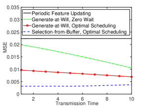
Figure 9: Time average inference error (MSE) vs. Constant Transmission Time (in robot state prediction task).

Figure 10: Time-average weighted sum of the inference errors (Normalized MSE) vs. the weight $w_{1}$ of Source 1 for multi-source scheduling, where the number of sources is $m=2$ and the weight of Source 2 is $w_{2}=1$.

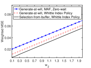
Figure 11: Time-average weighted sum of the inference errors (MSE) vs. the weight $w_{2}$ of Source 2 for multi-source scheduling, where the number of sources is $m=2$ and the weight of Source 2 is $w_{1}=1$.

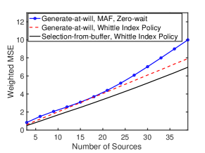
Figure 12: Time-average weighted sum of the inference errors (MSE) vs. number of sources.

Fig. 8 illustrates the time-average inference error achieved by the four single-source scheduling policies defined above. The inference error function $p(\delta)$ used in this evaluation is illustrated in Fig. 3(c), which is generated by using the leader-follower robotic dataset and the trained neural network as explained in Section III-C. The $i$-th feature transmission time $T_{i}$ is assumed to follow a discretized i.i.d. log-normal distribution. In particular, $T_{i}$ can be expressed as $T_{i}=\lceil\alpha e^{\sigma Z_{i}}/\mathbb{E}[e^{\sigma Z_{i}}]\rceil$, where $Z_{i}$’s are i.i.d. Gaussian random variables with zero mean and unit variance. In Fig. 8, we plot the time average inference error versus the scale parameter $\sigma$ of discretized i.i.d. log-normal distribution, where $\alpha=1.2$, the buffer size is $B=30$, and the period of uniform sampling is $T_{p}=3$. The randomness of the transmission time increases with the growth of $\sigma$. Data-driven evaluations in Fig. 8 show that “selection-from-buffer” with optimal scheduler achieves $3$ times performance gain compared to “generate-at-will,” and $8$ times performance gain compared to periodic feature updating.

Fig. 9 illustrates the performance of the four scheduling policies versus constant transmission time $T$. Similar to Fig. 8, the inference error function $p(\delta)$ is measured from leader-follower robotic dataset. This figure also shows that “selection-from-buffer” with optimal scheduler can achieve $8$ time performance gain compared to periodic feature updating.

VI-B Multiple-source Scheduling Policies

Now, we evaluate the following three multiple-source scheduling policies:

• Generate-at-will, maximum age first (MAF), zero wait: At time slot $t$, if the channel is free, this policy will schedule the freshest generated feature from source $\arg\max_{l}\Delta_{l}(t)$; otherwise no source is scheduled.

• Generate-at-will, Whittle index policy: Denote

  $$W_{0}(t)=\max_{l}\!W_{l,0}(\Delta_{l}(t)),~{}l_{0}^{*}=\arg\max_{l}\!W_{l,0}(\Delta_{l}(t)).$$ (53)

  If the channel is free and $W_{0}(t)\geq 0$, the freshest feature of the source $l_{0}^{*}$ is scheduled; otherwise no source is scheduled.

• Selection-from-buffer, Whittle index policy: The policy is described in Algorithm 1.

In Fig. 10, we plot the time average weighted sum of inference errors versus weight $w_{1}$, where the number of sources is $m=2$ and weight $w_{2}=1$. The inference error function $p_{1}(\delta)$ is illustrated in Fig. 3(c). The inference error function $p_{2}(\delta)$ is illustrated in Fig. 1(c), which is generated by using the pre-trained neural network on “BAIR” dataset from [9]. The transmission times for Source 1 and Source 2 are $T_{1,i}=1$ and $T_{2,i}=4$ for all $i$, respectively. The buffer sizes are $B_{1}=B_{2}=30$. The weight $w_{1}$ is associated with a non-monotonic AoI function. The performance gain of “selection-from-buffer, Whittle index policy” increases as $w_{1}$ grows.

Fig. 11 shows the time average weighted sum of inference errors versus weight $w_{2}$, where the weight $w_{1}=1$. The other parameters are the same as in Fig. 10. The weight $w_{2}$ is associated with a monotonic AoI function. The difference among the average weighted sum of inference errors under policies “Selection-from-buffer, Whittle index policy”, “Generate-at-will, Whittle index policy”, and “Generate-at-will, MAF, zero wait” is fixed as $w_{2}$ grows, where “Selection-from-buffer, Whittle index policy” achieves the minimum inference errors.

Fig. 12 depicts the performance of the three scheduling policies as the number of sources $n$ increases. The number of sources is increased from $n=3$ to $n=39$. The number of sources $n$ increments by $3$ in which inference error functions are associated with Fig. 1(c), Fig. 2(c), and Fig. 3(c) with constant transmission times $4,1,$ and $1$, respectively. From Fig. 12, we observe that “Selection-from-buffer, Whittle index policy” achieves minimum inference error than the other two policies.

VII Conclusions

In this paper, we interpreted the impact of data freshness on the performance of real-time supervised learning. We showed that the training error and the inference error of real-time supervised learning could be non-monotonic AoI functions if the target and feature data sequence is far from a Markov model. Our experimental results suggested that the data sequence can be far from Markovian due to response delay, communication delay, and/or long-range dependence. To minimize the time-average inference error, we adopted a new feature transmission model called “selection-from-buffer” and designed an optimal single-source scheduling policy. The optimal single-source scheduling policy is found to be a threshold policy on the Gittins index. Moreover, we developed a Whittle index policy for multiple-source scheduling and provided a semi-analytical expression for the Whittle index. Our numerical results validated the efficacy of the proposed scheduling policies.

VIII Appendix

VIII-A Relationship among $L$-divergence, Bregman divergence, and $f$-divergence

We provide a comparison among the $L$-divergence defined in (8), the Bregman divergence [27], and the $f$-divergence [28].

Let $\mathcal{P^{Y}}$ denote the set of all probability distributions on the discrete set $\mathcal{Y}$. Any distribution $Q_{Y}\in\mathcal{P^{Y}}$ can be represented by a probability vector $\mathbf{q}_{Y}=(Q_{Y}(y_{1}),\ldots,Q_{Y}(y_{|\mathcal{Y}|}))^{T}$ that satisfies $\sum_{y\in\mathcal{Y}}Q_{Y}(y)=1$ and $Q_{Y}(y)\geq 0$ for all $y\in\mathcal{Y}$. If $F:\mathcal{P^{Y}}\mapsto\mathbb{R}$ be a continuously differentiable and strictly convex function, then the Bregman divergence $B_{F}(P_{Y}||Q_{Y})$ between two distributions $P_{Y}\in\mathcal{P^{Y}}$ and $Q_{Y}\in\mathcal{P^{Y}}$ associated with function $F$ is defined by [45]

$$B_{F}(P_{Y}||Q_{Y})=F(\mathbf{p}_{Y})-F(\mathbf{q}_{Y})-\nabla F(\mathbf{q}_{Y})^{T}(\mathbf{p}_{Y}-\mathbf{q}_{Y}),$$ (54)

where $\mathbf{p}_{Y}$ and $\mathbf{q}_{Y}$ are two probability vectors associated to the distributions $P_{Y}$ and $Q_{Y}$, respectively, and $\nabla F(\mathbf{q}_{Y})$ is the gradient of function $F$ at $\mathbf{q}_{Y}$. Consider the loss function

$$L_{F}(y,Q_{Y})=-F(\mathbf{q}_{Y})-\frac{\partial F(\mathbf{q}_{Y})}{\partial P_{Y}(y)}+\nabla F(\mathbf{q}_{Y})^{T}\mathbf{q}_{Y},$$ (55)

where the action $a=Q_{Y}$ is a distribution in $\mathcal{P^{Y}}$.

Lemma 4.

Any Bregman divergence $B_{F}(P_{Y}||Q_{Y})$ is an $L_{F}$-divergence $D_{L_{F}}(P_{Y}||Q_{Y})$, where $L_{F}$ is defined in (55).

Proof.

The $L_{F}$-entropy associated with the loss function $L_{F}(y,Q_{Y})$ in (55) is

$$H_{L_{F}}(Y)=\min_{Q_{Y}\in\mathcal{P^{Y}}}E_{Y\sim P_{Y}}\left[L_{F}\left(Y,Q_{Y}\right)\right],$$ (56)

where $P_{Y}$ is the distribution of $Y$ and

$$E_{Y\sim P_{Y}}\left[L_{F}\left(Y,Q_{Y}\right)\right]=-F(\mathbf{q}_{Y})-\nabla F(\mathbf{q}_{Y})^{T}(\mathbf{p}_{Y}-\mathbf{q}_{Y}).$$ (57)

Because the function $F$ is convex, it follows from (57) that

$$E_{Y\sim P_{Y}}\left[L_{F}\left(Y,Q_{Y}\right)\right]\geq-F(\mathbf{p}_{Y}),\ \forall Q_{Y}\in\mathcal{P^{Y}}.$$ (58)

Moreover, if $Q_{Y}=P_{Y}$, then

$$E_{Y\sim P_{Y}}\left[L_{F}\left(Y,P_{Y}\right)\right]=-F(\mathbf{p}_{Y}).$$ (59)

Combining (56)-(59), it follows that

$$H_{L_{F}}(Y)= E_{Y\sim P_{Y}}\left[L_{F}\left(Y,P_{Y}\right)\right]]=-F(\mathbf{p}_{Y}).$$ (60)

Due to the strict convexity of function $F$, $Q_{Y}=P_{Y}$ is the unique minimizer of (56). Then, by the definition of $L$-divergence in (8), we get

$$D_{L_{F}}(P_{Y}||Q_{Y})$$

$$= E_{Y\sim P_{Y}}\left[L_{F}\left(Y,Q_{Y}\right)\right]-H_{L_{F}}(Y)$$

$$= -F(\mathbf{q}_{Y})-\nabla F(\mathbf{q}_{Y})^{T}(\mathbf{p}_{Y}-\mathbf{q}_{Y})+F(\mathbf{p}_{Y}),$$ (61)

which is equal to the Bregman divergence $B_{F}(P_{Y}||Q_{Y})$ defined in (54). This completes the proof. ∎

By Lemma 4, any Bregman divergence $B_{F}(P_{Y}||Q_{Y})$ is an $L_{F}$-divergence $D_{L_{F}}(P_{Y}||Q_{Y})$. However, the converse is not always true, which is explained below. If $H_{L}(Y)$ is strictly concave and continuously differentiable in $P_{Y}$, then the associated $L$-divergence $D_{L}(P_{Y}||Q_{Y})$ can be expressed as [23, Section 3.5.4]

$$D_{L}(P_{Y}||Q_{Y})$$

$$= H_{L}(\mathbf{q}_{Y})+\nabla H_{L}(\mathbf{q}_{Y})^{T}(\mathbf{p}_{Y}-\mathbf{q}_{Y})-H_{L}(\mathbf{p}_{Y}),$$ (62)

where the $L$-entropy $H_{L}(Y)$ is rewritten as $H_{L}(\mathbf{q}_{Y})$ to emphasize that it is a function of vector $\mathbf{q}_{Y}$. By comparing (VIII-A) with (54), one can observe that the right hand side of (VIII-A) is exactly the Bregman divergence $B_{-H_{L}}(P_{Y}||Q_{Y})$ associated with function $-H_{L}$. If $H_{L}(Y)$ is not strictly concave or not continuously differentiable in $P_{Y}$, then the $L$-divergence $D_{L}(P_{Y}||Q_{Y})$ may not be a Bregman divergence.

The $f$-divergence is defined by [28]

$$D_{f}(P_{Y}||Q_{Y})=\sum_{y\in\mathcal{Y}}Q_{Y}(y)f\left(\frac{P_{Y}(y)}{Q(y)}\right),$$ (63)

where $f:(0:\infty)\mapsto\mathbb{R}$ is a convex function satisfying $f(1)=0$. The $f$-mutual information can be expressed by using the $f$-divergence

$$I_{f}(Y;X)=\mathbb{E}_{X\sim P_{X}}[D_{f}(P_{Y|X}||P_{Y})].$$ (64)

The $f$-mutual information is symmetric, i.e., $I_{f}(Y;X)=I_{f}(X;Y).$ However, the $L$-mutual information is non-symmetric in general, except for some special cases. For example, Shannon’s mutual information is defined by

$$I_{\text{log}}(Y;X)=\mathbb{E}_{X\sim P_{X}}[D_{\text{log}}(P_{Y|X}||P_{Y})],$$ (65)

where $D_{\text{log}}(P_{Y}||Q_{Y})$ is the K-L divergence [32]. It is well-known that $I_{\log}(Y;X)=I_{\log}(X;Y)$. An $f$-divergence may not be $L$-divergence and an $L$ divergence may not be $f$-divergence. In fact, K-L divergence $D_{\text{log}}(P_{Y}||Q_{Y})$ and its dual $D_{\text{log}}(Q_{Y}||P_{Y})$ are unique divergences that belong to $f$-divergence and Bregman divergence [45]. Hence, $D_{\text{log}}(P_{Y}||Q_{Y})$ and $D_{\text{log}}(Q_{Y}||P_{Y})$ are also the only divergences belonging to all the three classes of divergences.

VIII-B Examples of Loss function $L$, $L$-entropy, and $L$-cross entropy

Several examples of the loss function $L$, $L$-entropy, and $L$-cross entropy are listed below. More examples can be found in [23, 24, 25].

VIII-B1 Logarithmic Loss (log-loss)

The log-loss function is given by $L_{\text{log}}(y,Q_{Y})=-\log Q_{Y}(y)$, where the action $a=Q_{Y}$ is a distribution in $\mathcal{P}^{\mathcal{Y}}$. The corresponding $L$-entropy is the well-known Shannon’s entropy [32],

$$H_{\text{log}}(Y)= -\sum_{y\in\mathcal{Y}}P_{Y}(y)\ \text{log}\ P_{Y}(y),$$ (66)

where $P_{Y}$ is the distribution of $Y$. The corresponding $L$-cross entropy is

$$H_{\text{log}}(Y;\tilde{Y})= -\sum_{y\in\mathcal{Y}}P_{Y}(y)\ \text{log}\ P_{\tilde{Y}}(y).$$ (67)

The $L$-mutual information and $L$-divergence associated to the log-loss are Shannon’s mutual information and the K-L divergence, respectively.

VIII-B2 Brier Loss

The Brier loss function is defined as $L_{B}(y,Q_{Y})=\sum_{y^{\prime}\in\mathcal{Y}}Q_{Y}(y^{\prime})^{2}-2\ Q_{Y}(y)+1$ [23]. The associated $L$-entropy is

$$H_{B}(Y)= 1-\sum_{y\in\mathcal{Y}}P_{Y}(y)^{2},$$ (68)

and the associated $L$-cross entropy is

$$H_{B}(Y;\tilde{Y})= \sum_{y\in\mathcal{Y}}P_{\tilde{Y}}(y)^{2}-2\sum_{y\in\mathcal{Y}}P_{\tilde{Y}}(y)P_{Y}(y)+1.$$ (69)

VIII-B3 0-1 Loss

The 0-1 loss function is given by $L_{\text{0-1}}(y,\hat{y})=\mathbf{1}(y\neq\hat{y})$, where $\mathbf{1}(A)$ is the indicator function of event $A$. For this case, we have

$$H_{\text{0-1}}(Y)~{}= ~{}1-\max_{y\in\mathcal{Y}}P_{Y}(y),$$ (70)

$$H_{\text{0-1}}(Y;\tilde{Y})~{}= ~{}1-P_{Y}\left(\arg\max_{y\in\mathcal{Y}}P_{\tilde{Y}}(y)\right).$$ (71)

VIII-B4 $\alpha$-Loss

The $\alpha$-loss function is defined by $L_{\alpha}(y,Q_{Y})=\frac{\alpha}{\alpha-1}\left[1-Q_{Y}(y)^{\frac{\alpha-1}{\alpha}}\right]$ for $\alpha>0$ and $\alpha\neq 1$ [46, Eq. 14]. It becomes the log-loss function at the limit $\alpha\rightarrow 1$ and the 0-1 loss function as the limit $\alpha\rightarrow\infty$. The $L$-entropy and $L$-cross entropy associated to the $\alpha$-loss function are given by

$$H_{\alpha\text{-loss}}(Y)=\frac{\alpha}{\alpha-1}\left[1-\left(\sum_{y\in\mathcal{Y}}P_{Y}(y)^{\alpha}\right)^{\frac{1}{\alpha}}\right],$$ (72)

$$H_{\alpha\text{-loss}}(Y;\tilde{Y})=\frac{\alpha}{\alpha-1}\left[1-\left(\sum_{y\in\mathcal{Y}}P_{\tilde{Y}}(y)^{\alpha}\right)^{\frac{1}{\alpha}}\lambda\right],$$ (73)

where

$$\lambda=\frac{\sum_{y\in\mathcal{Y}}\frac{P_{Y}(y)}{P_{\tilde{Y}}(y)}P_{\tilde{Y}}(y)^{\alpha}}{\sum_{y\in\mathcal{Y}}P_{\tilde{Y}}(y)^{\alpha}}.$$ (74)

VIII-B5 Quadratic Loss

The quadratic loss function is $L_{2}(y,\hat{y})=(y-\hat{y})^{2}$. The $L$-entropy function associated with the quadratic loss is the variance of $Y$, i.e.,

$$H_{2}(Y)=\mathbb{E}[Y^{2}]-\mathbb{E}[Y]^{2}.$$ (75)

The corresponding $L$-cross entropy is

$$H_{2}(Y;\tilde{Y})=\mathbb{E}[Y^{2}]-2\mathbb{E}[\tilde{Y}]\mathbb{E}[Y]+\mathbb{E}[\tilde{Y}]^{2}.$$ (76)

VIII-C Proof of Equation (7)

From (II-B), we get

$$H_{L}(\tilde{Y}_{0}|\tilde{X}_{-\Theta},\Theta)$$

$$= \sum_{\begin{subarray}{c}x\in\mathcal{X},\theta\in\mathcal{D}\end{subarray}}\!\!\!\!P_{\tilde{X}_{-\Theta},\Theta}(x,\theta)H_{L}(\tilde{Y}_{0}|\tilde{X}_{-\Theta}=x,\Theta=\theta)$$

$$\!\!\!\!= \!\!\!\sum_{\theta\in\mathcal{D}}P_{\Theta}(\theta)\sum_{x\in\mathcal{X}}P_{\tilde{X}_{-\Theta}|\Theta=\theta}(x)H_{L}(\tilde{Y}_{0}|\tilde{X}_{-\Theta}=x,\Theta=\theta)\!\!\!$$

$$\!\!\!= \!\!\!\sum_{\theta\in\mathcal{D}}P_{\Theta}(\theta)\sum_{x\in\mathcal{X}}P_{\tilde{X}_{-\theta}|\Theta=\theta}(x)H_{L}(\tilde{Y}_{0}|\tilde{X}_{-\Theta}=x,\Theta=\theta).\!\!\!\!$$ (77)

Next, from (4), we obtain that for all $x\in\mathcal{X}$ and $\theta\in\mathcal{D}$

$$\!\!\!H_{L}(\tilde{Y}_{0}|\tilde{X}_{-\Theta}=x,\Theta=\theta)\!\!= \min_{a\in\mathcal{A}}\!\mathbb{E}_{Y\sim P_{\tilde{Y}_{0}|\tilde{X}_{-\Theta}=x,\Theta=\theta}}[L(Y,a)]\!\!\!$$

$$\!\!= \min_{a\in\mathcal{A}}\!\mathbb{E}_{Y\sim P_{\tilde{Y}_{0}|\tilde{X}_{-\theta}=x,\Theta=\theta}}[L(Y,a)].\!\!\!$$ (78)

Because $\tilde{Y}_{0}$ and $\tilde{X}_{-\theta}$ are independent of $\Theta$, for all $x\in\mathcal{X},y\in\mathcal{Y}$, and all $\theta=0,1,\ldots$

$$P_{\tilde{Y}_{0}|\tilde{X}_{-\theta}=x,\Theta=\theta}(y)=P_{\tilde{Y}_{0}|\tilde{X}_{-\theta}=x}(y).$$ (79)

Hence, (VIII-C) can be simplified as

$$H_{L}(\tilde{Y}_{0}|\tilde{X}_{-\Theta}=x,\Theta=\theta)= \min_{a\in\mathcal{A}}\!\mathbb{E}_{Y\sim P_{\tilde{Y}_{0}|\tilde{X}_{-\theta}=x}}[L(Y,a)]$$

$$= H_{L}(\tilde{Y}_{0}|\tilde{X}_{-\theta}=x).$$ (80)

Substituting (VIII-C) and (79) into (VIII-C), we observe that

$$H_{L}(\tilde{Y}_{0}|\tilde{X}_{-\Theta},\Theta)= \sum_{\theta\in\mathcal{D}}P_{\Theta}(\theta)\sum_{x\in\mathcal{X}}P_{\tilde{X}_{-\theta}}(x)H_{L}(\tilde{Y}_{0}|\tilde{X}_{-\theta}=x)$$

$$= \sum_{\theta\in\mathcal{D}}P_{\Theta}(\theta)~{}H_{L}(\tilde{Y}_{0}|\tilde{X}_{-\theta}).$$ (81)

VIII-D Proof of Equation (11)

The expected inference error in time slots $0,1,\ldots,T-1$ is expressed as

$$\mathrm{err}_{\mathrm{inference}}(T)$$

$$= \frac{1}{T}\sum_{t=1}^{T}\!\mathbb{E}_{Y,X,\Delta\sim P_{Y_{t},X_{t-\Delta(t)},\Delta(t)}}\!\!\left[\!L\left(Y,\phi^{*}_{P_{\tilde{Y}_{0},\tilde{X}_{-\Theta},\Theta}}(X,\Delta)\right)\right],$$

$$= \frac{1}{T}\sum_{t=1}^{T}\bigg{(}\sum_{\delta\in\mathcal{D}}P(\Delta(t)=\delta)$$

$$\times\mathbb{E}_{Y,X\sim P_{Y_{t},X_{t-\Delta(t)}|\Delta(t)=\delta}}\!\!\left[\!L\left(Y,\phi^{*}_{P_{\tilde{Y}_{0},\tilde{X}_{-\Theta},\Theta}}(X,\delta)\right)\right]\bigg{)},$$ (82)

where the empirical distribution $P(\Delta(t)=\delta)$ is equal to $\mathbf{1}(\Delta(t)=\delta)$, which is an indicator function.

Because $Y_{t}$ and $X_{t-\delta}$ are independent of $\Delta(t)$, for all $x\in\mathcal{X},y\in\mathcal{Y}$, and all $\delta\in\mathcal{D}$, we have

$$P_{Y_{t},X_{t-\Delta(t)}|\Delta(t)=\delta}(y,x)= P_{Y_{t},X_{t-\delta}|\Delta(t)=\delta}(y,x)$$

$$= P_{Y_{t},X_{t-\delta}}(y,x).$$ (83)

Hence,

$$\mathbb{E}_{Y,X\sim P_{Y_{t},X_{t-\Delta(t)}|\Delta(t)=\delta}}\!\!\left[\!L\left(Y,\phi^{*}_{P_{\tilde{Y}_{0},\tilde{X}_{-\Theta},\Theta}}(X,\delta)\right)\right]$$

$$= \mathbb{E}_{Y,X\sim P_{Y_{t},X_{t-\delta}|\Delta(t)=\delta}}\!\!\left[\!L\left(Y,\phi^{*}_{P_{\tilde{Y}_{0},\tilde{X}_{-\Theta},\Theta}}(X,\delta)\right)\right]$$

$$= \mathbb{E}_{Y,X\sim P_{Y_{t},X_{t-\delta}}}\!\!\left[\!L\left(Y,\phi^{*}_{P_{\tilde{Y}_{0},\tilde{X}_{-\Theta},\Theta}}(X,\delta)\right)\right].$$ (84)

Now, substituting (VIII-D) into (VIII-D), we obtain (11).

VIII-E Proof of Lemma 1

By using the definition of $\chi^{2}$-conditional mutual information in (16) and [31], we can get

$$I_{\chi^{2}}(Z;Y|X)$$

$$=\sum_{x\mathcal{X},y\in\mathcal{Y}}P_{X,Y}(x,y)\sum_{z\in\mathcal{Z}}\frac{\left(P_{Z|X,Y}(z|x,y)-P_{Z|X}(z|x)\right)^{2}}{P_{Z|X}(z|x)}$$

$$=\!\!\!\!\!\!\!\!\sum_{x\in\mathcal{X},y\in\mathcal{Y},z\in\mathcal{Z}}\!\!\!\!\!P_{X}(x)\frac{\left(P_{Z,Y|X}(z,y|x)\!\!-\!P_{Z|X}(z|x)P_{Y|X}(y|x)\right)^{2}}{P_{Z|X}(z|x)P_{Y|X}(y|x)}$$

$$=\!\!\!\sum_{x\in\mathcal{X},z\in\mathcal{Z}}\!\!\!P_{X,Z}(x,z)\sum_{y\in\mathcal{Y}}\frac{\left(P_{Y|X,Z}(y|x,z)-P_{Y|X}(y|x)\right)^{2}}{P_{Y|X}(y|x)}$$

$$=I_{\chi^{2}}(Y;Z|X).$$ (85)

If $Z\overset{\epsilon}{\rightarrow}X\overset{\epsilon}{\rightarrow}Y$, then by the definition of $\epsilon$-Markov chain in Section III-A and (VIII-E),

$$I_{\chi^{2}}(Z;Y|X)=I_{\chi^{2}}(Y;Z|X)\leq\epsilon^{2}.$$ (86)

Hence, we get $Y\overset{\epsilon}{\rightarrow}X\overset{\epsilon}{\rightarrow}Z$. This completes the proof.

VIII-F Proof of Lemma 2

By the definition of $L$-conditional mutual information in (II-B), we obtain

$$H_{L}(Y|X,Z)= H_{L}(Y|X)-I_{L}(Y;Z|X)$$

$$= H_{L}(Y|Z)-I_{L}(Y;X|Z).$$ (87)

From (II-B) and (VIII-F), we get

$$H_{L}(Y|X)= H_{L}(Y|Z)+I_{L}(Y;Z|X)-I_{L}(Y;X|Z)$$

$$\leq H_{L}(Y|Z)+I_{L}(Y;Z|X),$$ (88)

where the last inequality is due to $I_{L}(Y;X|Z)\geq 0$. Now, it remains to show that if $Y\overset{\epsilon}{\leftrightarrow}X\overset{\epsilon}{\leftrightarrow}Z$, then

$$I_{L}(Y;Z|X)=O(\epsilon);$$ (89)

in addition, if $H_{L}(Y)$ is twice differentiable, then

$$I_{L}(Y;Z|X)=O(\epsilon^{2}).$$ (90)

By using the definition of $L$-conditional mutual information from (II-B), we see that

$$I_{L}(Y;Z|X)= \mathbb{E}_{X,Z}[D_{L}(P_{Y|X,Z}||P_{Y|X})].$$ (91)

If $Y\overset{\epsilon}{\leftrightarrow}X\overset{\epsilon}{\leftrightarrow}Z$ is an $\epsilon$-Markov chain, then

$$\sum_{(x,z)\in\mathcal{X}\times\mathcal{Z}}P_{X,Z}(x,z)D_{\chi^{2}}(P_{Y|X=x,Z=z}||P_{Y|X=x})\leq\epsilon^{2}.$$ (92)

Because the left side of the above inequality is the summation of non-negative terms, the following holds

$$P_{X,Z}(x,z)D_{\chi^{2}}(P_{Y|X=x,Z=z}||P_{Y|X=x})\leq\epsilon^{2},$$ (93)

for all $(x,z)\in\mathcal{X}\times\mathcal{Z}$.

If $P_{X,Z}(x,z)>0$, then

$$D_{\chi^{2}}(P_{Y|X=x,Z=z}||P_{Y|X=x})\leq\dfrac{\epsilon^{2}}{P_{X,Z}(x,z)}.$$ (94)

Next, we need the following lemma.

Lemma 5.

The following assertions are true:

• If two distributions $Q_{Y},P_{Y}\in\mathcal{P^{Y}}$ satisfy

  $$D_{\chi^{2}}(P_{Y}||Q_{Y})\leq\beta^{2},$$ (95)

  then

  $$D_{L}(P_{Y}||Q_{Y})=O(\beta).$$ (96)

• If, in addition, $H_{L}(Y)$ is twice differentiable in $P_{Y}$, then

  $$D_{L}(P_{Y}||Q_{Y})=O(\beta^{2}).$$ (97)

Proof.

See in Appendix VIII-P. ∎

Define set $\hat{\mathcal{X}}\times\hat{\mathcal{Z}}=\{(x,z)\in\mathcal{X}\times\mathcal{Z}:P_{X,Z}(x,z)>0\}$. Then, using (94) and Lemma 5(a) in (91), we obtain

$$I_{L}(Y;Z|X)$$

$$= \sum_{(x,z)\in\mathcal{X}\times\mathcal{Z}}P_{X,Z}(x,z)~{}D_{L}(P_{Y|X=x,Z=z}||P_{Y|X=x})$$

$$= \sum_{(x,z)\in\hat{\mathcal{X}}\times\hat{\mathcal{Z}}}P_{X,Z}(x,z)~{}D_{L}(P_{Y|X=x,Z=z}||P_{Y|X=x})$$

$$= \sum_{(x,z)\in\hat{\mathcal{X}}\times\hat{\mathcal{Z}}}P_{X,Z}(x,z)~{}O\left(\frac{\epsilon}{\sqrt{P_{X,Z}(x,z)}}\right)$$

$$= ~{}O(\epsilon).$$ (98)

Similarly, when $H_{L}(Y)$ is differentiable in $P_{Y}$, by using Lemma 5(b) we obtain

$$I_{L}(Y;Z|X)=O(\epsilon^{2}).$$ (99)

This completes the proof of Lemma 2.

VIII-G Proof of Theorem 1

By using the definition of the $L$-conditional mutual information (II-B), we can show that

$$H_{L}(\tilde{Y}_{0}|\tilde{X}_{-k},\tilde{X}_{-k-1})$$

$$= H_{L}(\tilde{Y}_{0}|\tilde{X}_{-k-1})-I_{L}(\tilde{Y}_{0};\tilde{X}_{-k}|\tilde{X}_{-k-1})$$

$$= H_{L}(\tilde{Y}_{0}|\tilde{X}_{-k})-I_{L}(\tilde{Y}_{0};\tilde{X}_{-k-1}|\tilde{X}_{-k}).$$ (100)

We can expand $H_{L}(\tilde{Y}_{0}|\tilde{X}_{-k})$ as

$$H_{L}(\tilde{Y}_{0}|\tilde{X}_{-k})= H_{L}(\tilde{Y}_{0}|\tilde{X}_{-k-1})+I_{L}(\tilde{Y}_{0};\tilde{X}_{-k-1}|\tilde{X}_{-k})$$

$$-I_{L}(\tilde{Y}_{0};\tilde{X}_{-k}|\tilde{X}_{-k-1}).$$ (101)

As the above equation is valid for all values of $k$, taking the summation of $H_{L}(\tilde{Y}_{0}|\tilde{X}_{-k})$ from $k=0$ to $\theta-1$ yields

$$H_{L}(\tilde{Y}_{0}|\tilde{X}_{-\theta})= H_{L}(\tilde{Y}_{0}|\tilde{X}_{0})+\sum_{k=0}^{\theta-1}I_{L}(\tilde{Y}_{0};\tilde{X}_{-k}|\tilde{X}_{-k-1})$$

$$-\sum_{k=0}^{\theta-1}I_{L}(\tilde{Y}_{0};\tilde{X}_{-k-1}|\tilde{X}_{-k}).$$ (102)

Thus, we can write $H_{L}(\tilde{Y}_{0}|\tilde{X}_{-\theta})$ as a function of $\theta$ as in (20) and (1). Moreover, the functions $g_{1}(\theta)$ and $g_{2}(\theta)$ defined in (1) are non-decreasing of $\theta$ as $I_{L}(\tilde{Y}_{0};\tilde{X}_{-k}|\tilde{X}_{-k-1})\geq 0$ and $I_{L}(\tilde{Y}_{0};\tilde{X}_{-k-1}|\tilde{X}_{-k})\geq 0$ for all values of $k$.

To prove the next part, we use Lemma 2. Because for every $\mu,\nu\geq 0$, $\tilde{Y}_{0}\overset{\epsilon}{\leftrightarrow}\tilde{X}_{-\mu}\overset{\epsilon}{\leftrightarrow}\tilde{X}_{-\mu-\nu}$ is an $\epsilon$-Markov chain, we can write

$$I_{L}(\tilde{Y}_{0};\tilde{X}_{-k-1}|\tilde{X}_{-k})=O(\epsilon).$$ (103)

This implies

$$g_{2}(\theta)=\sum_{k=0}^{\theta-1}O(\epsilon)=O(\epsilon).$$ (104)

The last equality is due to the summation property of big-O-notation.

VIII-H Proof of Theorem 2

Using (7) and Theorem 1, we obtain

$$H_{L}(\tilde{Y}_{0}|\tilde{X}_{-\Theta},\Theta)$$

$$= \sum_{\theta\in\mathcal{D}}\!P_{\Theta}(\theta)\big{(}H_{L}(\tilde{Y}_{0}|\tilde{X}_{0})+\!\hat{g}_{1}(\theta)-g_{2}(\theta)\big{)}$$

$$= H_{L}(\tilde{Y}_{0}|\tilde{X}_{0})\!+\mathbb{E}_{\Theta\sim P_{\Theta}}\![\hat{g}_{1}(\Theta)]\!-\mathbb{E}_{\Theta\sim P_{\Theta}}\![g_{2}(\Theta)],$$ (105)

where

$$\hat{g}_{1}(\theta) =g_{1}(\theta)-H_{L}(\tilde{Y}_{0}|\tilde{X}_{0})$$

$$=\sum_{k=0}^{\theta-1}I_{L}(\tilde{Y}_{0};\tilde{X}_{-k}|\tilde{X}_{-k-1}).$$ (106)

Because mutual information $I_{L}(\tilde{Y}_{0};\tilde{X}_{-k}|\tilde{X}_{-k-1})$ is non-negative,

$$\hat{g}_{1}(\theta)=\sum_{k=0}^{\theta-1}I_{L}(\tilde{Y}_{0};\tilde{X}_{-k}|\tilde{X}_{-k-1})\geq 0.$$ (107)

Because $\hat{g}_{1}(\theta)$ is non-negative for all $\theta$, the function $\hat{g}_{1}(\cdot)$ is Lebesgue integrable with respect to all probability measure $P_{\Theta}$ [47]. Hence, the expectation $\mathbb{E}_{\Theta\sim P_{\Theta}}[\hat{g}_{1}(\Theta)]$ exist. Note that $E_{\Theta\sim P_{\Theta}}[\hat{g}_{1}(\Theta)]$ can be infinite ($+\infty$). By using the same argument, we get that $E_{\Theta\sim P_{\Theta}}[g_{2}(\Theta)]$ exists, but can be infinite. Moreover, the function $\hat{g}_{1}(\theta)$ and $g_{2}(\theta)$ is non-decreasing in $\theta$.

Because (i) the function $\hat{g}_{1}(\theta)$ is non-decreasing in $\theta$, (ii) the expectation $\mathbb{E}_{\Theta\sim P_{\Theta}}[\hat{g}_{1}(\Theta)]$ exist, and (iii) $\Theta_{1}\leq_{st}\Theta_{2}$, we get [33]

$$\mathbb{E}_{\Theta\sim P_{\Theta_{1}}}[\hat{g}_{1}(\Theta)]\leq\mathbb{E}_{\Theta\sim P_{\Theta_{2}}}[\hat{g}_{1}(\Theta)].$$ (108)

Next, by using (VIII-H), (108), and Theorem 1(b), we obtain (24):

$$H_{L}(\tilde{Y}_{0}|\tilde{X}_{-\Theta_{1}},\Theta_{1})$$

$$= H_{L}(\tilde{Y}_{0}|\tilde{X}_{0})+\mathbb{E}_{\Theta\sim P_{\Theta_{1}}}[\hat{g}_{1}(\Theta)]-\mathbb{E}_{\Theta\sim P_{\Theta_{1}}}[g_{2}(\Theta)]$$

$$\leq H_{L}(\tilde{Y}_{0}|\tilde{X}_{0})+\mathbb{E}_{\Theta\sim P_{\Theta_{2}}}[\hat{g}_{1}(\Theta)]-\mathbb{E}_{\Theta\sim P_{\Theta_{1}}}[g_{2}(\Theta)]$$

$$= H_{L}(\tilde{Y}_{0}|\tilde{X}_{-\Theta_{2}},\Theta_{2})$$

$$+\mathbb{E}_{\Theta\sim P_{\Theta_{2}}}[g_{2}(\Theta)]-\mathbb{E}_{\Theta\sim P_{\Theta_{1}}}[g_{2}(\Theta)]$$

$$= H_{L}(\tilde{Y}_{0}|\tilde{X}_{-\Theta_{2}},\Theta_{2})+O(\epsilon).$$ (109)

VIII-I Proof of Lemma 3

By using condition (25) and Lemma 5(a), we obtain for all $x\in\mathcal{X}$

$$D_{L}\left(P_{Y_{t}|X_{t-\delta}=x}||P_{\tilde{Y}_{0}|\tilde{X}_{-\delta}=x}\right)=O(\beta).$$ (110)

Next, by using (II-C) and (110), we get

$$H_{L}(Y_{t};\tilde{Y}_{0}|X_{t-\delta})$$

$$= H_{L}(Y_{t}|X_{t-\delta})$$

$$+\sum_{x\in\mathcal{X}}P_{X_{t-\delta}}(x)~{}D_{L}\left(P_{Y_{t}|X_{t-\delta}=x}||P_{\tilde{Y}_{0}|\tilde{X}_{-\delta}=x}\right)$$

$$= H_{L}(Y_{t}|X_{t-\delta})+O(\beta).$$ (111)

VIII-J Proof of Theorem 3

Part (a): By the definition of $L$-conditional cross entropy (II-C), we get

$$H_{L}(Y_{t};\tilde{Y}_{0}|X_{t-\delta})$$

$$= \!\!\!\sum_{x\in\mathcal{X}}\!\!P_{X_{t-\delta}}(x)\mathbb{E}_{Y\sim P_{Y_{t}|X_{t-\delta}=x}}\!\!\left[\!L\left(Y,a_{\tilde{Y}_{0}|\tilde{X}_{-\delta}=x}\right)\right],\!\!$$ (112)

where the Bayes predictor $a_{\tilde{Y}_{0}|\tilde{X}_{-\delta}=x}$ is fixed in the inference phase for every time slot $t$. Because $\{(\tilde{Y}_{t},\tilde{X}_{t}),t\in\mathbb{Z}\}$ is a stationary process, (VIII-J) is a function of the inference AoI $\delta$.

Part (b): By using Lemma 3 and Theorem 1, we get

$$H_{L}(Y_{t};\tilde{Y}_{0}|X_{t-\delta_{1}})= H_{L}(Y_{t}|X_{t-\delta_{1}})+O(\beta)$$

$$\leq H_{L}(Y_{t}|X_{t-\delta_{2}})+O(\epsilon)+O(\beta)$$

$$= H_{L}(Y_{t};\tilde{Y}_{0}|X_{t-\delta_{2}})+O(\beta)+O(\epsilon)+O(\beta)$$

$$= H_{L}(Y_{t};\tilde{Y}_{0}|X_{t-\delta_{2}})+O(\max\{\epsilon,\beta\}).$$ (113)

This completes the proof.

VIII-K Simplification of the Gittins Index in (37)

For the bandit process $\{\Delta(t):t\geq 0\}$ in (33), define the $\sigma$-field

$$\mathcal{F}_{s}^{t}=\sigma(\Delta(t+k):k\in\{0,1,\ldots,s\}),$$ (114)

which is the set of events whose occurrence are determined by the realization of the process $\{\Delta(t+k):k\in\{0,1,\ldots,s\}\}$ from time slot $t$ up to time slot $t+s$. Then, $\{\mathcal{F}_{k}^{t},k\in\{0,1,\ldots\}\}$ is the filtration of the time shifted process $\{\Delta(t+k):k\in\{0,1,\ldots\}\}$. We define $\mathfrak{M}$ as the set of all stopping times by

$$\mathfrak{M}=\{\nu\geq 0:\{\nu=k\}\in\mathcal{F}_{k}^{t},k\in\{0,1,2,\ldots\}\}.$$ (115)

The Gittins index $\gamma(\delta)$ [11] is the value of reward $r$ for which the stop and continue actions are equally profitable at state $\Delta(t)=\delta$. Hence, $\gamma(\delta)$ is the root of the following equation of $r$:

$$\sup_{\nu\in\mathfrak{M},\nu\neq 0}\mathbb{E}\left[\sum_{k=0}^{\nu+T_{1}-1}[r-p(\Delta(t+k))]\bigg{|}\Delta(t)=\delta\right]$$

$$~{}~{}~{}~{}~{}~{}=\mathbb{E}\left[\sum_{k=0}^{T_{1}-1}[r-p(\Delta(t+k))]\bigg{|}\Delta(t)=\delta\right].$$ (116)

where the left hand side of (VIII-K) is the maximum total expected profit under continue action and the right hand side of (VIII-K) is the total expected profit under stop action. By re-arranging (VIII-K), it can be expressed as

$$\sup_{\nu\in\mathfrak{M},\nu\neq 0}\mathbb{E}\left[\sum_{k=0}^{\nu-1}[r-p(\Delta(t+k+T_{1}))]\bigg{|}\Delta(t)=\delta\right]=0.$$ (117)

Because the left hand side of (117) is the supremum of strictly increasing and linear functions of $r$, it is convex, continuous, and strictly increasing in $r$. Thus, the fixed-point equation (117) has a unique root. The root can also be expressed as

$$\gamma(\delta)$$

$$= \bigg{\{}r:\!\!\!\!\sup_{\nu\in\mathfrak{M},\nu\neq 0}\!\!\!\!\mathbb{E}\left[\sum_{k=0}^{\nu-1}[r-p(\Delta(t+k+T_{1}))]\bigg{|}\Delta(t)\!=\!\delta\right]\!\!=\!0\bigg{\}}.$$ (118)

Let $\nu^{*}\in\mathfrak{M}$ be the optimal stopping time that solves (VIII-K). Because of (33) and $T_{1}\geq 1$, for any $k\leq\nu^{*}$, $\Delta(t+k)=\Delta(t)+k$. Hence, $\{\Delta(t+k):1\leq k\leq\nu^{*}\}$ is completely determined by the initial value $\Delta(t)$ and for all $k\leq\nu^{*}$, the $\sigma$-field $\mathcal{F}_{k}^{t}$ can be simplified as $\mathcal{F}_{k}^{t}=\sigma(\Delta(t))$. Thus, any stopping time in $\mathfrak{M}$ is a deterministic time, given $\Delta(t)=\delta$. By this, (VIII-K) can be simplified as

$$\gamma(\delta)$$

$$= \bigg{\{}r:\!\!\!\!\!\sup_{\tau\in\{1,2,\ldots\}}\!\!\!\!\!\mathbb{E}\left[\sum_{k=0}^{\tau-1}[r-p(\Delta(t+k+T_{1}))]\bigg{|}\Delta(t)\!=\!\delta\right]\!\!=\!0\bigg{\}}$$

$$= \bigg{\{}r:\!\!\!\!\!\inf_{\tau\in\{1,2,\ldots\}}\mathbb{E}\left[\sum_{k=0}^{\tau-1}[p(\Delta(t+k+T_{1}))-r]\bigg{|}\Delta(t)\!=\!\delta\right]\!\!=\!0\bigg{\}}$$

$$= \!\bigg{\{}r:\!\!\!\!\!\inf_{\tau\in\{1,2,\ldots\}}\sum_{k=0}^{\tau-1}\!\mathbb{E}\left[p(\Delta(t+k+T_{1}))-r\bigg{|}\!\Delta(t)\!=\delta\right]\!\!=\!0\bigg{\}},$$ (119)

where $\tau$ is a deterministic positive integer.

Define

$$f(r)=\inf_{\tau\in\{1,2,\ldots\}}\sum_{k=0}^{\tau-1}\mathbb{E}\left[p(\delta+k+T_{1})-r\right].$$ (120)

Similar to Lemma 7 in [14], the following lemma holds.

Lemma 6.

$f(r)\lesseqgtr 0$ if and only if

$$\inf_{\tau\in\{1,2,\ldots\}}\frac{1}{\tau}\sum_{k=0}^{\tau-1}\mathbb{E}\left[p(\delta+k+T_{1})\right]\lesseqgtr r.$$ (121)

By (VIII-K), (VIII-K), and Lemma 6, the root of equation $f(r)=0$ is given by (37). This completes the proof.

VIII-L Proof of Theorem 4

The infinite horizon average AoI penalty problem (32) can be cast as a Markov decision problem (MDP). To describe the MDP, we define the action, state, state transition, and penalty function.

• Action: If the channel server is idle, the possible actions taken by the scheduler at time slot $t$ are $d_{b}(t)=0$ “do not send” and $d_{b}(t)=1$ “send”. Then, $S_{i+1}$ is determined by

  $$S_{i+1}=\inf_{t\in\mathbb{Z}}\{t\geq D_{i}:d_{b}(t)=1\}.$$ (122)

  Hence, one can also use $g=(d_{b}(0),d_{b}(1),d_{b}(2),\ldots)$ to represent a policy in $\mathcal{G}$.

• AoI Penalty: The penalty at every time slot $t$ is $p(\Delta(t))$.

• State: The state of the MDP is the age value $\Delta(t)$.

• State Transition: Because $b_{i}=b$ for all $i$, the state $\Delta(t)$ evolves as follows

  $$\Delta(t)=\begin{cases}T_{i}+b,&\text{if}~{}t=D_{i},i=0,1,\ldots,\\ \Delta(t-1)+1,&\text{otherwise}.\end{cases}$$ (123)

Because the state space is countable, action space is finite, and $p(\delta)$ is bounded, if $\Delta(t)=\delta$, then the optimal decision $d_{b}(t)$ in time slot $t$ satisfies the following Bellman optimality equation [48, Section 5.6.3]

$$V_{b}(\delta)=\min_{d_{b}(t)\in\{0,1\}}Q_{b}(\delta,d_{b}(t)),$$ (124)

where the function $V_{b}$ is the relative value function, the relative value $V_{b}(\delta)$ is the expected total cost relative to the optimal average cost $\bar{p}_{b}$ of the problem (32) when starting from state $\delta$ and following an optimal policy, and $Q_{b}(\delta,d_{b}(t))$ is given by

$$Q_{b}(\delta,1)$$

$$=\mathbb{E}\left[\sum_{k=0}^{T_{i+1}-1}[p(\delta+k)-\bar{p}_{b}]\right]+\mathbb{E}[V_{b}(T_{i+1}+b)],$$ (125)

$$Q_{b}(\delta,0)$$

$$=\inf_{\nu\in\mathfrak{M},\nu\neq 0}\mathbb{E}\left[\sum_{k=0}^{\nu+T_{i+1}-1}[p(\delta+k)-\bar{p}_{b}]\right]+\mathbb{E}[V_{b}(T_{i+1}+b)]$$

$$\overset{(a)}{=}\inf_{\tau\in\{1,2,\ldots\}}\mathbb{E}\left[\sum_{k=0}^{\tau+T_{i+1}-1}[p(\delta+k)-\bar{p}_{b}]\right]+\mathbb{E}[V_{b}(T_{i+1}+b)]$$

$$\overset{(b)}{=}\inf_{\tau\in\{1,2,\ldots\}}\mathbb{E}\left[\sum_{k=0}^{\tau-1}[p(\delta+k+T_{i+1})-\bar{p}_{b}]\right]$$

$$+\mathbb{E}\left[\sum_{k=0}^{T_{i+1}-1}[p(\delta+k)-\bar{p}_{b}]\right]+\mathbb{E}[V_{b}(T_{i+1}+b)].$$ (126)

where $\mathfrak{M}$ is the set of all stopping times defined in Appendix VIII-K. As deduced in Appendix VIII-K, given $\Delta(t)=\delta$, the set of all stopping times is $\mathfrak{M}=\{0,1,2,\ldots\}$. We obtain equality (a) because $\mathfrak{M}$ is $\{0,1,2,\ldots\}$ given $\Delta(t)=\delta$. By re-arranging (a), we get equality (b).

By (124), $d_{b}(t)=1$ is optimal, if

$$Q_{b}(\delta,0)-Q_{b}(\delta,1)\geq 0.$$ (127)

The inequality (127) can also be expressed as

$$\inf_{\tau\in\{1,2,\ldots\}}\mathbb{E}\left[\sum_{k=0}^{\tau-1}[p(\delta+k+T_{i+1})-\bar{p}_{b}]\right]\geq 0.$$ (128)

Next, Lemma 6 implies that the inequality (128) holds if and only if

$$\inf_{\tau\in\{1,2,\ldots\}}\frac{1}{\tau}\sum_{k=0}^{\tau-1}\mathbb{E}\left[p(\delta+k+T_{i+1})\right]\geq\bar{p}_{b}.$$ (129)

Now, using (122) and (127)-(129), we get (38).

Since the transmission times $T_{i}$ are i.i.d., similar to [6, Appendix F], we get that the optimal objective value to (32) is

$$\bar{p}_{b}=\frac{\mathbb{E}\left[\sum_{t=D_{i}(\bar{p}_{b})}^{D_{i+1}(\bar{p}_{b})-1}p\big{(}\Delta(t)\big{)}\right]}{\mathbb{E}\left[D_{i+1}(\bar{p}_{b})-D_{i}(\bar{p}_{b})\right]}.$$ (130)

Hence, $\bar{p}_{b}$ is equal to the root of (39). The left hand side of (39) is concave, continuous, and strictly decreasing in $\beta_{b}$ [14]. Hence, the root of (39) is unique. This completes the proof.

VIII-M Proof of Theorem 5

The problem (31) can be cast as an MDP problem. The State and the penalty of the MDP are the same as the MDP discussed in Appendix VIII-L. The action space is different: If the channel is idle, the scheduler sends $(b+1)$-th freshest feature or does not send any feature. Let $d(t)=\textsc{idle}$ means the scheduler does not send feature at time $t$ and $d(t)=b$ means the scheduler sends $(b+1)$-th freshest feature at time $t$. Then, $S_{i+1}$ and $b_{i+1}$ are determined by

$$S_{i+1} =\inf_{t\in\mathbb{Z}}\{t\geq S_{i}+T_{i}:d(t)\neq\textsc{idle}\},$$ (131)

$$b_{i+1} =d(S_{i+1}).$$ (132)

If the channel is idle and $\Delta(t)=\delta$, then the optimal decision $d(t)$ in time slot $t$ satisfies the following Bellman optimality equation

$$V(\delta)=\min_{d(t)\in\{\textsc{idle},0,1,\ldots,B-1\}}Q(\delta,d(t)),$$ (133)

where the function $V$ is the relative value function and $Q(\delta,d(t))$ is given by

$$Q(\delta,b)$$

$$=\mathbb{E}\left[\sum_{k=0}^{T_{i+1}-1}[p(\delta+k)-\bar{p}_{\text{opt}}]\right]+\mathbb{E}[V(T_{i+1}+b)],$$ (134)

$$Q(\delta,\textsc{idle})$$

$$=\inf_{\tau\in\{1,2,\ldots\}}\mathbb{E}\left[\sum_{k=0}^{\tau-1}[p(\delta+k+T_{i+1})-\bar{p}_{\text{opt}}]\right]$$

$$+\mathbb{E}\left[\sum_{k=0}^{T_{i+1}-1}[p(\delta+k)-\bar{p}_{\text{opt}}]\right]+\min_{b\in\mathcal{B}}\mathbb{E}[V(T_{i+1}+b)].$$ (135)

where $\mathcal{B}=\{0,1,\ldots,B-1\}$ and $\bar{p}_{\text{opt}}$ is the optimal value of (31).

By (133), $d(t)=\textsc{idle}$ is not an optimal choice if

$$Q(\delta,\textsc{idle})-\min_{b\in\mathcal{B}}Q(\delta,b)\geq 0.$$ (136)

By using similar steps (127)-(129), we can get that the inequality (136) holds if and only if

$$\gamma(\delta)\geq\bar{p}_{\text{opt}}.$$ (137)

Then, by using (131), (136), and (137), we get the optimal sending time $S^{*}_{i+1}$ in (42).

Next, we need to get the optimal $b^{*}_{i+1}$ and $\bar{p}_{\text{opt}}$. When $\Delta(S^{*}_{i+1})=\delta$, $b^{*}_{i+1}=b^{*}$ is optimal if

$$b^{*}= \arg\min_{b\in\mathcal{B}}Q(\delta,b)$$

$$= \arg\min_{b\in\mathcal{B}}\mathbb{E}\left[\sum_{k=0}^{T_{i+1}-1}[p(\delta+k)-\bar{p}_{\text{opt}}]\right]+\mathbb{E}[V(T_{i+1}+b)]$$

$$= \arg\min_{b\in\mathcal{B}}\mathbb{E}[V(T_{i+1}+b)].$$ (138)

Observe that the optimal $b^{*}$ is independent of the state $\Delta(S_{i+1})=\delta$. Moreover, because $T_{i}$ is identically distributed,

$$\mathbb{E}[V(T_{0}+b)]=\mathbb{E}[V(T_{1}+b)]=\ldots=\mathbb{E}[V(T_{i}+b)],\forall i.$$ (139)

Thus, the optimal $b^{*}$ is constant for all $i$. If $b_{i+1}=b$ for all $i$, then $\bar{p}_{b}$ is the average inference error. Hence, the optimal choice $b^{*}$ satisfies

$$b^{*}=\arg\min_{b\in\mathcal{B}}\bar{p}_{b},$$ (140)

where $\bar{p}_{b}$ is $\beta_{b}$, which is the root of (39). The optimal value is

$$\bar{p}_{\text{opt}}=\min_{b\in\mathcal{B}}\bar{p}_{b}.$$ (141)

VIII-N Proof of Theorem 6

If the channel is idle and $\Delta_{l}(t)=\delta$, the optimal decision $d_{l,b_{l}}(t)$ for the problem (48) in time slot $t$ satisfies the following Bellman optimality equation

$$V_{l,b_{l}}(\delta)=\min_{d_{l,b_{l}}(t)\in\{0,1\}}Q_{l,b_{l}}(\delta,d_{l,b_{l}}(t)),$$ (142)

where the function $V_{l,b_{l}}$ is the relative value function and $Q_{l,b_{l}}(\delta,d_{l,b_{l}}(t))$ is given by

$$Q_{l,b_{l}}(\delta,1)$$

$$=\mathbb{E}\left[\sum_{k=0}^{T_{l,i+1}-1}[w_{l}p_{l}(\delta+k)-\bar{p}_{l,b_{l}}(\lambda)]\right]\!$$ (143)

$$+\!\mathbb{E}[V_{l,b_{l}}(T_{l,i+1}+b_{l})]\!+\!\lambda,$$

$$Q_{l,b_{l}}(\delta,0)$$

$$=\inf_{\tau\in\{1,2,\ldots\}}\mathbb{E}\left[\sum_{k=0}^{\tau-1}[w_{l}p_{l}(\delta+k+T_{l,i+1})-\bar{p}_{l,b_{l}}(\lambda)]\right]$$

$$+\mathbb{E}\left[\sum_{k=0}^{T_{l,i+1}-1}[w_{l}p_{l}(\delta+k)-\bar{p}_{l,b_{l}}(\lambda)]\right]\!$$

$$+\!\mathbb{E}[V_{l,b_{l}}(T_{l,i+1}+b_{l})]\!+\!\lambda.$$ (144)

where $\bar{p}_{l,b_{l}}(\lambda)$ is optimal objective value of the problem (48).

Similar to the proof of (129) and (130) in Section VIII-L, by solving (142), $d_{l,b_{l}}(t)=0$ is optimal if

$$w_{l}~{}\gamma_{l}(\delta)\leq\bar{p}_{l,b_{l}}(\lambda),$$ (145)

otherwise $d_{l,b_{l}}(t)=1$ is optimal, where $\bar{p}_{l,b_{l}}(\lambda)$ is given by

$$\bar{p}_{l,b_{l}}(\lambda)=\frac{C^{l}_{i,i+1}(\lambda)}{N^{l}_{i,i+1}(\lambda)},$$ (146)

where $C^{l}_{i,i+1}(\lambda)$ is the expected penalty of source $l$ starting from $i$-th delivery time to $(i+1)$-th delivery time and $N^{l}_{i,i+1}(\lambda)$ is the expected number of time slots from $i$-th delivery time to $(i+1)$-th delivery time, given by

$$\!\!C^{l}_{i,i+1}(\lambda)\!\!=\!\mathbb{E}\left[\sum_{t=D_{l,i}(\bar{p}_{l,b_{l}}(\lambda))}^{D_{l,i+1}(\bar{p}_{l,b_{l}}(\lambda))-1}\!\!\!\!\!w_{l}p_{l}\big{(}\Delta_{l}(t)\big{)}\right]+\lambda\mathbb{E}[T_{l,i+1}],$$ (147)

$$N^{l}_{i,i+1}(\lambda)=\mathbb{E}\left[D_{l,i+1}(\bar{p}_{l,b_{l}}(\lambda))-D_{l,i}(\bar{p}_{l,b_{l}}(\lambda))\right],$$ (148)

the $(i+1)$-th feature delivery time $D_{l,i+1}(\bar{p}_{l,b_{l}}(\lambda))$ from source $l$ is

$$D_{l,i+1}(\bar{p}_{l,b_{l}}(\lambda))=S_{l,i+1}(\bar{p}_{l,b_{l}}(\lambda))+T_{l,i+1}$$ (149)

and the $(i+1)$-th sending time $S_{l,i+1}(\bar{p}_{l,b_{l}}(\lambda))$ is

$$S_{l,i+1}(\bar{p}_{l,b_{l}}(\lambda))=\inf_{t\in\mathbb{Z}}\{t\geq D_{l,i}:w_{l}~{}\gamma_{l}(\delta)\leq\bar{p}_{l,b_{l}}(\lambda)\}.$$ (150)

The sending time $S_{l,i+1}(\bar{p}_{l,b_{l}}(\lambda))$ can also be expressed as

$$S_{l,i+1}(\bar{p}_{l,b_{l}}(\lambda))=D_{l,i}(\bar{p}_{l,b_{l}}(\lambda))+z(T_{l,i},b_{l},\bar{p}_{l,b_{l}}(\lambda)),$$ (151)

the waiting time $z(T_{l,i},b_{l},\bar{p}_{l,b_{l}}(\lambda))$ after the delivery time $D_{l,i}(\bar{p}_{l,b_{l}}(\lambda))$ is

$$z(T_{l,i},b_{l},\bar{p}_{l,b_{l}}(\lambda))$$

$$= \inf_{z\in\mathbb{Z}}\{z\geq 0:w_{l}~{}\gamma_{l}(\Delta_{l}(D_{l,i}(\bar{p}_{l,b_{l}}(\lambda)))+z)\geq\bar{p}_{l,b_{l}}(\lambda)\}$$

$$= \inf_{z\in\mathbb{Z}}\{z\geq 0:w_{l}~{}\gamma_{l}(T_{l,i}+b_{l}+z)\geq\bar{p}_{l,b_{l}}(\lambda)\},$$ (152)

where the last equality holds because from (44), we get

$$\Delta_{l}(t)=\begin{cases}T_{l,i}+b_{l},&\text{if}~{}t=D_{l,i}(\bar{p}_{l,b_{l}}(\lambda)),i=0,1,\ldots,\\ \Delta_{l}(t-1)+1,&\text{otherwise}.\end{cases}$$ (153)

By using (149)-(153), (147) and (148) reduce to

$$C^{l}_{i,i+1}(\lambda)= \mathbb{E}\left[\sum_{k=T_{l,i}}^{T_{l,i}+z(T_{l,i},b_{l},\bar{p}_{l,b_{l}}(\lambda))+T_{l,i+1}-1}\!\!\!\!\!\!w_{l}~{}p_{l}(k+b_{l})\right]$$

$$+\lambda\mathbb{E}[T_{l,i+1}],$$ (154)

$$N^{l}_{i,i+1}(\lambda)=\mathbb{E}\left[z(T_{l,i},b_{l},\bar{p}_{l,b_{l}}(\lambda))+T_{l,i+1}\right].$$ (155)

Thus, the optimal objective value $\bar{p}_{l,b_{l}}(\lambda)$ is exactly equal to

$$\bar{p}_{l,b_{l}}(\lambda)=\{\beta:f(\beta)+\lambda\mathbb{E}[T_{l,i+1}]=0\},$$ (156)

$$f(\beta)= \mathbb{E}\left[\sum_{k=T_{l,i}}^{T_{l,i}+z(T_{l,i},b_{l},\beta)+T_{l,i+1}-1}\!\!\!\!\!\!w_{l}~{}p_{l}(t+b_{l})\right]$$

$$-\beta~{}\mathbb{E}\left[z(T_{l,i},b_{l},\beta)+T_{l,i+1}\right],$$ (157)

Now, we prove the indexability of the arm $(l,b_{l})$ by using (145) and (156). Because $f(\beta)$ is continuous and strictly decreasing in $\beta$ [14], $\bar{p}_{l,b_{l}}(\lambda)$ defined in (156) is unique and continuous in $\lambda$. From (156), we get

$$f(\bar{p}_{l,b_{l}}(\lambda_{1}))=-\lambda_{1}\mathbb{E}[T_{l,i+1}],f(\bar{p}_{l,b_{l}}(\lambda_{2}))=-\lambda_{2}\mathbb{E}[T_{l,i+1}],$$ (158)

Since $f(\beta)$ is continuous and strictly decreasing in $\beta$, if $\lambda_{2}>\lambda_{1}$, then (158) yields

$$\bar{p}_{l,b_{l}}(\lambda_{2})>\bar{p}_{l,b_{l}}(\lambda_{1}),$$ (159)

i.e., $\bar{p}_{l,b_{l}}(\lambda)$ is continuous and strictly increasing function of $\lambda$. By using the definition of the set $\Omega_{l,b_{l}}(\lambda)$ in Section V and (145), we obtain

$$\Omega_{l,b_{l}}(\lambda)=\{\delta:\bar{p}_{l,b_{l}}(\lambda)\geq w_{l}~{}\gamma_{l}(\delta)\}.$$ (160)

For a given $\delta$, if $\delta\in\Omega_{l,b_{l}}(\lambda_{1})$, then

$$\bar{p}_{l,b_{l}}(\lambda_{1})\geq w_{l}~{}\gamma_{l}(\delta).$$ (161)

From (159), (160), and (161), we obtain $\delta\in\Omega_{l,b_{l}}(\lambda_{2})$. Hence, we get $\Omega_{l,{b_{l}}}(\lambda_{1})\subseteq\Omega_{l,b_{l}}(\lambda_{2})$. Thus, by the definition of indexablity in Section V, the arm $(l,b_{l})$ is indexable for all values of $l$ and $b_{l}$. This concludes the proof.

VIII-O Proof of Theorem 7

By using the definition of Whittle index in Section V, the Whittle index $W_{l,b_{l}}(\delta)$ is

$$W_{l,b_{l}}(\delta)=\inf\{\lambda\in\mathbb{R}:\delta\in\Omega_{l,b_{l}}(\lambda)\}$$ (162)

Now, substituing (160) into (162), we obtain

$$W_{l,b_{l}}(\delta)=\inf\{\lambda:w_{l}~{}\gamma_{l}(\delta)\leq\bar{p}_{l,b_{l}}(\lambda)\}.$$ (163)

Because $\bar{p}_{l,b_{l}}(\lambda)$ is continuous and strictly increasing function of $\lambda$, (163) implies that the Whittle index $W_{l,b_{l}}(\delta)$ is unique and satisfies

$$w_{l}~{}\gamma_{l}(\delta)=\bar{p}_{l,b_{l}}(W_{l,b_{l}}(\delta)),$$ (164)

where

$$\bar{p}_{l,b_{l}}(\lambda)=\frac{C^{l}_{i,i+1}(\lambda)}{N^{l}_{i,i+1}(\lambda)}.$$ (165)

Substituting (164) into (165), we obtain

$$w_{l}\gamma(\delta)=\frac{C^{l}_{i,i+1}(W_{l,b_{l}}(\delta))}{N^{l}_{i,i+1}(W_{l,b_{l}}(\delta))}.$$ (166)

Because $T_{l,i}$’s are i.i.d. for all $i$, we can write

$$C^{l}_{i,i+1}(W_{l,b_{l}}(\delta))$$

$$= w_{l}~{}\mathbb{E}\left[\sum_{k=T_{l,1}}^{T_{l,1}+z(T_{l,1},b_{l},\bar{p}_{l,b_{l}}(W_{l,b_{l}}(\delta))+T_{l,2}-1}p_{l}(k+b_{l})\right]$$

$$+W_{l,b_{l}}(\delta)\mathbb{E}[T_{l,1}],$$ (167)

$$N^{l}_{i,i+1}(W_{l,b_{l}}(\delta))=\mathbb{E}\left[z(T_{l,1},b_{l},\bar{p}_{l,b_{l}}(W_{l,b_{l}}(\delta))+T_{l,2}\right].$$ (168)

Equations (166)-(168) yield (7). In the statement of Theorem 7, we denoted the waiting time $z(T_{l,1},b_{l},w_{l}\gamma_{l}(\delta))$ as $z(T_{l,1},b_{l},\delta)$. This concludes the proof.

VIII-P Proof of Lemma 5

To prove Lemma 5, we will use the sub-gradient mean value theorem [49]. When $H_{L}(Y)$ is twice differentiable in $P_{Y}$, we can use second order Taylor series expansion.

By condition (95), we get

$$\sum_{y\in\mathcal{Y}}\dfrac{(P_{Y}(y)-Q_{Y}(y))^{2}}{Q_{Y}(y)}\leq\beta^{2}.$$ (169)

The above condition can be expressed equivalently as for all $y\in\mathcal{Y}$,

$$\dfrac{P_{Y}(y)-Q_{y}(y)}{\sqrt{Q_{Y}(y)}}= ~{}\beta~{}\psi(y),$$ (170)

where

$$\sum_{y\in\mathcal{Y}}\psi^{2}(y)\leq 1.$$ (171)

This yields

$$\sum_{y\in\mathcal{Y}}\left(P_{Y}(y)-Q_{Y}(y)\right)^{2}=O(\beta^{2}).$$ (172)

Define a convex function $g:\mathbb{R}^{|\mathcal{Y}|}\mapsto\mathbb{R}$ as

$$g(\mathbf{z})=\sum_{i=1}^{|\mathcal{Y}|}z_{i}~{}L(y_{i},a_{Q_{Y}})-\min_{a\in\mathcal{A}}\sum_{i=1}^{|\mathcal{Y}|}z_{i}~{}L(y_{i},a),$$ (173)

where $a_{Q_{Y}}$ is a Bayes action associated with distribution $Q_{Y}$.

Because $g(\mathbf{z})$ is a convex function and the set of sub-gradients of $g(\mathbf{z})$ is bounded [49, Proposition 4.2.3], by using sub-gradient mean value theorem [49], (8), and (170), we get

$$g(\mathbf{p}_{Y})= D_{L}(P_{Y}||Q_{Y})$$

$$= g(\mathbf{q}_{Y})+O\left(\sum_{y\in\mathcal{Y}}\left|P_{Y}(y)-Q_{Y}(y)\right|\right)$$

$$= D_{L}(Q_{Y}||Q_{Y})+O\left(\sum_{y\in\mathcal{Y}}\left|P_{Y}(y)-Q_{Y}(y)\right|\right)$$

$$= O\left(\sum_{y\in\mathcal{Y}}\left|\beta~{}\psi(y)\sqrt{Q_{Y}(y)}\right|\right)$$

$$= O(\beta).$$ (174)

Now, we moved to the case that $H_{L}(Y)$ is assumed to be twice differentiable in $P_{Y}$. The function $g(\mathbf{p}_{Y})$ can also be expressed by $H_{L}(Y)$ as

$$g(\mathbf{p}_{Y})= \sum_{i=1}^{|\mathcal{Y}|}P_{Y}(y_{i})~{}L(y_{i},a_{Q_{Y}})-\min_{a\in\mathcal{A}}\sum_{i=1}^{|\mathcal{Y}|}P_{Y}(y_{i})~{}L(y_{i},a)$$

$$= \sum_{i=1}^{|\mathcal{Y}|}P_{Y}(y_{i})~{}L(y_{i},a_{Q_{Y}})-H_{L}(Y).$$ (175)

Because $H_{L}(Y)$ is assumed to be twice differentiable in $P_{Y}$, from (VIII-P), we get that $g(\mathbf{p}_{Y})$ is twice differentiable in $\mathbf{p}_{Y}$. Moreover,

$$g(\mathbf{p}_{Y})\geq 0,\forall\mathbf{p}_{Y}\in\mathbb{R}^{|\mathcal{Y}|}$$ (176)

and

$$g(\mathbf{q}_{Y})=D_{L}(Q_{Y}||Q_{Y})=0.$$ (177)

By using the first-order necessary condition for optimality, the gradient of $g(\mathbf{p}_{Y})$ at point $\mathbf{p}_{Y}=\mathbf{q}_{Y}$ is zero, i.e.,

$$\nabla g(\mathbf{q}_{Y})=0.$$ (178)

Next, by (177) and (178), the second-order Taylor series expansion of $g(\mathbf{p}_{Y})$ at $\mathbf{p}_{Y}=\mathbf{q}_{Y}$ is

$$g(\mathbf{p}_{Y})= g(\mathbf{q}_{Y})+(\mathbf{p}_{Y}-\mathbf{q}_{Y})^{T}\nabla g(\mathbf{q}_{Y})$$

$$+\frac{1}{2}(\mathbf{p}_{Y}-\mathbf{q}_{Y})^{T}\mathcal{H}(\mathbf{q}_{Y})(\mathbf{p}_{Y}-\mathbf{q}_{Y})$$

$$+o\left(\sum_{y\in\mathcal{Y}}(P_{Y}(y)-Q_{Y}(y))^{2}\right)$$

$$= \frac{1}{2}\!(\mathbf{p}_{Y}\!-\mathbf{q}_{Y})^{T}\!\mathcal{H}(\mathbf{q}_{Y})(\mathbf{p}_{Y}-\mathbf{q}_{Y})\!$$

$$+o\left(\sum_{y\in\mathcal{Y}}\!(P_{Y}(y)\!-Q_{Y}(y))^{2}\right),$$ (179)

where $\mathcal{H}(\mathbf{q}_{Y})$ is the Hessian matrix of $g(\mathbf{p}_{Y})$ at point $\mathbf{p}_{Y}=\mathbf{q}_{Y}$.

Because $g(\mathbf{p}_{Y})$ is a convex function,

$$(\mathbf{p}_{Y}-\mathbf{q}_{Y})^{T}\mathcal{H}(\mathbf{q}_{Y})(\mathbf{p}_{Y}-\mathbf{q}_{Y})\geq 0.$$

Moreover, we can write

$$\frac{1}{2}(\mathbf{p}_{Y}\!-\mathbf{q}_{Y})^{T}\!\mathcal{H}(\mathbf{q}_{Y})(\mathbf{p}_{Y}-\mathbf{q}_{Y})\!$$

$$=\frac{1}{2}\sum_{y,y^{\prime}}(P_{Y}(y)-Q_{Y}(y))\mathcal{H}(\mathbf{q}_{Y})_{y,y^{\prime}}(P_{Y}(y^{\prime})-Q_{Y}(y^{\prime}))$$

$$=O\left(\sum_{y,y^{\prime}}\!(P_{Y}(y)-Q_{Y}(y))(P_{Y}(y^{\prime})-Q_{Y}(y^{\prime}))\right).$$ (180)

Now, using (VIII-P) in (VIII-P), we get

$$g(\mathbf{p}_{Y})= O\left(\sum_{y,y^{\prime}}\!(P_{Y}(y)-Q_{Y}(y))(P_{Y}(y^{\prime})-Q_{Y}(y^{\prime}))\right)$$

$$+o\left(\sum_{y\in\mathcal{Y}}\!(P_{Y}(y)\!-Q_{Y}(y))^{2}\right).$$ (181)

Substituting (170) and (172) into (VIII-P), we obtain

$$g(\mathbf{p}_{Y})=D_{L}(P_{Y}||Q_{Y})=O(\beta^{2})+o(\beta^{2})=O(\beta^{2}).$$ (182)

This completes the proof.

VIII-Q Toy Example

Let $X_{t}$ is a Markov chain and $Y_{t}=f(X_{t-d})$. One can view $X_{t}$ as the input of a causal system with delay $d\geq 0$, and $Y_{t}$ as the system output. We need to predict $Y_{t}$ based on the observation $X_{t-\delta}$. Then, we have the following lemma.

Lemma 7.

If $Y_{t}=f(X_{t-d})$, $X_{t}$ is a Markov chain, and the training and inference datasets have similar empirical distributions, then $H_{L}(\tilde{Y}_{0}|\tilde{X}_{\delta})$ and $H_{L}(Y_{t};\tilde{Y}_{0}|X_{t-\delta})$ decrease with $\delta$ when $0\leq\delta\leq d$ and increase with $\delta$ when $\delta\geq d$.

Proof.

If the training and inference datasets have similar empirical distributions, by using Lemma 3 and definition of $L$-conditional entropy (5), we can show

$$H_{L}(Y_{t};\tilde{Y}_{0}|X_{-\delta}) =H_{L}(Y_{t}|X_{t-\delta}).$$ (183)

$$H_{L}(\tilde{Y}_{0}|\tilde{X}_{\delta}) =H_{L}(Y_{t}|X_{t-\delta}).$$ (184)

Now, we only need to prove that $H_{L}(Y_{t}|X_{t-\delta})$ decreases with $\delta$ when $0\leq\delta\leq d$ and increases with $\delta$ when $\delta\geq d$.

Because $Y_{t}=f(X_{t-d})$ and $X_{t}$ is a Markov chain, $Y_{t}\leftrightarrow X_{t-\delta}\leftrightarrow X_{t-(\delta-1)}$ is a Markov chain for all $0\leq\delta\leq d$. By the data processing inequality for $L$-conditional entropy [24, Lemma 12.1], one can show that for all $0\leq\delta\leq d$,

$$H_{L}(Y_{t}|X_{t-\delta})\leq H_{L}(Y_{t}|X_{t-(\delta-1)})$$ (185)

This proves that $H_{L}(Y_{t}|X_{t-\delta})$ decreases with $\delta$ when $0\leq\delta\leq d$.

Next, since $Y_{t}=f(X_{t-d})$ and $X_{t}$ is a Markov chain, $Y_{t}\leftrightarrow X_{t-\delta}\leftrightarrow X_{t-(\delta+1)}$ is a Markov chain for all $\delta\geq d$. By the data processing inequality [24, Lemma 12.1], one can show that for all $\delta\geq d$,

$$H_{L}(Y_{t}|X_{t-\delta})\leq H_{L}(Y_{t}|X_{t-(\delta+1)}).$$ (186)

This proves that $H_{L}(Y_{t}|X_{t-\delta})$ increases with $\delta$ when $\delta\geq d$. ∎

References

- [1] M. K. C. Shisher and Y. Sun, “How does data freshness affect real-time supervised learning?” Accepted in ACM MobiHoc, 2022, online: http://webhome.auburn.edu/~yzs0078/AoI_LearningV4.pdf.
- [2] S. Mozaffari, O. Y. Al-Jarrah, M. Dianati, P. Jennings, and A. Mouzakitis, “Deep learning-based vehicle behavior prediction for autonomous driving applications: A review,” IEEE Trans. Intell. Transp. Syst., vol. 23, no. 1, pp. 33–47, 2020.
- [3] S. Kaul, R. Yates, and M. Gruteser, “Real-time status: How often should one update?” in IEEE INFOCOM, 2012, pp. 2731–2735.
- [4] M. K. C. Shisher, H. Qin, L. Yang, F. Yan, and Y. Sun, “The age of correlated features in supervised learning based forecasting,” in IEEE INFOCOM Age of Information Workshop, 2021.
- [5] A. Kosta, N. Pappas, A. Ephremides, and V. Angelakis, “Age and value of information: Non-linear age case,” in IEEE ISIT, 2017, pp. 326–330.
- [6] Y. Sun and B. Cyr, “Sampling for data freshness optimization: Non-linear age functions,” J. Commun. Netw., vol. 21, no. 3, pp. 204–219, 2019.
- [7] Y. Sun, E. Uysal-Biyikoglu, R. D. Yates, C. E. Koksal, and N. B. Shroff, “Update or wait: How to keep your data fresh,” IEEE Trans. Inf. Theory, vol. 63, no. 11, pp. 7492–7508, 2017.
- [8] V. Tripathi and E. Modiano, “A whittle index approach to minimizing functions of age of information,” in IEEE Allerton, 2019, pp. 1160–1167.
- [9] A. X. Lee, R. Zhang, F. Ebert, P. Abbeel, C. Finn, and S. Levine, “Stochastic adversarial video prediction,” arXiv:1804.01523, 2018.
- [10] R. D. Yates, “Lazy is timely: Status updates by an energy harvesting source,” in IEEE ISIT, 2015, pp. 3008–3012.
- [11] J. Gittins, K. Glazebrook, and R. Weber, Multi-armed bandit allocation indices. John Wiley & Sons, 2011.
- [12] R. D. Yates, Y. Sun, D. R. Brown, S. K. Kaul, E. Modiano, and S. Ulukus, “Age of information: An introduction and survey,” IEEE Journal on Selected Areas in Communications, vol. 39, no. 5, pp. 1183–1210, 2021.
- [13] Y. Sun, Y. Polyanskiy, and E. Uysal, “Sampling of the Wiener process for remote estimation over a channel with random delay,” IEEE Trans. Inf. Theory, vol. 66, no. 2, pp. 1118–1135, 2020.
- [14] T. Z. Ornee and Y. Sun, “Sampling and remote estimation for the ornstein-uhlenbeck process through queues: Age of information and beyond,” IEEE/ACM Trans. on Netw., vol. 29, no. 5, pp. 1962–1975, 2021.
- [15] M. Klügel, M. H. Mamduhi, S. Hirche, and W. Kellerer, “AoI-penalty minimization for networked control systems with packet loss,” in IEEE INFOCOM Age of Information Workshop, 2019, pp. 189–196.
- [16] D. Guo and I.-H. Hou, “On the credibility of information flows in real-time wireless networks,” in WiOPT, 2019, pp. 1–8.
- [17] Z. Wang, M.-A. Badiu, and J. P. Coon, “A framework for characterising the value of information in hidden markov models,” IEEE Transactions on Information Theory, 2022.
- [18] X. Zhang, J. Liu, and Z. Zhu, “Taming convergence for asynchronous stochastic gradient descent with unbounded delay in non-convex learning,” in 2020 59th IEEE Conference on Decision and Control (CDC), 2020, pp. 3580–3585.
- [19] A. M. Bedewy, Y. Sun, S. Kompella, and N. B. Shroff, “Optimal sampling and scheduling for timely status updates in multi-source networks,” IEEE Trans. Inf. Theory, vol. 67, no. 6, pp. 4019–4034, 2021.
- [20] I. Kadota, A. Sinha, E. Uysal-Biyikoglu, R. Singh, and E. Modiano, “Scheduling policies for minimizing age of information in broadcast wireless networks,” IEEE/ACM Trans. Netw., vol. 26, no. 6, pp. 2637–2650, 2018.
- [21] G. Chen, S. C. Liew, and Y. Shao, “Uncertainty-of-information scheduling: A restless multi-armed bandit framework,” arXiv:2102.06384, 2021.
- [22] I. Goodfellow, Y. Bengio, and A. Courville, Deep learning. MIT press, 2016.
- [23] P. D. Grünwald and A. P. Dawid, “Game theory, maximum entropy, minimum discrepancy and robust Bayesian decision theory,” Annals of Statistics, vol. 32, no. 4, pp. 1367–1433, 08 2004.
- [24] A. P. Dawid, “Coherent measures of discrepancy, uncertainty and dependence, with applications to Bayesian predictive experimental design,” Technical Report 139, 1998.
- [25] F. Farnia and D. Tse, “A minimax approach to supervised learning,” NIPS, vol. 29, pp. 4240–4248, 2016.
- [26] M. K. C. Shisher, T. Z. Ornee, and Y. Sun, “A local geometric interpretation of feature extraction in deep feedforward neural networks,” arXiv:2202.04632, 2022.
- [27] I. S. Dhillon and J. A. Tropp, “Matrix nearness problems with bregman divergences,” SIAM Journal on Matrix Analysis and Applications, vol. 29, no. 4, pp. 1120–1146, 2008.
- [28] I. Csiszár and P. C. Shields, “Information theory and statistics: A tutorial,” 2004.
- [29] G. Brockman, V. Cheung, L. Pettersson, J. Schneider, J. Schulman, J. Tang, and W. Zaremba, “Openai gym,” arXiv:1606.01540, 2016.
- [30] S.-L. Huang, A. Makur, G. W. Wornell, and L. Zheng, “On universal features for high-dimensional learning and inference,” accepted to Foundations and Trends in Communications and Information Theory: Now Publishers, 2019, available in arXiv:1911.09105.
- [31] Y. Polyanskiy and Y. Wu, “Lecture notes on information theory,” Lecture Notes for MIT (6.441), UIUC (ECE 563), Yale (STAT 664), no. 2012-2017, 2014.
- [32] T. M. Cover, Elements of information theory. John Wiley & Sons, 1999.
- [33] M. Shaked and J. G. Shanthikumar, Stochastic orders. Springer Science & Business Media, 2007.
- [34] K. Fukumizu, A. Gretton, X. Sun, and B. Schölkopf, “Kernel measures of conditional dependence,” in NIPS, vol. 20, 2007, pp. 489–496.
- [35] M. Azadkia and S. Chatterjee, “A simple measure of conditional dependence,” arXiv:1910.12327, 2019.
- [36] S. J. Reddi and B. Póczos, “Scale invariant conditional dependence measures,” in International Conference on Machine Learning. PMLR, 2013, pp. 1355–1363.
- [37] H. Joe, “Relative entropy measures of multivariate dependence,” Journal of the American Statistical Association, vol. 84, no. 405, pp. 157–164, 1989.
- [38] F. Ebert, C. Finn, A. Lee, and S. Levine, “Self-supervised visual planning with temporal skip connections,” in Conference on Robot Learning (CoRL), 2017.
- [39] V. Mnih, K. Kavukcuoglu, D. Silver, A. A. Rusu, J. Veness, M. G. Bellemare, A. Graves, M. Riedmiller, A. K. Fidjeland, G. Ostrovski et al., “Human-level control through deep reinforcement learning,” nature, vol. 518, no. 7540, pp. 529–533, 2015.
- [40] C. E. Shannon, “A mathematical theory of communication,” The Bell system technical journal, vol. 27, no. 3, pp. 379–423, 1948.
- [41] P. Attri, Y. Sharma, K. Takach, Shah, and Falak, “Timeseries forecasting for weather prediction,” 2020, online: https://keras.io/examples/timeseries/timeseries_weather_forecasting/.
- [42] K. E. Baddour and N. C. Beaulieu, “Autoregressive modeling for fading channel simulation,” IEEE Transactions on Wireless Communications, vol. 4, no. 4, pp. 1650–1662, 2005.
- [43] C. H. Papadimitriou and J. N. Tsitsiklis, “The complexity of optimal queueing network control,” in Proceedings of IEEE 9th Annual Conference on Structure in Complexity Theory, 1994, pp. 318–322.
- [44] P. Whittle, “Restless bandits: Activity allocation in a changing world,” Journal of applied probability, vol. 25, no. A, pp. 287–298, 1988.
- [45] S.-I. Amari, “ -divergence is unique, belonging to both -divergence and bregman divergence classes,” IEEE Transactions on Information Theory, vol. 55, no. 11, pp. 4925–4931, 2009.
- [46] J. Liao, O. Kosut, L. Sankar, and F. P. Calmon, “A tunable measure for information leakage,” in 2018 IEEE International Symposium on Information Theory (ISIT), 2018, pp. 701–705.
- [47] R. Durrett, Probability: theory and examples. Cambridge university press, 2019, vol. 49.
- [48] D. Bertsekas, Dynamic programming and optimal control: Volume II. Athena scientific, 2012, vol. 1.
- [49] D. Bertsekas, A. Nedic, and A. Ozdaglar, Convex analysis and optimization. Athena Scientific, 2003, vol. 1.