Block Orthogonal Sparse Superposition Codes for Ultra-Reliable Low-Latency Communications

Abstract

Low-rate and short-packet transmissions are important for ultra-reliable low-latency communications (URLLC). In this paper, we put forth a new family of sparse superposition codes for URLLC, called block orthogonal sparse superposition (BOSS) codes. We first present a code construction method for the efficient encoding of BOSS codes. The key idea is to construct codewords by the superposition of the orthogonal columns of a dictionary matrix with a sequential bit mapping strategy. We also propose an approximate maximum a posteriori probability (MAP) decoder with two stages. The approximate MAP decoder reduces the decoding latency significantly via a parallel decoding structure while maintaining a comparable decoding complexity to the successive cancellation list (SCL) decoder of polar codes. Furthermore, to gauge the code performance in the finite-blocklength regime, we derive an exact analytical expression for block-error rates (BLERs) for single-layered BOSS codes in terms of relevant code parameters. Lastly, we present a cyclic redundancy check aided-BOSS (CA-BOSS) code with simple list decoding to boost the code performance. Our experiments verify that CA-BOSS with the simple list decoder outperforms CA-polar codes with SCL decoding in the low-rate and finite-blocklength regimes while achieving the finite-blocklength capacity upper bound within one dB of signal-to-noise ratio.

I Introduction

I-A Motivation

The aspiration for ultra-reliable low-latency communications (URLLC) is unrelenting for next generation wireless systems. URLLC is envisioned to ensure that a data packet is delivered within a very short time duration (e.g., within 1 ms) while satisfying very high reliability (e.g., the packet error rate is less than $10^{-6}$) [2, 3, 4, 5, 6]. These stringent requirements of the latency and reliability are indispensable to support various mission-critical applications that demand prompt responses with ultra-high accuracy, including automated driving, industrial automation, and telesurgery [7, 8]. To deliver a data packet with extremely low-latency and high-reliability, it is essential to design a novel low-rate coded modulation technique that is fast decodable while achieving near-optimal performance in the finite-blocklength regime [9, 10]. The standard approach to designing low-rate codes at a short-blocklength is to concatenate standard codes (e.g., turbo [11] and low-density parity-check (LDPC) codes [12, 13]) with a simple repetition code. For instance, the narrow-band internet-of-things standard allows up to 2048 repetitions of a turbo code with rate $1/3$ to meet the maximum coverage requirement [14]. This simple construction, however, is very far from optimal when the blocklength is short.

Significant progress has been made on finite-blocklength information theory, which characterizes achievability and converse bounds for the highest channel code rate achievable at a given blocklength and error probability [15]. Notwithstanding, designing the optimal code in finite-blocklength is very challenging because of the non-asymptotic behavior of codes in a finite-dimensional space. Recently, Arıkan, the inventor of polar codes [16], presented a novel family of polar codes called polarization-adjusted convolutional (PAC) codes [17]. Unlike the polar code serially concatenated with a cyclic redundancy check (CRC) code used in 5G NR [18], PAC codes take the convolutional transform with proper rate-profiling. PAC codes with a tree-search based sequential decoder were shown to achieve the finite-length converse bound very tightly, i.e., the Gaussian dispersion bound [15]. However, these tree-search sequential decoders (e.g., Fano or stack decoders) are implemented with prohibitively high computational complexity at low signal-to-noise ratio (SNR). More importantly, decoding latency is unpredictable by the inherent nature of the tree-search based sequential decoding, which are not suitable for low-latency communication applications.

In this paper, we take a different direction toward designing low-rate codes in finite-blocklength. Harnessing the power of sparsity in low-rate code design, we introduce a new class of low-rate codes for URLLC called block orthogonal sparse superposition (BOSS) codes. Through the paper, we show that our BOSS code can achieve the Gaussian dispersion bound within one dB in the short-blocklength regime with a fast low-complexity decoder.

I-B Related Work

Sparse regression codes (SPARCs) are a joint modulation and coding technique introduced by Joseph and Barron [19]. Unlike traditional coded modulation techniques [20, 21], a codeword of SPARCs is constructed by the direct multiplication of a dictionary matrix and a sparse message vector under a block sparsity constraint. Using the Gaussian random dictionary matrix with independent and identically distributed (IID) entries for encoding and the optimal maximum likelihood (ML) decoding. SPARCs have been shown to achieve any fixed rate smaller than the capacity of Gaussian channels as the code length goes to infinity [19].

Designing low-complexity decoding algorithms for SPARCs is of great interest to make the codes feasible in practice [22, 23, 24, 25, 26]. The adaptive successive decoding method and its variations have made significant progress in this direction [22, 23]. By interpreting the decoding problem of a SPARC with $L$ sections as a multi-user detection problem in the Gaussian multiple-access channel with $L$ users under a total sum-power constraint, the idea of adaptive successive decoding is to exploit both the successive interference cancellation at the decoder with a proper power allocation strategy at the encoder. Decoding algorithms using compressed sensing have also received significant attention as computationally-efficient alternatives owing to a deep connection between SPARCs and compressed sensing [27]. In principle, the decoding problem of SPARCs can be interpreted through the lens of sparse signal recovery from noisy measurements under a certain sparsity structure. Exploiting this connection, approximate message passing (AMP) [28], successfully used in the sparse recovery problem, has been proposed as a computationally-efficient decoding method of SPARCs [25, 26]. One key feature of the AMP decoder is that the decoding performance per iteration can be analyzed by the state evolution property [28]. Although both low-complexity decoders can decrease the error probability with a near-exponential order in the code length as long as a fixed code rate is below the capacity, the finite length performance of the AMP decoder is much better than that of the adaptive successive hard-decision decoder. However, the performance of SPARCs with such low-complexity decoders is limited in the regime of both very low rate and short-blocklength, in which a transmitter sends a few tens of information bits to a receiver using a few hundreds of the channel uses.

The performances of SPARCs in the low-rate and short-length regime can be improved by carefully designing their dictionary matrices of a finite size [29, 30]. However, finding the optimal dictionary matrix for given code rates and blocklengths is a very challenging task. To avoid this difficulty, the common approach in designing the dictionary matrix is to exploit well-known orthogonal matrices. For instance, the use of the Hadamard-based dictionary matrix is shown to provide better performances than that of the IID Gaussian random dictionary matrices in the finite-blocklength regime [24]. The quasi-orthogonal sparse superposition code [31] is another example, in which Zadoff-Chu sequences are harnessed to construct a dictionary matrix, ensuring the near-orthogonal property. Interestingly, it performs better than polar codes in some short-blocklength regimes. However, constructing such a near-orthogonal dictionary matrix per code rate and blocklength requires a high computational complexity. In addition, the decoding complexity and latency of the iterative decoder, called belief propagation successive interference cancellation, cannot meet the stringent requirements of no-error-floor performance in URLLC.

I-C Contributions

The major contributions of this paper are summarized as follows:

• Our main contribution is to introduce a new class of sparse superposition codes, referred to as BOSS codes. Unlike a SPARC using a random dictionary matrix for encoding, the BOSS encoder exploits a structured dictionary matrix formed by the concatenation of $G$ unitary matrices of size $M$ by $M$. The chosen $G$ unitary matrices (e.g., Fourier, Walsh-Hadamard, Haar, and discrete cosine matrices) can take a fast unitary transform for efficient encoding and decoding. The encoder constructs a codeword with this structured matrix by multiplying the dictionary matrix with a sparse message vector. A sequential bit mapping strategy generates the sparse message vector. The key idea of the sequential bit mapping is to successively map the fractions of information bits into the positions and the coefficients of sparse sub-message vectors using the non-selected column indices in the previously generated sub-message vectors. The remarkable property of our construction is that all codewords are mutually orthogonal, i.e., this is a class of orthogonal codes. In addition, it allows preserving the norms of sparse message vectors after multiplying them by the dictionary matrix. This implies that our code construction achieves the zero restricted isometry property (RIP) value from a compressive sensing viewpoint [27, 29]. In addition, our encoding requires linear complexity in blocklength, and it is flexible to generate various code rates for a given blocklength by adjusting the code parameters.

• We present a fast and low-complexity decoder for BOSS codes while achieving a near maximum likelihood (ML) decoding performance. We refer to this as two-stage MAP decoder. In the first stage, the decoder takes $G$ unitary transforms of the received signal in parallel, which requires a complexity of $\mathcal{O}(GM\log(M))$. Then, with each transformed signal, the decoder independently performs element-wise MAP decoding with successive support set cancellation as in [32] to recover the $K$-sparse message vectors, which requires a complexity order of $\mathcal{O}(KM)$. In the second stage, using the decoded sparse message vectors in the prior stage, the decoder finds the unitary matrix index using the minimum distance detection, which requires linear complexity with the number of sub-unitary matrices, i.e., $\mathcal{O}(G)$. For a two-layered BOSS code, which is the most practically relevant case for a low-rate code design, it turns out that a simple ordered statistics (OS) decoder with linear complexity in the blocklength, $\mathcal{O}(K\log(M))$, can be optimal for the first stage decoding. The key feature of our two-stage decoder can be implemented in parallel; thereby, fast and low-complexity decoding is possible, which is paramount for extremely low-latency communications.

• We derive an exact expression for block error rates (BLERs) of a single-layered BOSS code with the two-stage decoding in terms of relevant code parameters, including code blocklength, code rates, and the the SNR. Our analytical expression elucidates how the code performance changes according to these code design parameters. Specifically, we confirm that the BLER performance improves as the blocklength and SNR increase, while it deteriorates with the number of unitary matrices, $G$. We also verify that the BLER performance highly depends on the first stage decoding error. This implies that increasing the code rate by using more unitary matrices is preferable in the code design at the cost of decoding complexity. Our analytical expression for BLER is also particularly useful for predicting the minimum required SNR to achieve an extremely low target BLER below $10^{-6}$, which is very hard to obtain even with computer simulations. Using this, we verify that no error-floor occurs for our decoding method as the SNR increases.

• To enhance coding performance, we also put forth a CRC-aided BOSS code, called a CA-BOSS code, which is constructed by serially concatenating a CRC code with a BOSS code as an outer code. For efficient decoding of CA-BOSS codes, we propose a list decoding method. The key distinction with the two-stage MAP decoder is that the list decoder finds a set of codewords with high reliabilities and validates whether they satisfy the CRC constraints. Then, in the second stage, it performs minimum distance detection for partial codewords that were successful in the validation. The decoding complexity of the list decoder does not scale up the total decoding complexity order as it only slightly increases the OS decoder complexity by a linear factor $Q$ in linear, $\mathcal{O}(QK\log(M))$. The remarkable observation is that our CA-BOSS code outperforms the CA-polar code with SC list (SCL) decoding when the block length is short, and the code rate is low. More importantly, from simulations, we verify that our code can achieve the finite-blocklength capacity within one dB using efficient encoding and decoding with the complexity order of $\mathcal{O}(GM\log(M))$.

The rest of this paper is structured as follows. Section II presents an encoding method for BOSS codes. Section III explains the approximate MAP decoder for fast decoding. Section IV provides an analytical expression for the BLER of single-layered BOSS codes when the proposed decoder is applied. Section V provides numerical results. Finally, Section VI concludes the paper with possible extensions.

II Block Orthogonal Sparse Superposition Coding

In this section, we present a novel encoding strategy called successive orthogonal encoding. To augment understanding of BOSS coding, we introduce some useful properties and remarks.

II-A Preliminaries

Before describing the code construction process, we introduce some notations and definitions used in this paper.

Additive white Gaussian noise (AWGN) channel: We mainly investigate a transmission of codewords over the AWGN channel. We restrict our attention to the real AWGN channel, but the extension to the complex system is straightforward. Let $M\in\mathbb{Z}^{+}$ be the blocklength and $R\in\mathbb{R}^{+}$ be the rate of a code. In the AWGN channel, when sending a codeword ${\bf c}\in\mathbb{R}^{M}$, the received vector $\mathbf{y}\in\mathbb{R}^{M}$ is obtained as

$$\mathbf{y}=\mathbf{c}+\mathbf{v},$$ (1)

where $\mathbf{v}$ is an $M$-dimensional zero-mean Gaussian noise vector of variance $\sigma_{v}^{2}$, i.e., $\mathbf{v}\sim\mathcal{N}(\mathbf{0}_{M},\sigma_{v}^{2}\mathbf{I}_{M})$.

Dictionary and sparse message vector: A BOSS code is defined by a dictionary matrix $\mathbf{A}$ of dimension $M\times N$, where $N\in\mathbb{Z}^{+}$ is the length of a sparse message vector. The dictionary matrix $\mathbf{A}$ is constructed as a concatenation of $G\in\mathbb{Z}^{+}$ unitary matrices $\mathbf{U}_{g}\in\mathbb{R}^{M\times M}$:

$$\mathbf{A}=\begin{bmatrix}\mathbf{U}_{1}&\mathbf{U}_{2}&\cdots&\mathbf{U}_{G}\end{bmatrix}.$$ (2)

It is worthwhile to note that any random unitary matrices can be used for encoding; yet a set of special unitary matrices are preferred for efficient encoding and decoding. For instance, the encoder uses a Walsh-Hadard matrix for ${\bf U}_{1}$. By taking a row permutation to ${\bf U}_{1}$, it is possible to construct other unitary matrices as

$${\bf U}_{g}={\bf P}_{g}{\bf U}_{1},$$ (3)

where ${\bf P}_{g}\in\{0,1\}^{M\times M}$ is the $g$th permutation matrix. To make the sub-matrices distinguishable, the encoder should choose $G-1$ distinct permutation matrices, i.e., ${\bf P}_{g}\neq{\bf P}_{g^{\prime}}$ for $g,g^{\prime}\in\{2,3,\ldots,G\}$.

A BOSS codeword $\mathbf{c}$ is represented as a matrix-vector multiplication of the dictionary matrix and a sparse message vector ${\bf x}\in\mathbb{R}^{N}$, i.e., $\mathbf{c}=\mathbf{A}{\bf x}$. The sparse message vector is generated as a superposition of $L$ layered sparse message vectors:

$${\bf x}=\sum_{\ell=1}^{L}{\bf x}^{(\ell)},$$ (4)

where ${\bf x}^{(\ell)}\in\mathbb{R}^{N}$ denotes the $\ell$th layered sparse message vector with $K_{\ell}(\ll N)$ non-zero coefficients, i.e., $\|{\bf x}^{(\ell)}\|_{0}=|\text{supp}\left({\bf x}^{(\ell)}\right)|=K_{\ell}$. The encoder assigns different signal levels for the non-zero elements in ${\bf x}^{(\ell)}$. Let $J_{\ell}$ be a non-zero alphabet size of ${\bf x}^{(\ell)}$. Then, the constellation for the $\ell$th sub-message vector is $\mathcal{A}_{\ell}=\{\alpha_{\ell,1},\alpha_{\ell,2},\dots,\alpha_{\ell,J_{\ell}}\}$ such as an amplitude modulation (PAM) signal set. For simplicity in the decoding process, the signal level sets for distinct message vectors are made to be disjoint, i.e., $\mathcal{A}_{j}\cap\mathcal{A}_{k}=\emptyset$ for $j\neq k\in[L]$, where $[L]\triangleq\{1,2,\dots,L\}$.

Figure 1: Proposed sequential encoder structure for the BOSS code construction.

II-B Sequential Bit Mapping

The proposed encoding takes two stages as illustrated in Fig. 1. In the first stage, the encoder selects a sub-dictionary matrix index $g$; $B_{0}=\lfloor\log_{2}(G)\rfloor$ data bits are mapped into this block-index selection. Let us denote by ${\bf x}_{g}\in\mathbb{R}^{M}$ a segment of ${\bf x}\in\mathbb{R}^{N}$ that corresponds to the selected unitary matrix $\mathbf{U}_{g}$, i.e.,

$${\bf x}=\begin{bmatrix}{\bf x}_{1}^{\mathsf{T}}&\cdots&{\bf x}_{g}^{\mathsf{T}}&\cdots&{\bf x}_{G}^{\mathsf{T}}\end{bmatrix}^{\mathsf{T}}.$$ (5)

Among $G$ segments of ${\bf x}$, only ${\bf x}_{g}$ has $K=\sum_{\ell=1}^{L}K_{\ell}$ non-zero elements, i.e., $\|{\bf x}\|_{0}=\|{\bf x}_{g}\|_{0}=K$.

The second stage consists of $L$ successive steps. Let $\mathbf{u}_{1}\in\mathbb{F}_{2}^{B_{1}}$ be a binary information string of length $B_{1}$. In the first layer, the encoder maps $\mathbf{u}_{1}$ into ${\bf x}^{(1)}\in\{0\cup\mathcal{A}_{1}\}^{N}$ by uniformly selecting $K_{1}$ columns of $\mathbf{U}_{g}$; hence, the permissible set is $\mathscr{M}^{(1)}=[M]$. The encoder, then, assigns values of $\mathcal{A}_{1}$ to the corresponding entries of the $g$th segment of ${\bf x}^{(1)}$, i.e., ${\bf x}_{g}^{(1)}$. We define the support of ${\bf x}_{g}^{(1)}$, i.e., a set of non-zero index locations, as $\mathcal{I}^{(1)}=\{m\in\mathscr{M}^{(1)}|x^{(1)}_{g,m}\in\mathcal{A}_{1}\}$. The first sub-codeword $\mathbf{c}^{(1)}=\mathbf{A}{\bf x}^{(1)}$ conveys $B_{1}=\left\lfloor\log_{2}\left(\binom{|\mathscr{M}^{(1)}|}{K_{1}}\right)\right\rfloor+\lfloor K_{1}\log_{2}(|\mathcal{A}_{1}|)\rfloor$ information bits.

Previously chosen indices are excluded to avoid duplicate uses of locations. Utilizing the support information of ${\bf x}_{g}^{(1)}$, $\mathcal{I}^{(1)}$, the encoder defines a candidate set for the second layer as $\mathscr{M}^{(2)}\subseteq[M]\backslash\mathcal{I}^{(1)}$. This guarantees that $\mathcal{I}^{(1)}\cap\mathcal{I}^{(2)}=\emptyset$. The encoder then selects $K_{2}$ positions in $\mathscr{M}^{(2)}$ and generates ${\bf x}^{(2)}$ by allocating elements of $\mathcal{A}_{2}$ into the chosen positions of ${\bf x}_{g}^{(2)}$. The resultant sub-codeword $\mathbf{c}^{(2)}=\mathbf{A}{\bf x}^{(2)}$ contains $B_{2}=\left\lfloor\log_{2}\left(\binom{|\mathscr{M}^{(2)}|}{K_{2}}\right)\right\rfloor+\lfloor K_{2}\log_{2}(|\mathcal{A}_{2}|)\rfloor$ information bits.

The encoder successively maps original bits in the same fashion until the $L$th layer, where the last candidate set is given by $\mathscr{M}^{(L)}\subseteq[M]\backslash\cup_{j=1}^{L-1}\mathcal{I}^{(j)}$. $\mathbf{u}_{L}\in\mathbb{F}_{2}^{B_{L}}$ is encoded into ${\bf x}^{(L)}$ such that $K_{L}$ non-zero indices of ${\bf x}_{g}^{(L)}\in\{0\cup\mathcal{A}_{L}\}^{M}$ form a subset of $\mathscr{M}^{(L)}$. Thanks to the orthogonal construction, the support of ${\bf x}_{g}^{(L)}$, $\mathcal{I}^{(L)}$, is mutually exclusive with the union of the supports of ${\bf x}_{g}^{(j)}$ for $j\in\{1,2,\dots,L-1\}$, i.e., $\mathcal{I}^{(L)}\cap\left(\cup_{j=1}^{L-1}\mathcal{I}^{(j)}\right)=\emptyset$.

Given that index support sets of distinct layers are non-overlapping, a BOSS codeword can be represented as a superposition of $L$ sub-codeword vectors, each of which is a linear combination of a subset of column vectors of $\mathbf{U}_{g}$:

$$\mathbf{c}=\sum_{\ell=1}^{L}\mathbf{c}^{(\ell)}=\sum_{\ell=1}^{L}\mathbf{A}{\bf x}^{(\ell)}=\sum_{\ell=1}^{L}\mathbf{U}_{g}{\bf x}_{g}^{(\ell)}.$$ (6)

II-C Properties

To shed further light on the significance of our code construction method, we provide some properties.

Orthogonality: The most prominent property of the BOSS code is orthogonality between sub-codewords, i.e., $\langle\mathbf{c}^{(j)},\mathbf{c}^{(k)}\rangle=0$ for $j\neq k\in[L]$. This inherent orthogonal property helps develop a computationally efficient yet powerful decoder, which will be explained in Section III.

Zero-RIP codebook: In the sparse recovery literature, RIP constants measure change in the $\ell_{2}$ norm of sparse vectors induced by the dictionary matrix and therefore are a popular metric to analyze the quality of sparse recovery algorithms [29, 33]. Let us denote by $\mathscr{X}$ a set of possible sparse message vectors

$$\mathscr{X}=\left\{{\bf x}|{\bf x}\in\mathcal{A}^{N},\|{\bf x}\|_{0}=\sum_{\ell=1}^{L}K_{\ell},\sum_{g=1}^{G}\mathbf{1}_{\{\|{\bf x}_{g}\|_{0}\neq 0\}}=1\right\},$$ (7)

where $\mathcal{A}=\{0\}\bigcup\left(\cup_{\ell=1}^{L}\mathcal{A}_{\ell}\right)$. Entailed by the proposed code construction method, BOSS codewords constitute a zero-RIP codebook over $\mathscr{X}$:

$$\mathscr{C}=\{\mathbf{c}|\mathbf{c}=\mathbf{A}{\bf x}\},$$ (8)

where ${\bf x}\in\mathscr{X}$, and $\|\mathbf{c}\|_{2}=\|\mathbf{A}{\bf x}\|_{2}=0$. This property elucidates the difference with SPARCs. For encoding of SPARCs, the Gaussian random dictionary matrix is used with a random sparse message vector. Therefore, in SPARCs, the norm of codewords guarantees $(1-\delta)\|\mathbf{c}\|_{2}\leq\|\mathbf{A}{\bf x}\|_{2}\leq(1+\delta)\|\mathbf{c}\|_{2}$ with RIP constant $\delta$ [29].

Decodability: In the absence of noise, a single-block, i.e., $G=1$, BOSS code is uniquely decodable since $\mathcal{A}_{j}\cap\mathcal{A}_{k}=\emptyset$ for $j\neq k\in[L]$. Suppose $\mathbf{A}=\mathbf{I}_{M}$, i.e., $\mathbf{c}={\bf x}$. This is true because a decoder is able to disnguish the $\ell$th sub-codeword ${\bf x}^{(\ell)}$ from ${\bf x}=\sum_{j=1}^{L}{\bf x}^{(j)}$, provided $x^{(\ell)}_{m}\notin\cup_{j\neq\ell}\mathcal{A}_{j},\,\forall m\in[M]$. The decoder, then, performs de-mapping from ${\bf x}^{(\ell)}$ to $\mathbf{u}_{\ell}$, a stream of $B_{\ell}$ information bits.

Code rate: At the $\ell$th layer, the encoder is allowed the leeway to choose $K_{\ell}$ indices from $\mathscr{M}^{(\ell)}$; thereby, it maps $B_{\ell}=\left\lfloor\log_{2}\left(\binom{|\mathscr{M}^{(\ell)}|}{K_{\ell}}\right)\right\rfloor+\lfloor K_{\ell}\log_{2}(|\mathcal{A}_{\ell}|)\rfloor$ information bits. Taking account of $B_{0}$ bits mapped in the first encoding stage, the rate of the BOSS code is

$$R=\frac{\lfloor\log_{2}(G)\rfloor+\sum_{\ell=1}^{L}\left(\left\lfloor\log_{2}\left(\binom{|\mathscr{M}^{(\ell)}|}{K_{\ell}}\right)\right\rfloor+\lfloor K_{\ell}\log_{2}(|\mathcal{A}_{\ell}|)\rfloor\right)}{M}.$$ (9)

For a symmetric case in which $|\mathscr{M}^{(\ell)}|=\mathcal{M}(<M)$, $K_{\ell}=K$, and $J_{\ell}=1$ for all $\ell\in[L]$, the code rate is simplified to $R=\frac{\lfloor\log_{2}(G)\rfloor+L\left\lfloor\log_{2}\left(\binom{\mathcal{M}}{K}\right)\right\rfloor}{M}$. For a fixed blocklength $M$, the proposed encoding scheme can construct codes of various rates by appropriately tuning multiple design parameters: the number of blocks $G$, the layer depth $L$, the number of non-zeros per layer $K_{\ell}$, and the size of non-zero alphabets $J_{\ell}$. This flexibility in coding rate is a salient feature of BOSS coding and attests to its applicability to URLLC use-cases.

Average transmit power: One intriguing property of the BOSS code is that its average transmit power is tiny, thanks to the sparsity in the code construction. Without loss of generality, we assume that the encoder has chosen the very first sub-dictionary matrix, i.e., $\|{\bf x}\|_{0}=\|{\bf x}_{1}\|_{0}=K$. The $\ell$th layer’s vector ${\bf x}_{1}^{(\ell)}$ has $K_{\ell}$ elements drawn from $\mathcal{A}_{\ell}$, and the signal energy associated with few non-zero entries is distributed by $\mathbf{U}_{1}$. Since the norm is preserved under unitary transformation, the average power of a sub-codeword $\mathbf{c}^{(\ell)}$ is given by

$$\mathbb{E}\{\|\mathbf{c}^{(\ell)}\|_{2}^{2}\}=\mathbb{E}\{\|\mathbf{U}_{1}{\bf x}_{1}^{(\ell)}\|_{2}^{2}\}=\mathbb{E}\{\|{\bf x}_{1}^{(\ell)}\|_{2}^{2}\}=\frac{K_{\ell}\frac{\sum_{j=1}^{J_{\ell}}\alpha_{\ell,j}^{2}}{J_{\ell}}}{M}.$$ (10)

Since all sub-codeword vectors are orthogonal, the average transmit power becomes

$$E_{\rm{s}}=\mathbb{E}\{\|\mathbf{A}{\bf x}\|_{2}^{2}\}=\sum_{\ell=1}^{L}\mathbb{E}\{\|{\bf x}_{1}^{(\ell)}\|_{2}^{2}\}=\sum_{\ell=1}^{L}\frac{K_{\ell}\sum_{j=1}^{J_{\ell}}\alpha_{\ell,j}^{2}}{J_{\ell}M}.$$ (11)

Example: For ease of exposition, let us consider a BOSS code with $[G,M,L]=[8,64,2]$, $K_{1}=K_{2}=1$, and singleton PAM alphabets $\mathcal{A}_{1}=\{1\}$ and $\mathcal{A}_{2}=\{-1\}$. The first $B_{0}=\lfloor\log_{2}(8)\rfloor=3$ bits are encoded into a block index $g\in[8]$. The encoder maps the following $B_{1}=\lfloor\log_{2}\left(\binom{64}{1}\right)\rfloor=6$ bits into choosing a column index $i_{1}\in[64]$. Without loss of generality, suppose $g=1$ and $i_{1}=1$. Then, ${\bf x}_{1}^{(1)}$ has a single non-zero coefficient, i.e., $x_{1}^{(1)}=1$. The encoder chooses a second position $i_{2}$ from $\mathscr{M}^{(2)}=[M]\backslash\{i_{1}\}=\{2,3,\dots,64\}$ represented by the last $B_{2}=\left\lfloor\log_{2}\left(\binom{63}{1}\right)\right\rfloor=5$ bits based on the predefined mapping table, and assigns $-1$ to the selected entry. The codeword is then a linear combination of the selected columns of $\mathbf{U}_{1}$, i.e., $\mathbf{c}=\mathbf{U}_{1}\left({\bf x}_{1}^{(1)}+{\bf x}_{1}^{(2)}\right)=\mathbf{u}_{1,i_{1}}-\mathbf{u}_{1,i_{2}}$, where $\mathbf{u}_{1,j}$ is a $j$th column vector of $\mathbf{U}_{1}$ for $j\in[M]$. A codeword delivers a total of $14=(3+6+5)$ bits with $64$ channels uses, i.e., $R=\frac{14}{64}=0.21875$. The normalized average transmit power per channel use becomes $E_{s}=\frac{1}{64}+\frac{1}{64}=\frac{1}{32}$.

II-D Remarks

We provide some remarks to offer further insights into BOSS coding and highlight the difference with the existing coding and modulation methods.

Remark 1 (Joint encoding): The block-index selection and first-layer bit-mapping can be combined into a single process. The encoder chooses a single column index from a fat dictionary matrix, i.e., $\binom{N}{1}=\binom{G}{1}\binom{M}{1}$, and the remaining $K_{1}-1$ indices are selected from a corresponding block. That is, putting the alphabet allocation aside,

$$\log_{2}(G)+\log_{2}\left(\binom{M}{K_{1}}\right)=\log_{2}(N)+\log_{2}\left(\binom{M-1}{K_{1}-1}\cdot\frac{1}{K_{1}}\right).$$ (12)

Remark 2 (Orthogonal multiplexing for multi-layer index modulation signals): The proposed coding scheme also generalizes the existing index modulation methods [34]. Consider BOSS encoding with $G=1$ and $L=1$. The resulting code is identical to the index modulation. Therefore, our coding scheme can be interpreted as an efficient orthogonal multiplexing method of multi-layer index (spatial) modulated signals [34, 35, 36].

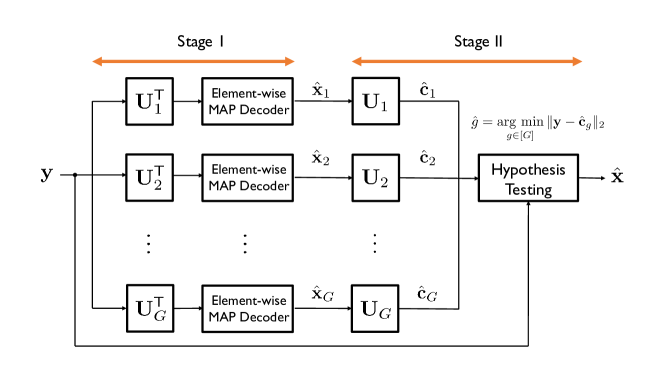
Figure 2: Two-stage MAP decoder for BOSS codes in the AWGN channel.

III Approximate MAP Decoder

This section presents an approximate MAP decoder featuring low decoding latency and complexity. We first explain the motivation of the approximate MAP decoder and present the two-stage decoding algorithm in the sequel.

III-A Two-stage MAP Approximation

Under the premise that a codeword ${\bf c}$ is generated using the $g$th sub-dictionary matrix in ${\bf A}$, the codeword can be written as

$${\bf c}={\bf A}{\bf x}={\bf U}_{g}{\bf x}_{g},$$ (13)

where the sub-message vector ${\bf x}_{g}=\sum_{\ell=1}^{L}{\bf x}_{g}^{(\ell)}$ is a member of the set

$$\mathscr{X}_{g}=\left\{{\bf x}_{g}|{\bf x}_{g}\in\mathcal{A}^{M},\|{\bf x}_{g}\|_{0}=\sum_{\ell=1}^{L}K_{\ell}\right\}.$$ (14)

Let $\mathscr{H}_{g}$ be a hypothesis that the transmitted codeword is constructed with a sub-dictionary matrix $\mathbf{U}_{g}$:

$$\mathscr{H}_{g}:\mathbf{c}=\mathbf{U}_{g}{\bf x}_{g}.$$ (15)

Then, the MAP decoding problem can be decomposed into two different sub-MAP tasks, i.e.,

$$\hat{{\bf x}}^{\text{MAP}} =\underset{{\bf x}\in\mathscr{X}}{\arg\,\max}\,\mathbb{P}({\bf x}|\mathbf{y})$$

$$=\underset{{\bf x}_{g}\in\mathscr{X}_{g},g\in[G]}{\arg\,\max}\,\mathbb{P}({\bf x}_{g},\mathscr{H}_{g}|\mathbf{y})$$

$$=\underset{{\bf x}_{g}\in\mathscr{X}_{g},g\in[G]}{\arg\,\max}\,\mathbb{P}({\bf x}_{g}|\mathbf{y},\mathscr{H}_{g})\mathbb{P}(\mathscr{H}_{g}|\mathbf{y}).{}$$ (16)

Solving this MAP decoding problem requires the complexity order of $\mathcal{O}(|\mathscr{X}|)$, which is prohibitively high as the number of information bits increases. To diminish the decoding complexity, we present a two-stage MAP decoder. The key idea of the two-stage MAP decoder is to solve the MAP decoding problem in (16) independently for ${\bf x}_{g}\in\mathscr{X}_{g}$ and $g\in[G]$, respectively. To be specific, in the first stage, the decoder first identifies ${\bf\hat{x}}_{g}$ under $\mathscr{H}_{g}$

$${\bf\hat{x}}_{g}=\underset{{\bf x}_{g}\in\mathscr{X}_{g}}{\arg\,\max}\,\mathbb{P}({\bf x}_{g}|\mathbf{y},\mathscr{H}_{g}).$$ (17)

Then, in the second stage, using the decoded ${\bf\hat{x}}_{g}$, it finds the block index ${\hat{g}}$:

$${\hat{g}}=\underset{g\in[G]}{\arg\,\max}\,\mathbb{P}(\mathscr{H}_{g}|\mathbf{y}).$$ (18)

III-B Two-stage MAP Decoder

We explain our two-stage MAP decoding algorithm.

Sparse message vector recovery: As illustrated in Fig. 2, in the first stage, the decoder aims at identifying ${\bf x}_{g}$ under each hypothesis $\mathscr{H}_{g}$ in parallel. To this end, the decoder simply takes a fast unitary transform to the received signal vector ${\bf y}$ and produces $G$ transformed receive vectors as

$$\mathbf{y}_{g}=\mathbf{U}_{g}^{\mathsf{T}}\mathbf{y}={\bf x}_{g}+\tilde{\mathbf{v}}_{g},$$ (19)

for $g\in[G]$, and $\tilde{\mathbf{v}}_{g}=\mathbf{U}_{g}^{\mathsf{T}}\mathbf{v}$ follows the identical distribution as $\mathbf{v}$ because the Gaussian distribution is invariant under the unitary transform. The complexity order to obtain ${\bf y}_{g}$ for $g\in[G]$ is $\mathcal{O}(GM\log M)$ thanks to the fast transform for $\mathbf{U}_{g}^{\mathsf{T}}={\bf U}_{1}^{\top}{\bf P}_{g}^{\top}$.

Now, the decoder solves the first sub-MAP decoding problem using $\mathbf{y}_{g}$:

$$\hat{{\bf x}}_{g}=\underset{{\bf x}_{g}\in\mathscr{X}_{g}}{\arg\,\max}\,\mathbb{P}\left({\bf x}_{g}|\mathbf{y},\mathscr{H}_{g}\right)=\underset{{\bf x}_{g}\in\mathscr{X}_{g}}{\arg\,\max}\,\mathbb{P}\left({\bf x}_{g}|\mathbf{y}_{g}\right).$$ (20)

Exploiting the fact that the support of ${\bf x}_{g}$ is a union of mutual-exclusive index sets from $L$ layers, we compute the log of joint a posteriori probability (APP) in (20) and factorizing:

$$\log\mathbb{P}({\bf x}_{g}|\mathbf{y}_{g}) =\sum_{\ell=1}^{L}\log\mathbb{P}({\bf x}_{g}^{(\ell)}|\mathbf{y}_{g},{\bf x}^{(\ell-1)}_{g},\dots,{\bf x}_{g}^{(2)},{\bf x}_{g}^{(1)})$$

$$=\sum_{\ell=1}^{L}\log\mathbb{P}({\bf x}_{g}^{(\ell)}|\mathbf{y}_{g},\mathcal{I}_{g}^{(\ell-1)},\dots,\mathcal{I}_{g}^{(2)},\mathcal{I}_{g}^{(1)}),{}$$ (21)

where the second equality follows from that previous non-zero supports, $\mathcal{I}^{(\ell-1)}_{g},\dots,\mathcal{I}_{g}^{(2)},\mathcal{I}_{g}^{(1)}$, provide sufficient information to decode ${\bf x}_{g}^{(\ell)}$. Hence, the decoder shall leverage side information obtained in the preceding layers to recover ${\bf x}_{g}^{(\ell)}$ and update the conditional likelihoods accordingly. This motivates to design a decoding algorithm based on successive support set cancellation. From the Bayes’s rule as in [32, 37], the $\ell$th layer’s log likelihood in (21) is reformulated as

$$\log\mathbb{P}({\bf x}_{g}^{(\ell)}|\mathbf{y}_{g},\hat{\mathcal{I}}^{(\ell-1)}_{g},\dots,\hat{\mathcal{I}}^{(2)}_{g},\hat{\mathcal{I}}_{g}^{(1)})=\frac{1}{C}\sum_{m\in\hat{\mathscr{M}}_{g}^{(\ell)}}\log\frac{\mathbb{P}(y_{g,m}|x^{(\ell)}_{g,m})\mathbb{P}(x^{(\ell)}_{g,m})}{\mathbb{P}(y_{g,m})}\mathbf{1}_{\{\|{\bf x}_{g}^{(\ell)}\|_{0}=K_{\ell}\}},$$ (22)

where $C\in\mathbb{R}^{+}$ is a normalizing constant, and a candidate set estimate $\hat{\mathscr{M}}^{(\ell)}_{g}$ is defined as

$$\hat{\mathscr{M}}^{(\ell)}_{g}=[M]\backslash\cup_{j=1}^{\ell-1}\hat{\mathcal{I}}_{g}^{(j)}.$$ (23)

Here and hereinafter, we omit support estimates obtained beforehand for notational simplicity in (22), as they are already manifested in $\hat{\mathscr{M}}_{g}^{(\ell)}$. The permissible set in (23) is updated at each iteration so that prior information on previous guesses is properly incorporated into subsequent decoding processes. Note that estimates in (23) may differ by hypothesis $\mathscr{H}_{g}$, but they all feature the same cardinality predefined in encoding:

$$|\hat{\mathscr{M}}^{(\ell)}_{g}|=2^{B_{\ell}}\leq\left(M-\sum_{j=1}^{\ell-1}K_{j}\right),\quad\quad\forall g\in[G].$$ (24)

The element-wise conditional likelihood function in (22) is given by

$$\mathbb{P}\left(y_{g,m}|x^{(\ell)}_{g,m}\right)=\begin{cases}\frac{1}{J_{\ell}}\sum_{j=1}^{J_{\ell}}\frac{1}{\sqrt{2\pi\sigma_{v}^{2}}}e^{-\frac{|y_{g,m}-\alpha_{\ell,j}|^{2}}{2\sigma_{v}^{2}}}&\text{if }\,x^{(\ell)}_{g,m}\in\mathcal{A}_{\ell}\\ \frac{1}{\sqrt{2\pi\sigma_{v}^{2}}}e^{-\frac{|y_{g,m}|^{2}}{2\sigma_{v}^{2}}}&\text{else.}\end{cases}$$ (25)

As values of $\mathcal{A}_{\ell}$ are uniformly allocated to non-zero entries of ${\bf x}^{(\ell)}_{g}$, a prior distribution of $x^{(\ell)}_{g,m}$ is given by

$$\mathbb{P}(x^{(\ell)}_{g,m})=\begin{cases}p^{(\ell)}_{g,m},&\text{if }x^{(\ell)}_{g,m}\in\mathcal{A}_{\ell}\\ 1-p^{(\ell)}_{g,m},&\text{if }x^{(\ell)}_{g,m}=0,\end{cases}$$ (26)

where $p^{(\ell)}_{g,m}$ is the probability of $x^{(\ell)}_{g,m}$ being a non-zero element given by

$$p^{(\ell)}_{g,m}=\frac{K_{\ell}}{|\mathscr{M}^{(\ell)}|}=\frac{K_{\ell}}{M-\sum_{j=1}^{\ell-1}K_{j}}.$$ (27)

Invoking (25) and (26), we have the marginal distribution of $y_{g,m}$:

$$\mathbb{P}(y_{g,m}) =\mathbb{P}(y_{g,m}|x^{(\ell)}_{g,m}\in\mathcal{A}_{\ell})\mathbb{P}(x^{(\ell)}_{g,m}\in\mathcal{A}_{\ell})+\mathbb{P}(y_{g,m}|x^{(\ell)}_{g,m}=0)\mathbb{P}(x^{(\ell)}_{g,m}=0)$$

$$=\frac{1}{J_{\ell}}\sum_{j=1}^{J_{\ell}}\frac{1}{\sqrt{2\pi\sigma_{v}^{2}}}e^{-\frac{|y_{g,m}-\alpha_{\ell,j}|^{2}}{2\sigma_{v}^{2}}}p^{(\ell)}_{g,m}+\frac{1}{\sqrt{2\pi\sigma_{v}^{2}}}e^{-\frac{|y_{g,m}|^{2}}{2\sigma_{v}^{2}}}(1-p^{(\ell)}_{g,m}).{}$$ (28)

Note that recovery of a sparse vector ${\bf x}_{g}^{(\ell)}$ is equivalent to identification of its non-zero element locations such that paired columns of $\mathbf{U}_{g}$ constitute a sub-codeword $\mathbf{c}^{(\ell)}$. For every index $m\in\hat{\mathscr{M}}^{(\ell)}_{g}$, the decoder computes its probability of being an element of $\mathcal{I}^{(\ell)}$, i.e. a likelihood of $x^{(\ell)}_{g,m}$ taking on value from $\mathcal{A}_{\ell}$ conditioned on $y_{g,m}$:

$$\log\mathbb{P}(m\in\mathcal{I}^{(\ell)}|y_{g,m}) =\log\frac{\mathbb{P}(y_{g,m}|x^{(\ell)}_{g,m}\in\mathcal{A}_{\ell})\mathbb{P}(x^{(\ell)}_{g,m}\in\mathcal{A}_{\ell})}{\mathbb{P}(y_{g,m})}$$

$$=\log\frac{\frac{1}{J_{\ell}}\sum_{j=1}^{J_{\ell}}\frac{1}{\sqrt{2\pi\sigma_{v}^{2}}}e^{-\frac{|y_{g,m}-\alpha_{\ell,j}|^{2}}{2\sigma_{v}^{2}}}p^{(\ell)}_{g,m}}{\frac{1}{J_{\ell}}\sum_{j=1}^{J_{\ell}}\frac{1}{\sqrt{2\pi\sigma_{v}^{2}}}e^{-\frac{|y_{g,m}-\alpha_{\ell,j}|^{2}}{2\sigma_{v}^{2}}}p^{(\ell)}_{g,m}+\frac{1}{\sqrt{2\pi\sigma_{v}^{2}}}e^{-\frac{|y_{g,m}|^{2}}{2\sigma_{v}^{2}}}(1-p^{(\ell)}_{g,m})}.{}$$ (29)

The decoder sorts $\hat{\mathscr{M}}^{(\ell)}_{g}$ by the MAP metric in (29), which is monotone increasing with respect to $y_{g,m}$. To satisfy the sparsity requirement $\mathbf{1}_{\{\|{\bf x}^{(\ell)}_{g}\|_{0}=K_{\ell}\}}$ in (22), the decoder selects $K_{\ell}$ indices that have the highest likelihoods and generates an ordered support estimate $\hat{\mathcal{I}}^{(\ell)}_{g}$:

$$\hat{\mathcal{I}}^{(\ell)}_{g}=\left\{\hat{i}^{(\ell)}_{g,1},\hat{i}^{(\ell)}_{g,2},\dots,\hat{i}^{(\ell)}_{g,K_{\ell}}\right\},$$ (30)

where $\mathbb{P}(\hat{i}^{(\ell)}_{g,j}\in\mathcal{I}^{(\ell)}|y_{g,j})\geq\mathbb{P}(\hat{i}^{(\ell)}_{g,k}\in\mathcal{I}^{(\ell)}|y_{g,k})$ for $j<k$. Once the layer support estimate is determined, the decoder performs another MAP estimation to identify the signal levels of $x^{(\ell)}_{g,m}$ for $m\in\hat{\mathcal{I}}_{g}^{(\ell)}$. In particular, this simplifies to the minimum Euclidean distance decoding:

$$\hat{x}^{(\ell)}_{g,m} =\underset{\alpha_{\ell,j}\in\mathcal{A}_{\ell}}{{\arg\,\min}}\,|y_{g,m}-\alpha_{\ell,j}|.{}$$ (31)

After $L$ iterations, we obtain $\hat{{\bf x}}_{g}$ whose support is $\hat{\mathcal{I}}_{g}=\bigcup_{\ell=1}^{L}\hat{\mathcal{I}}_{g}^{(\ell)}$. Fig. 3 describes the first stage under hypothesis $\mathscr{H}_{g}$.

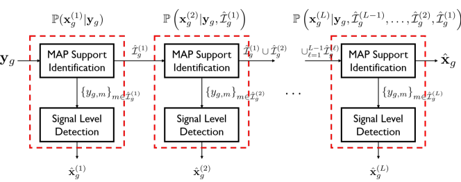
Figure 3: Recovery of a sparse message vector under hypothesis $\mathscr{H}_{g}$.

The block index recovery: Using $\hat{{\bf x}}_{g}$ for $g\in[G]$, in the second stage, the decoder performs the hypothesis testing to identify a true block index $g$. For every $\hat{{\bf x}}_{g}$, the decoder generates a tentative codeword as $\hat{\mathbf{c}}_{g}=\mathbf{U}_{g}\hat{{\bf x}}_{g}$. Since $\mathbf{v}$ is the Gaussian white noise vector, and the encoder has selected the block index uniformly from $[G]$, the second sub-MAP decoding problem is reduced to seeking $\hat{\mathbf{c}}_{g}$ that is closest to $\mathbf{y}$:

$$\hat{g}=\underset{g\in[G]}{\arg\,\max}\,\mathbb{P}(\mathscr{H}_{g}|\mathbf{y})=\underset{g\in[G]}{\arg\,\min}\,\|\mathbf{y}-\hat{\mathbf{c}}_{g}\|_{2}.$$ (32)

As a result, the decoder obtains the estimate of a sparse message vector of dimension $N$ with $K=\sum_{\ell=1}^{L}K_{\ell}$ non-zero entries, all located in the $\hat{g}$th segment, as

$$\hat{{\bf x}}^{\text{MAP}}=\begin{bmatrix}\mathbf{0}_{M}^{\mathsf{T}}&\cdots&{\hat{{\bf x}}_{\hat{g}}}^{\mathsf{T}}&\cdots&\mathbf{0}_{M}^{\mathsf{T}}\end{bmatrix}^{\mathsf{T}}.$$ (33)

Remark 3 (Decoding complexity): The decoding complexity order of the proposed two-stage MAP decoder is sub-quadratic in the blocklength, i.e., $\mathcal{O}(GM\log M)$. Specifically, under the hypothesis of $\mathscr{H}_{g}$, the decoder first computes $\mathbf{y}_{g}$. To accomplish this, the decoder first takes the permutation using ${\bf P}_{g}$ and then performs the fast transform with ${\bf U}_{1}$, i.e., ${\bf U}_{g}^{\top}={\bf U}_{1}^{\top}{\bf P}_{g}^{\top}$. This procedure requires the complexity of $\mathcal{O}(GM\log M)$. The decoder, then, calculates $|\mathscr{M}^{(\ell)}|\leq M-\sum_{j=1}^{\ell-1}K_{j}$ APPs in (29) and selects $K_{\ell}$ indices with the largest APP values to estimate the support. Hence, $\hat{\mathcal{I}}_{g}^{(\ell)}$ can be obtained with the complexity order $\mathcal{O}\left(\left(M-\sum_{j=1}^{\ell-1}K_{j}\right)\log_{2}(K_{\ell})\right)$. After $\hat{\mathcal{I}}_{g}^{(\ell)}$ is found, the decoder performs element-wise maximum likelihood signal level detection for the $\ell$th layer, which takes $J_{\ell}K_{\ell}$ computations. The $G$ sub-message estimates $\hat{{\bf x}}_{g}$ are obtained by repeatedly performing the identical procedures. In the last stage, the decoder generates $G$ codeword candidates and compares their Euclidean distance from $\mathbf{y}$. This re-encoding task, however, makes a negligible contribution to the overall decoding complexity, as each candidate is a linear combination of columns of $\mathbf{U}_{g}$. As a result, the total decoding complexity is $\mathcal{O}\left(GM\log(M)\right)$, which is sub-quadratic in the blocklength.

Remark 4 (Optimality of a simple ordered statistics decoder): We consider a two-layered BOSS code with uniform sparsity $K_{1}=K_{2}$; $\mathcal{A}_{1}=\{1\}$ and $\mathcal{A}_{2}=\{-1\}$; and an arbitrary block size $G$. In this case, we show that the first procedure of the proposed two-stage MAP decoding algorithm is equivalent to a simple ordered statistics (OS) decoder. By plugging

$$\mathbb{P}(y_{g,m}|m\in\mathcal{I}^{(1)})=\frac{1}{\sqrt{2\pi\sigma_{v}^{2}}}\exp\left(-\frac{(y_{g,m}-1)^{2}}{2\sigma_{v}^{2}}\right)$$ (34)

and

$$\mathbb{P}(y_{g,m}|m\notin\mathcal{I}^{(1)})$$

$$=\mathbb{P}(y_{g,m}|m\in\mathcal{I}^{(2)})\mathbb{P}(m\in\mathcal{I}^{(2)})+\mathbb{P}\left(y_{g,m}|m\notin(\mathcal{I}^{(1)}\cup\mathcal{I}^{(2)})\right)\mathbb{P}(m\notin(\mathcal{I}^{(1)}\cup\mathcal{I}^{(2)}))$$

$$=\frac{1}{\sqrt{2\pi\sigma_{v}^{2}}}\exp\left(-\frac{(y_{g,m}+1)^{2}}{2\sigma_{v}^{2}}\right)\frac{K_{1}}{N-K_{1}}+\frac{1}{\sqrt{2\pi\sigma_{v}^{2}}}\exp\left(-\frac{-y_{g,m}^{2}}{2\sigma_{v}^{2}}\right)\frac{N-2K_{1}}{N}{}$$ (35)

into (25), we obtain the log APP of an event $m\in\mathcal{I}^{(1)}$:

$$\log\mathbb{P}(m\in\mathcal{I}^{(1)}|y_{g,m})=\frac{1}{1+\exp\left(-\frac{2y_{g,m}}{\sigma_{v}^{2}}\right)\frac{N}{N-K_{1}}+\exp\left(-\frac{2y_{g,m}-1}{2\sigma_{v}^{2}}\right)\frac{(N-2K_{1})}{K_{1}}}.$$ (36)

$\log\mathbb{P}(m\in\mathcal{I}^{(1)}|y_{g,m})$ is a monotonically increasing function of $y_{g,m}$, so we conclude that the support estimate $\hat{\mathcal{I}}_{g}^{(1)}$ is determined by the $K_{1}$ largest values in $\mathbf{y}_{g}$. Similarly, $\hat{\mathcal{I}}_{g}^{(2)}$ is equivalent to a set of $K_{2}$ smallest entries in $\mathbf{y}_{g}$, except $y_{g,j}$ for $j\in\hat{\mathcal{I}}_{g}^{(1)}$.

This OS decoder is particularly useful for the fast decoding because the sorting algorithm requiring a complexity of $\mathcal{O}(\log(K_{1}+K_{2})M)$ is sufficient to decode ${\bf\hat{x}}_{g}$ from ${\bf y}_{g}$. In our simulations, we shall use this OS decoder for implementation efficiency.

IV Performance Analysis

In this section, we derive an exact analytical expression for the BLERs of single-layered BOSS codes with the proposed two-stage MAP decoding. Our analysis provides an insight into how the BLER changes according to blocklength $M$, the number of unitary matrices $G$, and $\frac{E_{\rm b}}{N_{0}}$. The following theorem is the main result of this section.

Theorem 1. Let $\mathcal{E}_{1}$ and $\mathcal{E}_{2}$ be the error events for the first and second stage decoding. The BLER of a single-layered BOSS code with $\mathcal{A}=\{1\}$ and rate $R=\frac{\lfloor\log_{2}(M)\rfloor+\lfloor\log_{2}(G)\rfloor}{M}$ is given by

$$P_{\sf BLER}(M,G,\sigma_{v}^{2})=\mathbb{P}(\mathcal{E}_{1})+\mathbb{P}(\mathcal{E}_{2}|\mathcal{E}_{1}^{c})\mathbb{P}(\mathcal{E}_{1}^{c}),{}$$ (37)

where

$$\mathbb{P}(\mathcal{E}_{1})=1-\frac{(M-1)}{\sqrt{2\pi\sigma_{v}^{2}}}\int_{-\infty}^{\infty}Q\left(\frac{y-1}{\sigma_{v}}\right)\left[1-Q\left(\frac{y}{\sigma_{v}}\right)\right]^{M-2}e^{-\frac{y^{2}}{2\sigma_{v}^{2}}}{\rm d}y,$$ (38)

and

$$\mathbb{P}(\mathcal{E}_{2}|\mathcal{E}_{1}^{c})=1-\left[\frac{\Gamma\left(\frac{M}{2}\right)}{\sqrt{\pi}\Gamma\left(\frac{M-1}{2}\right)}\int_{-1}^{1}Q\left(\frac{w-1}{\sqrt{2\sigma_{v}^{2}}}\right)(1-w^{2})^{\frac{M-3}{2}}{\rm d}w\right]^{M(G-1)}.$$ (39)

Proof. See Appendix A.

Although the BLER expression in Theorem 1 is integral form, it illuminates how the decoding performance of BOSS codes is affected by code parameters. Note that the noise power $\sigma_{v}^{2}$ is related to $\frac{E_{\rm b}}{N_{0}}$ and code rate $R=\frac{\lfloor\log_{2}(M)\rfloor+\lfloor\log_{2}(G)\rfloor}{M}$ as

$$\sigma_{v}^{2}=\frac{1}{M}\frac{1}{2R\frac{E_{\rm b}}{N_{0}}}=\frac{1}{2(\lfloor\log_{2}(M)\rfloor+\lfloor\log_{2}(G)\rfloor)\frac{E_{\rm b}}{N_{0}}}.$$ (40)

First, for fixed $\frac{E_{\rm b}}{N_{0}}$ and $G$, it is evident that both $\mathbb{P}(\mathcal{E}_{1})$ and $\mathbb{P}(\mathcal{E}_{2})$ decrease as blocklength $M$ increases because the effective noise power $\sigma_{v}^{2}$ is inversely proportional to $M$, and $\mathbb{P}(\mathcal{E}_{1})$ and $\mathbb{P}(\mathcal{E}_{2})$ are decreasing functions with respect to $M$. This confirms our intuition that the BOSS code with a large blocklength can improve the BLER performance. Second, for fixed $M$, increasing the number of unitary blocks $G$ impacts the BLERs differently depending on the noise power $\sigma_{v}^{2}$. When $\frac{E_{\rm b}}{N_{0}}$ is sufficiently high, the second stage decoding error can vanish, i.e., $\lim_{\sigma_{v}^{2}\rightarrow 0}\mathbb{P}(\mathcal{E}_{2}|\mathcal{E}_{1}^{c})\rightarrow 0$. This is somewhat surprising because increasing the code rate by using more $G$ unitary blocks does not occur any second stage decoding error, provided that $\frac{E_{\rm b}}{N_{0}}$ is high enough. In this case, the resultant BLER is bounded by the first stage decoding error. However, when $\frac{E_{\rm b}}{N_{0}}$ is not sufficiently high, increasing $G$ deteriorates the second stage decoding performance. Lastly, for fixed $G$, and $M$, it is apparent that the decoding error approaches zero as increasing $\frac{E_{\rm b}}{N_{0}}$. This also confirms that our BOSS code with the two-stage decoder does not have error-floor effects, which is particularly useful for URLLC applications such as telesurgery and augmented reality wherein accurate, haptic feedback is required, so a target BLER is extremely low (e.g., $10^{-6}$).

V CA-BOSS Codes

In this section, we present a serially concatenated scheme of BOSS codes with short CRC as the outer code. This new family of BOSS codes, namely CA-BOSS codes, further improves the decoding performance with a simple list decoder, while increasing the decoding complexity very marginally.

V-A Concatenated Encoding

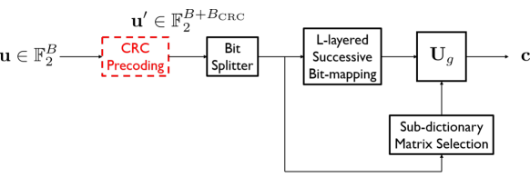
Figure 4: Concatenated encoding of CA-BOSS codes.

In the proposed MAP-based decoding algorithm, wrong decisions made in the early phases of the first stage cannot be fixed and result in incorrect candidate sets for the remaining layers. We adopt CRC precoding to help the decoder determine the non-zero support. $B_{\text{CRC}}$ CRC bits are added to the data block $\mathbf{u}\in\mathbb{F}_{2}^{B}$. The appended block $\mathbf{u}^{\prime}\in\mathbb{F}_{2}^{B+B_{\text{CRC}}}$ is then fed into the original BOSS encoder, and its fractions are sequentially mapped into a dictionary block index and non-zero elements. The CA-BOSS encoder is illustrated in Fig. 4 with a block newly added to the original BOSS encoder colored red.

V-B List Decoder

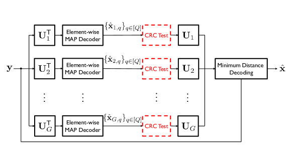
Figure 5: The MAP-List decoder design of CA-BOSS codes.

We introduce a list decoding algorithm based on the two-stage MAP decoder to take advantage of CRC error-detection. Under each $\mathscr{H}_{g}$, the decoder finds $Q$ sub-message vector estimates, i.e., $\left\{\hat{\mathbf{x}}_{g,1},\hat{\mathbf{x}}_{g,2},\dots,\hat{\mathbf{x}}_{g,Q}\right\}$. The list can be generated in various ways. For example, when a two-layered BOSS code with $K_{1}=K_{2}=1$ is evaluated, the decoder can select the two most likely indices at each layer and obtain a list of $Q=4$, using their combinations. The decoder inverse-maps each provisional support $\{\hat{\mathcal{I}}_{g,q}\}_{q\in[Q]}$ and $g$ to a bit sequence and performs a CRC test to identify a valid combination of the block and non-zero indices. Only surviving message vector estimates are transferred to the next decoding stage and re-encoded into tentative codewords. Finally, the decoder determines the block index and most probable valid support by choosing the codeword candidate closest to $\mathbf{y}$. The proposed MAP-List decoding is described in Fig. 5.

VI Numerical Results

In this section, we provide simulation results to validate the error-correcting performance of proposed BOSS codes under the two-stage MAP decoding algorithm. We then investigate how CRC concatenation affects the performance of BOSS codes.

VI-A BLER Comparison in the AWGN Channel

We adopt BLER versus $E_{\rm b}/N_{\rm 0}$ as an assessment of the two-stage MAP decoder in the AWGN channel to take into consideration low code rates and non-standard modulation techniques of BOSS codes.

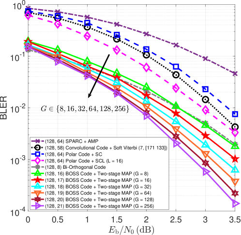
Figure 6: BLER comparison with existing codes.

BOSS codes: We simulated two-layered BOSS codes with blocklength $M=128$; symmetric sparsity $K_{1}=K_{2}=1$; singleton PAM alphabets $\mathcal{A}_{1}=\{1\}$ and $\mathcal{A}_{2}=\{-1\}$; and various block sizes. For $G=16$, the code rate is $\frac{17}{128}\approx 0.13$.

Polar codes: We considered a $1/2$ rate polar code of length $128$, using the binary phase-shift keying (BPSK) modulation. The code construction is based on the $2\times 2$ Arıkan kernel, and the 3GPP 5G NR frozen set, i.e., pre-computed SNR-independent channel reliability order, [38] is adopted. SC and SCL decoding algorithm with search width $L=16$ were employed.

Convolutional codes: A convolutional code of length $128$ with BPSK modulation was evaluated under the soft Viterbi algorithm. The generator polynomials are $\textsl{g}=[171\,133]$ in octal notation, so the constraint length is $7$. Taking account of rate loss entailed by termination bits, the effective code rate is $\frac{58}{128}\approx 0.45$.

SPARC codes: We used a fat random Gaussian dictionary matrix $\mathbf{A}$ consisted of $8$ sections to generate a SPARC of length $128$. Each section contains $256$ columns, i.e., $\mathbf{A}\in\mathbb{R}^{128\times 2048}$, so the code rate is $\frac{8\log_{2}256}{128}=\frac{1}{2}$.

Bi-orthogonal codes: We considered a bi-orthogonal code of length $128$ with a dictionary matrix $\mathbf{A}=[\mathbf{H}_{2^{7}},-\mathbf{H}_{2^{7}}],$ where $\mathbf{H}_{2^{k}}$ is a Hadamard matrix of order $2^{k}$. Each codeword conveys $\log_{2}(2\times 128)=8$ bits in $128$ channel uses.

Fig. 6 shows that BOSS codes outperform polar codes under SCL decoding by a considerable margin: the proposed decoder results in approximately $0.4$ coding gains at BLER of $10^{-4}$ even for $G=8$. The results in Fig. 6 also illustrate a prominent feature of BOSS codes: enlarging the dictionary matrix improves decoding performance at the cost of computational complexity. This trend can be ascribed to an increase in the code rate caused by concatenating the dictionary matrix with more blocks, whereas the average transmit energy $E_{s}$ is preserved. Therefore, the block number parameter $G$ can be appropriately tuned to achieve a desired trade-off between performance and complexity. Surprisingly, no performance saturation was observed when increasing $G$ up to 256. A bi-orthogonal code shows comparable performance to that of our BOSS codes with a few blocks. Therefore, it can be thought as a special case of BOSS codes when $G=2$ and $K=1$.

VI-B Decoding Performance of CA-BOSS codes

Figure 7: BLER performance comparison between CA-BOSS and CA-polar codes.

Fig. 7 compares CA-BOSS codes to the state-of-the-art CA-polar codes under SCL decoding with different search width. It can be seen that CA-BOSS codes outperform ordinary BOSS codes of the same rate by a meaningful margin. Moreover, at high SNR, the CA-BOSS code with $G=128$ even shows superior decoding performance to the BOSS code with $G=256$. We observed from the AWGN simulation result that the performance-complexity trade-off of BOSS coding is controlled by $G$. This favorable trait, however, does not lend itself to CA-BOSS codes, since the effective code rate remains the same. If the list decoding is adopted without CRC concatenation, the decoder at the second stage will generate $Q$ codeword candidates per hypothesis, and incorrect estimates happen to be closer to the observation. The CRC test is capable of ruling out error events caused by invalid support estimates under the true hypothesis. Consequetly, CA-BOSS codes enjoy two gains in reducing decoding complexity by the codeword pruning and enhancing the decoding performance by error detection.

In the low SNR regime, CA-BOSS codes show excellent decoding performance; however, as the SNR increases, BLER of CA-polar codes drops with a precipitous slope, beating CA-BOSS codes.

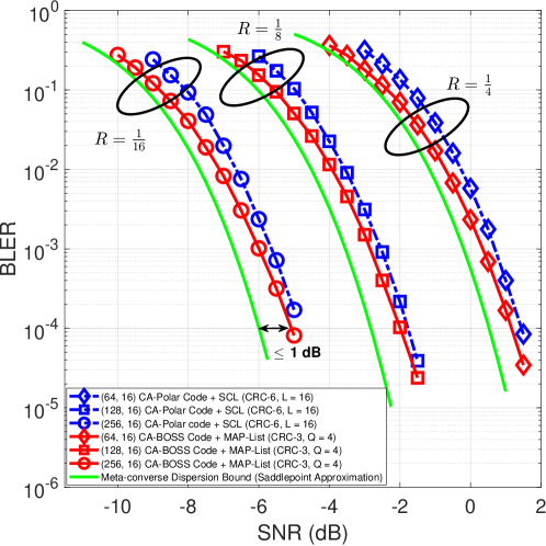
Figure 8: BLER performance comparison for BOSS and polar codes when $R\in\{1/4,1/8,1/16\}$.

Fig. 8 compares CA-BOSS codes with CA-polar codes of the same rate. It turns out that CA-BOSS codes outperform the polar counterparts at every blocklength under consideration, even when attached with the shorter, i.e., weaker, CRC outer code. This remarkable result attests to the error-correction capability of our codes. When transmitting the same information block size, adding CRC bits causes the polar encoder to use additional non-extremal (having mediocre reliability) virtual bit-channels. As a result, the receiver is more prone to errors in the early phase of sequential decoding. This fact, however, is not a concern of CA-BOSS coding.

Fig. 8 also plots the saddlepoint approximation [39] to the meta-converse bound [15]:

$$\eta(n,M)\overset{\triangle}{=}\underset{P^{n}}{\min}\,\underset{Q^{n}}{\max}\{\alpha_{\frac{1}{M}}(P^{n}\times W^{n},P^{n}\times Q^{n})\},$$ (41)

where $M$ is the number of symbols transmitted over a length-$n$ $W^{n}(\cdot|\cdot)$ channel, and $\alpha_{\beta}(P,Q)$ is the smallest type-I error probability across all tests between an input distribution $P$ and auxiliary output distribution $Q$, with a type-II error probability of at most $\beta$. It can be seen that our CA-BOSS codes perform within one dB away from the finite-length channel capacity bounds in all SNRs and rates.

VI-C Validation of BLER Analysis

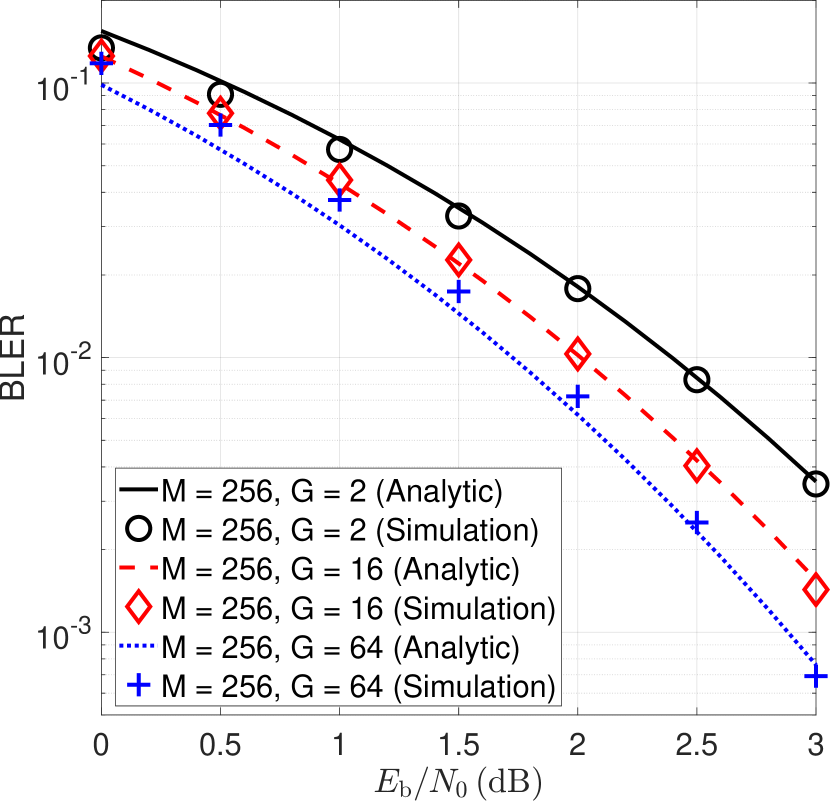
(a)

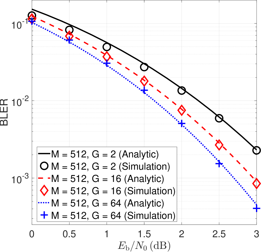
(b)

Figure 9: BLER comparison between analytical and simulation results for $M\in\{256,512\}$ and $G\in\{2,16,64\}$.

Fig. 9 compares the analytical BLER derived in Theorem 1 with the simulations for $M=\{256,512\}$, $\mathcal{A}=\{1\}$, and $G=\{2,16,64\}$. As can be seen, our analytical expression tightly matches with the simulation results for various code parameters, which confirms the exactness of our analysis. In the low $E_{b}/N_{0}$ regime, our analytical results show a small discrepancy with simulations. This gap arises from the numerical precision errors in computing $M(G-1)$ power in (39), and it becomes pronounced as $M(G-1)$ increases. Nonetheless, this gap readily vanishes as $E_{b}/N_{0}$ increases.

VII Conclusion

From the point of view of coded modulation techniques, this work has provided a new type of joint coded modulation method called BOSS codes for URLLC. In particular, we have presented a novel successive encoding technique to generate zero-RIP codewords that are a sparse linear combination of orthogonal columns of a dictionary matrix. A very fast yet noise-tolerant MAP-based decoding algorithm has been proposed for BOSS codes. This two-stage MAP decoder exploits the orthogonality and performs element-wise MAP decoding to identify non-zero coefficients in a parallel structure, thereby achieving near-ML decoding performance with low decoding latency. We then provide the exact BLER expression for single-layered BOSS codes. This analytical formula is useful in understanding on how crucial code parameters affect the performance of BOSS codes. We have further improved the performance of BOSS codes through concatenation with a CRC outer code and shown that CA-BOSS codes achieve the meta-converse bound within one dB in the low code-rate regime.

In recent follow-up work, a robust decoding algorithm for BOSS codes was studied in multi-path fading environments, and the real-time demonstration using NI-PXI according to IEEE 802.11 standards was shown to considerably outperform CA-polar codes with SCL decoding when a codeword transmission experiences multiple fading states [40, 41]. A promising direction for future work is to develop a joint equalizer and decoder that is robust for the multi-fading states. It is also an interesting direction to expand BOSS codes by incorporating phase shift keying modulation in complex AWGN channels to deliver more information bits in an energy-efficient manner.

Appendix

VII-A Proof of Theorem 1

Before providing the proof, we first introduce two lemmas, which are necessary for our proof. The first lemma provides probability distribution of the maximum and minimum of $M$ IID random variables.

Lemma 1. Let $\{X_{m}\}_{m=1}^{M}$ be a sequence of $M$ IID random variables, each with probability density function (PDF) $f_{X}(x)$ and cumulative density function (CDF) $F_{X}(x)$. We also denote the maximum and minimum of the sequence by $X_{\text{max}}=\underset{1\leq m\leq M}{\max}\,X_{m}$ and $X_{\text{min}}=\underset{1\leq m\leq M}{\min}\,X_{m}$ , respectively. Then, the PDF’s of $X_{\text{max}}$ and $X_{\text{min}}$ are

$$f_{X_{\text{max}}}(x) =Mf_{X}(x)F_{X}(x)^{M-1}\quad\text{and}$$ (42)

$$f_{X_{\text{min}}}(x) =Mf_{X}(x)[1-F_{X}(x)]^{M-1}.$$ (43)

Proof. Due to independence, the CDF of $X_{\text{max}}$ can be readily found:

$$F_{X_{\text{max}}}(x)=\prod_{m=1}^{M}\mathbb{P}(X_{m}\leq x)=F_{X}(x)^{M}.$$ (44)

By differentiating $F_{X_{\text{max}}}(x)$ with respect to $x$, we obtain $f_{X_{\text{max}}}(x)$. Similarly, $F_{X_{\text{min}}(x)}=1-\left[1-F_{X}(x)\right]^{M}$, and the rest of the proof is straightforward.

The second lemma provides statistics of an inner product of two IID random unit vectors in an $(M-1)$-dimensional sphere.

Lemma 2. For two random unit-norm vectors, $\mathbf{u}\in\mathbb{R}^{M}$ and $\mathbf{v}\in\mathbb{R}^{M}$, that are uniformly distributed on a sphere $\mathcal{S}^{M-1}$, their inner product $W=\langle\mathbf{u},\mathbf{v}\rangle$ has a PDF given by

$$f_{W}(w)=\frac{\Gamma\left(\frac{M}{2}\right)}{\sqrt{\pi}\Gamma\left(\frac{M-1}{2}\right)}(1-w^{2})^{\frac{M-3}{2}}.$$ (45)

Proof. If $\mathbf{X}=\{X_{1},X_{2},\dots X_{M}\}$ follows the standard multivariate normal distribution, i.e., $X_{i}\sim\mathcal{N}(0,1)$, then $\frac{\mathbf{X}}{\|\mathbf{X}\|_{2}}$ is uniformly distributed on the unit sphere. We assume that $\mathbf{v}=[1,0,\dots,0]$ thanks to spherical symmetry, and then the distribution of $W$ is identical to that of

$$\frac{X_{1}}{\sqrt{X_{1}^{2}+X_{2}^{2}+\cdots+X_{M}^{2}}}.$$ (46)

It is well known that the square of ratio distribution in (46) follows $\text{Beta}(\frac{1}{2},\frac{M-1}{2})$. The rest of the proof is trivial.

Now, we are ready to prove Theorem 1. We denote by $\mathcal{E}_{1}$ and $\mathcal{E}_{2}$ an error event at stage 1 and 2 of the proposed two-stage MAP decoder, respectively. Using these error events, the probability of decoding error is given by

$$\mathbb{P}(\mathcal{E})=\mathbb{P}(\mathcal{E}_{1})+\mathbb{P}(\mathcal{E}_{2}|\mathcal{E}_{1}^{c})\mathbb{P}(\mathcal{E}_{1}^{c}).$$ (47)

We consider a randomly constructed dictionary matrix $\mathbf{A}=\left[\mathbf{U}_{1},\mathbf{U}_{2},\dots,\mathbf{U}_{G}\right]$, i.e., $\mathbf{U}_{i}$ and $\mathbf{U}_{j}$ are independent for $i\neq j\in[G]$. Without loss of generality, we assume that $K_{1}=1$ and $\mathbf{U}_{1}$ has participated in encoding, so $\mathbf{A}\mathbf{x}=\mathbf{U}_{1}\mathbf{x}_{1}$, where $\|\mathbf{x}_{1}\|_{0}=1$. For the AWGN channel, the received symbol in the $m$th channel use is given by

$$Y_{m}=\begin{cases}1+V_{m}&\text{for }m\in\mathcal{I}\\ V_{m}&\text{for }m\notin\mathcal{I},\end{cases}$$ (48)

where $V_{m}$ is a zero-mean Gaussian noise with variance $\sigma_{v}^{2}$. As explained in Remark 4, a simple OS decoder is optimal in this case. Then, the error event at stage is $\{\hat{\mathbf{x}}_{1}\neq\mathbf{x}_{1}\}$, and its probability can be computed as

$$\mathbb{P}(\mathcal{E}_{1}) =1-\mathbb{P}(\mathcal{E}_{1}^{c})$$

$$=1-\mathbb{P}(Y_{\mathcal{I}}^{\text{min}}>Y_{\mathcal{I}^{c}}^{\text{max}}),{}$$ (49)

where $Y_{\mathcal{I}}^{\text{min}}\overset{\triangle}{=}\underset{m\in\mathcal{I}}{\min}\,Y_{m}$ and $Y_{\mathcal{I}^{c}}^{\text{max}}\overset{\triangle}{=}\underset{m\in\mathcal{I}^{c}}{\max}\,Y_{m}$. The conditional expectation theorem gives

$$\mathbb{P}(Y_{\mathcal{I}}^{\text{min}}>Y_{\mathcal{I}^{c}}^{\text{max}}) =\mathbb{E}_{Y_{\mathcal{I}^{c}}^{\text{max}}}\left\{\mathbb{P}(Y_{\mathcal{I}}^{\text{min}}>y)|Y_{\mathcal{I}^{c}}^{\text{max}}=y\right\}$$

$$=\int_{-\infty}^{\infty}\mathbb{P}(Y_{\mathcal{I}}^{\text{min}}>y)f_{Y_{\mathcal{I}^{c}}^{\text{max}}}(y){\rm d}y$$

$$=\int_{-\infty}^{\infty}\mathbb{P}(Y_{\mathcal{I}}^{\text{min}}>y)(M-1)f_{Y_{\mathcal{I}^{c}}}(y)F_{Y_{\mathcal{I}^{c}}}(y)^{M-2}{\rm d}y$$

$$=\frac{(M-1)}{\sqrt{2\pi\sigma_{v}^{2}}}\int_{-\infty}^{\infty}[1-F_{Y_{\mathcal{I}}}(y)]F_{Y_{\mathcal{I}^{c}}}(y)^{M-2}e^{-\frac{y^{2}}{2\sigma_{v}^{2}}}{\rm d}y.{}$$ (50)

Note that $Y_{m}$ is distributed as $\mathcal{N}(1,\sigma_{v}^{2})$ for $m\in\mathcal{I}$ and $\mathcal{N}(0,\sigma_{v}^{2})$ for $m\in\mathcal{I}^{c}$. Plugging $F_{Y_{\mathbb{I}}}(y)=1-Q\left(\frac{y-1}{\sigma_{v}}\right)$ and $F_{Y_{\mathcal{I}^{c}}}(y)=1-Q\left(\frac{y}{\sigma_{v}}\right)$ into (50), we arrive at the expression in (38).

Now, we shift our focus to the second stage. Under the condition that the decoder has correctly estimated a sparse sub-message vector under $\mathscr{H}_{1}$, i.e., $\hat{\mathbf{x}}_{1}=\mathbf{x}_{1}$, an error occurs when at least one codeword estimate $\mathbf{U}_{g}\hat{\mathbf{x}}_{g}$ for $g\in[G]\backslash\{1\}$ is closer to $\mathbf{y}$ in terms of Euclidean distance compared to $\mathbf{U}_{1}\hat{\mathbf{x}}_{1}$. The conditional error probability at stage 2 can be expressed as follows:

$$\mathbb{P}(\mathcal{E}_{2}|\mathcal{E}_{1}^{c}) =1-\mathbb{P}(\hat{g}=1|\hat{\mathbf{x}}_{1}=\mathbf{x}_{1})$$

$$=1-\mathbb{P}\left(\cap_{g\in[G]\backslash\{1\}}\{\mathbf{y}^{\mathsf{T}}\mathbf{U}_{1}\mathbf{x}_{1}>\mathbf{y}^{\mathsf{T}}\mathbf{U}_{g}\hat{\mathbf{x}}_{g}\}\right).{}$$ (51)

We first consider the probability that $\mathbf{y}^{\mathsf{T}}\mathbf{U}_{1}\mathbf{x}_{1}$ is larger than $\mathbf{y}^{\mathsf{T}}\mathbf{U}_{g}\hat{\mathbf{x}}_{g}$. Recall that the OS decoder estimates the support under $\mathscr{H}_{g}$ by finding the maximum element of $\mathbf{U}_{g}^{\mathsf{T}}\mathbf{y}=\mathbf{U}_{g}^{\mathsf{T}}(\mathbf{U}_{1}\mathbf{x}_{1}+\mathbf{v})$. We define the $m$th element of random vector $\mathbf{U}_{g}^{\mathsf{T}}\mathbf{y}$ as

$$\tilde{Y}_{g,m}=\mathbf{u}_{g,m}^{\mathsf{T}}\mathbf{v}+\mathbf{u}_{g,m}^{\mathsf{T}}\mathbf{U}_{1}\mathbf{x}_{1}.$$ (52)

The first term $\tilde{V}_{g,m}=\mathbf{u}_{g,m}^{\mathsf{T}}\mathbf{v}$ is a zero-mean Gaussian random variable with variance $\sigma_{v}^{2}$, while the second term $W_{g,m}=\mathbf{u}_{g,m}^{\mathsf{T}}\mathbf{U}_{1}\mathbf{x}_{1}$ is distributed per Lemma 2. The decoder finds the maximum index:

$$\hat{\mathcal{I}}_{g}=\underset{m\in[M]}{\arg\,\max}\,\mathbf{u}_{g,m}^{\mathsf{T}}\mathbf{U}_{1}\mathbf{x}_{1}+\mathbf{u}_{g,m}^{\mathsf{T}}\mathbf{v}.$$ (53)

The decoder generates $\hat{\mathbf{x}}_{g}$ as a one-hot vector with a non-zero value at $\hat{\mathcal{I}}_{g}$. Therefore, $\mathbf{y}^{\mathsf{T}}\mathbf{U}_{g}\hat{\mathbf{x}}_{g}$ is distributed as the maximum of $\tilde{Y}_{g,m}$, i.e., $\max\,\left\{\tilde{Y}_{g,1},\dots,\tilde{Y}_{g,M}\right\}$, and (51) can be re-written as

$$\mathbb{P}(\mathcal{E}_{2}|\mathcal{E}_{1}^{c}) =1-\mathbb{P}\left(\bigcap_{g\in[G]\backslash\{1\}}\left\{\mathbf{y}^{\mathsf{T}}\mathbf{U}_{1}\mathbf{x}_{1}>\max\left\{\tilde{Y}_{g,1},\dots,\tilde{Y}_{g,M}\right\}\right\}\right)$$

$$=1-\mathbb{P}\left(\bigcap_{\begin{subarray}{c}g\in[G]\backslash\{1\}\\ m\in[M]\end{subarray}}\left\{\mathbf{v}^{\mathsf{T}}\mathbf{U}_{1}\mathbf{x}_{1}+\|\mathbf{U}_{1}\mathbf{x}_{1}\|_{2}^{2}>\tilde{V}_{g,m}+W_{g,m}\right\}\right).{}$$ (54)

Note that $\tilde{Y}_{g,m}=\tilde{V}_{g,m}+W_{g,m}$ is IID for $g\in[G]\backslash\{1\}$. Denoting $\tilde{Z}_{g,m}=\mathbf{v}^{\mathsf{T}}\mathbf{U}_{1}\mathbf{x}_{1}-\tilde{V}_{g,m}$, a zero-mean Gaussian with variance $2\sigma_{v}^{2}$, we obtain the following expression:

$$\mathbb{P}(\mathcal{E}_{2}|\mathcal{E}_{1}^{c}) =1-\prod_{\begin{subarray}{c}g\in[G]\backslash\{1\}\\ m\in[M]\end{subarray}}\mathbb{P}(\tilde{Z}_{g,m}>W_{g,m}-1)$$

$$=1-\prod_{\begin{subarray}{c}g\in[G]\backslash\{1\}\\ m\in[M]\end{subarray}}\mathbb{E}_{W_{g,m}}\left\{\mathbb{P}(\tilde{Z}_{g,m}>w-1)|W_{g,m}=w\right\}$$

$$=1-\left[\frac{\Gamma\left(\frac{M}{2}\right)}{\sqrt{\pi}\Gamma\left(\frac{M-1}{2}\right)}\int_{-1}^{1}Q\left(\frac{w-1}{\sqrt{2\sigma_{v}^{2}}}\right)(1-w^{2})^{\frac{M-3}{2}}{\rm d}w\right]^{M(G-1)}.{}$$ (55)

Finally, by plugging (38) and (55) into (47), we complete the proof.

References

- [1] J. Park, J. Choi, W. Shin, and N. Lee, “Block orthogonal sparse superposition codes,” in IEEE Global Communications Conference (GLOBECOM), 2021, pp. 1–5.
- [2] F. Boccardi, R. W. Heath, A. Lozano, T. L. Marzetta, and P. Popovski, “Five disruptive technology directions for 5G,” IEEE Communications Magazine, vol. 52, no. 2, pp. 74–80, 2014.
- [3] G. P. Fettweis, “The tactile internet: Applications and challenges,” IEEE Vehicular Technology Magazine, vol. 9, no. 1, pp. 64–70, 2014.
- [4] G. Durisi, T. Koch, and P. Popovski, “Toward massive, ultrareliable, and low-latency wireless communication with short packets,” Proceedings of the IEEE, vol. 104, no. 9, pp. 1711–1726, 2016.
- [5] P. Popovski, J. J. Nielsen, C. Stefanovic, E. d. Carvalho, E. Strom, K. F. Trillingsgaard, A.-S. Bana, D. M. Kim, R. Kotaba, J. Park, and R. B. Sorensen, “Wireless access for ultra-reliable low-latency communication: Principles and building blocks,” IEEE Network, vol. 32, no. 2, pp. 16–23, 2018.
- [6] H. Chen, R. Abbas, P. Cheng, M. Shirvanimoghaddam, W. Hardjawana, W. Bao, Y. Li, and B. Vucetic, “Ultra-reliable low latency cellular networks: Use cases, challenges and approaches,” IEEE Communications Magazine, vol. 56, no. 12, pp. 119–125, 2018.
- [7] M. Luvisotto, Z. Pang, and D. Dzung, “Ultra high performance wireless control for critical applications: Challenges and directions,” IEEE Transactions on Industrial Informatics, vol. 13, no. 3, pp. 1448–1459, 2017.
- [8] P. Schulz, M. Matthe, H. Klessig, M. Simsek, G. Fettweis, J. Ansari, S. A. Ashraf, B. Almeroth, J. Voigt, I. Riedel, A. Puschmann, A. Mitschele-Thiel, M. Muller, T. Elste, and M. Windisch, “Latency critical iot applications in 5G: Perspective on the design of radio interface and network architecture,” IEEE Communications Magazine, vol. 55, no. 2, pp. 70–78, 2017.
- [9] M. Sybis, K. Wesolowski, K. Jayasinghe, V. Venkatasubramanian, and V. Vukadinovic, “Channel coding for ultra-reliable low-latency communication in 5G systems,” in IEEE 84th Vehicular Technology Conference (VTC-Fall), 2016, pp. 1–5.
- [10] M. Shirvanimoghaddam, M. S. Mohammadi, R. Abbas, A. Minja, C. Yue, B. Matuz, G. Han, Z. Lin, W. Liu, Y. Li, S. Johnson, and B. Vucetic, “Short block-length codes for ultra-reliable low latency communications,” IEEE Communications Magazine, vol. 57, no. 2, pp. 130–137, 2019.
- [11] C. Berrou, A. Glavieux, and P. Thitimajshima, “Near shannon limit error-correcting coding and decoding: Turbo-codes. 1,” in IEEE International Conference on Communications, vol. 2, 1993, pp. 1064–1070 vol.2.
- [12] R. Gallager, “Low-density parity-check codes,” IRE Transactions on Information Theory, vol. 8, no. 1, pp. 21–28, 1962.
- [13] D. MacKay, “Good error-correcting codes based on very sparse matrices,” IEEE Transactions on Information Theory, vol. 45, no. 2, pp. 399–431, 1999.
- [14] R. Ratasuk, N. Mangalvedhe, Y. Zhang, M. Robert, and J.-P. Koskinen, “Overview of narrowband IoT in LTE Rel-13,” in 2016 IEEE Conference on Standards for Communications and Networking (CSCN), 2016, pp. 1–7.
- [15] Y. Polyanskiy, H. V. Poor, and S. Verdú, “Channel coding rate in the finite blocklength regime,” IEEE Transactions on Information Theory, vol. 56, no. 5, pp. 2307–2359, 2010.
- [16] E. Arıkan, “Channel polarization: A method for constructing capacity-achieving codes for symmetric binary-input memoryless channels,” IEEE Transactions on Information Theory, vol. 55, no. 7, pp. 3051–3073, 2009.
- [17] ——, “From sequential decoding to channel polarization and back again,” arXiv preprint arXiv:1908.09594, 2019.
- [18] I. Tal and A. Vardy, “List decoding of polar codes,” in IEEE International Symposium on Information Theory Proceedings, 2011, pp. 1–5.
- [19] A. Joseph and A. R. Barron, “Least squares superposition codes of moderate dictionary size are reliable at rates up to capacity,” IEEE Transactions on Information Theory, vol. 58, no. 5, pp. 2541–2557, 2012.
- [20] G. Forney and G. Ungerboeck, “Modulation and coding for linear Gaussian channels,” IEEE Transactions on Information Theory, vol. 44, no. 6, pp. 2384–2415, 1998.
- [21] G. Caire, G. Taricco, and E. Biglieri, “Bit-interleaved coded modulation,” IEEE Transactions on Information Theory, vol. 44, no. 3, pp. 927–946, 1998.
- [22] A. Joseph and A. R. Barron, “Fast sparse superposition codes have near exponential error probability for ,” IEEE Transactions on Information Theory, vol. 60, no. 2, pp. 919–942, 2014.
- [23] C. Sanghee and A. Barron, “Approximate iterative bayes optimal estimates for high-rate sparse superposition codes,” in Sixth Workshop on Information-Theoretic Methods in Science and Engineering, 2013.
- [24] A. Greig and R. Venkataramanan, “Techniques for improving the finite length performance of sparse superposition codes,” IEEE Transactions on Communications, vol. 66, no. 3, pp. 905–917, 2018.
- [25] J. Barbier and F. Krzakala, “Approximate message-passing decoder and capacity achieving sparse superposition codes,” IEEE Transactions on Information Theory, vol. 63, no. 8, pp. 4894–4927, 2017.
- [26] C. Rush, A. Greig, and R. Venkataramanan, “Capacity-achieving sparse superposition codes via approximate message passing decoding,” IEEE Transactions on Information Theory, vol. 63, no. 3, pp. 1476–1500, 2017.
- [27] E. Candès, J. Romberg, and T. Tao, “Robust uncertainty principles: exact signal reconstruction from highly incomplete frequency information,” IEEE Transactions on Information Theory, vol. 52, no. 2, pp. 489–509, 2006.
- [28] D. L. Donoho, A. Maleki, and A. Montanari, “Message-passing algorithms for compressed sensing,” Proceedings of the National Academy of Sciences, vol. 106, no. 45, pp. 18 914–18 919, 2009.
- [29] E. J. Candès, “The restricted isometry property and its implications for compressed sensing,” Comptes Rendus Mathematique, vol. 346, no. 9, pp. 589–592, 2008. [Online]. Available: https://www.sciencedirect.com/science/article/pii/S1631073X08000964
- [30] R. Calderbank, S. Howard, and S. Jafarpour, “Construction of a large class of deterministic sensing matrices that satisfy a statistical isometry property,” IEEE Journal of Selected Topics in Signal Processing, vol. 4, no. 2, pp. 358–374, 2010.
- [31] A. G. Perotti and B. M. Popovic, “Quasi-orthogonal sparse superposition codes,” in IEEE Global Communications Conference (GLOBECOM), 2019, pp. 1–6.
- [32] Y. Nam and N. Lee, “Bayesian matching pursuit: A finite-alphabet sparse signal recovery algorithm for quantized compressive sensing,” IEEE Signal Processing Letters, vol. 26, no. 9, pp. 1285–1289, 2019.
- [33] E. Candès and T. Tao, “Decoding by linear programming,” IEEE Transactions on Information Theory, vol. 51, no. 12, pp. 4203–4215, 2005.
- [34] E. Başar, U. Aygölü, E. Panayırcı, and H. V. Poor, “Orthogonal frequency division multiplexing with index modulation,” IEEE Transactions on Signal Processing, vol. 61, no. 22, pp. 5536–5549, 2013.
- [35] M. D. Renzo, H. Haas, and P. M. Grant, “Spatial modulation for multiple-antenna wireless systems: a survey,” IEEE Communications Magazine, vol. 49, no. 12, pp. 182–191, 2011.
- [36] J. Choi, Y. Nam, and N. Lee, “Spatial lattice modulation for MIMO systems,” IEEE Transactions on Signal Processing, vol. 66, no. 12, pp. 3185–3198, 2018.
- [37] N. Lee, “MAP support detection for greedy sparse signal recovery algorithms in compressive sensing,” IEEE Transactions on Signal Processing, vol. 64, no. 19, pp. 4987–4999, 2016.
- [38] 3rd Generation Partnership Project; Technical Specification Group Radio Access network; NR; Multiplexing and Channel Coding, Release 16, V16.2.0, 3GPP Standard TS 38.212, July. 2020.
- [39] G. Vazquez-Vilar, A. G. Fabregas, T. Koch, and A. Lancho, “Saddlepoint approximation of the error probability of binary hypothesis testing,” in IEEE International Symposium on Information Theory (ISIT), 2018, pp. 2306–2310.
- [40] D. Han, B. Lee, S. Lee, and N. Lee, “Mmse-a-map decoder for block orthogonal sparse superposition codes in fading channels,” in ICC 2022 - IEEE International Conference on Communications, 2022, pp. 2477–2482.
- [41] B. Lee, D. Han, and N. Lee, “Demo: Real-time implementation of block orthogonal sparse superposition codes,” in IEEE International Conference on Communications, 2022.