Marco Gramatica
School of Mathematical Sciences, Queen Mary University of London, London, UK
Silvia Liverani
School of Mathematical Sciences, Queen Mary University of London, London, UK
The Alan Turing Institute, The British Library, London, UK
Peter Congdon
School of Geography, Queen Mary University of London, London, UK
1 Proofs of main results
Corollary 1.
Let be as defined in M1-M3, then iff , can be expressed as the covariance matrix of a CAR model for a unique pair of matrices and .
Proof.
To prove the sufficiency part, since Theorem 2.1 states that the statement is true for any positive-definite covariance matrix, we only need to prove that is in fact positive definite. This can be achieved by simply noting that: and both and are of full rank, so by applying (3) in Theorem 14.2.9 by [harville2008matrix] we obtain the positive definiteness of .
To prove necessity, we observe that when making it rank deficient, thus we conclude that it cannot be also positive definite.
∎
Lemma 1.
Let be a matrix as defined in M1-M3. has a left inverse iff , and this matrix is unique iff .
Proof.
In the case it is obvious that exists, given that is of full rank by M3, and in fact coincides with guaranteeing uniqueness.
Since an matrix has a left inverse iff it is of full column rank, it follows that when , will not have any such inverse.
Moving on to the case, following Theorem 9.2.7 in [harville2008matrix]: for a generic matrix and any of its generalised inverses , an matrix is also a generalised inverse of iff
(1)
for some matrix . We can verify that in our case this is true for any . If we take as a generalised inverse: first, we note that is evidently a left inverse, then we can see that so is , in fact for any we have:
(2)
thus proving non uniqueness of ’s left inverse.
∎
Lemma 2.
Any left inverse as in Lemma 1 will satisfy the same constraint M2-1 as , i.e the columns adding up to the vector
Proof.
.
∎
Theorem 1.
Let be as defined in M1-M3, then given and , is uniquely defined iff .
Proof.
In the case it is evident that there is only one for a given and . This can be proved by contradiction because, if we assume that there was not, it would mean that there existed a covariance matrix such that
(3)
but, by Lemma 1, we have that a left inverse exists thus leading to which contradicts the initial assumption.
For it suffices to look at a simple case and case. Assuming
, then in order to find a covariance matrix for a fixed , we would need to solve a 4 equation linear systems with 9 unknowns, which is clearly underdetermined, thus making not uniquely defined.
∎
2 SBC results
2.1 Convergence and computational time
Data: Post
Data: Inverse
MCMC: Post
MCMC: Inverse
MCMC: Post
MCMC: Inverse
mean
2.22
2.32
2.99
11.30
29.20
2.31
2.34
11.30
28.84
sd
4.28
0.57
0.81
2.52
5.18
4.77
0.58
2.53
5.31
median
1.84
2.27
2.83
11.26
28.84
1.85
2.28
11.26
28.60
1.20
1.44
1.79
7.02
19.42
1.21
1.45
7.03
18.79
3.07
3.58
4.71
17.89
41.06
3.10
3.60
17.88
40.88
Table 1: Summary statistics for the posterior sampler time (in minutes) for each scenario and membership size
Data: Post
Data: Inverse
MCMC: Post
MCMC: Inverse
MCMC: Post
MCMC: Inverse
168
150
183
18
172
86
160
15
165
1.68 %
1.50 %
1.83 %
0.18 %
1.72 %
0.86 %
1.60 %
0.15 %
1.65%
Table 2: Number of removed simulations due to parameters reporting a , from the simulation study in Section 6
2.2 Bias, absolute bias and RMSE
mean
sd
median
Bias
Data: Post
Data: Inverse
MCMC: Post
MCMC: Inverse
MCMC: Post
MCMC: Inverse
0.00
0.00
0.00
0.01
0.00
0.00
0.00
0.01
0.00
0.15
0.14
0.13
-0.04
0.14
0.15
0.13
-0.04
0.14
-0.00
-0.00
-0.00
-0.00
-0.00
-0.00
-0.00
-0.00
-0.00
0.00
0.00
0.00
0.00
0.00
0.00
0.00
0.00
0.00
0.00
-0.00
-0.00
0.00
-0.00
0.00
-0.00
0.00
-0.00
0.00
0.00
0.00
0.00
0.00
0.00
0.00
-0.00
0.00
-0.00
-0.00
-0.00
-0.04
-0.00
-0.00
-0.00
-0.04
-0.00
-0.00
-0.00
-0.00
-0.00
-0.00
-0.00
-0.00
-0.00
-0.00
0.26
0.25
0.24
0.26
0.25
0.26
0.25
0.26
0.25
5.54
5.37
5.16
5.54
5.38
5.54
5.36
5.54
5.38
0.21
0.19
0.18
0.21
0.19
0.21
0.19
0.21
0.19
0.29
0.27
0.25
0.29
0.27
0.29
0.27
0.29
0.27
0.33
0.30
0.28
0.33
0.30
0.33
0.30
0.33
0.30
0.22
0.20
0.20
0.22
0.20
0.22
0.20
0.22
0.20
0.49
0.37
0.34
1.01
0.35
0.49
0.37
1.02
0.35
0.17
0.16
0.15
0.17
0.16
0.17
0.16
0.17
0.16
-0.00
-0.00
-0.00
0.00
-0.00
-0.00
-0.00
0.00
-0.00
0.84
0.71
0.63
0.61
0.73
0.84
0.71
0.61
0.74
-0.00
-0.00
-0.00
-0.00
-0.00
-0.00
-0.00
-0.00
-0.00
0.00
0.00
0.00
0.00
0.00
0.00
0.00
0.00
0.00
0.00
0.00
0.00
0.00
0.01
0.00
0.00
0.00
0.00
-0.00
-0.00
-0.00
-0.00
-0.00
-0.00
-0.00
-0.00
-0.00
0.01
0.01
0.01
0.01
0.01
0.01
0.01
0.01
0.01
0.00
0.00
0.00
0.00
0.00
0.00
0.00
0.00
0.00
-0.46
-0.45
-0.45
-0.44
-0.45
-0.46
-0.45
-0.44
-0.45
-14.32
-13.96
-13.24
-14.42
-13.96
-14.31
-13.94
-14.42
-13.95
-0.41
-0.37
-0.35
-0.42
-0.37
-0.41
-0.37
-0.41
-0.37
-0.58
-0.54
-0.51
-0.58
-0.54
-0.58
-0.54
-0.58
-0.54
-0.67
-0.60
-0.57
-0.67
-0.60
-0.67
-0.60
-0.67
-0.60
-0.43
-0.41
-0.39
-0.44
-0.40
-0.43
-0.40
-0.44
-0.40
-0.80
-0.73
-0.69
-1.68
-0.72
-0.81
-0.73
-1.68
-0.72
-0.36
-0.34
-0.32
-0.36
-0.34
-0.36
-0.34
-0.36
-0.34
0.45
0.45
0.44
0.46
0.45
0.45
0.45
0.46
0.45
8.44
8.39
8.26
8.36
8.39
8.43
8.39
8.36
8.39
0.42
0.38
0.36
0.42
0.38
0.42
0.38
0.42
0.38
0.59
0.54
0.51
0.59
0.54
0.59
0.54
0.59
0.54
0.66
0.58
0.56
0.66
0.58
0.65
0.58
0.66
0.58
0.44
0.41
0.40
0.44
0.41
0.44
0.41
0.44
0.41
0.71
0.63
0.61
1.02
0.62
0.71
0.64
1.03
0.62
0.33
0.32
0.29
0.33
0.31
0.33
0.32
0.33
0.31
Table 3: Descriptive statistics of the bias (Equation 6.3) across all simulated datasets for all parameters in Equation 3.2. Individual values of vector parameters, i.e. () are pooled together and treated as belonging to a single parameter
mean
sd
median
Absolute bias
Data: Post
Data: Inverse
MCMC: Post
MCMC: Inverse
MCMC: Post
MCMC: Inverse
0.29
0.28
0.27
0.29
0.28
0.29
0.28
0.29
0.28
5.57
5.30
5.05
5.49
5.33
5.56
5.30
5.49
5.32
0.23
0.20
0.20
0.23
0.20
0.23
0.20
0.23
0.20
0.32
0.29
0.28
0.32
0.29
0.32
0.29
0.32
0.29
0.37
0.33
0.31
0.37
0.33
0.37
0.33
0.37
0.33
0.23
0.22
0.21
0.21
0.22
0.23
0.22
0.21
0.22
0.32
0.29
0.27
0.42
0.28
0.32
0.29
0.43
0.28
0.15
0.14
0.13
0.15
0.14
0.15
0.14
0.15
0.14
0.09
0.09
0.09
0.09
0.09
0.09
0.09
0.09
0.09
3.51
3.51
3.45
3.57
3.50
3.52
3.51
3.57
3.50
0.10
0.10
0.09
0.10
0.09
0.10
0.10
0.10
0.09
0.14
0.13
0.13
0.14
0.13
0.14
0.13
0.14
0.13
0.16
0.14
0.14
0.16
0.14
0.16
0.14
0.16
0.14
0.13
0.12
0.11
0.14
0.11
0.13
0.12
0.14
0.11
0.49
0.33
0.30
0.93
0.31
0.49
0.33
0.95
0.31
0.13
0.13
0.12
0.13
0.12
0.13
0.13
0.13
0.12
0.27
0.26
0.25
0.27
0.26
0.27
0.26
0.27
0.26
5.27
5.04
4.77
5.20
5.05
5.26
5.04
5.20
5.05
0.20
0.18
0.17
0.20
0.18
0.20
0.18
0.20
0.18
0.28
0.26
0.25
0.28
0.26
0.28
0.26
0.28
0.26
0.33
0.30
0.27
0.33
0.30
0.33
0.30
0.33
0.30
0.19
0.18
0.18
0.17
0.18
0.19
0.18
0.17
0.18
0.21
0.20
0.19
0.22
0.20
0.21
0.20
0.22
0.20
0.11
0.11
0.10
0.11
0.11
0.11
0.11
0.11
0.11
0.13
0.11
0.11
0.13
0.12
0.11
0.11
0.13
0.12
0.54
0.43
0.40
0.51
0.46
0.53
0.43
0.51
0.47
0.11
0.10
0.09
0.11
0.10
0.11
0.10
0.11
0.10
0.15
0.14
0.13
0.15
0.14
0.15
0.14
0.15
0.14
0.18
0.15
0.15
0.18
0.16
0.18
0.15
0.18
0.16
0.11
0.10
0.10
0.05
0.10
0.11
0.10
0.05
0.10
0.04
0.04
0.04
0.04
0.04
0.04
0.04
0.04
0.04
0.03
0.03
0.02
0.03
0.03
0.03
0.03
0.03
0.03
0.50
0.49
0.49
0.50
0.49
0.50
0.49
0.50
0.49
14.69
14.33
13.81
14.77
14.32
14.69
14.33
14.77
14.32
0.50
0.45
0.44
0.50
0.45
0.50
0.45
0.50
0.45
0.70
0.65
0.61
0.70
0.65
0.70
0.65
0.70
0.65
0.79
0.71
0.67
0.79
0.72
0.79
0.72
0.79
0.72
0.56
0.52
0.50
0.55
0.52
0.57
0.52
0.55
0.51
1.24
1.06
1.01
2.19
1.04
1.25
1.07
2.20
1.04
0.50
0.48
0.44
0.50
0.47
0.50
0.48
0.50
0.47
Table 4: Descriptive statistics of the absolute bias (Equation 6.3) across all simulated datasets for all parameters in Equation 3.2. Individual values of vector parameters, i.e. () are pooled together and treated as belonging to a single parameter
mean
sd
median
RMSE
Data: Post
Data: Inverse
MCMC: Post
MCMC: Inverse
MCMC: Post
MCMC: Inverse
0.35
0.34
0.33
0.36
0.34
0.35
0.34
0.35
0.34
7.05
6.69
6.36
6.92
6.73
7.04
6.69
6.92
6.72
0.27
0.25
0.23
0.27
0.25
0.27
0.25
0.27
0.25
0.38
0.35
0.33
0.38
0.35
0.38
0.35
0.38
0.35
0.44
0.40
0.37
0.44
0.40
0.44
0.40
0.44
0.40
0.28
0.26
0.25
0.24
0.26
0.28
0.26
0.24
0.26
0.39
0.35
0.33
0.47
0.34
0.40
0.35
0.47
0.34
0.18
0.17
0.16
0.18
0.17
0.18
0.17
0.18
0.17
0.10
0.10
0.10
0.10
0.10
0.10
0.10
0.10
0.10
3.75
3.80
3.78
3.82
3.78
3.75
3.80
3.82
3.78
0.11
0.10
0.10
0.11
0.10
0.11
0.10
0.11
0.10
0.15
0.14
0.14
0.15
0.14
0.15
0.14
0.15
0.14
0.17
0.15
0.15
0.17
0.15
0.17
0.15
0.17
0.15
0.14
0.12
0.12
0.14
0.12
0.14
0.12
0.14
0.12
0.80
0.38
0.35
0.95
0.36
0.80
0.38
0.97
0.36
0.15
0.15
0.13
0.15
0.14
0.15
0.15
0.15
0.14
0.33
0.32
0.31
0.34
0.32
0.33
0.32
0.34
0.32
7.05
6.73
6.34
6.95
6.74
7.04
6.73
6.95
6.74
0.25
0.22
0.21
0.25
0.22
0.25
0.22
0.25
0.22
0.35
0.32
0.30
0.35
0.32
0.35
0.32
0.35
0.32
0.41
0.36
0.34
0.41
0.36
0.41
0.36
0.41
0.36
0.24
0.23
0.22
0.21
0.23
0.24
0.23
0.21
0.23
0.26
0.24
0.24
0.26
0.24
0.26
0.25
0.26
0.24
0.14
0.13
0.13
0.14
0.13
0.14
0.13
0.14
0.13
0.19
0.16
0.15
0.19
0.16
0.17
0.16
0.18
0.16
0.70
0.56
0.51
0.65
0.59
0.69
0.56
0.65
0.60
0.14
0.12
0.11
0.13
0.12
0.14
0.12
0.13
0.12
0.19
0.17
0.16
0.19
0.17
0.19
0.17
0.19
0.17
0.22
0.19
0.18
0.22
0.19
0.22
0.19
0.22
0.19
0.14
0.13
0.13
0.06
0.13
0.14
0.13
0.06
0.13
0.06
0.05
0.05
0.05
0.05
0.06
0.05
0.05
0.05
0.03
0.03
0.03
0.03
0.03
0.03
0.03
0.03
0.03
0.56
0.55
0.55
0.57
0.55
0.56
0.55
0.57
0.55
15.66
15.36
14.94
15.73
15.33
15.65
15.36
15.73
15.32
0.56
0.51
0.49
0.55
0.51
0.56
0.51
0.55
0.51
0.78
0.73
0.68
0.79
0.72
0.78
0.72
0.79
0.72
0.88
0.80
0.75
0.87
0.80
0.87
0.80
0.87
0.80
0.63
0.58
0.56
0.60
0.58
0.64
0.58
0.60
0.58
1.47
1.25
1.19
2.29
1.22
1.49
1.26
2.30
1.22
0.58
0.56
0.51
0.58
0.55
0.58
0.56
0.59
0.55
Table 5: Descriptive statistics of the RMSE (Equation 6.3) across all simulated datasets for all parameters in Equation 3.2. Individual values of vector parameters, i.e. () are pooled together and treated as belonging to a single parameter
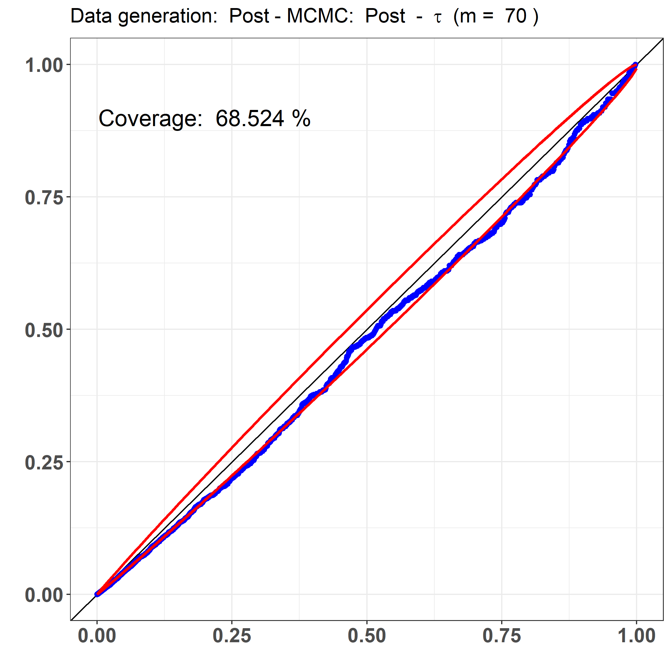
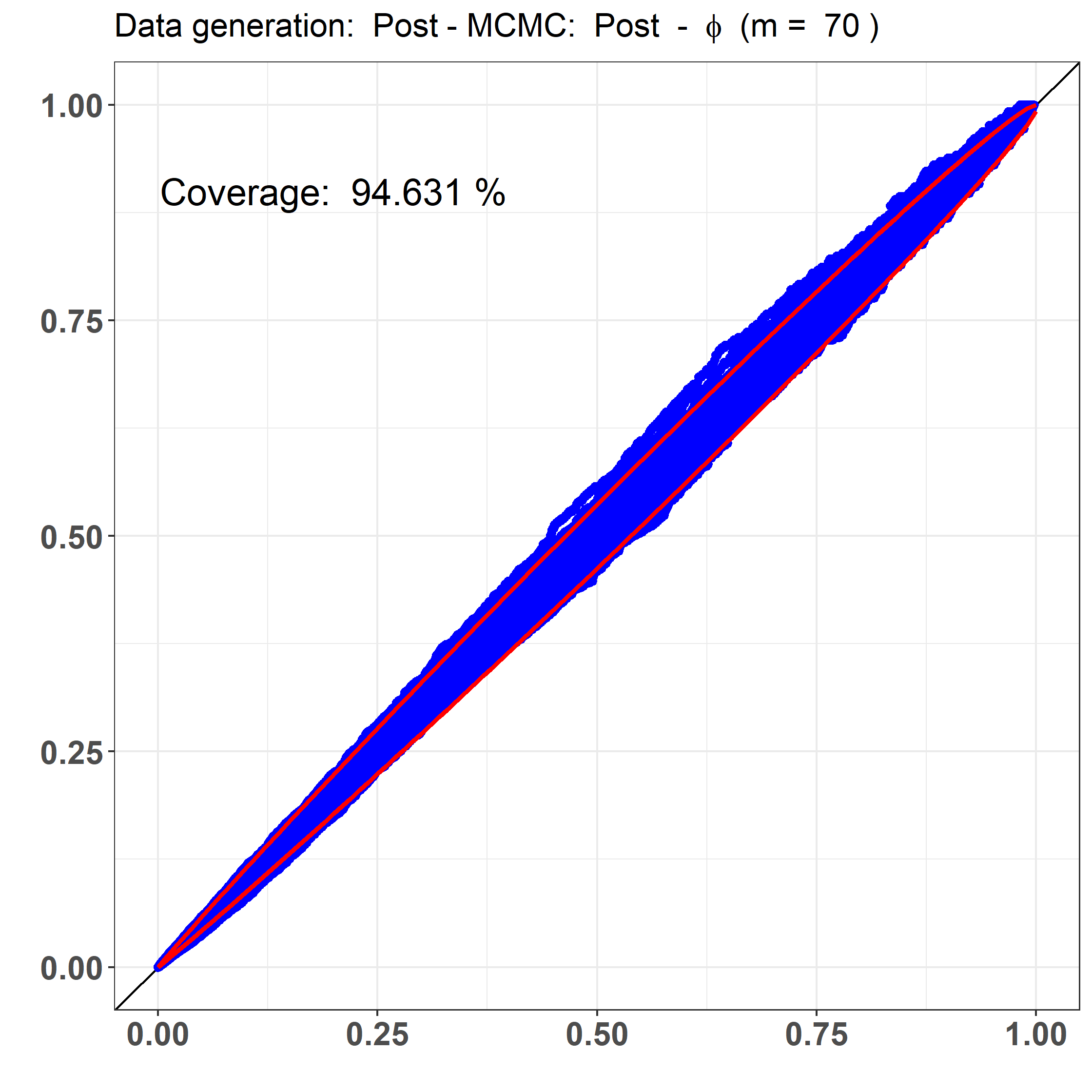
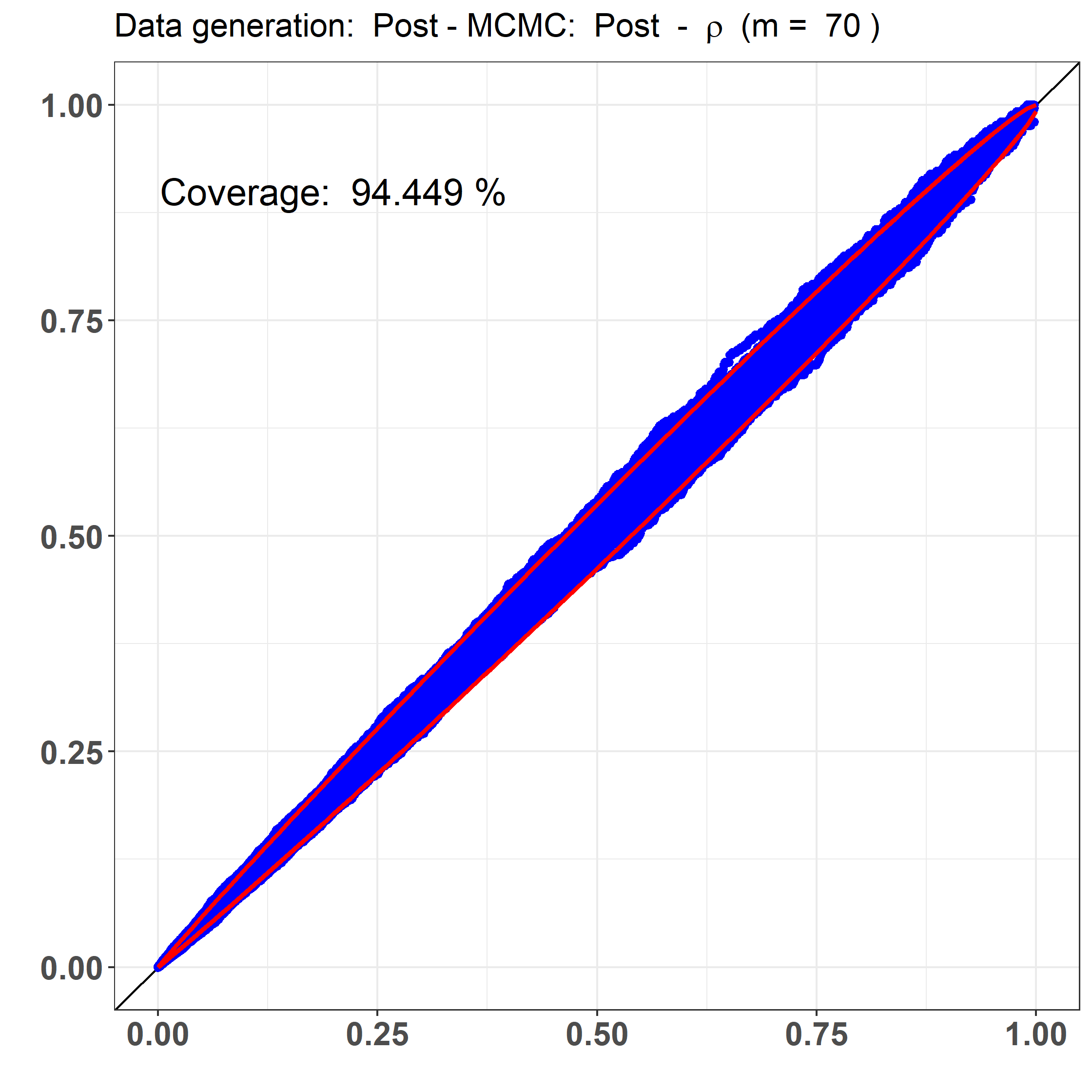
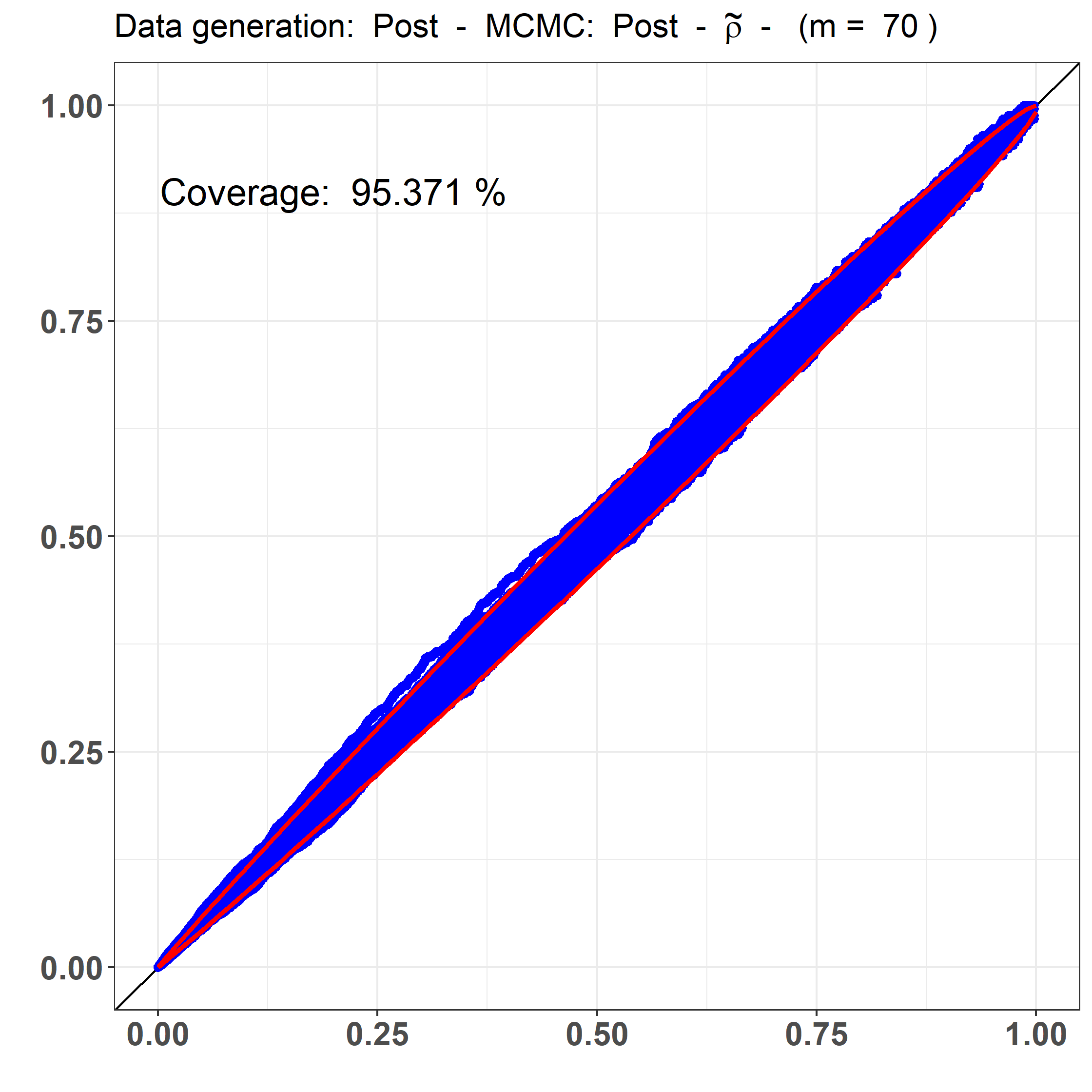
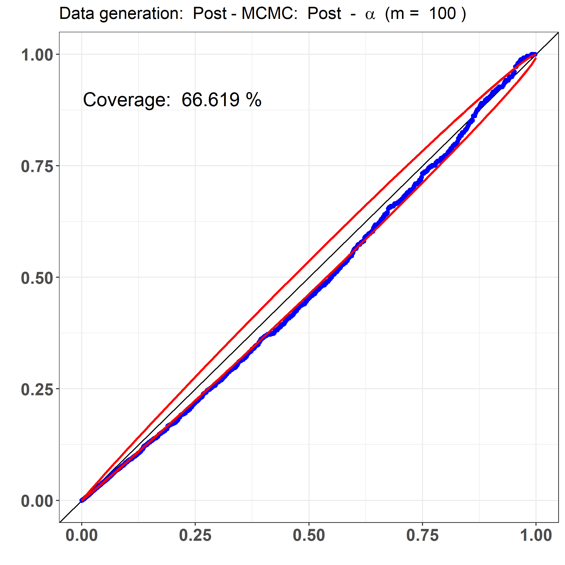
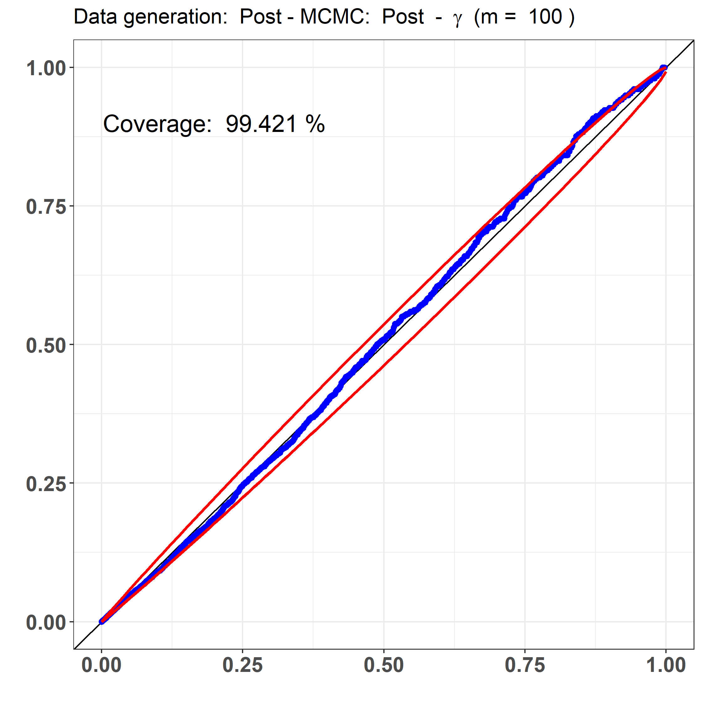
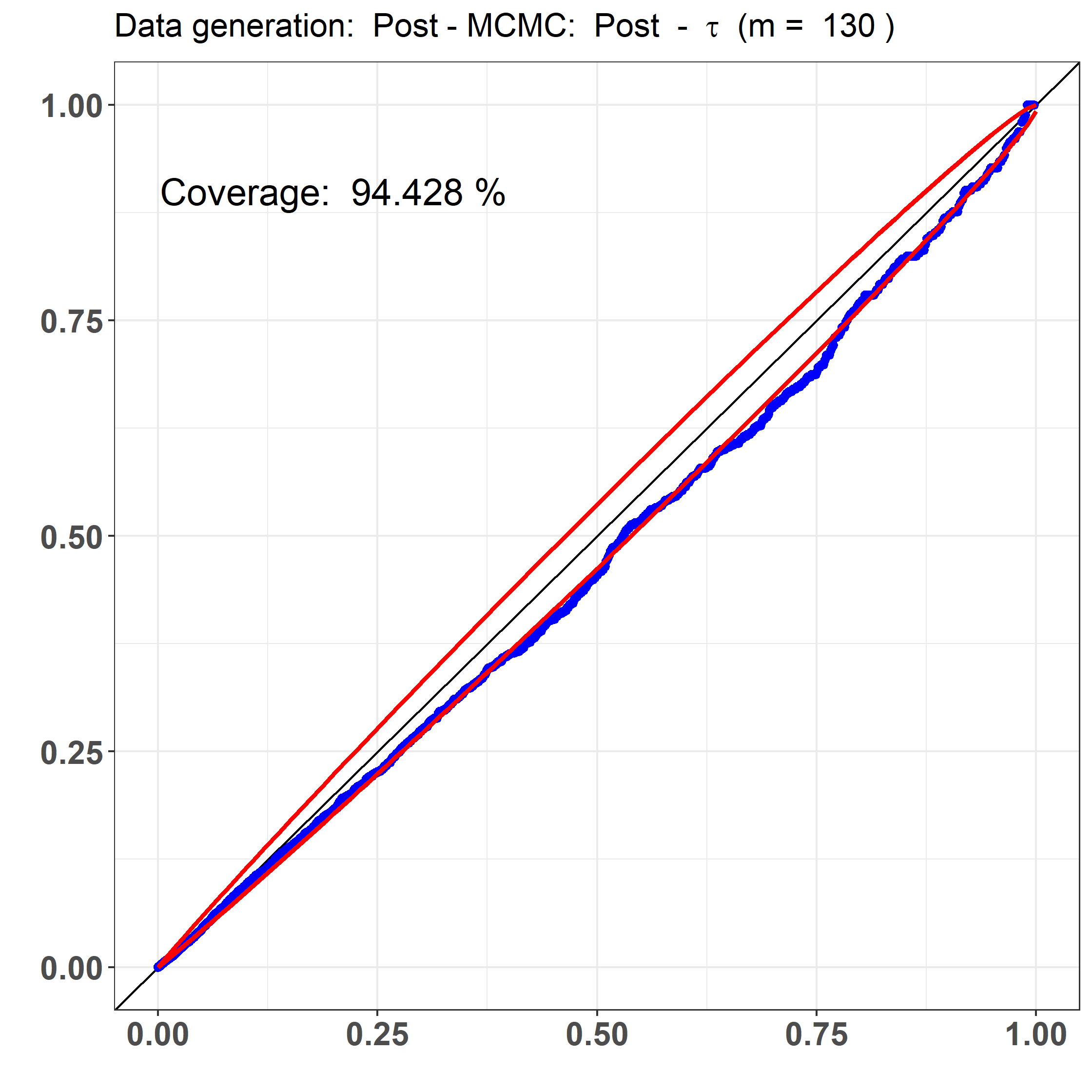
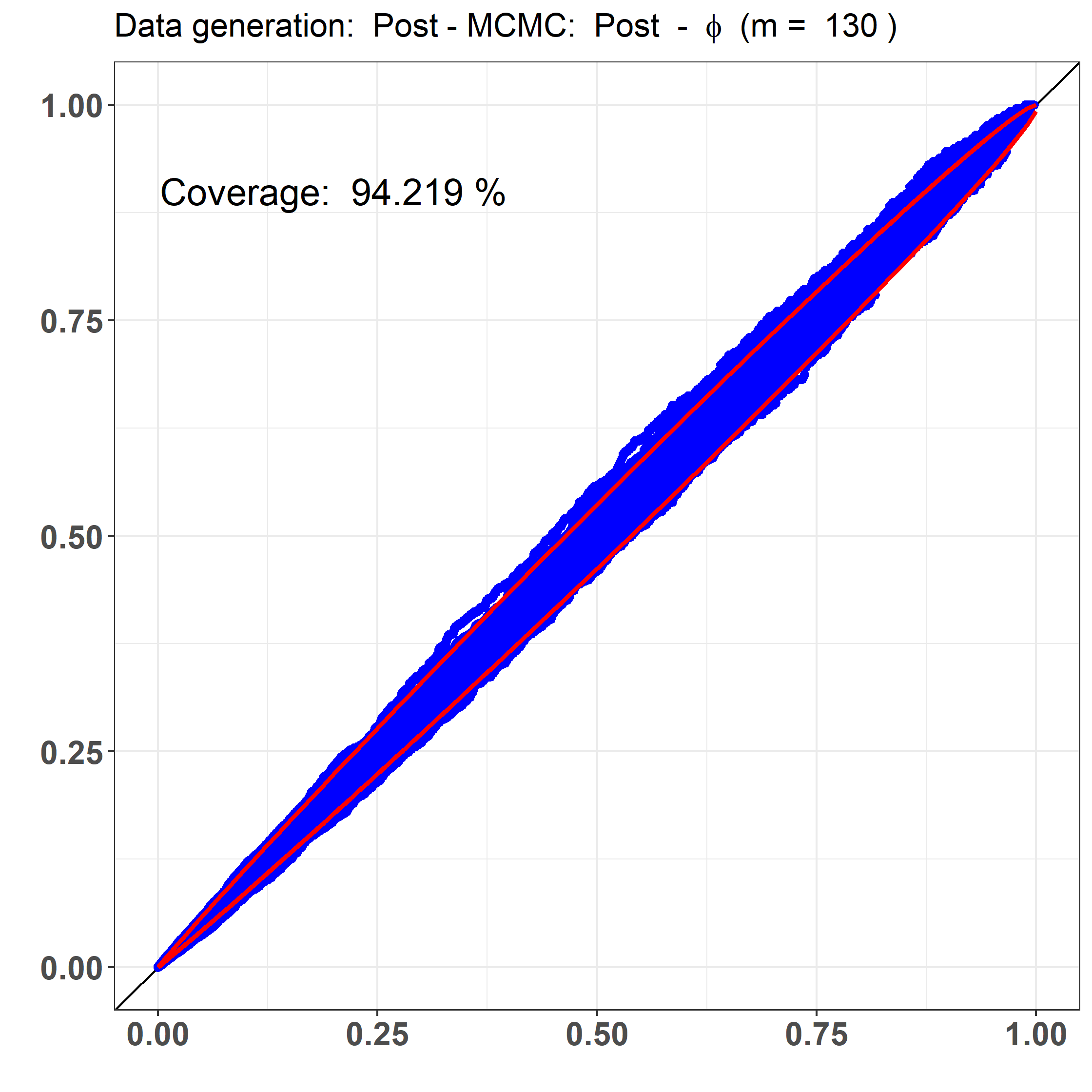
2.3 Calibration plots
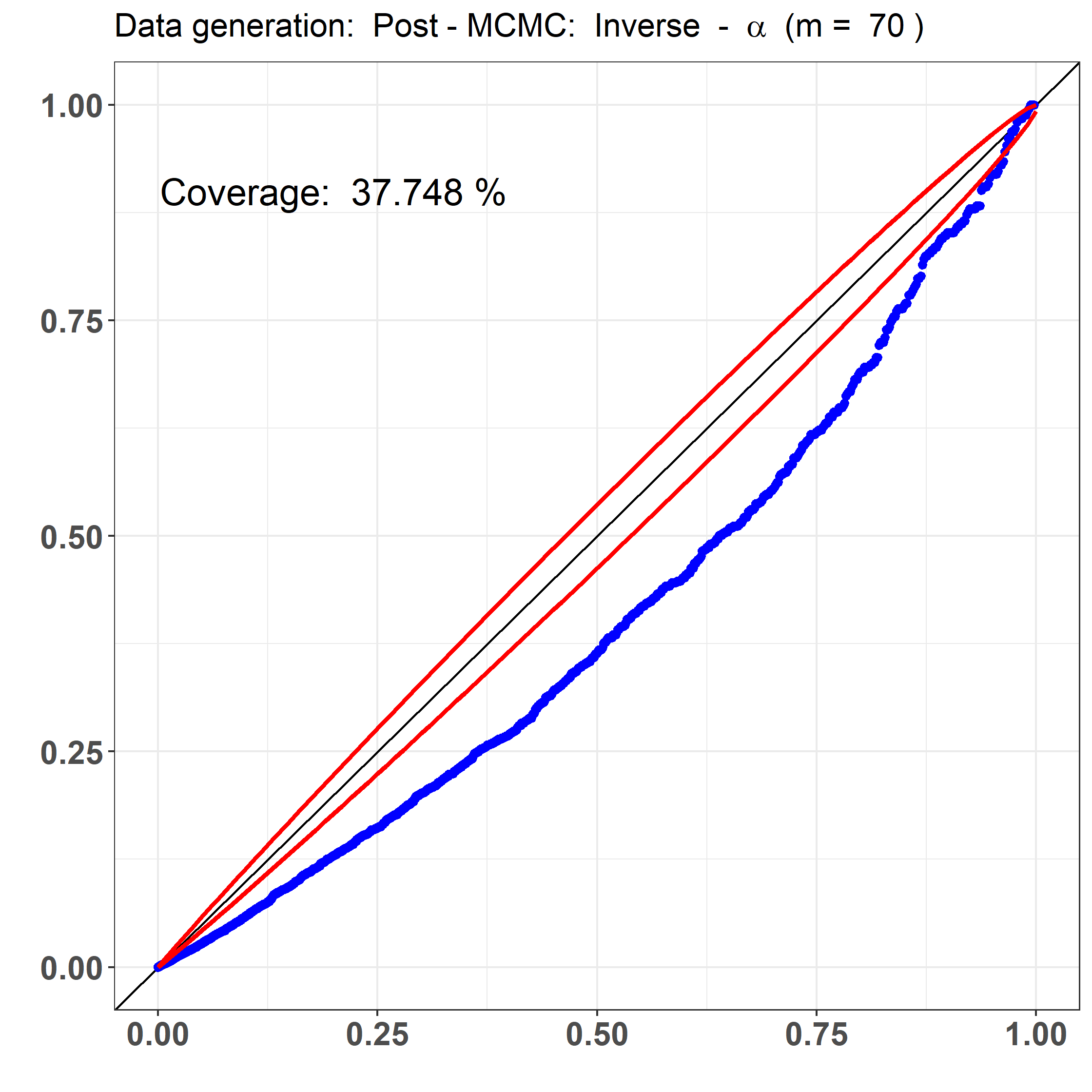
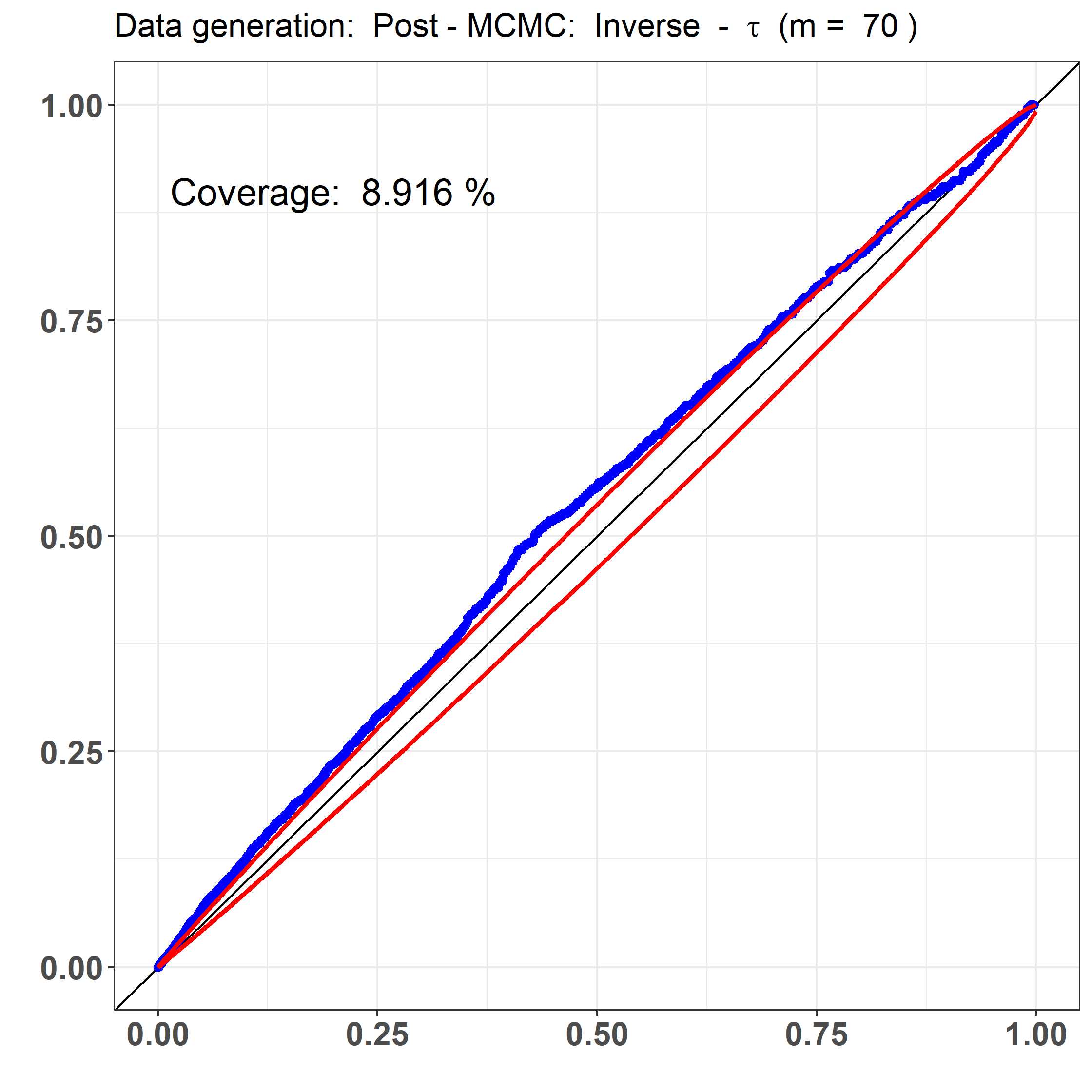
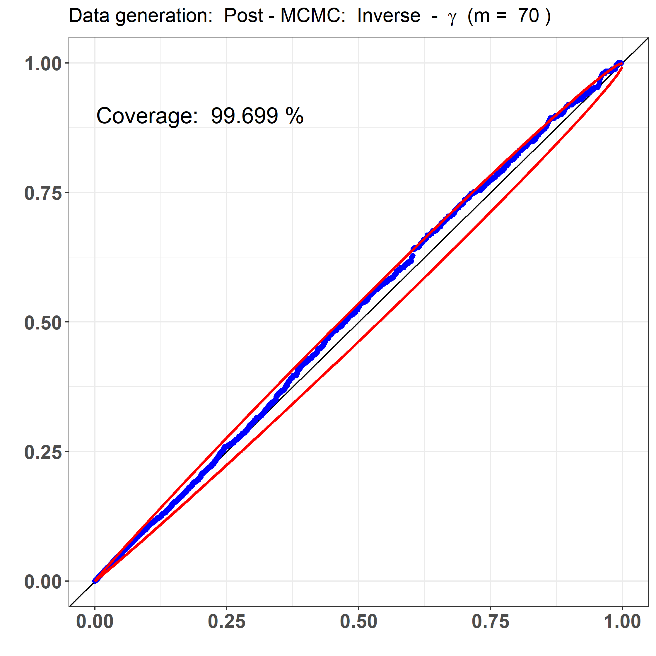
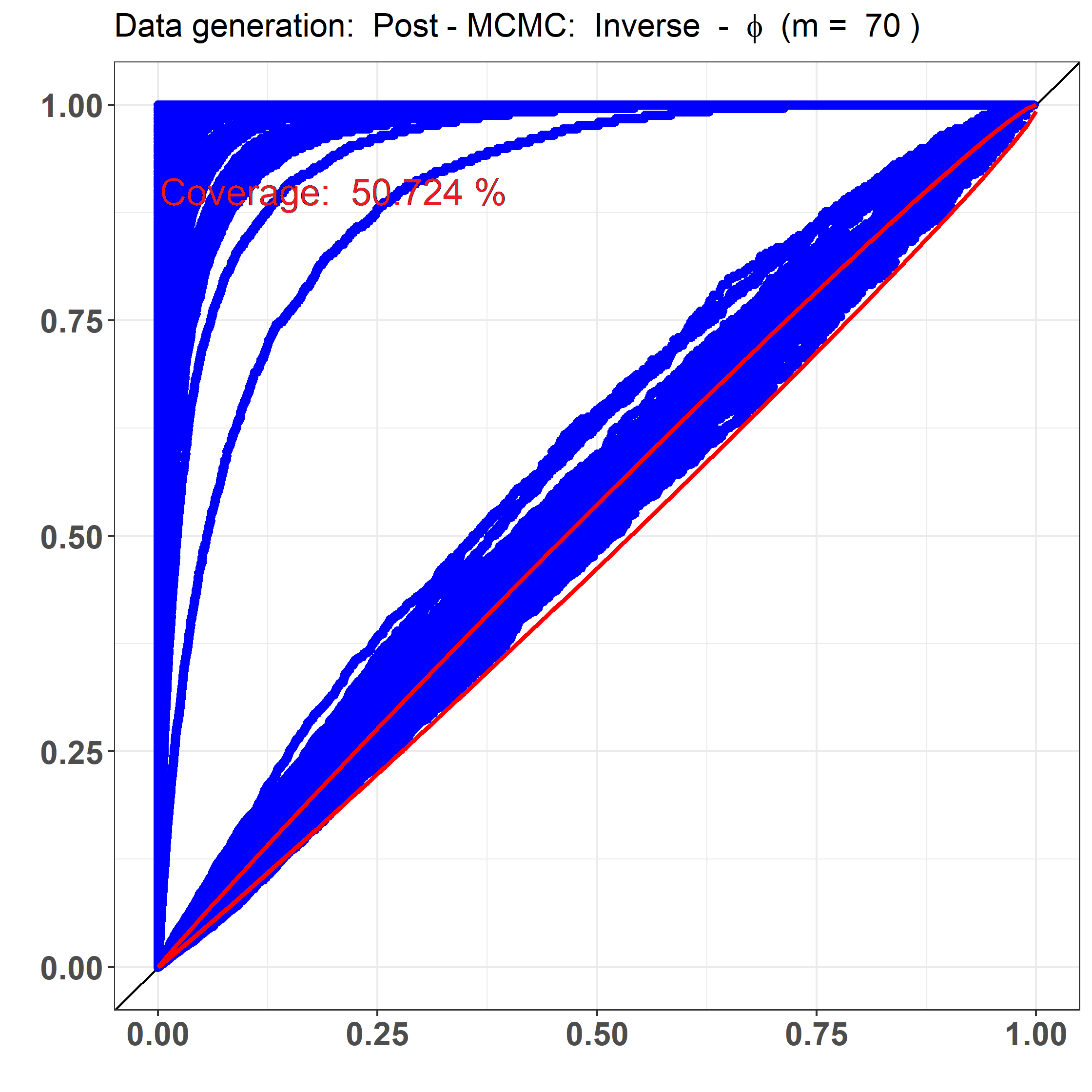
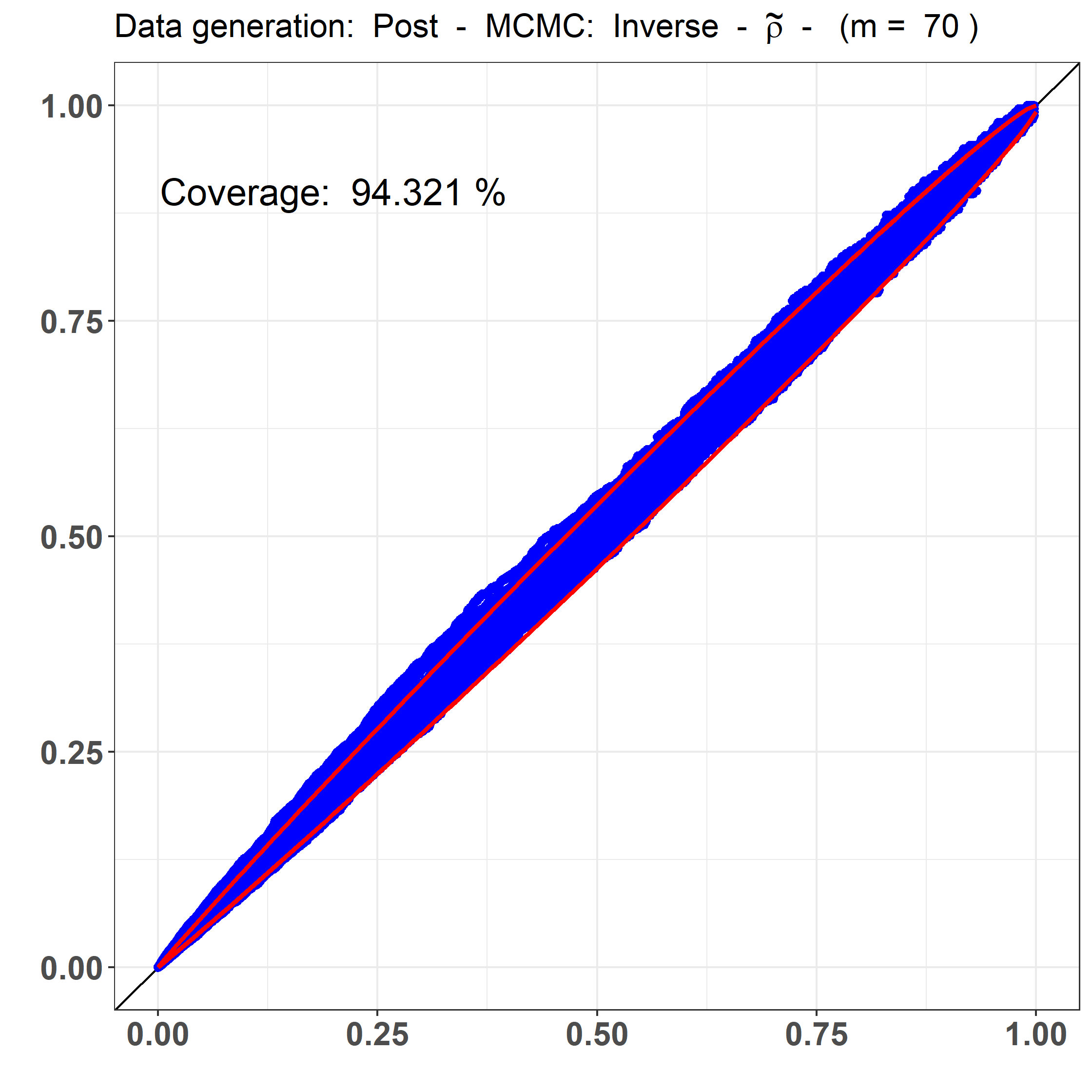
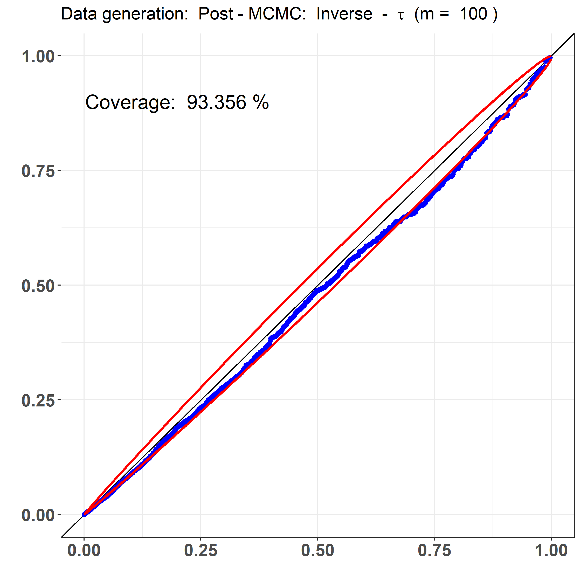
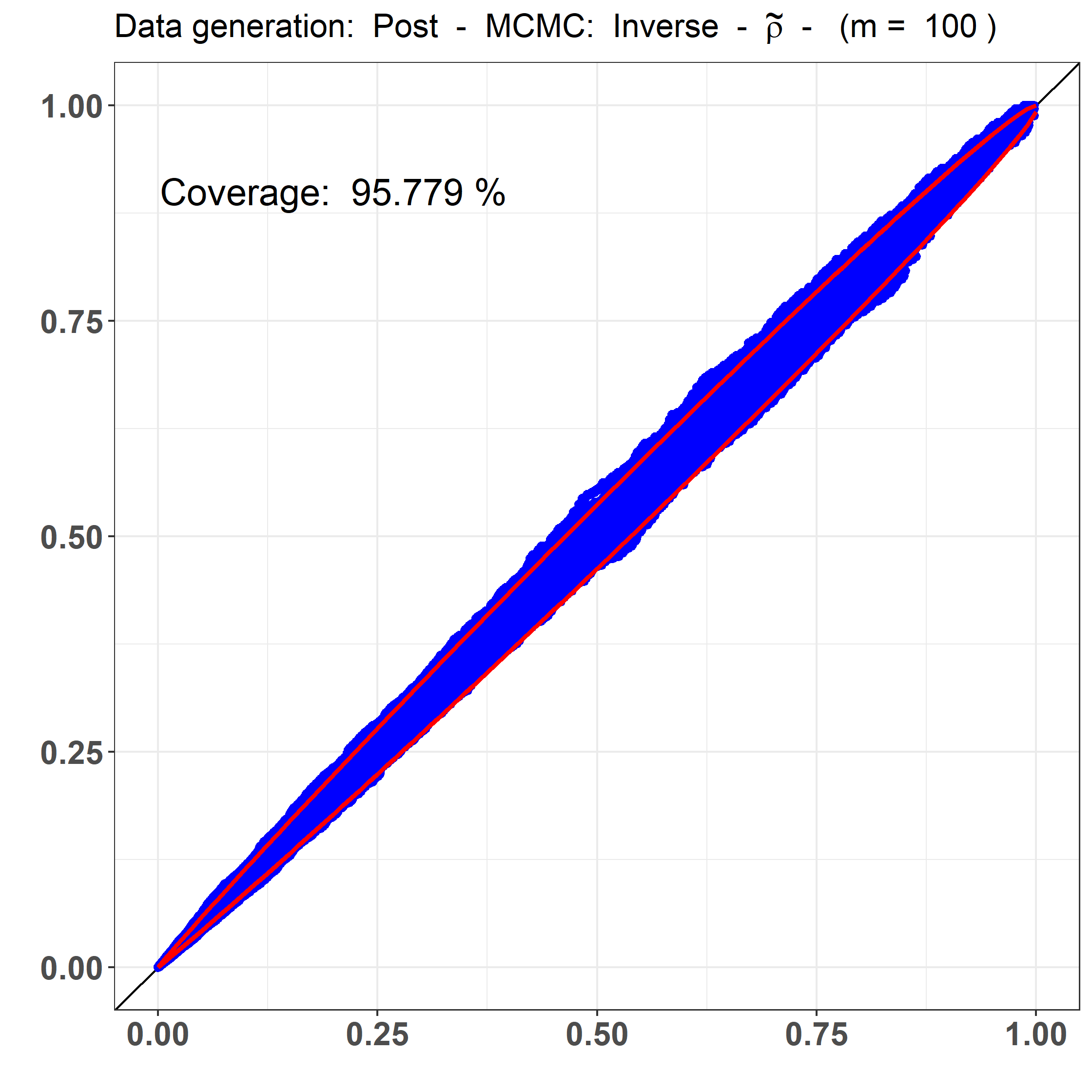
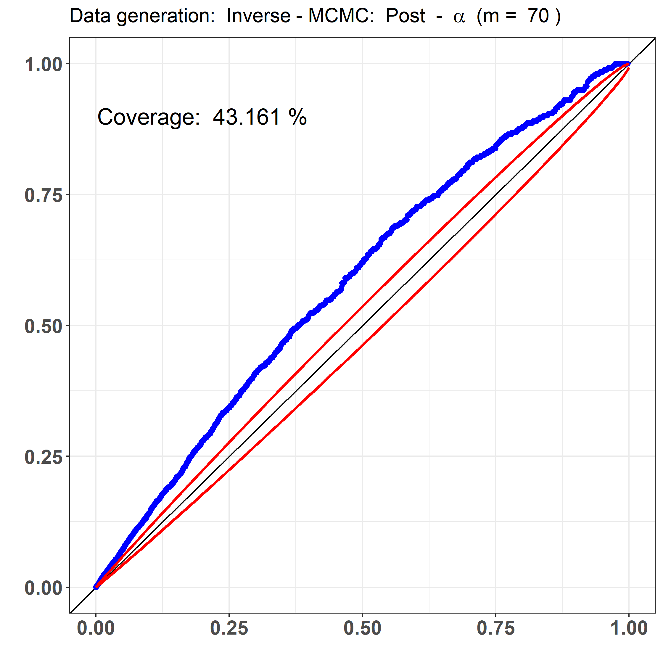
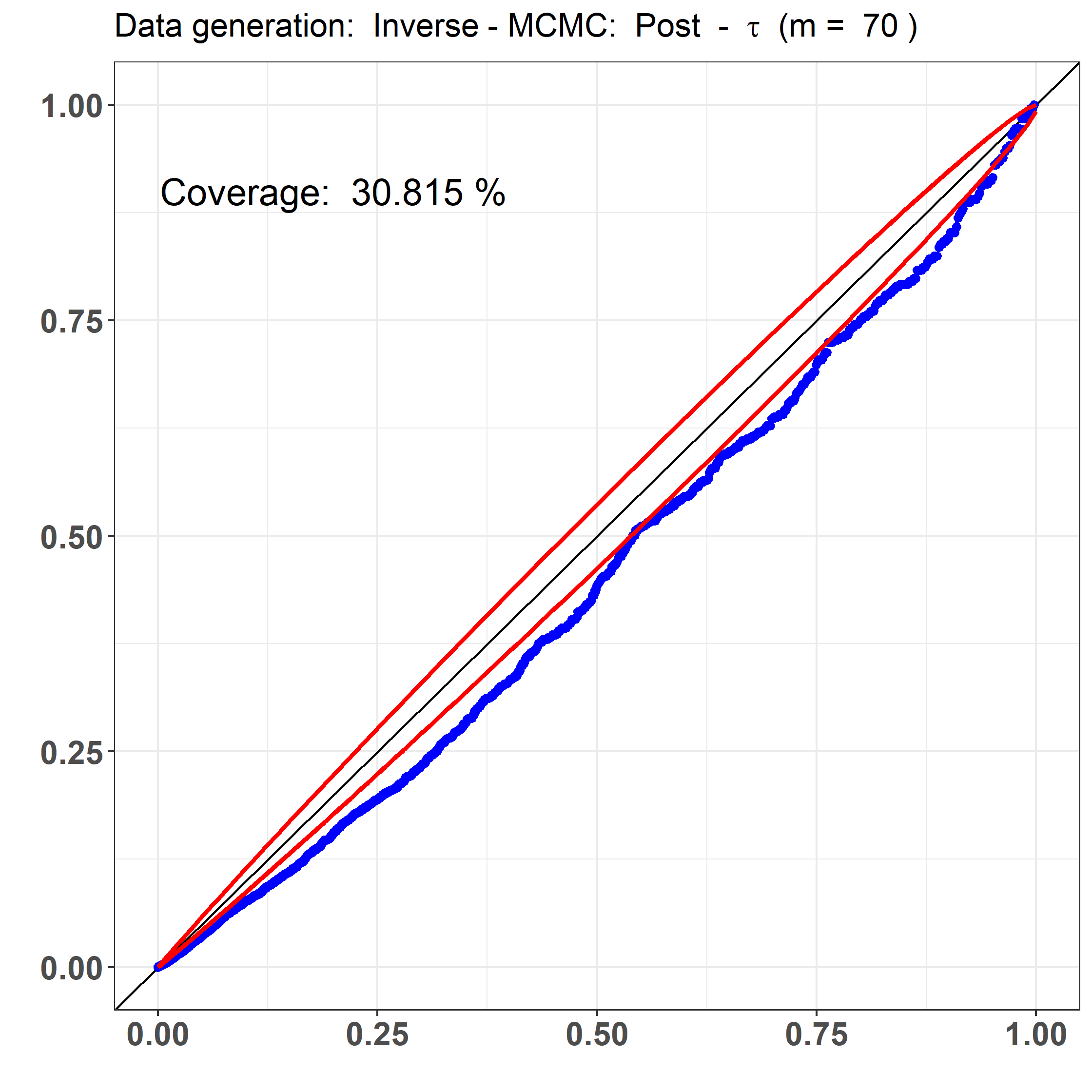
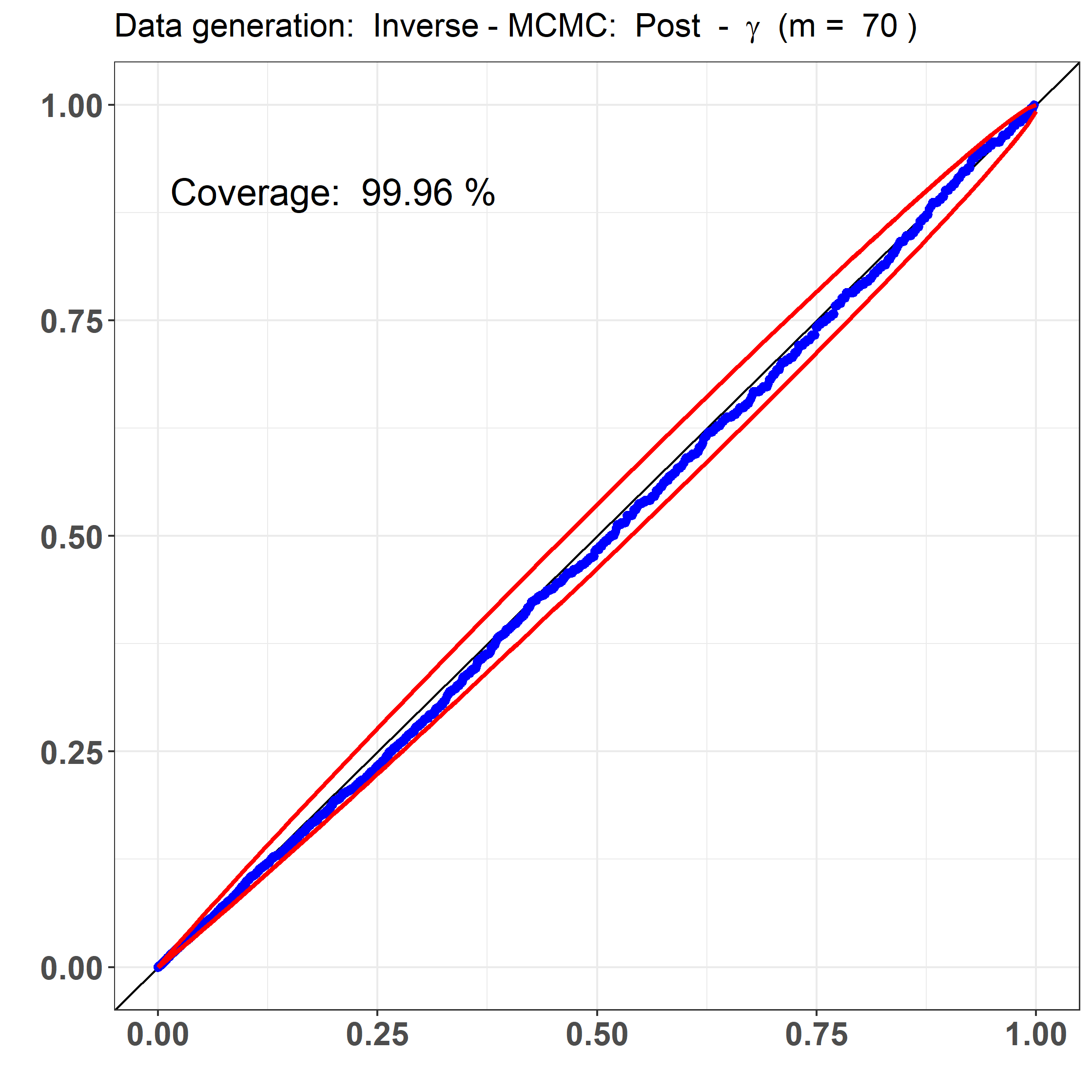
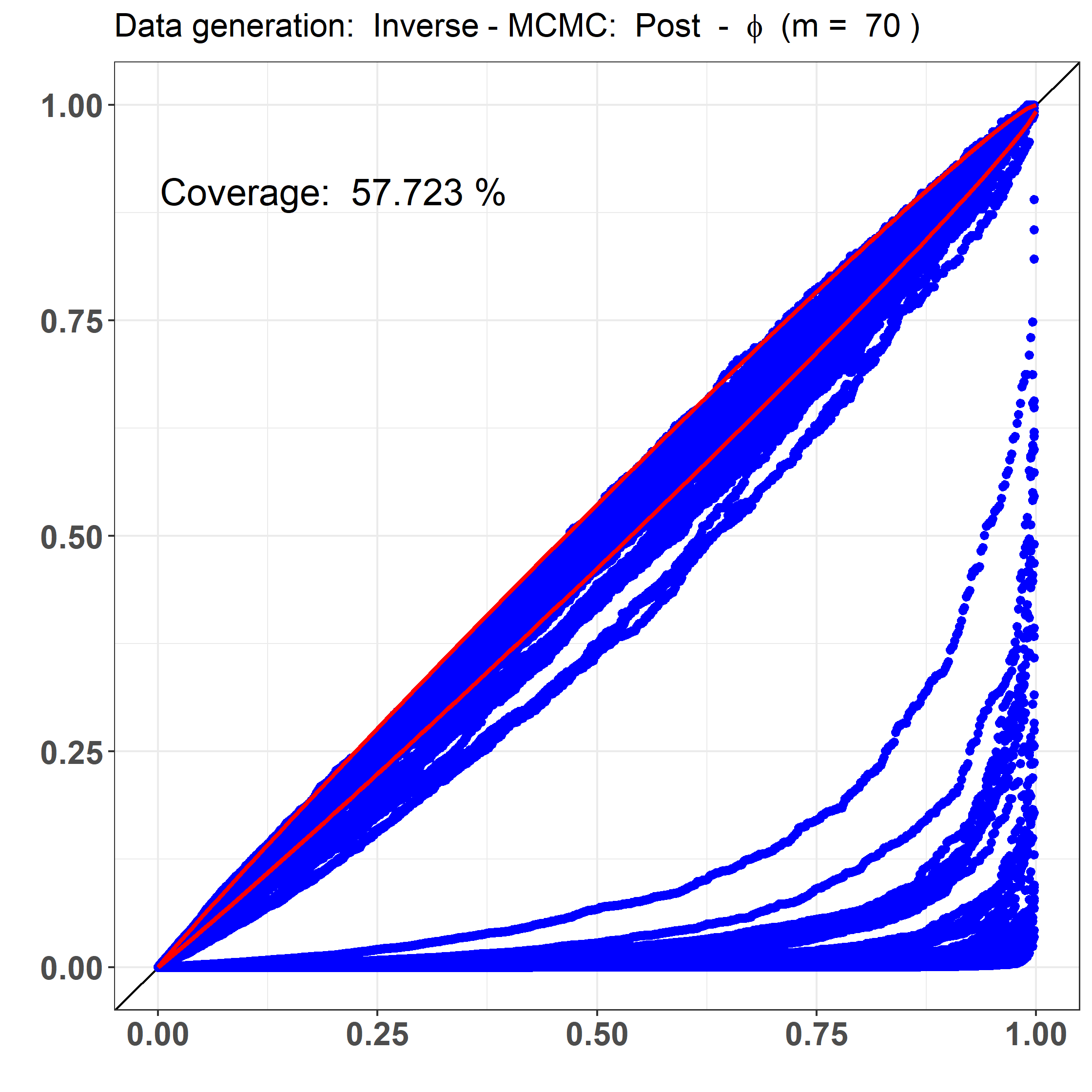
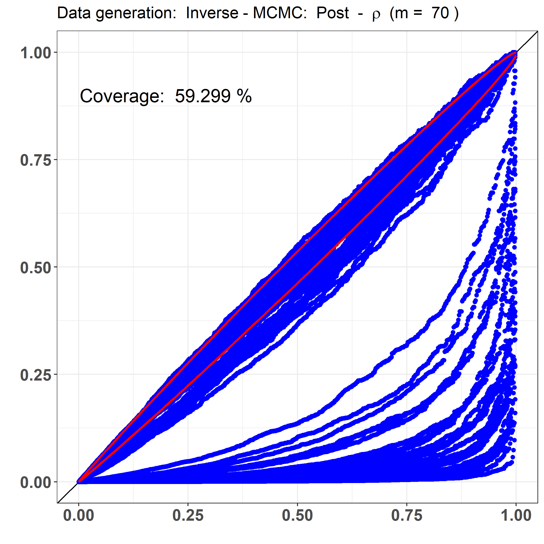
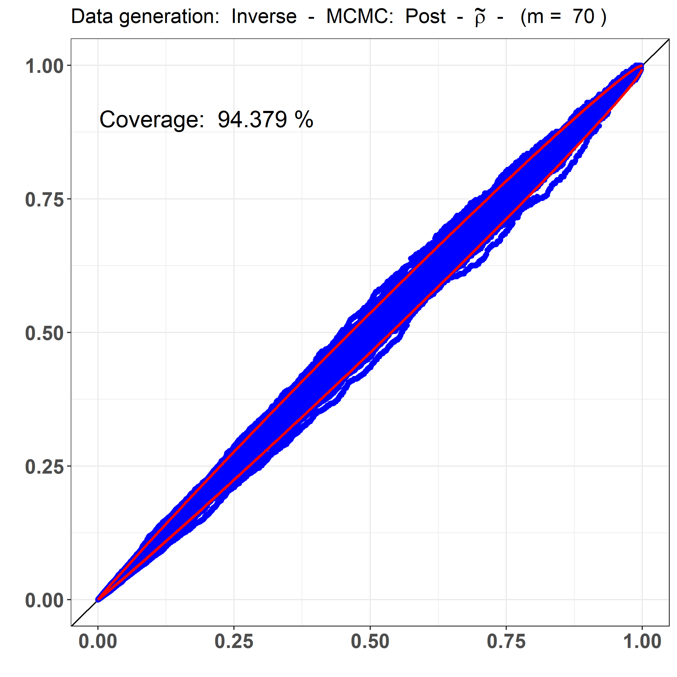
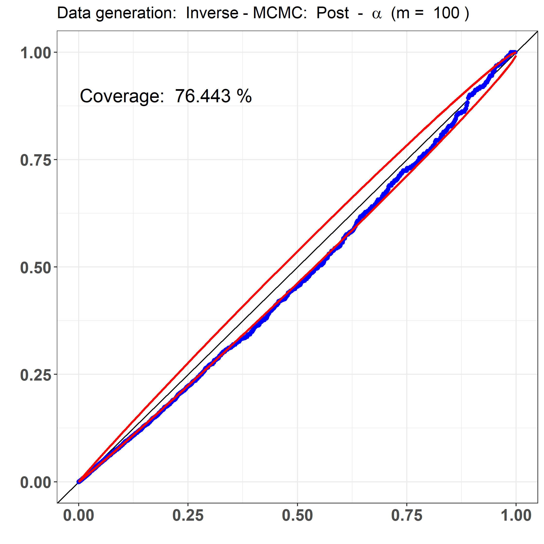
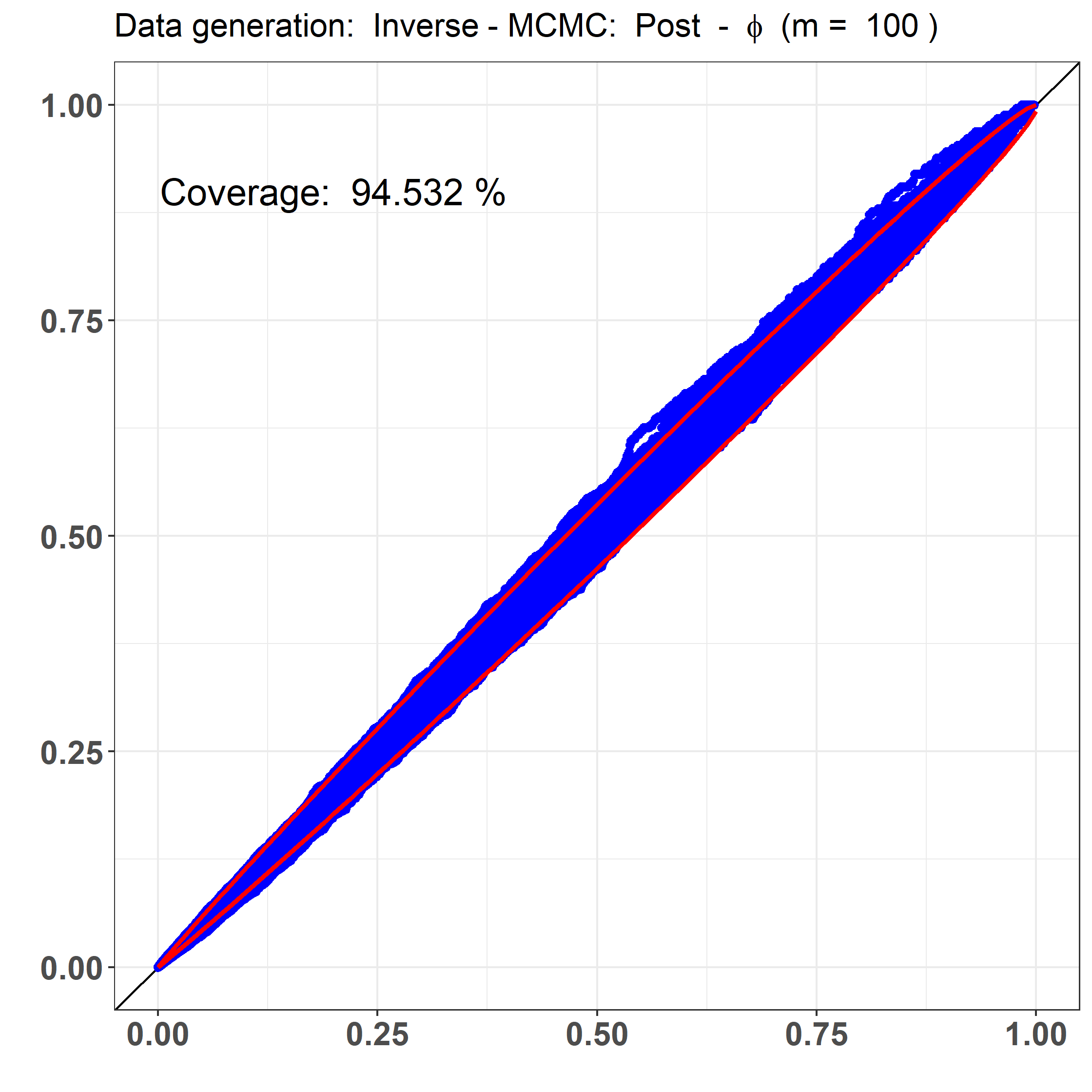
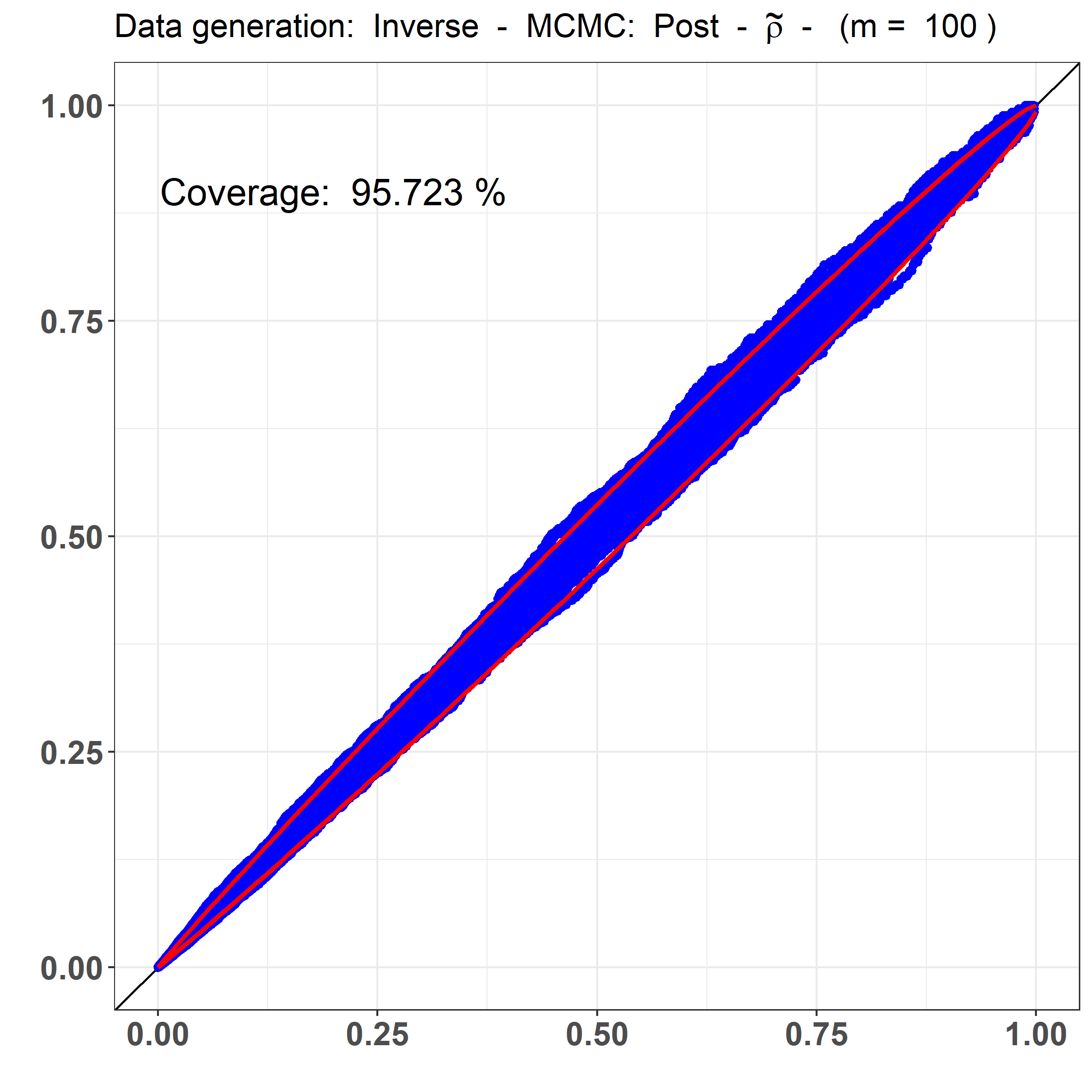
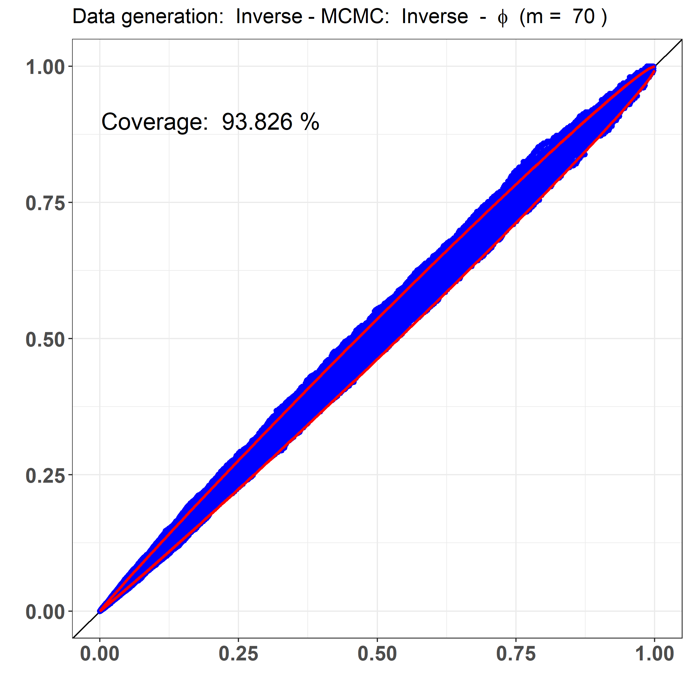
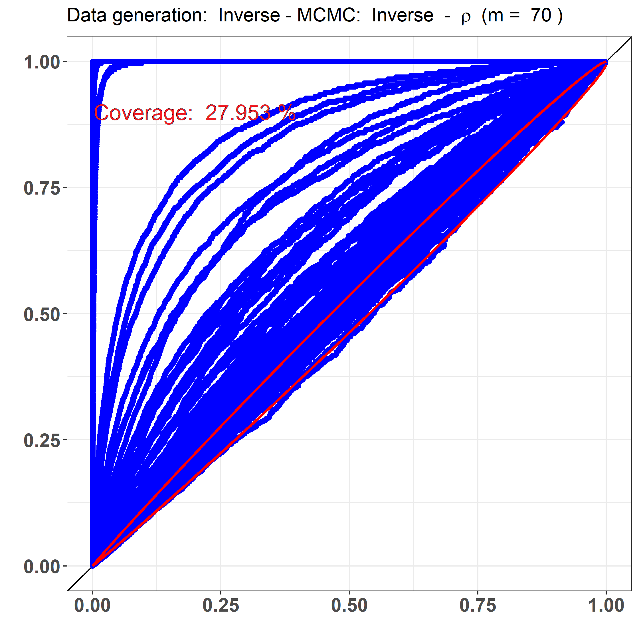
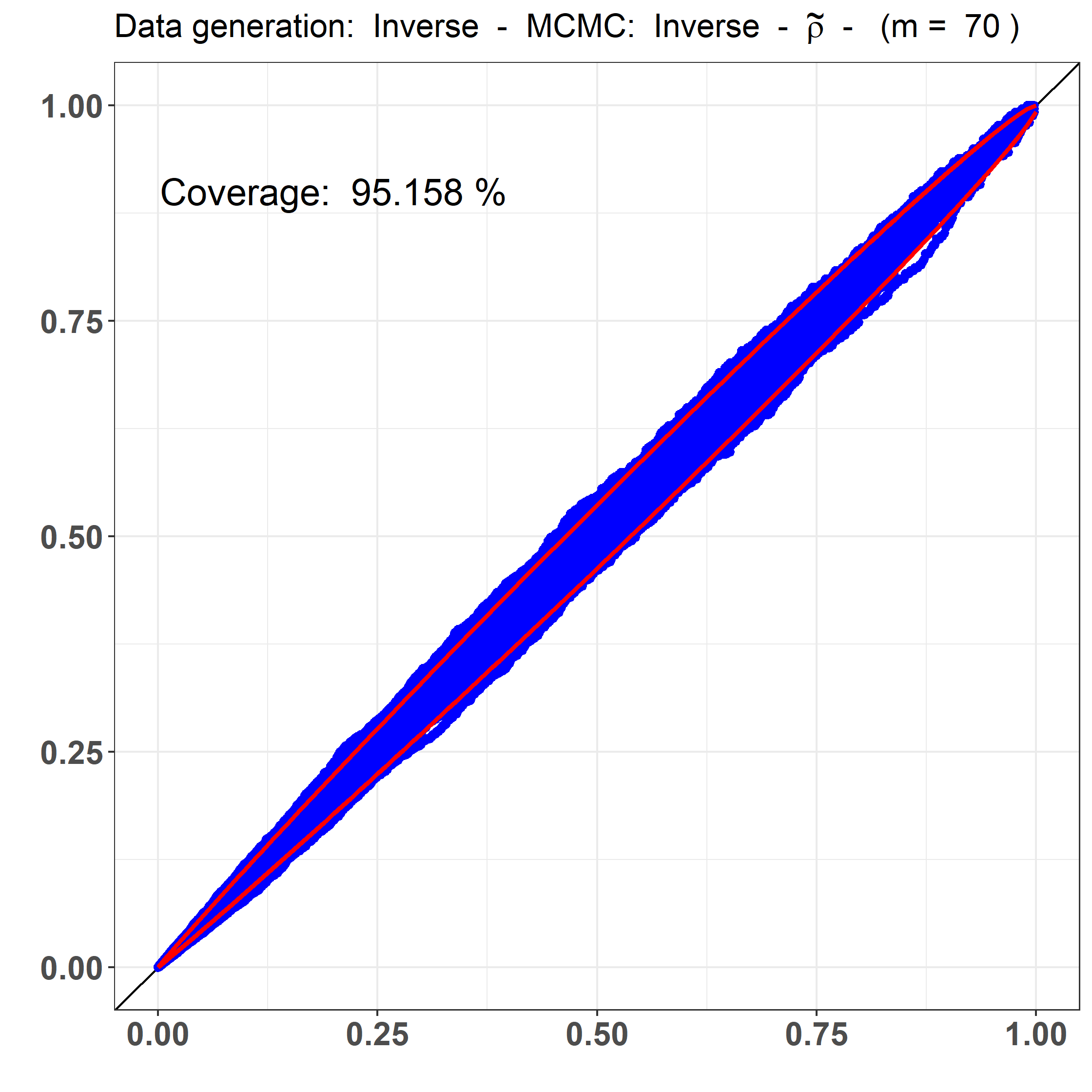
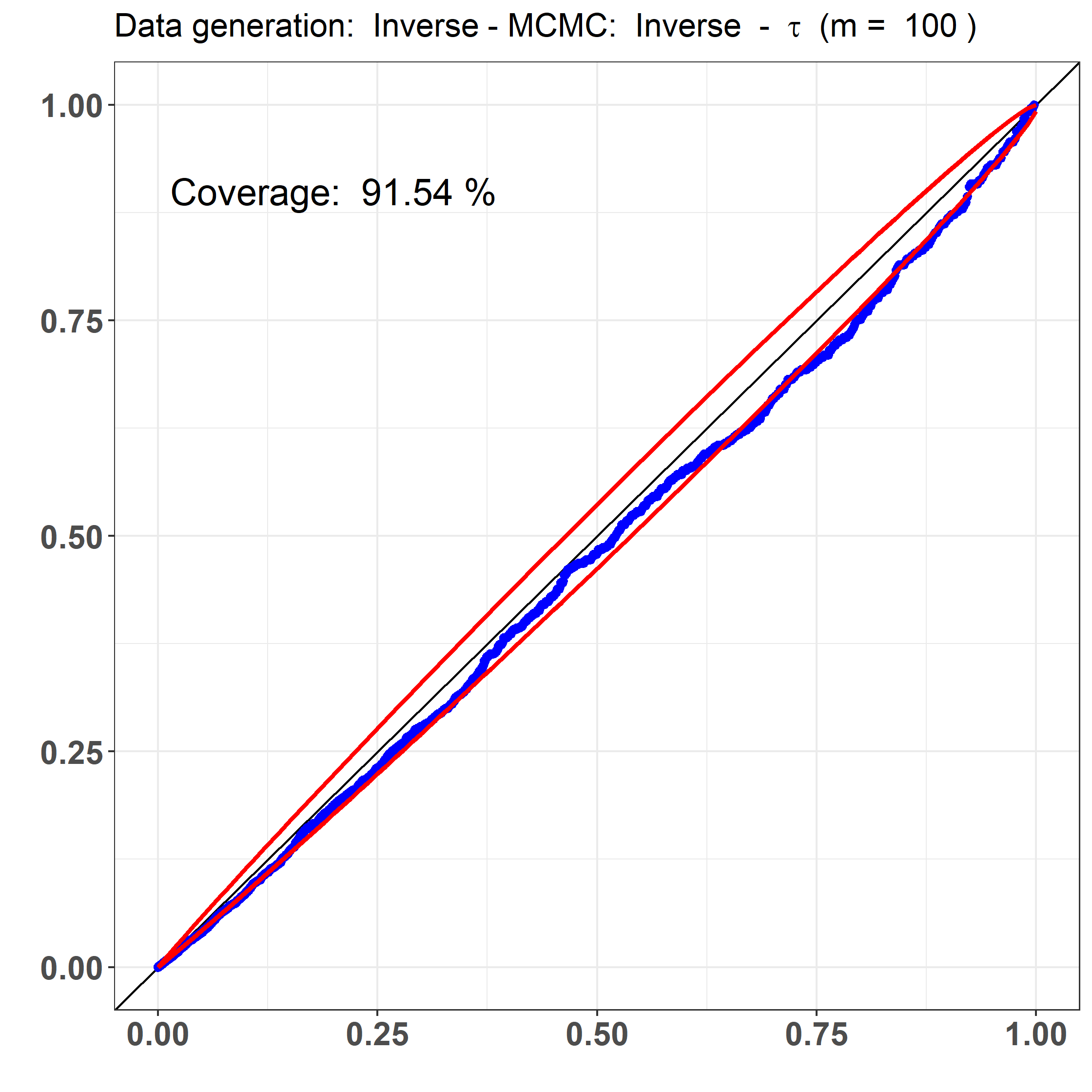
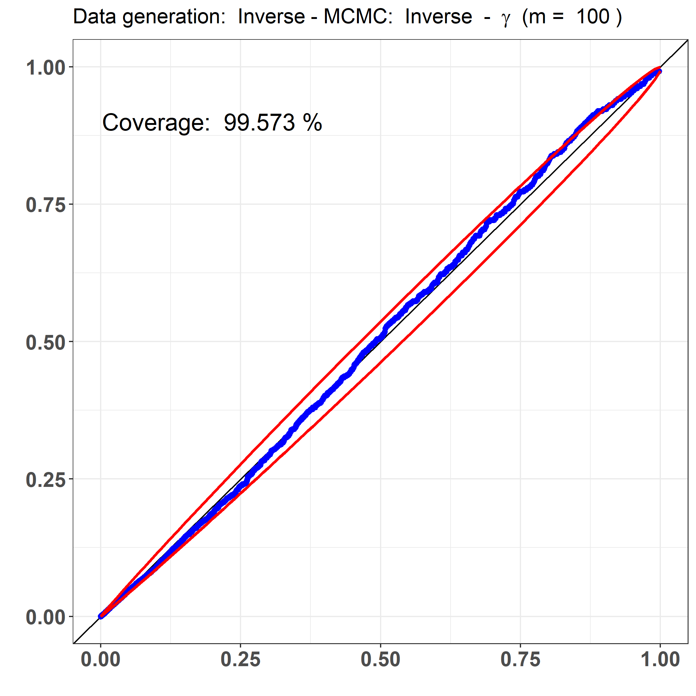
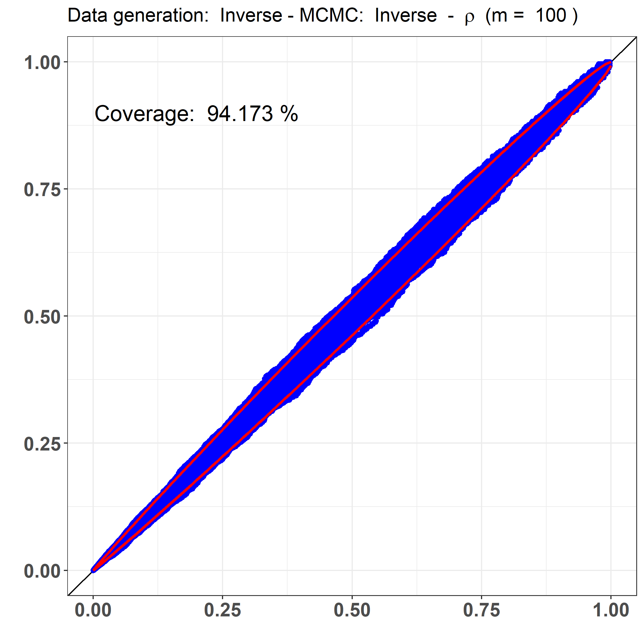
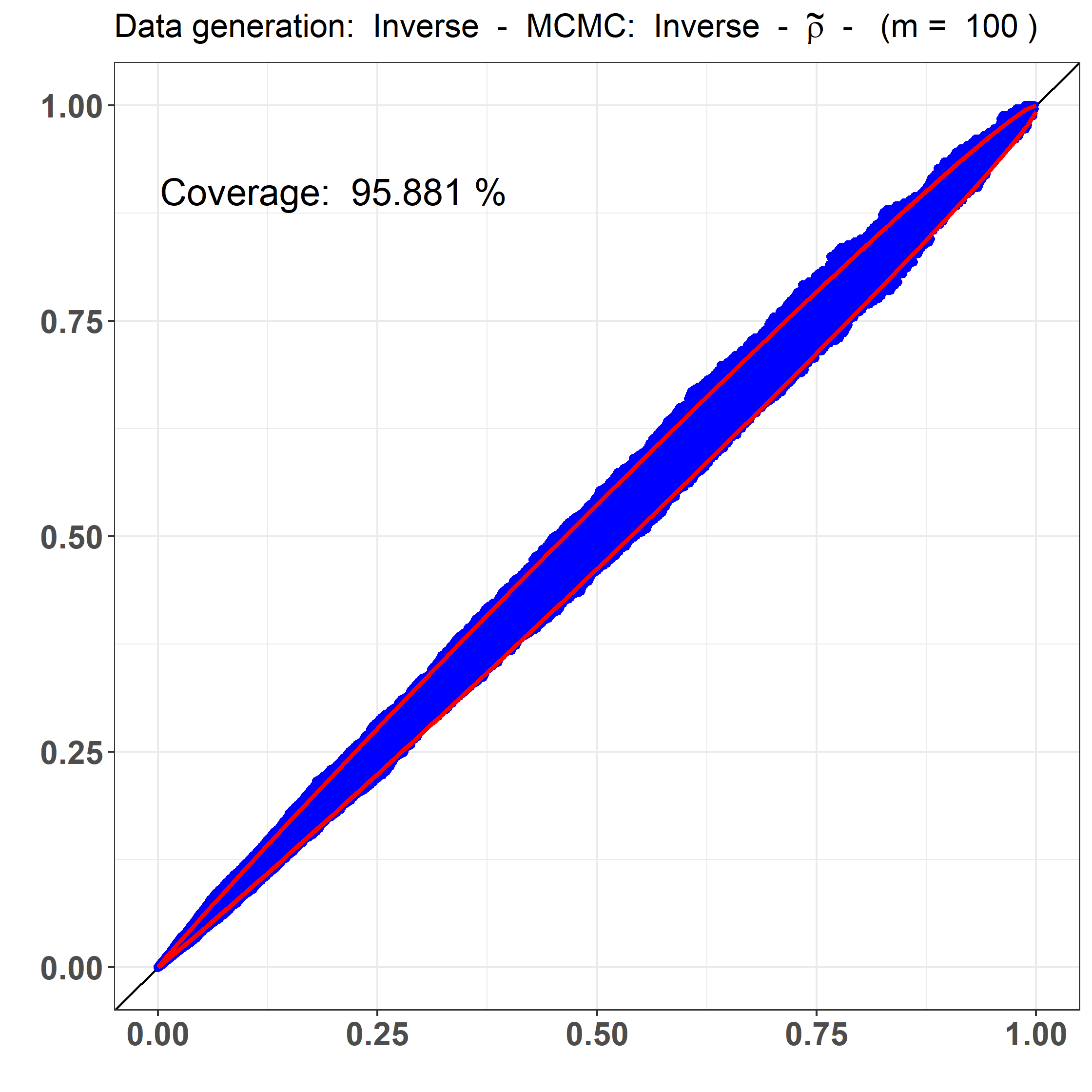
In this Section we report the Q-Q plot of the standardised, i.e. divided by their max , SBC (see Section 5.1) obtained rank statistics against the ordered rank statistics of a discrete uniform distribution with with . Red lines indicate the and quantiles of the ordered rank statistic, which correspond to the 95% expected variation intervals (See also Table 1 for a more compact summary). Quantities on both axes are elevated to the power for improved readability.
Figure 1: Data generation: Post - MCMC: Post -
Figure 2: Data generation: Post - MCMC: Post -
Figure 3: Data generation: Post - MCMC: Post -
Figure 4: Data generation: Post - MCMC: Inverse -
Figure 5: Data generation: Post - MCMC: Inverse -
Figure 6: Data generation: Post - MCMC: Inverse -
Figure 7: Data generation: Inverse - MCMC: Post -
Figure 8: Data generation: Inverse - MCMC: Inverse -
Figure 9: Data generation: Inverse - MCMC: Inverse -
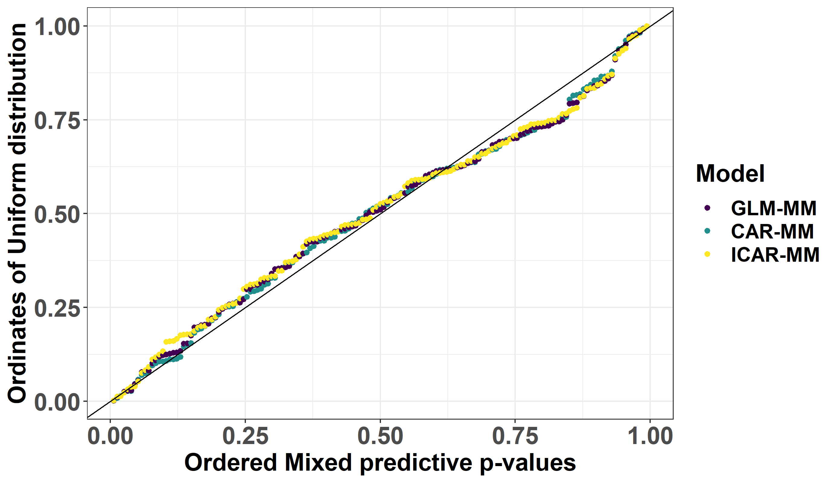
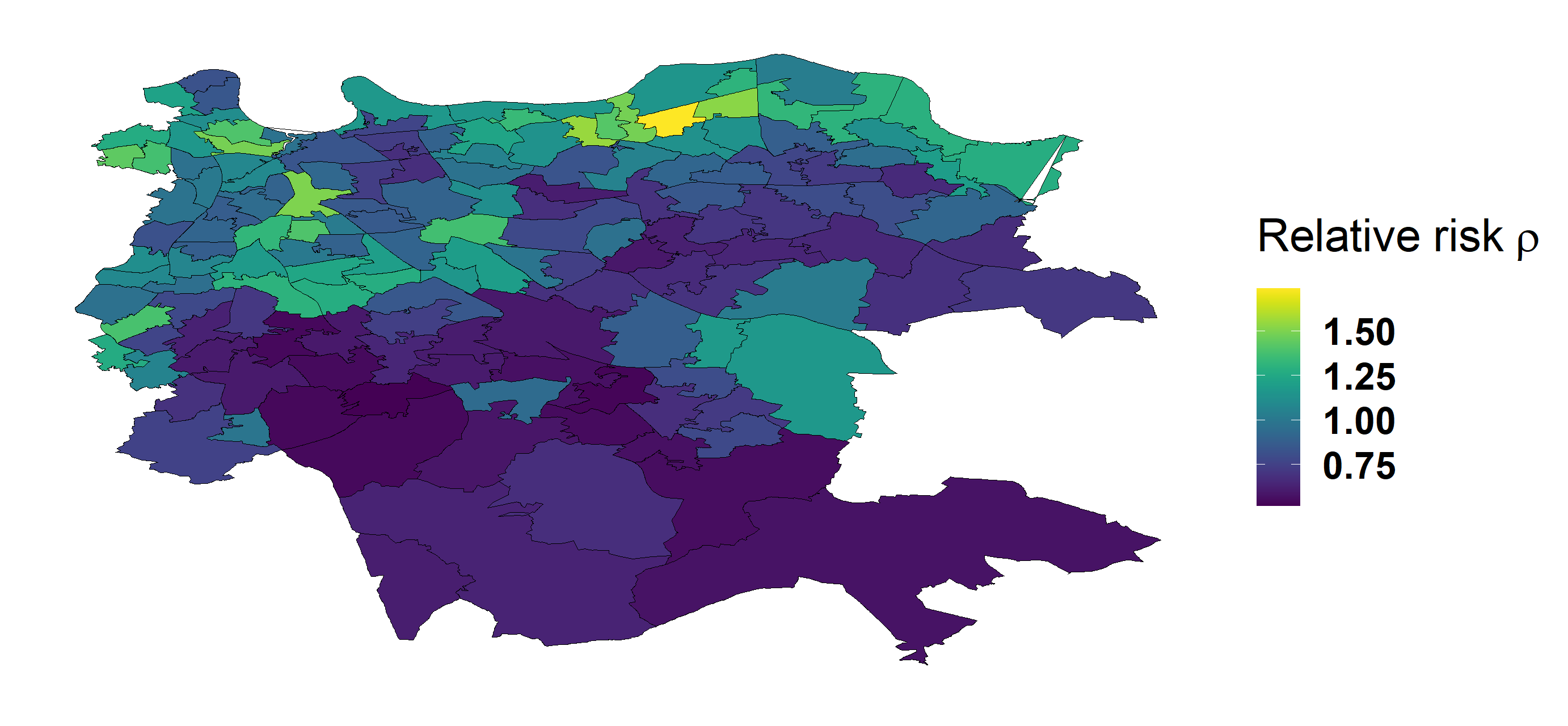
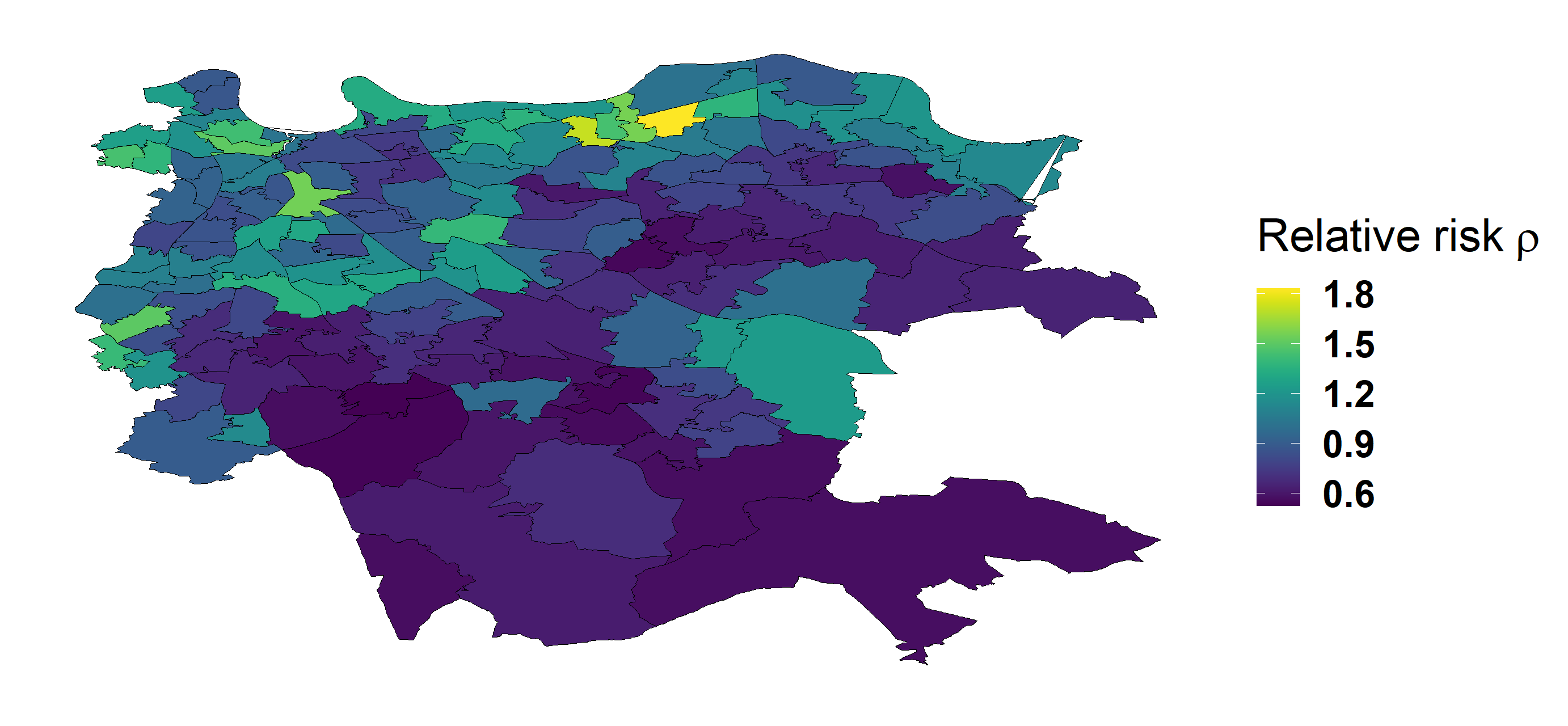
3 Data analysis
Figure 10: Q-Q plots of marginal mixed predictive values versus ordered rank statistic of a uniform distribution for each model run on the SEL datasetFigure 11: Posterior means for each areal relative risk ( in Equation 7.2) for the ICAR-MM modelFigure 12: Posterior means for each areal relative risk ( in Equation 7.2) for the GLM-MM model