The Effects of the Interplay Between Motor and Brownian Forces on the Rheology of Active Gels

Abstract

Active gels perform key mechanical roles inside the cell, such as cell division, motion and force sensing. The unique mechanical properties required to perform such functions arise from the interactions between molecular motors and semi-flexible polymeric filaments. Molecular motors can convert the energy released in the hydrolysis of ATP into forces of up to pico-Newton magnitudes. Moreover, the polymeric filaments that form active gels are flexible enough to respond to Brownian forces, but also stiff enough to support the large tensions induced by the motor-generated forces. Brownian forces are expected to have a significant effect especially at motor activities at which stable non-contractile in vitro active gels are prepared for rheological measurements. Here, a microscopic mean-field theory of active gels originally formulated in the limit of motor-dominated dynamics is extended to include Brownian forces. In the model presented here Brownian forces are included accurately, at real room temperature, even in systems with high motor activity. It is shown that a subtle interplay, or competition, between motor-generated forces and Brownian forces has an important impact in the mass transport and rheological properties of active gels. The model predictions show that at low frequencies the dynamic modulus of active gels is determined mostly by motor protein dynamics. However, Brownian forces significantly increase the breadth of the relaxation spectrum and can affect the shape of the dynamic modulus over a wide frequency range even for ratios of motor to Brownian forces of more than a hundred. Since the ratio between motor and Brownian forces is sensitive to ATP concentration, the results presented here shed some light on how the transient mechanical response of active gels changes with varying ATP concentration.

Universidad de Concepción] Department of Chemical Engineering, Universidad de Concepción, Concepción, Chile IR,NMR,UV

This article may be downloaded for personal use only. Any other use requires prior permission of the author and ACS Publications. This article appeared in A. Córdoba, J. Phys. Chem. B 2018, 122, 15, 4267–4277 and may be found at:
https://doi.org/10.1021/acs.jpcb.8b00238.

1 Introduction

Active gels are networks of semiflexible polymer filaments driven by motor proteins that can convert chemical energy from the hydrolysis of adenosine triphosphate (ATP) to mechanical work and motion. Active gels perform essential functions in living tissue including motions, generation of forces and sensing of external forces. Moreover, active gels play a central role in driving cell division and cell motility ¹, ², ³. For instance, a widely studied active gel is the actin cortex which is a disordered network of F-actin decorated with myosin II motors. Changes in cell shape, as required for migration and division, are mediated by the cell cortex. Myosin II motors drive contractility of the cortical actin network, enabling shape change and cytoplasmic flows underlying important physiological processes such as cell division, migration and tissue morphogenesis ³. Moreover, Actin filaments are enriched beneath the plasma membrane, especially at the pre- and postsynaptic regions in neurons. Among the myosin superfamily proteins, myosin Va, myosin Vb, and myosin VI are primarily involved in transport in the synaptic regions ⁴. Myosin II is also involved in dynamic organization of actin bundles in the postsynaptic spines and is related to synaptic plasticity through control of spine shape ⁴.

The semiflexible filaments that form active gels, such as actin and tubulin, are characterized by having a persistence length (length over which the tangent vectors to the contour of the filament remain correlated) that is larger than the mesh size of the network, but typically smaller than the contour length of the filament. For instance, for filamentous actin (F-actin) the persistence length is around $10\leavevmode\nobreak\ \mu$m, while the mesh size of actin networks is estimated to be approximately $1\leavevmode\nobreak\ \mu$m. ^{5, 6, 7} In active gels, molecular motors assemble into cylindrical aggregates with groups of binding heads at each end that can attach to active sites along the semiflexible filaments that constitute the gel ⁸, ⁹. For example, in actomyosin gels myosin II motors ensemble into cylindrical aggregates of about $1.5\leavevmode\nobreak\ \mu$m in length, each aggregate has around $400$ attachment heads ³. The binding heads of motor proteins can attach to the polymeric filaments that form the gel, in the absence of ATP motor clusters act as passive cross-links between the polymeric filaments that constitute the gel. Moreover, these heads in the motor proteins can also bind to ATP. When ATP molecules are present the heads of the motor proteins to which ATP binds will detach from the site on the filament to where they where attached. Using the chemical energy from the hydrolysis of ATP the detached motor heads will move towards the next attachment site along the filament contour and reattach. The direction in which motors move is determined by the filament structural polarity ¹⁰, ¹¹. In active gels, motor clusters have several binding heads performing this same process. The binding heads on one end of the motor cluster can be walking along a particular filament while the binding heads on the other end of the motor cluster can be attached to a different, neighboring, filament. This second filament will feel a force due to the motion of the motor along the first filament. For instance, in actomyosin gels approximately four out of 400 attachment heads in a myosin motor cluster are attached to an actin filament at any given time. Each motor head can exert $3-4$ pN force, assuming that each motor head contributes force additively, then the whole myosin aggregate can exert roughly $12-16$ pN of force ³ on an actin filament.

Active gels exhibit modulated flowing phases and a macroscopic phase separation at high activity ^{12, 13}. However at low ATP or motor protein concentrations stable active gels have been successfully prepared in vitro to study their mechanical and rheological properties ^{14, 15, 16, 17}. The rheological properties of active gels have also been studied in vivo. For instance the motility of Amoeba proteus was examined using the technique of passive particle tracking microrheology ¹⁸. Endogenous particles in the amoebae cytoplasm were tracked, which displayed subdiffusive motion at short timescales, corresponding to Brownian motion in a viscoelastic medium, and superdiffusive motion at long timescales due to the convection of the cytoplasm. The subdiffusive motion of tracer particles was characterized by a rheological scaling exponent of $3/4$ in the cortex, indicative of the semiflexible dynamics of the actin fiber. The mechanical properties of embryos of Drosophila in early stages of development have also been recently studied using microrheology ¹⁹.

These rheological experiments in active polymeric networks have revealed fundamental differences from their passive counterparts. For instance, it has been observed that the fluctuation-dissipation theorem (FDT) is violated in active gels ¹⁵, ¹⁴, ¹⁶. This violation shows up as a frequency-dependent discrepancy between the material response function obtained from driven and passive microrheology experiments. The discrepancy is largest at low frequencies, around 1 Hz, but it disappears at larger frequencies, around 100 Hz. In driven microrheology an external force is applied to the probe bead and the material response function is calculated from the bead position signal. On the other hand, in passive microrheology experiments, no external force is applied, and the material response function is calculated from the bead position autocorrelation function using the FDT ¹⁶.

Recently a model of active gels that can predict this violation of the FDT in active gels was proposed ^{20, 21}. In the active single-chain model, molecular motors are accounted for by using a mean-field approach and the stochastic state variables evolve according to a proposed differential Chapman-Kolmogorov equation. Initially the model was introduced with a level of description that had the minimum set of variables necessary to describe some of the most characteristic mechanical and rheological properties of active gels ²⁰. For instance, only the simplified case of dumbbells was considered, meaning that only two motor attachment sites per filament were allowed. The filaments were modeled as Fraenkel springs, and the motor force distribution was made a Dirac delta function centered around a mean motor stall force. With those assumptions it was possible to obtain closed-form analytical expressions for several observables of the model, such as relaxation modulus and fraction of buckled filaments. Later, some of the assumptions made in the original model were relaxed ²¹. More specifically, bead-spring chains with multiple attachment sites, finite-extensibility of the filament segments and experimentally-observed motor force distributions were considered. In that form the model can not longer be solved analytically and numerical simulations are employed.

An important simplification in previous versions of the active single-chain model was that Brownian forces were neglected. This simplification was assumed to be appropriate when motor-generated forces are much larger than Brownian forces. However, the model without Brownian forces rendered only a qualitative description at ATP concentrations at which stable non-contractile in vitro active gels are prepared for rheological measurements. The main reason for excluding Brownian forces from the original single-chain active model was to draw a clear distinction between the proposed model and a widespread approach for the mesoscopic modeling of active systems which utilizes a so-called effective temperature. In that approach the motor generated forces are modeled as Brownian forces, but an effective temperature is introduced, which is higher than the real temperature and is meant to account for the larger magnitude of the non-equilibrium fluctuations ^{22, 23, 24, 25}. In this work Brownian forces are included in the active single-chain model, but is important to emphasize that no effective temperature is introduced and the dynamics of the motor-generated forces are treated in the same way that was done in previous versions of the model. This allows for the Brownian forces to be modeled accurately, at real room temperature, even in systems with high motor activity.

The purpose of this work is to provide molecular-level insight into how the interplay, or competition, between Brownian forces and motor-generated forces influence the mass transport and rheological properties of active gels. For this purpose the single-chain model for active gels is extended to include Brownian forces. The paper is organized as follows. It begins with a brief description of the active single-chain model with Brownian forces, discussing the main assumptions, and parameters. An outline of the numerical procedure used to solve the model is also provided there. This is followed by a subsection where the predictions of the active single-chain model for the mass transport mechanisms of filaments in active gels are presented and discussed. It is shown that the model predictions have good qualitative agreement with observations in microtubule and kinesin solutions. This is followed by a subsection where the dependence of the dynamic modulus of active gels on the ratio between motor and Brownian forces is discussed. Also the creep compliance predicted by the active single-chain model with Brownian forces is compared to published microrheology data for actomyosin gels.

2 Results and discussion

2.1 The active single-chain model

The active single-chain model follows a probe filament and approximate its surroundings by an effective medium of motor clusters that attach and detach from specific sites along the probe filament. The motors are assumed to form pair-wise interactions between filaments. When a motor is attached to the probe filament it is stepping forward on another filament in the mean-field and therefore pulls/pushes on the probe filament. To model these interactions a mean-field approach is employed, in which filaments have prescribed probabilities to undergo a transition from one attachment/detachment state into another depending on the state of the particular filament. A diagram of the active single-chain model is shown in Fig. 1.

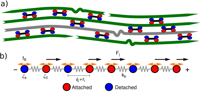
Figure 1: Sketch of the active single-chain model with Brownian forces. a) Active bundle formed by polar filaments and motors (which can move towards the barbed end of the filaments). Motors attach and detach from the filaments. After detaching from a given filament a motor will step forward in that filament and will exert a force on the other filament where it is still attached. The gray filament indicates a probe filament whose dynamics are followed by the model. b) The probe filament is represented by a bead-spring chain. Red beads represent attachment sites in the filament where a motor is attached, $\zeta_{a}$ is the friction coefficient of those beads. Blue beads represent sites in the filaments where no motor is attached $\zeta_{d}$ is the friction coefficient of those beads. The orange double-headed arrows represent the Brownian forces, $f_{\rm B}$, acting on the beads. $F_{j}$ is a motor-generated force acting on bead $j$. Motors generate a force on the filament only when attached. $\ell_{0}$ is the rest length of the strands before addition of ATP; $r_{i}$ is the change in the end-to-end distance of a strand due to Brownian and motor-generated forces.

The attachment state is represented by a single number $s$; by allocating number $0$ to free sites and $1$ to sites attached to a motor. In the following, the number $0$ or $1$ assigned to site $j$ on a filament in an attachment state $s$ is denoted by $n_{j}(s)$. By definition, $s$ takes one of the values $0,1,...,2^{N}(=s_{\rm max})$, where $N$ is the total number of sites in the probe filament. The network strands have contour length $\ell_{c}$, therefore a filament has total contour length length $\ell_{f}=(N-1)\ell_{c}$. Before addition of ATP all the motor clusters are attached (as passive cross-links) and the strands between them have relaxed end-to-end length $\ell_{0}$. This is the rest length of the filament segments and therefore there is no tension in the filaments before addition of ATP. For instance, if an actin network is formed in the presence of high concentrations of myosin the resulting cross-link density is higher and $\ell_{0}$ smaller than in the same network formed under lower concentrations. In typical actin networks prepared in vitro $\ell_{0}$ is on the order of $1\leavevmode\nobreak\ \mu$m ⁶, ⁷. The average time a motor spends attached to a site before detaching from it is labeled $\tau_{d}$, whereas the average time a motor spends detached before reattaching is given by the model parameter $\tau_{a}$. The force generated by a motor attached to site $j$ will be denoted $F_{j}$. Molecular motors can only move in one direction along the filament, determined by the filament’s polarity. Filaments are thus expected to move in the opposite direction. In this single-chain description this is described by making all the forces $F_{j}$, that the motors exert on the sites of the probe filament, have the same sign (either positive or negative).

Another force acting on the filament is the viscous drag from the surrounding solvent. The frictional force from the surrounding solvent is characterized by a friction coefficient. Motor clusters (i.e.: $1.5\mu$m for myosin II thick filaments) increase the friction coefficient of the filament when attached to an active site. Therefore this friction coefficient is allowed to take two different values: $\zeta_{a}$ when attached, and $\zeta_{d}<\zeta_{a}$ if there is no motor attached to that site.

In summary the following state variables are used to construct the model of the active gel $\Omega:\{s,\bm{F},\bm{r}\}$. Where $\bm{F}:=\{F_{1},F_{2},F_{j},...F_{N}\}$ is a vector that contains the motor forces for all the sites and $\bm{r}:=\{r_{1},r_{2},r_{i},...r_{N-1}\}$ is a vector that contains the change from the rest length in the end-to end distance of all the strands. Now let $\psi(\Omega)$ be the distribution function describing the probability of finding an active filament in state $s$ with strands with a change in their end-to-end distance $\bm{r}$ due to motor forces $\bm{F}$ at time $t$. The time evolution for $\psi(\Omega)$ is given by the following differential Chapman-Kolmogorov equation:

$$\frac{\partial\psi(\hat{\omega},\bm{r};t)}{\partial t} = \sum_{i,j=1}^{N-1}\frac{\partial}{\partial r_{i}}\bigg{\{}\psi(\hat{\omega},\bm{r};t)\bigg{[}-\dot{\epsilon}(t)r_{j}+A_{i,j}(s)f(r_{j})-\frac{\left(F_{j+1}-F_{j}\right)\delta_{i,j}}{\zeta_{a}}\bigg{]}$$

$$+ A_{i,j}(s)k_{\rm B}T\dfrac{\partial\psi(\hat{\omega},\bm{r};t)}{\partial r_{j}}\bigg{\}}+\sum_{s^{\prime}=0}^{s_{\rm max}}\int\mathbb{W}_{s,s^{\prime}}(\hat{\omega}|\hat{\omega}^{\prime})\psi(\hat{\omega}^{\prime},\bm{r};t)d\bm{F}^{\prime}$$

where $\hat{\omega}:\{s,\bm{F}\}$ is a subspace of $\Omega$, $\epsilon(t)$ is an externally applied strain and $f(r_{j})$ is the spring force. The term proportional to $k_{\rm B}T$, which introduces the effect of Brownian forces, differentiates this model from previous versions of the active single-chain model which did not include it ²⁰, ²¹.

For the Fraenkel springs considered here $f(r_{j})=-k_{b}r_{j}$. The linear spring constant for inextensible (ie.: fixed contour length $\ell_{c}$) semiflexible filaments ²⁶ is given by $k_{b}=\dfrac{90k_{\rm B}T\ell^{2}_{p}}{\ell_{0}^{4}}$. The rest length $\ell_{0}$ is related to the contour length by $\ell_{0}=\ell_{c}-\dfrac{\ell_{0}^{2}}{6\ell_{p}}$. For F-actin filaments, the persistence length, $\ell_{p}$, is approximately 10 $\mu$m and $\ell_{0}\sim 1\mu$m and therefore $k_{b}$ is on the order of $1\leavevmode\nobreak\ \mu$N/m. The matrix $A_{i,j}(s)$, in eq.(2.1) gives the connectivity of the sites as a function of the motor-attachment state, $s$, and is defined as,

$$A_{i,j}(s)=-a_{i}(s)\delta_{i,j-1}+[a_{i}(s)+b_{i}(s)]\delta_{i,j}-b_{i}(s)\delta_{i,j+1}$$ (2)

where $a_{i}(s)$ and $b_{i}(s)$ are given by,

$$\left\{a_{i}(s),b_{i}(s)\right\}=\left\{\begin{array}[]{lll}\left\{\frac{1}{\zeta_{a}},\frac{1}{\zeta_{a}}\right\}&{\rm if}&\{n_{i}(s),n_{i+1}(s)\}=\{1,1\}\\ \left\{\frac{1}{\zeta_{d}},\frac{1}{\zeta_{a}}\right\}&{\rm if}&\{n_{i}(s),n_{i+1}(s)\}=\{0,1\}\\ \left\{\frac{1}{\zeta_{a}},\frac{1}{\zeta_{d}}\right\}&{\rm if}&\{n_{i}(s),n_{i+1}(s)\}=\{1,0\}\\ \left\{\frac{1}{\zeta_{d}},\frac{1}{\zeta_{d}}\right\}&{\rm if}&\{n_{i}(s),n_{i+1}(s)\}=\{0,0\}.\\ \end{array}\right.$$ (7)

As stated above, $\zeta_{a}$ is the friction coefficient of a site when a motor is attached to it and $\zeta_{d}$ is the friction coefficient when there is no motor attached to the site.

The transition rate matrix $\mathbb{W}(\hat{\omega}^{\prime}|\hat{\omega})$ in eq.(2.1) contains the transition rates between attachment/detachment states. To construct $\mathbb{W}(\hat{\omega}^{\prime}|\hat{\omega})$ a matrix $\mathbb{K}(l)$ of dimensions $2^{l}\times 2^{l}(l=1,...,N)$ is first generated by the following iterative procedure:

$$\mathbb{K}(l)=\left(\begin{array}[]{cc}\mathbb{K}(l-1)&\dfrac{1}{\tau_{d}}\prod_{i=1}^{N}\delta(F_{i}^{\prime})\bm{\delta}(2^{l-1})\\ \dfrac{p(F_{l}^{\prime})}{\tau_{a}}\prod_{(i\neq l)=1}^{N}\delta(F_{i}^{\prime})\bm{\delta}(2^{l-1})&\mathbb{K}(l-1)\end{array}\right).$$ (10)

Where $\mathbb{K}(0)=1$, $\delta(...)$ is the Dirac delta function and $\bm{\delta}(2^{l})$ is an identity matrix of dimensions $2^{l}\times 2^{l}$. Then $\mathbb{W}(\hat{\omega}^{\prime}|\hat{\omega})$ is defined in terms of $\mathbb{K}(l)$ as,

$$\mathbb{W}(\hat{\omega}^{\prime}|\hat{\omega})=\left\{\begin{array}[]{lll}\mathbb{K}_{s^{\prime},s}(N)&{\rm if}&s^{\prime}\neq s\\ -\sum_{s^{\prime\prime}(\neq s)=0}^{s_{\rm max}}\mathbb{K}_{s^{\prime\prime},s}(N)&{\rm if}&s=s^{\prime}.\end{array}\right.$$ (13)

The block matrix at the upper-left or lower-right block element of $\mathbb{W}(\hat{\omega}^{\prime}|\hat{\omega})$ represents the transition rate matrix of a chain having $N-1$ sites, whereas the upper right and lower left elements stand for the detachment and attachment rates of motors in the $Nth$ site, respectively. In the strong attachment case, when $\tau_{a}\ll\tau_{d}$, a good approximation is to consider only attachment states with a maximum of one detached motor ²⁷. This reduces the size of the transition matrix from $2^{N}\times 2^{N}$ to $(N+1)\times(N+1)$. This approximation can make numerical simulations of the model more efficient. Explicit forms of the transition matrices for $N=2$ and $N=3$ that illustrate this point are given in a Supplementary Information file. In actomyosin gels ²⁸ the typical value for the ratio $\tau_{a}/\tau_{d}$ lies around $0.005$. In this work the strong attachment approximation was employed in all the numerical simulations of the model where $\tau_{a}/\tau_{d}<0.05$.

The function $p(F)$ is the probability distribution from which a motor force is drawn every time a motor attaches to a site. Motor force distributions have been measured experimentally in actomyosin bundles ^{29, 28}. In order to obtain analytic solutions of the model it is necessary to assume that the motor force distribution is given by a Dirac delta function centered around the mean-motor stall force that is $p(F)=\delta(F-F_{m})$. where $F_{m}$ is the mean motor-stall force. A more realistic shape of these motor force distributions can be incorporated into the model. For instance, the shape of the cumulative probability function of myosin motor forces in actin bundles appears to follow a gamma distribution ²⁹, ²¹. Therefore to incorporate a more realistic distribution of motor forces in the model a fit of a gamma distribution to the experimental data in actomysoin bundles ²⁹ is used. The fit to the experimental data has been shown in a previous paper ²¹ and results in a gamma distribution with scale parameter $\beta=0.42F_{m}$ and shape parameter of $\alpha=F_{m}/\beta=2.4$.

It was previously shown that closed-form analytic solutions to the active single-chain model can be obtain in certain simplified cases ²⁰. To perform numerical simulations of the proposed model is more convenient to write the dynamics in phase space instead of the configuration space given by the Chapman-Kolmogorov equation. For the model with Brownian forces, the evolution equations for the filament segments in the phase space are given by the following stochastic differential equations,

$$dr_{i,s} = \dot{\epsilon}r_{i,s}dt-\sum_{j=1}^{N-1}\left\{A_{i,j}(s)f(r_{j,s})-\frac{\left[F_{j+1}-F_{j}\right]\delta_{i,j}}{\zeta_{a}}\right\}dt$$

$$+ \sqrt{2k_{\rm B}T}\sum_{j=1}^{N-1}B_{i,j}(s)dW_{j}(t),(i=1,2,3,...,N-1).$$

Where $dW(t)$ is a Wiener increment with statistics, $\left\langle{dW}_{i}(t)\right\rangle_{\rm eq}=0$ and $\left\langle{dW}_{i}(t){dW}_{j}(t^{\prime})\right\rangle_{\rm eq}=\delta(t-t^{\prime})\delta_{ij}dtdt^{\prime}$. On the other hand the matrix $\bm{B}(s)$ must satisfy, $[\bm{B}(s)]\cdot[\bm{B}(s)]^{\top}=\bm{A}(s)$ which guarantees that the Brownian forces satisfy the fluctuation dissipation theorem. An efficient way to construct the matrix $\bm{B}$ is,

$$B_{i,j}(s)=\left\{\begin{array}[]{ccc}-\sqrt{2k_{\rm B}Ta_{i}(s)}&{\rm if}&i=j\\ \sqrt{2k_{\rm B}Tb_{i}(s)}&{\rm if}&i+1=j\\ 0&{\rm elsewhere}&\\ \end{array}\right.$$ (18)

Where $a_{i}(s)$ and $b_{i}(s)$ where defined in eq. (7). The evolution equation for the state variables $s$ and $\bm{F}$ can be obtained by integrating eq. (2.1) over $\bm{r}$,

$$\frac{\partial\phi(\hat{\omega};t)}{\partial t}=\sum_{s^{\prime}=0}^{s_{\rm max}}\int\mathbb{W}_{s,s^{\prime}}(\hat{\omega}|\hat{\omega}^{\prime})\phi(\hat{\omega}^{\prime};t)d\bm{F}^{\prime}$$ (19)

where $\phi(\hat{\omega};t):=\int\psi(\hat{\omega},\bm{r};t)d\bm{r}$.

In a numerical simulation of the model, in every time step the probability of jumping from a given attachment state to a a new one is calculated as $p=1-\exp\left\{-\Delta t\sum_{s=0}^{s_{\rm max}}\sum_{s^{\prime}(\neq s)=0}^{s_{\rm max}}\mathbb{W}_{s,s^{\prime}}\right\}$. The time step of the simulation, $\Delta t$, is chosen such that $\Delta t<1/\sum_{s=0}^{s_{\rm max}}\sum_{s^{\prime}(\neq s)=0}^{s_{\rm max}}\mathbb{W}_{s,s^{\prime}}$, $\Delta t\ll\tau_{r,a}$ and $\Delta t\ll\tau_{r,d}$, where $\tau_{r,a}=\zeta_{a}/k_{b}$ and $\tau_{r,d}=\zeta_{d}/k_{b}$. If a jump is accepted then the probabilities of a filament that is in attachment state $s^{\prime}$ to jump to attachment state $s$ are calculated according to the transition matrix $\mathbb{W}_{s,s^{\prime}}$. If the larger probabilities correspond to states that require a detachment then one of those states is chosen randomly, the transition occurs, and the respective motor forces, $F_{j}$, are set to zero. If the larger probabilities correspond to states that require an attachment then random motor forces are generated from a gamma distribution. Then the probability for each of those generated forces is calculated from the gamma probability density function and the state with the highest probability is chosen.

2.2 Mass transport

The diffusion of tracer beads or labeled filaments inside active gels has been studied both experimentally and theoretically ^{30, 31, 14}. The mass transport of microscopic probe particles in active gels has been observed to exhibit super-diffusive behavior at time scales at which in passive polymeric networks probe particles exhibit diffusive behavior ^{30, 14, 17}. For example, the mean-squared displacement, MSD, of microscopic tracer particles embedded in microtubules and kinesin solutions for increasing ATP concentrations from 0 to 5.6 mM has been reported ¹⁷. At ATP concentrations above 73 $\mu$M the the MSD exhibits ballistic behavior at all lag times measured, from $10^{-1}$ to $10^{3}$ seconds. MSDs of endogenous particles inside the cytoplasm of live and motile Amoeba proteus ¹⁸ have also been reported. In that system, the MSD exhibits either diffusive or super-diffusive regions at lag times above $\sim 3$ ms , depending on the location, inside the amoeba, of the tracked particle. Moreover, Head et al. ³² have also investigated the mass-transport of filaments in active gels using a multi-chain simulation of an active gel. They found that filament translational motion ranges from diffusive to super-diffusive, depending on the ratio of attachment/detachment rates of the motors ³².

In the active single-chain model the mass transport of filaments inside and active gel can be quantified by the mean-squared displacement of a probe filament’s center of mass, $\langle\Delta R_{c}^{2}(t)\rangle_{\rm st}=\langle[r_{\rm cm}(t)-r_{\rm cm}(0)]^{2}\rangle_{\rm st}$. Figure 2A shows the $\langle\Delta R^{2}(t)\rangle_{\rm st}$ of a filament with four motor attachment sites, $N=4$, for different ratios of motor to Brownian forces, ranging from a highly active gel, $\dfrac{F_{m}\ell_{c}}{k_{\rm B}T}=100$, to a mostly passive gel, $\dfrac{F_{m}\ell_{c}}{k_{\rm B}T}=0.01$. For this lowest ratio between motor and Brownian forces the $\langle\Delta R^{2}(t)\rangle_{\rm st}$ exhibits diffusive behavior, $\sim t^{n\sim 1}$, at all the time scales sampled. For $\dfrac{F_{m}\ell_{c}}{k_{\rm B}T}=0.1$ apparent diffusive behavior, is also observed up to $t\lesssim\tau_{d}$ but super-diffusive behavior ($\sim t^{n>1}$) can be seen at longer times, $t>10\tau_{d}$. When $\dfrac{F_{m}\ell_{c}}{k_{\rm B}T}=1$ the diffusive region becomes much shorter and super-diffusive mass transport can be observed at time scales as short as $t\sim 10^{-2}\tau_{d}$. For gels with ratios of motor to Brownian forces higher than one the $\langle\Delta R^{2}(t)\rangle_{\rm st}$ behaves ballistic, $\sim t^{2}$, at all the lag times sampled. The results show that, as expected, a probe filament will undergo diffusive motion in the gel due to Brownian forces, as the magnitude of motor-generated forces becomes larger their pulling on the filament becomes increasingly important and at long times they are able to effectively accelerate the motion of the filament’s center of mass. For low ratios between motor and Brownian forces the latter are still able to counteract, at short times, the directional pulling of the motors with the Brownian motion of the filament segments. For large ratios between motor and Brownian forces the latter can not longer counteract the pulling done by the motor forces at any of the observable time scales.

\begin{overpic}[width=208.13574pt]{./fig1A.eps} \put(18.0,80.0){\small(A)} \end{overpic}

\begin{overpic}[width=208.13574pt]{./fig1B.eps} \put(18.0,80.0){\small(B)} \end{overpic}

Figure 2: Steady state mean squared displacement of a filament in the active single-chain model with $N=4$ as a function of A) the ratio between motor and Brownian forces with $\tau_{a}/\tau_{d}=0.005$, and B) the ratio between attachment time and detachment time of the motor clusters for $\dfrac{F_{m}\ell_{c}}{k_{\rm B}T}=10.0$. The other parameters used in these calculations were set to, $\dfrac{\zeta_{a}\ell_{c}^{2}}{\tau_{d}k_{\rm B}T}=192.1$, $\zeta_{d}/\zeta_{a}=0.1$, $\ell_{p}/\ell_{c}=10$.

Figure 2B shows the $\langle\Delta R^{2}(t)\rangle_{\rm st}$ for different ratios of motor detachment time, $\tau_{d}$, to attachment time, $\tau_{a}$, for a fixed value of the ratio between motor and Brownian forces, $\dfrac{F_{m}\ell_{c}}{k_{\rm B}T}=10$. For the two highest $\tau_{a}/\tau_{d}$ ratios, 500 and 100, the behavior of the $\langle\Delta R^{2}(t)\rangle_{\rm st}$ is ballistic at short time scales, $t\lesssim 10^{-2}\tau_{d}$, and diffusive at longer time scales. This indicates that for these cases the motor attachment times, $\tau_{a}$, are too long compared to the relaxation times of the filament segments. Since the filaments segments have enough time to relax between motor attachment events the motor proteins are not able to maintain the acceleration of the center of mass of the filaments at long times. For the lowest $\tau_{a}/\tau_{d}$ ratios, 1.0 and 0.005, no significant local relaxation can occur in the filament segments between motor attachment events and the behavior of $\langle\Delta R^{2}(t)\rangle_{\rm st}$ is super-diffusive at all the observable lag times. These results indicate that even for a very active gel, where motor forces dominate over Brownian forces, the mass transport of filaments will only exhibit super-diffusive behavior at low $\tau_{a}/\tau_{d}$ ratios, when the motors spend enough time pulling on the filaments and are able to accelerate their motion. These dependence of the $\langle\Delta R^{2}(t)\rangle_{\rm st}$ on $\tau_{a}/\tau_{d}$ is in agreement with what was observed in the active single-chain model that did not include Brownian forces ²¹. In that model as well for gels with weak motor attachment, large $\tau_{a}/\tau_{d}$ ratios, the motion of the filaments has two well-defined regions. At short time scales, shorter than $\tau_{d}$, the $\langle\Delta R^{2}(t)\rangle_{\rm st}$ goes as $\sim t^{2}$. While for larger time scales the behavior becomes diffusive. For strong attachment cases, small $\tau_{a}/\tau_{d}$ ratios, the $\langle\Delta R^{2}(t)\rangle_{\rm st}$ of the model without Brownian forces also exhibited ballistic behavior at all time scales.

2.3 Dynamic Modulus

To test the validity of FDT in active gels Mizuno et al. ¹⁶ compared the complex compliance of actomyosin networks measured with driven and passive probe particle microrheology. In the driven experiment an optical trap is used to apply a small-amplitude oscillatory force, $\bm{f}^{\rm trap}$, with a frequency $\omega$ to the probe particle. The complex compliance, $\alpha(\omega)$, is obtained form the relation $\bm{r}_{\rm b}(\omega)=\alpha(\omega)\bm{f}^{\rm trap}$, where $\bm{r}_{\rm b}(\omega)$ is the measured bead position at steady state. In a passive microrheology experiment no external force is applied to the bead or a static harmonic trap is used to hold the bead near its steady state position and the imaginary part of $\alpha(\omega)$ is obtained using the FDT, $\alpha^{\prime\prime}(\omega)=\dfrac{\omega}{6k_{\rm B}T}C(\omega)$. Where $C(\omega)=\int_{-\infty}^{\infty}\langle\bm{r}_{\rm b}(t)\cdot\bm{r}_{\rm b}(0)\rangle e^{-i\omega t}dt$ is the autocorrelation function of the bead position. Note also that, the complex compliance of the probe particle can be related to the creep compliance of the material by using a generalized Stokes relation, $J^{\prime\prime}(\omega)=6\pi R\alpha^{\prime\prime}(\omega)$. Before addition of ATP the complex compliance of the actomyosin networks obtained with the passive and driven microrheology experiments have been observed to agree. When the gels are activated with ATP a discrepancy is observed between the complex compliance obtained from the passive and driven microrheology experiments. This discrepancy appears at frequencies below 10 Hz and becomes larger with decreasing frequency.

\begin{overpic}[width=208.13574pt]{./fig2A.eps} \put(18.0,72.0){\small(A)} \end{overpic}

\begin{overpic}[width=208.13574pt]{./fig2B.eps} \put(18.0,73.0){\small(B)} \end{overpic}

Figure 3: (A) Storage moduli of the active single-chain dumbbell model, $N=2$, and Dirac delta motor force distribution, $p(F)=\delta(F-F_{m})$ for different values of the ratio between motor and Brownian forces. The other parameters used in these calculations were set to, $\dfrac{\zeta_{a}\ell_{c}^{2}}{\tau_{d}k_{\rm B}T}=192.1$, $\zeta_{d}/\zeta_{a}=0.1$, $\tau_{a}/\tau_{d}=0.005$, $\ell_{p}/\ell_{c}=10$. The inset shows the storage modulus for the active single-chain dumbbell model without Brownian forces with $p(F)=\delta(F-F_{m})$, $\zeta_{a}/k_{b}=0.02$, $\zeta_{d}/\zeta_{a}=0.1$ and $\tau_{a}/\tau_{d}=0.005$. The continuous lines correspond to Green-Kubo calculations and the dashed lines to driven calculations. (B) Check of the fluctuation dissipation theorem in the systems shown in part (A).

In previous work ²⁰, ²¹ it was shown that the active single-chain model without Brownian forces is able to describe the violation of the FDT observed in microrheology experiments in active gels. Here the active single-chain model with Brownian forces will be tested in the same way. To do this the relaxation modulus of the active gel is calculated by two different methods. In one method no external strain is applied, $\dot{\epsilon}(t)=0$ in eq.(2.1), and the Green-Kubo formula is used to calculate the relaxation modulus of the material from the autocorrelation function of stress at steady state ²¹, $G_{\rm GK}(t)=\dfrac{1}{n_{c}k_{\rm B}T}\left\langle\sigma(t)\sigma(0)\right\rangle_{\rm{st}}$. For a mean-field single-chain model, like the one employed here, the macroscopic stress, $\sigma$, is related to the tension on the filaments by $\sigma=-n_{c}\sum_{i=1}^{N-1}f_{i}r_{i}$ where $f_{i}$ is the tension on a filament segment and $n_{c}$ is the number of filaments per unit volume ^{27, 33, 34}. For calculations with Fraenkel springs the macroscopic stress simplifies to $\sigma=n_{c}k_{b}\sum_{i=1}^{N-1}r_{i}^{2}$. The non-equilibrium steady state dynamic modulus of the active gel can then be obtained by taking the one-sided Fourier transform of the relaxation modulus, $G^{*}(\omega)=i\omega\bar{\mathcal{F}}\{G(t)\}=G^{\prime}(\omega)+iG^{\prime\prime}(\omega)$. Where $\bar{\mathcal{F}}\{G(t)\}:=\int_{0}^{\infty}G(t)e^{-i\omega t}dt$ is the one-sided Fourier transform; $G^{\prime}(\omega)$ is the storage modulus and $G^{\prime\prime}(\omega)$ is the loss modulus. In a second calculation, the dynamic modulus is obtained from the stress response to an externally applied small-amplitude oscillatory strain or from a small step strain. For the dumbbell version of the model, $N=2$, and a Dirac delta motor force distribution, $p(F)=\delta(F-F_{m})$, these two calculations can be carried out analytically. The details of the analytical procedure to derive the dynamic modulus from these two types of calculations has been presented elsewhere ²⁰.

Figure 3A shows the storage modulus for the dumbbell version of the active single-chain model with a Dirac delta motor force distribution for different ratios of motor to Brownian forces. Note that for the dumbbell case, the gel is formed by filaments of length $\ell_{c}$ with only two motor attachment sites per filament. Again, to relate the model predictions to experimental observations it will be considered that the the ratio of motor to Brownian forces is proportional to the concentration of ATP in the active gel. Higher ATP concentrations yield higher motor to Brownian forces ratios while ATP-depleted gels have lower motor to Brownian forces ratios. Figure 3B shows the same type of frequency dependent violation of the FDT that was previously observed with the model that did not include Brownian forces. The modulus obtained from the Green-Kubo formula and the modulus obtained from the driven calculation agree at high frequency, but diverge at low frequencies. Moreover, this discrepancy at low frequencies becomes larger with increasing ratio between motor and Brownian forces. For the higher ratios between motor and Brownian forces a maximum appears in the storage moduli obtained from the Green-Kubo formula at frequencies around $10^{2}/\tau_{d}$. This feature of the dynamic modulus of active gels had already been observed before in the version of the model without Brownian forces ²⁰ and is also seen here for large ratios of motor to Brownian forces. For comparison, the storage modulus of the active single-chain model without Brownian forces is shown in the inset of Figure 3A. Note that this modulus has been calculated with parameters that are equivalent to the ones used for the model with Brownian forces. That is, $\zeta_{a}/k_{b}=0.02$, $\zeta_{d}/\zeta_{a}=0.1$ and $\tau_{a}/\tau_{d}=0.005$. Also important is that in the limit of very small ratios of motor to Brownian forces the modulus from the passive calculation agrees exactly with the modulus from the active calculation at all frequencies and the FDT is recovered (Figure 3B), as expected for a passive polymer network.

\begin{overpic}[width=208.13574pt]{./fig3A.eps} \put(18.0,72.0){\small(A)} \end{overpic}

\begin{overpic}[width=208.13574pt]{./fig3B.eps} \put(18.0,72.0){\small(B)} \end{overpic}

Figure 4: (A) Relaxation moduli, calculated with the Green-Kubo formula, of the active single-chain model with $N=4$ and for different values of the ratio between motor and Brownian forces. The symbols are simulation results and the lines are fits to a multimode Maxwell model used to transfer the information to the frequency domain. The other parameters used in these calculations were set to, $\dfrac{\zeta_{a}\ell_{c}^{2}}{\tau_{d}k_{\rm B}T}=192.1$, $\zeta_{d}/\zeta_{a}=0.1$, $\tau_{a}/\tau_{d}=0.005$, $\ell_{p}/\ell_{c}=10$. Here and below the error bars on the autocorrelation of stress, $G_{\rm GK}(t)$, were calculated using the “blocking transformations” method, which accounts for the correlation in the time-series data ³⁵. (B) Dynamic modulus of the active single-chain model calculated from the relaxation moduli shown in part (A). The continuous lines correspond to the storage moduli, $G^{\prime}$, and the dashed lines to the loss moduli, $G^{\prime\prime}$.

The inclusion of Brownian forces in the model also introduces additional features in the shape of the storage modulus that are not observed in the dumbbell version of the model without Brownian forces. In particular, a scaling of $G^{\prime}\sim\omega^{0.5}$ appears at intermediate frequencies, $2\times 10^{2}\lesssim\omega\tau_{d}\lesssim 10^{4}$ , for the lower motor to Brownian forces ratios. This stress relaxation mechanisms is of the Rouse type and is also observed in temporary networks formed by associating polymers ^{27, 36}, where it is called associative Rouse behavior, to distinguish it from another Rouse relaxation region observed at high frequencies in those gels. For the active single-chain model with Brownian forces, the Rouse behavior appears in the frequency region bounded by $\tau_{r,a}=\zeta_{a}/k_{b}=0.02\tau_{d}$, and $\tau_{r,d}=\zeta_{d}/k_{b}=0.002\tau_{d}$. In the active single-chain model without Brownian forces this type of behavior is not observed for dumbbells (see inset of Figure 3A) and only appeared for longer filaments where the longest relaxation time of the gel becomes significantly larger than $\tau_{d}$. Here, however this relaxation mode is observed at time scales between three and two orders of magnitude smaller than $\tau_{d}$. This indicates that Brownian forces introduce faster relaxation dynamics that were not present in the model without Brownian forces. However final conclusions should not be drawn from the dynamics of the dumbbell versions of the model since these are unrealistically fast. More realistic systems, that require numerical solutions of the model, will be addressed below. Still the analytic calculations that can be performed with the dumbbell model provide a good reference point for the more complex numerical simulations.

In Figure 4A the relaxation moduli for gels formed by filaments of length $\ell_{t}=3\ell_{c}$, or equivalently filaments with $N=4$, and for five different ratios of motor to Brownian forces are shown. In Figure 4B the corresponding dynamic moduli are presented. For these calculations the motor forces were generated from a gamma distribution with scale parameter $\beta=0.42F_{m}$. Note that when the mean motor stall force, $F_{m}$, is varied the shape parameter of the gamma distribution, $\alpha=F_{m}/\beta=2.4$, remains constant. These shape and scale parameters were obtained by fitting a a gamma probability distribution to a motor force distribution measured in actomyosin bundles ²⁹. As expected, with these longer filaments and the more realistic motor force distribution a broader spectrum of relaxation times can be observed compared to the results for the dumbbell filaments. For the lowest ratio between motor and Brownian forces, $\dfrac{F_{m}\ell_{c}}{k_{\rm B}T}=1.0$, the dynamic modulus has the shape typically observed in temporary polymeric networks. A cross-over between $G^{\prime}$ and $G^{\prime\prime}$, which is associated with the longest relaxation time of the network is observed at frequencies around $10^{2}/\tau_{d}$. Below this frequencies the terminal zone of stress relaxation is observed with $G^{\prime}\sim\omega^{2}$ and $G^{\prime\prime}\sim\omega$. At high frequencies $G^{\prime}$ exhibits a plateau region.

As the ratio of motor to Brownian forces is increased the magnitude and shape of $G_{\rm GK}(t)$ and therefore of $G^{*}_{\rm GK}$ change significantly. These changes are more pronounced at low frequencies, below $10^{2}/\tau_{d}$, where new or additional local maxima appear both in $G^{\prime}$ and $G^{\prime\prime}$. For a ratio of motor to Brownian forces of $\dfrac{F_{m}\ell_{c}}{k_{\rm B}T}=70$ new features in $G^{\prime}$ and $G^{\prime\prime}$ are observed around $1/\tau_{d}\lesssim\omega\lesssim 10^{2}/\tau_{d}$. Moreover the crossover between $G^{\prime}$ and $G^{\prime\prime}$ is slightly displaced to lower frequencies. As the ratio between motor and Brownian forces is increased the overall magnitude of $G^{*}_{\rm GK}$ increases further, the size of the low-frequency peaks in $G^{\prime\prime}$ also increases and the crossover frequency between $G^{\prime}$ and $G^{\prime\prime}$ moves to even lower frequencies. In particular, this last observation indicates that a $200$ fold increase in the ratio between motor and Brownian forces will increase the longest relaxation time of the gel by two orders of magnitude. Note that in the model with Brownian forces $G^{\prime\prime}$ always exhibits two maxima, a low frequency one around the crossover and one at higher frequencies. The one at higher frequencies was not observed in the model without Brownian forces.

\begin{overpic}[width=208.13574pt]{./fig4A.eps} \put(18.0,72.0){\small(A)} \end{overpic}

\begin{overpic}[width=208.13574pt]{./fig4B.eps} \put(18.0,72.0){\small(B)} \end{overpic}

Figure 5: (A) Relaxation moduli, calculated with the Green-Kubo formula, of the active single-chain model with $N=8$ and for different values of the ratio between motor and Brownian forces. The symbols are simulation results and the lines are fits to a multimode Maxwell model used to transfer the information to the frequency domain. The other parameters used in these calculations were set to, $\dfrac{\zeta_{a}\ell_{c}^{2}}{\tau_{d}k_{\rm B}T}=192.1$, $\zeta_{d}/\zeta_{a}=0.1$, $\tau_{a}/\tau_{d}=0.005$, $\ell_{p}/\ell_{c}=10$. (B) Dynamic modulus of the active single-chain model calculated from the relaxation moduli shown in part (A). The continuous lines correspond to the storage moduli, $G^{\prime}$, and the dashed lines to the loss moduli, $G^{\prime\prime}$.

Figure 5 illustrates the effect on $G_{\rm GK}(t)$ and $G^{*}_{\rm GK}$ when the filament length is increased to $\ell_{t}=7\ell_{c}$, or equivalently filaments with $N=8$. The gel formed by these even longer filaments and with $\dfrac{F_{m}\ell_{c}}{k_{\rm B}T}=1$ exhibits a longer power law relaxation mode, $G^{\prime}\sim\omega^{1/2}$ at frequencies near the crossover between $G^{\prime}$ and $G^{\prime\prime}$. Moreover, this crossover is also shifted to lower frequencies, as expected for gels formed by higher molecular weight filaments. As the ratio between motor and Brownian forces is increased the magnitudes of $G_{\rm GK}(t)$ and $G^{*}_{\rm GK}$ also increase significantly. Also, the longest relaxation time increases by two orders of magnitude when the ratio between motor forces and Brownian forces is increased by a factor of 200. The low frequency maxima are still present for both $G^{\prime}$ and $G^{\prime\prime}$. However, for these longer filaments the maximum in $G^{\prime\prime}$ that appeared at higher frequencies, $\omega\sim 10^{2}/\tau_{d}$, is very small which seems to indicate that it will tend to disappear as the filaments are made longer.

\begin{overpic}[width=208.13574pt]{./fig5A.eps} \put(18.0,72.0){\small(A)} \end{overpic}

\begin{overpic}[width=208.13574pt]{./fig5B.eps} \put(18.0,72.0){\small(B)} \end{overpic}

Figure 6: (A) Dynamic moduli of the active single-chain model with $\dfrac{F_{m}\ell_{c}}{k_{\rm B}T}=1$ calculated from Green-Kubo simulations for different values of the filament length, $\ell_{t}=(N-1)\ell_{c}$. (B) Dynamic moduli of the active single-chain model with $\dfrac{F_{m}\ell_{c}}{k_{\rm B}T}=70$ calculated from Green-Kubo simulations for different values of the filament length, $\ell_{t}=(N-1)\ell_{c}$. The other parameters used in these calculations were set to, $\dfrac{\zeta_{a}\ell_{c}^{2}}{\tau_{d}k_{\rm B}T}=192.1$, $\zeta_{d}/\zeta_{a}=0.1$, $\tau_{a}/\tau_{d}=0.005$, $\ell_{p}/\ell_{c}=10$. The continuous lines correspond to the storage moduli, $G^{\prime}$, and the dashed lines to the loss moduli, $G^{\prime\prime}$.

Note that the associative Rouse relaxation mode, $G^{\prime}\sim\omega^{1/2}$, observed in the calculations with the active single-chain model is a result of the simplified description of the polymeric filaments. In the active single-chain model the filament segments are described by Fraenkel springs. However, real semiflexible filaments have finite-extensibility and the tension in a particular segment is strongly coupled to the orientation of the other segments in the filament. The effect of finite-extensibility in the rheology of active gels was previously addressed using the active single-chain model without Brownian forces ²¹. Moreover, a more accurate bead-spring chain discretization of the semiflexible filaments should also include bending potentials between the springs which introduce correlations between the orientations of the filament segments ^{37, 38}.

To illustrate how the stress relaxation dynamics in active gels behave for even longer filaments Figure 6 shows a comparisons between the dynamic moduli of filaments with $N=4$, $N=8$ and $N=20$ for ratios of motor to Brownian forces, $\dfrac{F_{m}\ell_{c}}{k_{\rm B}T}=1$ and $\dfrac{F_{m}\ell_{c}}{k_{\rm B}T}=70$. Note that for the gels with the lower ratio between motor and Brownian forces increasing the filament length by a factor of about five increases the longest relaxation time by two orders of magnitude. Moreover, the breadth of the Rouse-type low-frequency relaxation mechanism, $G^{\prime}\sim\omega^{1/2}$, increases from one decade to three decades of frequency when the filament length increases by a factor of about five. Also as expected, gels formed by longer filaments exhibit dynamic moduli with overall higher magnitude. For the gels with $\dfrac{F_{m}\ell_{c}}{k_{\rm B}T}=70$ the crossover between $G^{\prime}$ and $G^{\prime\prime}$ moves to lower frequencies and the overall magnitude of $G^{*}_{\rm GK}$ increases as $N$ is increased. Also, for these gels with larger motor forces the low frequency peaks in $G^{\prime}$ and $G^{\prime\prime}$ become larger as $N$ is increased. For instance, for $N=4$ the low frequency peak that appears in $G^{\prime\prime}$ at $\omega\sim 1/\tau_{d}$ is small compared to the higher frequency peak that appears at $\omega\sim 10^{2}/\tau_{d}$. For $N=8$ these two peaks have similar magnitude and $G^{\prime\prime}$ exhibits a long plateau between $1/\tau_{d}\lesssim\omega\lesssim 10^{2}/\tau_{d}$. Then for $N=20$ the lower frequency peak in $G^{\prime\prime}$ becomes much larger than the higher frequency peak and a clear maximum also appears in $G^{\prime}$ at frequencies around the crossover between $G^{\prime}$ and $G^{\prime\prime}$. Note that the experimental counterpart of the Gree-Kubo simulations discussed so far are passive microrheology experiments. In the next subsection simulation results that are comparable to driven rheological experiments will be discussed.

2.4 Comparisons to microrheology experiments in actomyosin gels

To compare the active single-chain model predictions to driven microrheology experiments the relaxation modulus obtained from the stress response to an externally applied small step-strain is calculated. To do this, an ensemble of chains with dynamics given by eq.(2.1) was simulated. These simulations were started from an initial condition in which all the strands are relaxed, $r_{i}=0$ for all $i$, and then the ensemble of chains is allowed to reach steady state before applying a small step-strain of magnitude $\epsilon_{0}$, at $t=t_{\rm st}$. Simulations are performed with progressively smaller values of $\epsilon_{0}$ to check for convergence to the linear response regime. It is assumed that on the time scale of interest for which $G(t)$ is calculated the step-strain applied at the boundaries propagates instantaneously through the system. Therefore $r_{i}(t=t_{\rm st}+)=r_{i}(t=t_{\rm st}-)+\epsilon_{0}r_{i}(t=t_{\rm st}-)$ for $i=1,2,3,...,N-1$, where $\epsilon_{0}$ is the strain magnitude. Then the relaxation of stress back to its steady state value is followed. In this externally driven calculation the relaxation modulus is given by $G_{\rm D}(t)=\dfrac{\langle\sigma(t)\rangle_{\rm st}}{\epsilon_{0}}$. The subscript D indicates that the modulus is obtained from an externally driven experiment (externally applied strain). To obtain the plots shown here an average over an ensemble of $2.1\times 10^{5}$ filaments is taken. In Figure 7A the relaxation moduli as a function of the ratio between motor and Brownian forces for gels with $N=8$ are shown. For comparison, the relaxation moduli obtained from the steady state autocorrelation function of stress using the Green-Kubo formula are shown in Figure 7B. In both types of calculations the calculated relaxation modulus exhibits an overall increase in magnitude as the ratio between active and Brownian forces is increased. Also, both calculations show a slowing down of the stress relaxation dynamics as the ratio of motor to Brownian forces is increased. However, both of these effects are much more pronounced in $G_{\rm GK}(t)$ than in $G_{\rm D}(t)$.

\begin{overpic}[width=208.13574pt]{./fig6A.eps} \put(85.0,72.0){\small(A)} \end{overpic}

\begin{overpic}[width=208.13574pt]{./fig6B.eps} \put(85.0,72.0){\small(B)} \end{overpic}

Figure 7: Relaxation modulus of the active single-chain model as a function of the ratio between motor-generated and Brownian forces. The symbols are simulation results and the lines are fits to a multimode Maxwell model used to transfer the information to the frequency domain. For these calculations the parameters are set to, $N=8$, $\dfrac{\zeta_{a}\ell_{c}^{2}}{\tau_{d}k_{\rm B}T}=192.1$, $\zeta_{d}/\zeta_{a}=0.1$, $\tau_{a}/\tau_{d}=0.005$, $\ell_{p}/\ell_{c}=10$. (A) Calculated from driven step-strain simulations. (B) Calculated from the steady-state autocorrelation function of stress using the Green-Kubo formula.

To directly compare the active single-chain model predictions to available microrheology experimental data in active gels the the complex creep compliance, $J^{*}(\omega)$, needs to be computed. To contrast the model predictions to driven microrheology experiments the imaginary part of the creep compliance is calculated as $J_{\rm D}^{\prime\prime}(\omega)=\dfrac{{\rm Im}\{G^{*}_{\rm D}(\omega)\}}{|G^{*}_{\rm D}(\omega)|^{2}}$. While to compare to passive microrheology experiments the imaginary part of the creep compliance ^{30, 31} is computed as $J_{\rm GK}^{\prime\prime}(\omega)=\dfrac{{\rm Im}\{G^{*}_{\rm GK}(\omega)\}}{|G^{*}_{\rm D}(\omega)|^{2}}$. Where $G^{*}_{\rm GK}(\omega)$ is the dynamic modulus obtained from a Green Kubo simulation and $G^{*}_{\rm D}(\omega)$ is the dynamic modulus obtained from a step-strain simulation. Figure 8 shows the resulting $J^{\prime\prime}(\omega)$ obtained with the active single chain model for different values of the ratio between motor and Brownian forces. For comparison the inset shows the $J^{\prime\prime}(\omega)$ of actomyosin gels obtained from passive (squares) and driven (triangles) microrheology experiments ¹⁶. Note the characteristic frequency-dependent discrepancy between the $J^{\prime\prime}(\omega)$ obtained from passive and driven microrheology experiments. Both types of experiments agree at high frequencies but diverge at low frequencies, below 10 Hz.

At very low frequencies the model predictions do not follow the shape of the $J^{\prime\prime}(\omega)$ observed in driven microrheology experiments, while the calculated $J^{\prime\prime}$ increase with $\omega$ at low frequencies the experimental data decays with $\omega$ at low frequencies. The shape of $J^{\prime\prime}$ observed in the driven microrheology experiments is typical of polymeric gels with permanent cross-links. Therefore that particular discrepancy between the model predictions and the experimental data can be attributed to the presence of biotin cross-links in the actomyosin gels prepared by Mizuno et al ¹⁶. Besides this rather obvious discrepancy the model predictions for large ratios between motor and Brownian forces describe well the frequency dependence of $J^{\prime\prime}(\omega)$ observed in driven and passive experiments in active actomysoin gels. The model predictions show that for high motor to Brownian forces ratios $J_{\rm D}^{\prime\prime}$ and $J_{\rm GK}^{\prime\prime}$ are equal at high frequencies but the characteristic low frequency discrepancy appears around $\omega\sim 10^{2}/\tau_{d}$. For low $\dfrac{F_{m}\ell_{c}}{k_{\rm B}T}$ the low frequency difference between $J_{\rm D}^{\prime\prime}$ and $J_{\rm GK}^{\prime\prime}$ disappears which indicates that the FDT becomes valid and the gel can be regarded as passive. Is also worth comparing the predictions of the active single-chain model to the predictions of its counterpart without Brownian forces. This latter model also described correctly the low frequency discrepancy in the rheological response of active gels. However the breadth of the relaxation spectrum, especially at higher frequencies, was significantly more narrow in the model without Brownian forces. Also, the passive gel limit, where the FDT is recovered, was not attainable in the model that did not include Brownian forces. Moreover, the wider relaxation spectrum of the active single-chain model with Brownian forces represents better the observations in rheological experiments in actomyosin gels.

\begin{overpic}[width=208.13574pt]{./fig7.eps} \end{overpic}

Figure 8: The Imaginary part of the creep compliance of an active gel as a function of the ratio between motor-generated and Brownian forces calculated with the active single-chain model with Brownian forces. The dashed lines are obtained from driven step-strain simulations, while the continuous lines are obtained from Green-Kubo simulations. In all these calculations the model parameters are set to, $N=8$, $\dfrac{\zeta_{a}\ell_{c}^{2}}{\tau_{d}k_{\rm B}T}=192.1$, $\zeta_{d}/\zeta_{a}=0.1$, and $\tau_{a}/\tau_{d}=0.005$ and $\ell_{p}/\ell_{c}=10$. The inset shows the imaginary part of the creep compliance, $J^{\prime\prime}(\omega)=6\pi R\alpha^{\prime\prime}(\omega)$ observed in driven microrheology (triangles) and passive microrheology (squares) in actomyosin gels ¹⁶, where $R$ is the radius of the probe bead used in the microrheology experiments. In these particular experiments the probe particles used had $R=2.5\leavevmode\nobreak\ \mu\text{m}$.

Note that for values of $\ell_{c}\sim 2\leavevmode\nobreak\ \mu\text{m}$ and $\tau_{d}\sim 200\leavevmode\nobreak\ \text{ms}$ typical of actomyosin gels ²⁸ the friction coefficients that have been used for the model predictions throughout this work are, $\zeta_{a}\sim 0.039\leavevmode\nobreak\ \mu\rm{N\cdot s/m}$ and $\zeta_{d}\sim 0.0039\leavevmode\nobreak\ \mu\rm{N\cdot s/m}$. With these values, the Stokes relation can then be used to obtain a rough estimate the effective size of the motor clusters in the active gel. Using the viscosity of water as the solvent, $\eta\sim 10^{-3}\leavevmode\nobreak\ \rm{Pa\cdot s}$, this calculation yields a value of $\xi\equiv\dfrac{\zeta_{a}}{6\pi\eta}\sim 2\leavevmode\nobreak\ \mu$m which is consistent with the typical size of myosin motor clusters which has been reported ³ to be around $1.5\leavevmode\nobreak\ \mu$m.

3 Conclusions

The results presented here indicate that a competition between motor-generated forces and Brownian forces is important in producing characteristic features observed in the mass transport and rheological properties of active gels. Previous versions of the active single-chain model neglected Brownian forces, this simplification was assumed to be appropriate in gels with high ATP concentrations. However, the model without Brownian forces rendered only a qualitative description at ATP concentrations at which stable non-contractile in vitro active gels are prepared for rheological measurements. Is important to emphasize that no effective temperature has been introduced in the active single-chain model with Brownian forces and the motor dynamics are treated in the same way that was done in the model that did not include Brownian forces.

In this work it has been shown that the interplay between motor and Brownian forces determines the time scale for the transition from diffusive to ballistic mass transport that has been observed in microtubule solutions as ATP concentration is increased ¹⁷. Moreover it has also been shown here that the breadth of relaxation spectrum of the active single-chain model increases significantly when Brownian forces are taken into account. With respect to the predictions with the active single-chain model without Brownian forces this broadening of the relaxation spectrum occurs mostly at shorter time scales, as expected. However, for ratios between motor to Brownian forces of up to a hundred this broadening of the relaxation spectrum also has a significant influence in the shape of the dynamic modulus at lower frequencies, close to the longest relaxation time of the gel. This wider relaxation spectrum of the active single-chain model with Brownian forces represents better the observations in microrheology experiments in actomyosin gels ¹⁶.

From a practical perspective the results presented here shed light on how the rheological response of active gels changes with varying ATP concentration. Experimentally, active gels with low concentrations of ATP are usually prepared to achieve stable gels where active steady states that do not phase separate can be studied. Moreover, failed active transport in actomyosin gels due to ATP depletion has been shown to be implicated in neurodegeneration and other diseases ⁴. Detailed insight into how the relative importance of Brownian forces affects the transport properties of active gels will eventually lead to a better understanding of these type of diseases.

This research was funded by CONICYT under FONDECYT grant number: 11170056. The author also thanks computational support from the National Laboratory for High Performance Computing (NLHPC, ECM-02).

The following files are available free of charge.

• suppinfo.pdf: Examples for the explicit forms of the transition rate matrices for $N=2$ and $N=3$ are given.

References

- e Silva et al. 2011 e Silva, M. S.; Depken, M.; Stuhrmann, B.; Korsten, M.; MacKintosh, F. C.; Koenderink, G. H. Active multistage coarsening of actin networks driven by myosin motors. Proceedings of the National Academy of Sciences 2011, 108, 9408–9413
- Surrey et al. 2001 Surrey, T.; Nédélec, F.; Leibler, S.; Karsenti, E. Physical properties determining self-organization of motors and microtubules. Science 2001, 292, 1167–1171
- Murrell and Gardel 2012 Murrell, M. P.; Gardel, M. L. F-actin buckling coordinates contractility and severing in a biomimetic actomyosin cortex. Proceedings of the National Academy of Sciences 2012, 109, 20820–20825
- Hirokawa et al. 2010 Hirokawa, N.; Niwa, S.; Tanaka, Y. Molecular motors in neurons: transport mechanisms and roles in brain function, development, and disease. Neuron 2010, 68, 610–638
- Marko and Siggia 1995 Marko, J. F.; Siggia, E. D. Stretching DNA. Macromolecules 1995, 28, 8759–8770
- Gittes and MacKintosh 1998 Gittes, F.; MacKintosh, F. C. Dynamic shear modulus of a semiflexible polymer network. Physical Review E 1998, 58, 1241–1244
- Storm et al. 2005 Storm, C.; Pastore, J. J.; MacKintosh, F. C.; Lubensky, T. C.; Janmey, P. A. Nonlinear elasticity in biological gels. Nature 2005, 435, 191–194
- Huxley 1974 Huxley, A. F. Muscular contraction. The Journal of physiology 1974, 243, 1
- Hill et al. 1975 Hill, T. L.; Eisenberg, E.; Chen, Y. D.; Podolsky, R. J. Some self-consistent two-state sliding filament models of muscle contraction. Biophysical journal 1975, 15, 335–372
- Yamada and Wakabayashi 1993 Yamada, A.; Wakabayashi, T. Movement of actin away from the center of reconstituted rabbit myosin filament is slower than in the opposite direction. Biophysical journal 1993, 64, 565–569
- Jülicher and Prost 1995 Jülicher, F.; Prost, J. Cooperative molecular motors. Physical Review Letters 1995, 75, 2618–2621
- Voituriez et al. 2006 Voituriez, R.; Joanny, J.; Prost, J. Generic phase diagram of active polar films. Physical review letters 2006, 96, 028102
- Nédléc et al. 1997 Nédléc, F. J.; Surrey, T.; Maggs, A. C.; Leibler, S. Self-organization of microtubules and motors. Nature 1997, 389, 305–308
- Stuhrmann et al. 2012 Stuhrmann, B.; e Silva, M. S.; Depken, M.; MacKintosh, F. C.; Koenderink, G. H. Nonequilibrium fluctuations of a remodeling in vitro cytoskeleton. Physical Review E 2012, 86, 020901
- Bertrand et al. 2012 Bertrand, O. J. N.; Fygenson, D. K.; Saleh, O. A. Active, motor-driven mechanics in a DNA gel. Proceedings of the National Academy of Sciences 2012, 109, 17342–17347
- Mizuno et al. 2007 Mizuno, D.; Tardin, C.; Schmidt, C. F.; MacKintosh, F. C. Nonequilibrium mechanics of active cytoskeletal networks. Science 2007, 315, 370–373
- Sanchez et al. 2012 Sanchez, T.; Chen, D. T.; DeCamp, S. J.; Heymann, M.; Dogic, Z. Spontaneous motion in hierarchically assembled active matter. Nature 2012, 491, 431–434
- Rogers et al. 2008 Rogers, S. S.; Waigh, T. A.; Lu, J. R. Intracellular microrheology of motile Amoeba proteus. Biophysical journal 2008, 94, 3313–3322
- Wessel et al. 2015 Wessel, A. D.; Gumalla, M.; Grosshans, J.; Schmidt, C. F. The mechanical properties of early Drosophila embryos measured by high-speed video microrheology. Biophysical journal 2015, 108, 1899–1907
- Córdoba et al. 2014 Córdoba, A.; Schieber, J. D.; Indei, T. A Single-Chain Model for Active Gels I: Active dumbbell model. RSC Adv. 2014, 4, 17935–17949
- Córdoba et al. 2015 Córdoba, A.; Schieber, J. D.; Indei, T. The role of filament length, finite-extensibility and motor force dispersity in stress relaxation and buckling mechanisms in non-sarcomeric active gels. Soft matter 2015, 11, 38–57
- Liverpool et al. 2001 Liverpool, T. B.; Maggs, A. C.; Ajdari, A. Viscoelasticity of solutions of motile polymers. Physical Review Letters 2001, 86, 4171–4174
- Liverpool and Marchetti 2006 Liverpool, T. B.; Marchetti, M. C. Rheology of Active Filament Solutions. Physical Review Letters 2006, 97, 268101
- Liverpool and Marchetti 2007 Liverpool, T. B.; Marchetti, M. C. Bridging the microscopic and the hydrodynamic in active filament solutions. EPL (Europhysics Letters) 2007, 69, 846
- Palacci et al. 2010 Palacci, J.; Cottin-Bizonne, C.; Ybert, C.; Bocquet, L. Sedimentation and effective temperature of active colloidal suspensions. Physical Review Letters 2010, 105, 088304
- MacKintosh et al. 1995 MacKintosh, F. C.; Käs, J.; Janmey, P. A. Elasticity of semiflexible biopolymer networks. Physical Review Letters 1995, 75, 4425–4428
- Indei and Takimoto 2010 Indei, T.; Takimoto, J. Linear viscoelastic properties of transient networks formed by associating polymers with multiple stickers. The Journal of Chemical Physics 2010, 133, 194902
- Lenz et al. 2012 Lenz, M.; Thoresen, T.; Gardel, M. L.; Dinner, A. R. Contractile units in disordered actomyosin bundles arise from F-actin buckling. Physical Review Letters 2012, 108, 238107
- Thoresen et al. 2011 Thoresen, T.; Lenz, M.; Gardel, M. L. Reconstitution of contractile actomyosin bundles. Biophysical journal 2011, 100, 2698–2705
- Levine and MacKintosh 2009 Levine, A. J.; MacKintosh, F. C. The Mechanics and Fluctuation Spectrum of Active Gels†. The Journal of Physical Chemistry B 2009, 113, 3820–3830
- Head and Mizuno 2010 Head, D. A.; Mizuno, D. Nonlocal fluctuation correlations in active gels. Physical Review E 2010, 81, 041910
- Head et al. 2011 Head, D. A.; Gompper, G.; Briels, W. Microscopic basis for pattern formation and anomalous transport in two-dimensional active gels. Soft Matter 2011, 7, 3116–3126
- Bird et al. 1996 Bird, R. B.; Curtiss, C. F.; Armstrong, R. C.; Hassager, O. Dynamics of Polymeric Liquids, 2 Volume Set; Wiley-Interscience, 1996
- Hernandez Cifre et al. 2003 Hernandez Cifre, J. G.; Barenbrug, T. H.; Schieber, J. D.; Van den Brule, B. H. A. A. Brownian dynamics simulation of reversible polymer networks under shear using a non-interacting dumbbell model. Journal of Non-Newtonian Fluid Mechanics 2003, 113, 73–96
- Flyvbjerg and Petersen 1989 Flyvbjerg, H.; Petersen, H. G. Error estimates on averages of correlated data. The Journal of Chemical Physics 1989, 91, 461–466
- Indei et al. 2012 Indei, T.; Schieber, J. D.; Takimoto, J.-i. Effects of fluctuations of cross-linking points on viscoelastic properties of associating polymer networks. Rheologica acta 2012, 51, 1021–1039
- Underhill and Doyle 2006 Underhill, P. T.; Doyle, P. S. Alternative spring force law for bead-spring chain models of the worm-like chain. Journal of Rheology 2006, 50, 513
- Koslover and Spakowitz 2013 Koslover, E. F.; Spakowitz, A. J. Discretizing elastic chains for coarse-grained polymer models. Soft Matter 2013, 9, 7016–7027