Abstract

We analyze mathematical models for COVID-19 with discrete time delays and vaccination. Sufficient conditions for the local stability of the endemic and disease-free equilibrium points are proved for any positive time delay. The stability results are illustrated through numerical simulations performed in MATLAB.

11 8 400 Academic Editor: J. Alberto Conejero 15 July 2022 30 Jul, 3 and 9 Aug 2022 11 August 2022 13 August 2022 https://doi.org/10.3390/axioms11080400 10.3390/axioms11080400 Stability Analysis of Delayed COVID-19 Models Stability Analysis of Delayed COVID-19 Models Mohamed A. Zaitri ^†, Cristiana J. Silva *^,† and Delfim F. M. Torres ^† Mohamed A. Zaitri, Cristiana J. Silva and Delfim F. M. Torres Zaitri, M.A.; Silva, C.J.; Torres, D.F.M. Correspondence: cjoaosilva@ua.pt These authors contributed equally to this work. 34C60; 92D30

1 Introduction

A pandemic is an epidemic of an infectious disease occurring worldwide, or over a very wide area, crossing international boundaries and usually affecting a large number of people dic:pandemic . An infectious disease, also known as transmissible disease or communicable disease, results from an infection caused by a large range of pathogens such as, for example, bacteria and viruses. Several modes of transmission can be identified, such as droplet, fecal, sexual and/or oral and vector-borne transmissions. Historically, communicable diseases have killed millions of people around the world, for example, smallpox, plague, great flu, polio, tuberculosis, HIV/AIDS, SARS, global H1N1 flu, cholera, measles, and ebola. Following the World Health Organization (WHO), some of these infectious diseases remain a threat for public health, such as cholera, measles, HIV, and tuberculosis who:outbreaks ; who:hiv ; who:tb .

In December 2019, a very dangerous SARS-CoV-2 virus quickly invaded the city of Wuhan in China and, subsequently, 183 countries in the world art1 ; art2 . WHO declared, on 30 January 2020, the COVID-19 infectious disease as a pandemic WHO . It is now known that the spread of COVID-19 changes very rapidly; therefore, taking appropriate and timely actions can influence the course of this pandemic.

Since the beginning of the COVID-19 pandemic, researchers proposed different and complementary mathematical models that describe, approximately, the spread of SARS-CoV-2 in different regions of the world and with alternative modeling techniques; see, e.g., Cappi ; Davis ; LemosP ; MR4200529 ; Zine ; Tang:brazil ; MyID:459 . Although the literature dealing with models of COVID-19 is now huge, with special issues HERNANDEZVARGAS2021424 , books MyID:461 , and review papers MR4391308 on this topic, deterministic models of COVID-19 with delay differential equations and vaccination are relatively scarce MR4342396 .

The introduction of time delays to mathematical epidemic models has been studied in order to better understand and describe the transmission dynamics of infectious diseases; see, e.g., Arino ; Zine ; SilvaMaurerDelay ; SilvaMaurerTorresDelay . Moreover, time delays may have an important effect on the stability of the equilibrium points, leading, for example, to periodic solutions by Hopf bifurcation; see, e.g., Tipsri:Chaos:2015 and references cited therein.

As in other infectious diseases, the latent and incubation periods have an important role in the spread of COVID-19. The latent period of an infectious disease is the time interval between infection and becoming infectious, whether the incubation period is the time interval between infection and the appearance of clinical symptoms Fine:AmJEpid ; He:temporal:covid ; Xin:latent:covid . Following the WHO, the incubation period for COVID-19 is between 2 and 10 days art5 . In Xin:latent:covid , the authors estimated the mean latent period to be 5.5 (95% CI: 5.1–5.9) days, shorter than the mean incubation period (6.9 days). However, and differently from other infectious diseases, asymptomatic infected individuals can transmit the infection and this imposes more strict mitigation strategies; see, e.g., Muller:Lancet:2021 . To describe and analyze this biological phenomenon, we generalize here a compartmental mathematical model, first proposed in Pengetal , by considering a system of delayed differential equations with discrete time delays.

In recent years, several epidemic models have been presented, both stochastic and deterministic ones; see e.g., Calleri ; Rihan . In Pengetal , a deterministic mathematical model is proposed to analyze the spread of the COVID-19 epidemic, based on a dynamic mechanism that incorporates the intrinsic impact of hidden latent and infectious cases on the entire process of virus transmission. In zaitri , Zaitri et al. applied optimal control theory to a generalized SEIR-type model, based on Pengetal , with three controls, representing social distancing, preventive means, and treatment measures to combat the spread of the COVID-19 pandemic. They analyzed such optimal control problem with respect to real data transmission in Italy. Their results show the appropriateness of the model, in particular with respect to the number of quarantined/hospitalized (confirmed and infected) and recovered individuals. Alternative approaches based on SIR-type models but that combine machine learning methods have also been developed; see, e.g., Lozano ; Miikkulainen .

In our paper, we modify the model analyzed in Pengetal in order to consider time delays, birth and death rates. More precisely, we introduce a time delay that represents, mathematically, the fact that the migration of individuals from susceptible to infected is subject to delay. Secondly, we present a normalized version of the SEIR-type model, compute the equilibrium points, the basic reproduction number, and we prove sufficient conditions for the stability of the equilibrium points, for any positive time delay. Then, we extend the previous model in order to consider vaccination and perform numerical simulations taking into account the real data of the spread of COVID-19 in Italy from 18 October 2020, to 17 January 2021. This allows us to compare our results with previous ones.

The paper is organized as follows: In Section 2, we propose a delayed $SEIQRP$ mathematical model for COVID-19. Considering the normalized model of the delayed $SEIQRP$ model, we prove sufficient conditions for the stability of the equilibrium points for any time delay. Then, in Section 3, we propose a delayed mathematical model for COVID-19 with vaccination. Analogously, we prove sufficient conditions for the stability of the equilibrium points of the normalized $seiqrpw$ with vaccination, for any time delay. Numerical simulations and a discussion of the results are provided in Section 4, illustrating the stability of both delayed models and their practical utility.

2 The Delayed SEIQRP Model

In this section, we propose a delayed mathematical model for COVID-19, which generalizes the one proposed in Pengetal . As mentioned in Section 1, there are many different models but, all of them, are approximations of the reality. For example, in Giordano the possibility to become susceptible again is ignored, although we know re-infection is possible and occurs; while in Liu deaths are not taken into account.

Our model considers six state variables: susceptible individuals, $S(t)$; exposed individuals, $E(t)$; infected individuals, $I(t)$; quarantined individuals, $Q(t)$; recovered individuals, $R(t)$; and insusceptible/protected individuals, $P(t)$. The total population is denoted by $N(t)$ and is given by

$$N(t)=S(t)+E(t)+I(t)+Q(t)+R(t)+P(t),\quad\text{ for all }\quad t\in[0,T].$$ (1)

The following assumptions are made to describe the spread of COVID-19: $b$ is the birth rate, $\mu$ is the death rate, $\alpha$ is the protection rate, $\beta$ the infection rate, $\gamma$ the inverse of the average latent time, $\delta$ the rate at which infectious people enter in quarantine, and $\lambda$ the recovery rate. The time delay $\tau\geq 0$ represents the incubation period, that is, the length of time before the infected individuals become infectious.

We introduce a discrete time delay that represents the transfer delay from the class of susceptible individuals to the class of infected individuals, after the contact of a susceptible individual with an infectious one. Precisely, the model we propose is given by the following system of six nonlinear ordinary delayed differential equations:

$$\begin{cases}\dot{S}(t)=bN(t)-\frac{\beta S(t-\tau)I(t-\tau)}{N(t)}-(\alpha+\mu)S(t),\\[5.69046pt] \dot{E}(t)=\frac{\beta S(t-\tau)I(t-\tau)}{N(t)}-(\gamma+\mu)E(t),\\[5.69046pt] \dot{I}(t)=\gamma E(t)-(\delta+\mu)I(t),\\[5.69046pt] \dot{Q}(t)=\delta I(t)-(\lambda+\mu)Q(t),\\[5.69046pt] \dot{R}(t)=\lambda Q(t)-\mu R(t),\\[5.69046pt] \dot{P}(t)=\alpha S(t)-\mu P(t),\end{cases}$$ (2)

where the state variables are subject to the initial conditions $S(\theta)=S_{0}$, $\theta\in[-\tau,0]$, $E(0)=E_{0}$, $I(\theta)=I_{0}$, $\theta\in[-\tau,0]$, $Q(0)=Q_{0}$, $R(0)=R_{0}$, and $P(0)=P_{0}$.

2.1 The Normalized $seiqrp$ Delayed Model

In the situation where the total population size $N(t)$ is not constant along time, it is often convenient to consider the proportions of each compartment of individuals in the population, namely $s(t)=\frac{S(t)}{N(t)}$, $e(t)=\frac{E(t)}{N(t)}$, $i(t)=\frac{I(t)}{N(t)}$, $q(t)=\frac{Q(t)}{N(t)}$, $r(t)=\frac{R(t)}{N(t)}$, and $p(t)=\frac{P(t)}{N(t)}$. According to equality (1), we have $\dot{N}(t)=(b-\mu)N(t)$. Therefore, the normalized $seiqrp$ delayed model is given by

$$\begin{cases}\dot{s}(t)=b-\beta\,s(t-\tau)\,i(t-\tau)-(\alpha+b)\,s(t)\,,\\[5.69046pt] \dot{e}(t)=\beta\,s(t-\tau)\,i(t-\tau)-(\gamma+b)\,e(t)\,,\\[5.69046pt] \dot{i}(t)=\gamma\,e(t)-(\delta+b)\,i(t)\,,\\[5.69046pt] \dot{q}(t)=\delta\,i(t)-(\lambda+b)\,q(t)\,,\\[5.69046pt] \dot{r}(t)=\lambda\,q(t)-b\,r(t)\,,\\[5.69046pt] \dot{p}(t)=\alpha\,s(t)-b\,p(t)\,.\end{cases}$$ (3)

The state variables for system (3) are subject to the following initial conditions: $s(\theta)=\dfrac{S_{0}}{N(0)}$, $\theta\in[-\tau,0]$, $e(0)=\dfrac{E_{0}}{N(0)}$, $i(\theta)=\dfrac{I_{0}}{N(0)}$, $\theta\in[-\tau,0]$, $q(0)=\dfrac{Q_{0}}{N(0)}$, $r(0)=\frac{R_{0}}{N(0)}$, and $p(0)=\dfrac{P_{0}}{N(0)}$, with $s(t)+e(t)+i(t)+q(t)+r(t)+p(t)=1$.

In Section 2.2 we show that model (3) has two equilibrium points: the disease free and the endemic equilibrium.

2.2 Equilibrium Points and the Basic Reproduction Number

The disease free equilibrium and the endemic equilibrium point are obtained by solving the right hand side of equations in (3) equal to zero:

$$b-\beta\,s(t-\tau)\,i(t-\tau)-(\alpha+b)\,s(t) =0\,,$$

$$\beta\,s(t-\tau)\,i(t-\tau)-(\gamma+b)\,e(t) =0\,,$$

$$\gamma\,e(t)-(\delta+b)\,i(t) =0\,,$$

$$\delta\,i(t)-(\lambda+b)\,q(t) =0\,,$$

$$\lambda\,q(t)-b\,r(t) =0\,,$$

$$\alpha\,s(t)-b\,p(t) =0\,,$$

from which the disease free equilibrium, $\Sigma_{0}$, is given by

$$\Sigma_{0}=\left(s_{0},e_{0},i_{0},q_{0},r_{0},p_{0}\right)=\left(\frac{b}{\alpha+b},0,0,0,0,\frac{\alpha}{\alpha+b}\right),$$ (4)

while the endemic equilibrium point, $\Sigma^{+}$, is given by

$$\Sigma^{+}=\left(s^{+},e^{+},i^{+},q^{+},r^{+},p^{+}\right)$$ (5)

with

$$\begin{split}s^{+}&=\frac{\left(\delta+b\right)\,\left(\gamma+b\right)}{\beta\,\gamma},\\ e^{+}&=\frac{\beta\,s^{+}\,i^{+}}{\left(\gamma+b\right)},\\ i^{+}&=\frac{\beta\,\gamma\,b-\left(\delta+b\right)\left(\gamma+b\right)\left(\alpha+b\right)}{\beta\,\left(\delta+b\right)\,\left(\gamma+b\right)},\\ q^{+}&=\frac{\beta\,\gamma\,b\,\delta-\delta\,\left(\delta+b\right)\left(\gamma+b\right)\left(\alpha+b\right)}{\beta\,\left(\lambda+b\right)\,\left(\delta+b\right)\,\left(\gamma+b\right)},\\ r^{+}&=\frac{\lambda\,\delta\,\beta\,\gamma\,b-\lambda\,\delta\,\left(\delta+b\right)\left(\gamma+b\right)\left(\alpha+b\right)}{b\,\beta\,\left(\lambda+b\right)\,\left(\delta+b\right)\,\left(\gamma+b\right)},\\ p^{+}&=\frac{\alpha\,\left(\delta+b\right)\,\left(\gamma+b\right)}{b\,\beta\,\gamma}.\end{split}$$ (6)

Following the method of van den Driessche MR1950747 , one easily compute the following basic reproduction number:

$$R_{0}=\frac{\beta\,\gamma\,b}{\left(\alpha+b\right)\left(\delta+b\right)\left(\gamma+b\right)}\,.$$ (7)

The reader interested in the details of the algorithm according to which the basic reproduction number (7) is computed, is referred to the open access article MyID:417 .

2.3 Stability of the Normalized $seiqrp$ Delayed Model

Now, we prove some sufficient conditions for the local asymptotic stability of the disease free equilibrium, $\Sigma_{0}$, and the endemic equilibrium point, $\Sigma^{+}$, for any time delay $\tau\geq 0$.

Consider the following coordinate transformation: $x_{1}(t)=s(t)-\bar{s}$, $x_{2}(t)=e(t)-\bar{e}$, $x_{3}(t)=i(t)-\bar{i}$, $x_{4}(t)=q(t)-\bar{q}$, $x_{5}(t)=r(t)-\bar{r}$, and $x_{6}(t)=p(t)-\bar{p}$, where $(\bar{s},\bar{r},\bar{i},\bar{q},\bar{r},\bar{p})$ denotes any equilibrium point of system (3). The linearized system of (3) takes the form

$$\dot{X}(t)=A_{0}\,X(t)+A_{1}\,X(t-\tau),$$ (8)

where $X=(x_{1},x_{2},x_{3},x_{4},x_{5},x_{6})^{T}$,

$$A_{0}=\begin{pmatrix}-\alpha-b&0&0&0&0&0\\ 0&-\gamma-b&0&0&0&0\\ 0&\gamma&-\delta-b&0&0&0\\ 0&0&\delta&-\lambda-b&0&0\\ 0&0&0&\lambda&-b&0\\ \alpha&0&0&0&0&-b\end{pmatrix},$$

and

$$A_{1}=\begin{pmatrix}-\beta\,\bar{i}&0&-\beta\,\bar{s}&0&0&0\\ \beta\,\bar{i}&0&\beta\,\bar{s}&0&0&0\\ 0&0&0&0&0&0\\ 0&0&0&0&0&0\\ 0&0&0&0&0&0\\ 0&0&0&0&0&0\end{pmatrix}.$$

The characteristic equation of system (3), for any equilibrium point, is given by

$$\Delta(y)=|y\,Id_{6\times 6}-A_{0}-A_{1}\,e^{-\tau\,y}|.$$ (9)

We are now in a position to prove our first two results.

[Stability of the disease free equilibrium of system (3)] If $R_{0}<1$, then the disease free equilibrium $\Sigma_{0}$ is locally asymptotically stable for any time-delay $\tau\geq 0$. If $R_{0}>1$, then the disease free equilibrium $\Sigma_{0}$ is unstable for any time-delay $\tau\geq 0$.

Proof.

The characteristic equation of (3), at the disease free equilibrium $\Sigma_{0}$, is given by

$$P(y,\tau)=(y+b)^{2}\,(y+\alpha+b)\,(y+\lambda+b)\,(y^{2}+\Lambda_{1}\,y+\Lambda_{2}(y))=0,$$ (10)

where $\Lambda_{1}=\delta+2\,b+\gamma$ and $\Lambda_{2}(y)=(\delta+b)\,(\gamma+b)-\dfrac{\beta\,\gamma\,b}{\alpha+b}e^{-\tau\,y}$.

Let $R_{0}<1$. We divide the proof into the non-delayed and delayed cases.

• Let $\tau=0$. In this case, the Equation (10) becomes

  $$P(y,0)=(y+b)^{2}\,(y+\alpha+b)\,(y+\lambda+b)\,\left(y^{2}+\Lambda_{1}\,y+(\delta+b)\,(\gamma+b)-\dfrac{\beta\,\gamma\,b}{\alpha+b}\right)=0\,.$$ (11)

  We need to prove that all roots of the characteristic Equation (11) have negative real parts. It is easy to see that $y_{1}=-b$, $y_{2}=-\alpha-b$ and $y_{3}=-\lambda-b$ are roots of Equation (11) and all of them are real negative roots. Thus, we just need to analyze the fourth term of (11), here denoted by $P_{1}$, that is,

  $$P_{1}(y,0):=y^{2}+\Lambda_{1}\,y+(\delta+b)\,(\gamma+b)-\dfrac{\beta\,\gamma\,b}{\alpha+b}.$$

  Using the Routh–Hurwitz criterion Rogers:Routh:Hurwitz , we know that all roots of $P_{1}(y,0)$ have negative real parts if, and only if, the coefficients of $P_{1}(y,0)$ are strictly positive. In this case, we have $\Lambda_{1}=\delta+2\,b+\gamma>0$ and

  $$(\delta+b)\,(\gamma+b)-\dfrac{\beta\,\gamma\,b}{\alpha+b}>0\quad\textrm{ if and only if}\quad R_{0}=\frac{\beta\,\gamma\,b}{\left(\delta+b\right)\left(\gamma+b\right)\left(\alpha+b\right)}<1.$$

  Therefore, we have just proved that the disease free equilibrium, $\Sigma_{0}$, is locally asymptotically stable for $\tau=0$, whenever $R_{0}<1$.

• Let $\tau>0$. In this case, we will use Rouché’s theorem MR1218880 ; MR1880658 to prove that all roots of the characteristic Equation (10) cannot intersect the imaginary axis, i.e., the characteristic equation cannot have pure imaginary roots. Suppose the contrary, that is, suppose there exists $w\in\mathbb{R}$ such that $y=w\,i$ is a solution of (10). Replacing $y$ in the fourth term of (10), we get that

  $$-w^{2}+(\delta+2\,b+\gamma)\,w\,i+(\delta+b)\,(\gamma+b)-\dfrac{\beta\,\gamma\,b}{\alpha+b}\left(\cos(\tau\,w)-i\,\sin(\tau\,w)\right)=0.$$

  Then,

  $$\begin{cases}-w^{2}+(\delta+b)\,(\gamma+b)=\dfrac{\beta\,\gamma\,b}{\alpha+b}\,\cos(\tau\,w),\\[5.69046pt] (\delta+2\,b+\gamma)\,w=-\dfrac{\beta\,\gamma\,b}{\alpha+b}\,\sin(\tau\,w)\,.\end{cases}$$

  By adding up the squares of both equations, and using the fundamental trigonometric formula, we obtain that

  $$w^{4}+\left(\left(\delta+b\right)^{2}+\left(\gamma+b\right)^{2}\right)w^{2}+(\delta+b)^{2}\,(\gamma+b)^{2}-\left(\dfrac{\beta\,\gamma\,b}{\alpha+b}\right)^{2}=0,$$

  which is equivalent to

  $$w^{2}=\dfrac{1}{2}\sqrt{\left(\left(\delta+b\right)^{2}-\left(\gamma+b\right)^{2}\right)^{2}+4\,\left(\dfrac{\beta\,\gamma\,b}{\alpha+b}\right)^{2}}-\dfrac{1}{2}\left(\left(\delta+b\right)^{2}+\left(\gamma+b\right)^{2}\right).$$ (12)

  If $R_{0}<1$, then $(\delta+b)^{2}\,(\gamma+b)^{2}-\left(\dfrac{\beta\,\gamma\,b}{\alpha+b}\right)^{2}>0$, and

  $$\left(\left(\delta+b\right)^{2}+\left(\gamma+b\right)^{2}\right)^{2}-4\left((\delta+b)^{2}\,(\gamma+b)^{2}-\left(\dfrac{\beta\,\gamma\,b}{\alpha+b}\right)^{2}\right)<\left(\left(\delta+b\right)^{2}+\left(\gamma+b\right)^{2}\right)^{2},$$

  so that

  $$\sqrt{\left(\left(\delta+b\right)^{2}-\left(\gamma+b\right)^{2}\right)^{2}+4\,\left(\dfrac{\beta\,\gamma\,b}{\alpha+b}\right)^{2}}<\left(\delta+b\right)^{2}+\left(\gamma+b\right)^{2}.$$

  Hence, we have $w^{2}<0$, which is a contradiction. Therefore, we have proved that whenever $R_{0}<1$, the characteristic Equation (10) cannot have pure imaginary roots and the disease free equilibrium $\Sigma_{0}$ is locally asymptotically stable, for any strictly positive time-delay $\tau$.

• Suppose now that $R_{0}>1$. We know that the characteristic Equation (10) has three real negative roots $y_{1}=-b$, $y_{2}=-\alpha-b$, and $y_{3}=-\lambda-b$. Thus, we need to check if the remaining roots of

  $$q(y):=y^{2}+\Lambda_{1}\,y+\Lambda_{2}(y)$$ (13)

  have negative real parts. It is easy to see that $q(0)=\Lambda_{2}(0)<0$ because we are assuming $R_{0}>1$. On the other hand, $\lim\limits_{y\rightarrow+\infty}q(y)=+\infty$. Therefore, by continuity of $q(y)$, there is at least one positive root of the characteristic Equation (10). Hence, we conclude that $\Sigma_{0}$ is unstable when $R_{0}>1$.

The proof is complete. ∎

[Stability of the endemic equilibrium point of system (3)] Let $\tau=0$. If $R_{0}>1$, then the endemic equilibrium point $\Sigma^{+}$ is locally asymptotically stable. When $\tau>0$, the endemic equilibrium point $\Sigma^{+}$ is locally asymptotically stable if the basic reproduction number $R_{0}$ satisfies the following relations:

$$1<R_{0}<\min{\left(3,1+\dfrac{\sqrt{(\alpha+b)^{2}+(\delta+b)^{2}+(\gamma+b)^{2}}}{\alpha+b}\right)}$$ (14)

and

$$M_{1}R_{0}^{2}+M_{2}R_{0}+M_{3}>0,$$ (15)

where

$$\begin{split}M_{1}&=-(\alpha+b)^{2}\,\left((\delta+b)^{2}+(\gamma+b)^{2}\right),\\ M_{2}&=2\,\left(\alpha+b\right)^{2}\left(\left(\delta+\gamma+2\,b\right)^{2}-3\,(\delta+b)\,(\gamma+b)\right)\\ &\qquad+2\,\left(\alpha+b\right)\,(\delta+b)\,(\gamma+b)\,(\delta+\gamma+2\,b),\\ M_{3}&=2\,(\alpha+b)\,(\delta+b)\,(\gamma+b)\left(\alpha-\delta-\gamma-b\right).\end{split}$$

Proof.

The characteristic Equation (9), computed at the endemic equilibrium point $\Sigma^{+}$, is given by

$$\tilde{P}(y,\tau)=(y+b)^{2}\,(y+\lambda+b)\,(y^{3}+\Delta_{1}(y)\,y^{2}+\Delta_{2}(y)\,y+\Delta_{3}(y))=0\,,$$ (16)

where $\Delta_{1}(y)=L_{1}+\bar{L}_{1}\,e^{-\tau\,y}$, $\Delta_{2}(y)=L_{2}+\bar{L}_{2}\,e^{-\tau\,y}$, and $\Delta_{3}(y)=L_{3}+\bar{L}_{3}\,e^{-\tau\,y}$ with

$$\begin{split}L_{1}&=\alpha+\delta+\gamma+3\,b,\\ \bar{L}_{1}&=\frac{\beta\,\gamma\,b-\left(\delta+b\right)\left(\gamma+b\right)\left(\alpha+b\right)}{\left(\delta+b\right)\,\left(\gamma+b\right)},\\ L_{2}&=(\gamma+2\,b+\delta)\,(\alpha+b)+(\gamma+b)\,(\delta+b),\\ \bar{L}_{2}&=(\gamma+2\,b+\delta)\,(\alpha+b)\,(R_{0}-1)-(\gamma+b)\,(\delta+b),\\ L_{3}&=(\alpha+b)\,(\gamma+b)\,(\delta+b),\\ \bar{L}_{3}&=\beta\,\gamma\,b-2\,(\alpha+b)\,(\gamma+b)\,(\delta+b).\end{split}$$

• Let $\tau=0$. In this case, the Equation (16) becomes

  $$\tilde{P}(y,0)=(y+b)^{2}\,(y+\lambda+b)\,(y^{3}+\tilde{\Delta}_{1}\,y^{2}+\tilde{\Delta}_{2}\,y+\tilde{\Delta}_{3})=0,$$ (17)

  where $\tilde{\Delta}_{1}=L_{1}+\bar{L}_{1}$, $\tilde{\Delta}_{2}=L_{2}+\bar{L}_{2}$ and $\tilde{\Delta}_{3}=L_{3}+\bar{L}_{3}$. We need to prove that all the roots of the characteristic Equation (17) have negative real parts. It is easy to see that $y_{1}=-b$ and $y_{2}=-\lambda-b$ are roots of (17) and both are real negative roots. Thus, we just need to consider the third term of the above equation. Let

  $$\tilde{P}_{3}(y,0):=y^{3}+\tilde{\Delta}_{1}\,y^{2}+\tilde{\Delta}_{2}\,y+\tilde{\Delta}_{3}=0\,.$$ (18)

  Using the Routh–Hurwitz criterion Rogers:Routh:Hurwitz , we know that all roots of $\tilde{P}_{3}(y,0)$ have negative real parts if, and only if, the coefficients of $\tilde{P}_{3}(y,0)$ are strictly positive and $\tilde{\Delta}^{*}=\tilde{\Delta}_{1}\,\tilde{\Delta}_{2}-\tilde{\Delta}_{3}\,>0$. If $R_{0}>1$, then

  $$\begin{split}\tilde{\Delta}_{1}&=\alpha+\delta+\gamma+3\,b+(\alpha+b)\,(R_{0}-1)>0,\\ \tilde{\Delta}_{2}&=(\delta+\gamma+2\,b)\,(\alpha+b)\,R_{0}>0,\\ \tilde{\Delta}_{3}&=(\alpha+b)\,(\delta+b)\,(\gamma+b)\,(R_{0}-1)>0,\\ \tilde{\Delta}^{*}&=(\alpha+b)\,(\alpha+b)\,(\delta+\gamma+2\,b)\,R_{0}^{2}\\ &\quad+(\alpha+b)\,(\delta^{2}+3\,b\,(\delta+b)+\gamma\,(\delta+\gamma+3\,b))\,R_{0}\\ &\quad+(\alpha+b)\,(\delta+b)\,(\gamma+b)>0.\end{split}$$

• Let $\tau>0$. Using Rouché’s theorem, we prove that all the roots of the characteristic Equation (16) cannot intersect the imaginary axis, i.e., the characteristic equation cannot have pure imaginary roots. Suppose the opposite, that is, assume there exists $w\in\mathbb{R}$ such that $y=w\,i$ is a solution of (16). Replacing $y$ into the third term of (16), we get that

  $$-w^{3}\,i-L_{1}\,w^{2}+L_{2}\,w\,i+L_{3}+(-\bar{L}_{1}\,w^{2}+\bar{L}_{2}\,w\,i+\bar{L}_{3})\,\left(\cos(\tau\,w)-i\,\sin(\tau\,w)\right)=0.$$

  Then,

  $$\begin{cases}-L_{1}\,w^{2}+L_{3}=(\bar{L}_{1}\,w^{2}-\bar{L}_{3})\,\cos(\tau\,w)-\bar{L}_{2}\,w\,\sin(\tau\,w),\\[5.69046pt] -w^{3}+L_{2}\,w=-\bar{L}_{2}\,w\,\cos(\tau\,w)-(\bar{L}_{1}\,w^{2}-\bar{L}_{3})\,\sin(\tau\,w)\,.\end{cases}$$

  By adding up the squares of both equations, and using the fundamental trigonometric formula, we obtain that

  $$w^{6}+K_{1}\,w^{4}+K_{2}\,w^{2}+K_{3}=0,$$

  where

  $$\begin{split}K_{1}&=L_{1}^{2}-\bar{L}_{1}^{2}-2\,L_{2},\\ K_{2}&=2\,\bar{L}_{1}\,\bar{L}_{3}-2\,L_{1}\,L_{3}+L_{2}^{2}-\bar{L}_{2}^{2},\\ K_{3}&=L_{3}^{2}-\bar{L}_{3}^{2}.\end{split}$$

  Assume that the basic reproduction number $R_{0}$ satisfies relations (14) and (15) with the following condition:

  $$\min{\left(3,1+\dfrac{\sqrt{(\alpha+b)^{2}+(\delta+b)^{2}+(\gamma+b)^{2}}}{\alpha+b}\right)}=1+\dfrac{\sqrt{(\alpha+b)^{2}+(\delta+b)^{2}+(\gamma+b)^{2}}}{\alpha+b}.$$ (19)

  Then,

  $$K_{1}=(\delta+b)^{2}+(\gamma+b)^{2}+(\alpha+b)^{2}\,\left(1-\left(R_{0}-1\right)^{2}\right)>0.$$

  In contrast, if $R_{0}$ satisfies relations (14) and (15) with the condition

  $$\min{\left(3,1+\dfrac{\sqrt{(\alpha+b)^{2}+(\delta+b)^{2}+(\gamma+b)^{2}}}{\alpha+b}\right)}=3\,,$$ (20)

  then we have

  $$1<R_{0}<3<1+\dfrac{\sqrt{(\alpha+b)^{2}+(\delta+b)^{2}+(\gamma+b)^{2}}}{\alpha+b},$$

  which is equivalent to

  $$\begin{split}&0<R_{0}-1<2<\dfrac{\sqrt{(\alpha+b)^{2}+(\delta+b)^{2}+(\gamma+b)^{2}}}{\alpha+b},\\ &1-\left(\dfrac{(\alpha+b)^{2}+(\delta+b)^{2}+(\gamma+b)^{2}}{(\alpha+b)^{2}}\right)<1-(R_{0}-1)^{2}<1,\\ &-(\delta+b)^{2}-(\gamma+b)^{2}<(\alpha+b)^{2}\left(1-(R_{0}-1)^{2}\right)<(\alpha+b)^{2}.\end{split}$$

  Thus,

  $$K_{1}>0.$$

  Under the assumption that the basic reproduction number $R_{0}$ satisfies relations (14) and (15), we have

  $$K_{2}=M_{1}R_{0}^{2}+M_{2}R_{0}+M_{3}>0\,.$$

  Therefore, if we assume that the basic reproduction number $R_{0}$ satisfies relations (14) and (15) with condition (20), then

  $$K_{3}=(\alpha+b)^{2}\,(\delta+b)^{2}\,(\gamma+b)^{2}\,\left(1-\left(R_{0}-2\right)^{2}\right)>0;$$

  if $R_{0}$ satisfies relations (14) and (15) with condition (19), then we have

  $$1<R_{0}<1+\dfrac{\sqrt{(\alpha+b)^{2}+(\delta+b)^{2}+(\gamma+b)^{2}}}{\alpha+b}<3,$$

  which is equivalent to

  $$-1<R_{0}-2<-1+\dfrac{\sqrt{(\alpha+b)^{2}+(\delta+b)^{2}+(\gamma+b)^{2}}}{\alpha+b}<1,$$

  and also equivalent to

  $$1-\left(R_{0}-2\right)^{2}>0.$$

  Thus,

  $$K_{3}>0\,.$$

  We conclude that the left hand-side of equation (16) is strictly positive, which implies that this equation is not possible. Therefore, (17) does not have imaginary roots, which implies that $\Sigma^{+}$ is locally asymptotically stable for any time delay $\tau>0$.

The proof is complete. ∎

It should be noted that Theorem 2.3 is not trivial, and it is not easy to give a biological/medical interpretation to the relations (14) and (15).

3 The Delayed SEIQRPW Model with Vaccination

Let us introduce in model (2) a constant $u$ and an extra variable $W(t)$, $t\in[0,t_{f}]$, representing the fraction of susceptible individuals that are vaccinated and the number of vaccines used, respectively, with

$$\dot{W}(t)=u\,S(t),$$ (21)

subject to the initial condition $W(0)=0$. Note that (21) is just the production rate of vaccinated.

The model with vaccination is given by the following system of seven nonlinear delayed differential equations:

$$\begin{cases}\dot{S}(t)=bN(t)-\frac{\beta\,S(t-\tau)\,I(t-\tau)}{N(t)}-\left(\alpha+u+\mu\right)\,S(t)\,,\\[5.69046pt] \dot{E}(t)=\frac{\beta\,S(t-\tau)\,I(t-\tau)}{N(t)}-(\gamma+\mu)E(t)\,,\\[5.69046pt] \dot{I}(t)=\gamma E(t)-(\delta+\mu)I(t)\,,\\[5.69046pt] \dot{Q}(t)=\delta I(t)-(\lambda+\mu)Q(t)\,,\\[5.69046pt] \dot{R}(t)=\lambda Q(t)-\mu R(t)\,,\\[5.69046pt] \dot{P}(t)=\alpha S(t)-\mu P(t)\,,\\[5.69046pt] \dot{W}(t)=u\,S(t)-\mu W(t)\,,\\[5.69046pt] \end{cases}$$ (22)

where the total population $N(t)$ is given by

$$N(t)=S(t)+E(t)+I(t)+Q(t)+R(t)+P(t)+W(t)\,,\quad\forall\,t\in[0,T]\,.$$ (23)

The state variables are subject to the following initial conditions: $S(\theta)=S_{0}$, $\theta\in[-\tau,0]$, $E(0)=E_{0}$, $I(\theta)=I_{0}$, $\theta\in[-\tau,0]$, $Q(0)=Q_{0}$, $R(0)=R_{0}$, $P(0)=P_{0}$, and $W(0)=0$.

Note that in model (22) we do not vaccinate the insusceptible/protected individuals $P(t)$, assumed protected through precautionary measures with a protection rate $\alpha$. Moreover, the fraction of susceptible individuals that are vaccinated is $u$.

3.1 Normalized $seiqrpw$ Delayed Model with Vaccination

Analogously to Section 2, we consider the proportions of each compartment of individuals in the population, namely $s(t)=\frac{S(t)}{N(t)}$, $e(t)=\frac{E(t)}{N(t)}$, $i(t)=\frac{I(t)}{N(t)}$, $q(t)=\frac{Q(t)}{N(t)}$, $r(t)=\frac{R(t)}{N(t)}$, $p(t)=\frac{P(t)}{N(t)}$, and $w(t)=\frac{W(t)}{N(t)}$. According to Equation (23), we have $\dot{N}(t)=(b-\mu)N(t)$. Therefore, the normalized $seiqrpw$ delayed model is given by

$$\begin{cases}\dot{s}(t)=b-\beta\,s(t-\tau)\,i(t-\tau)-(\alpha+u+b)\,s(t),\\[5.69046pt] \dot{e}(t)=\beta\,s(t-\tau)\,i(t-\tau)-(\gamma+b)\,e(t),\\[5.69046pt] \dot{i}(t)=\gamma\,e(t)-(\delta+b)\,i(t),\\[5.69046pt] \dot{q}(t)=\delta\,i(t)-(\lambda+b)\,q(t),\\[5.69046pt] \dot{r}(t)=\lambda\,q(t)-b\,r(t),\\[5.69046pt] \dot{p}(t)=\alpha\,s(t)-b\,p(t),\\[5.69046pt] \dot{w}(t)=u\,s(t)-b\,w(t)\,.\end{cases}$$ (24)

The state variables for system (24) are subject to the following initial conditions: $s(\theta)=\dfrac{S_{0}}{N(0)}$, $\theta\in[-\tau,0]$, $e(0)=\dfrac{E_{0}}{N(0)}$, $i(\theta)=\dfrac{I_{0}}{N(0)}$, $\theta\in[-\tau,0]$, $q(0)=\dfrac{Q_{0}}{N(0)}$, $r(0)=\frac{R_{0}}{N(0)}$, $p(0)=\dfrac{P_{0}}{N(0)}$, and $w(0)=0$, with $s(t)+e(t)+i(t)+q(t)+r(t)+p(t)+w(t)=1$.

3.2 Equilibrium Points and the Basic Reproduction Number

The disease free and the endemic equilibrium points of model (24) can be obtained by equating the right-hand side of Equation (24) to zero, hence satisfying

$$b-\beta\,s(t-\tau)\,i(t-\tau)-(\alpha+u+b)\,s(t) =0\,,$$

$$\beta\,s(t-\tau)\,i(t-\tau)-(\gamma+b)\,e(t) =0\,,$$

$$\gamma e(t)-(\delta+b)i(t) =0\,,$$

$$\delta i(t)-(\lambda+b)q(t) =0\,,$$

$$\lambda\,q(t)-b\,r(t) =0\,,$$

$$\alpha s(t)-bp(t) =0\,,$$

$$u\,s(t)-b\,w(t) =0\,.$$

The disease free equilibrium of model (24), $\Sigma_{1}$, is given by

$$\Sigma_{1}=\left(s_{0},e_{0},i_{0},q_{0},r_{0},p_{0},w_{0}\right)=\left(\frac{b}{\alpha+u+b},0,0,0,0,\frac{\alpha}{\alpha+u+b},\frac{u}{\alpha+u+b}\right)\,,$$ (25)

while the endemic equilibrium point for system (24), $\Sigma_{V}^{+}$, is given by

$$\Sigma_{V}^{+}=\left(s^{*},e^{*},i^{*},q^{*},r^{*},p^{*},w^{*}\right)\,,$$ (26)

where

$$\begin{split}s^{*}&=\frac{\left(\delta+b\right)\,\left(\gamma+b\right)}{\beta\,\gamma},\\ e^{*}&=\frac{\beta\,s^{+}\,i^{+}}{\left(\gamma+b\right)},\\ i^{*}&=\frac{\beta\,\gamma\,b-\left(\delta+b\right)\left(\gamma+b\right)\left(\alpha+u+b\right)}{\beta\,\left(\delta+b\right)\,\left(\gamma+b\right)},\\ q^{*}&=\frac{\beta\,\gamma\,b\,\delta-\delta\,\left(\delta+b\right)\left(\gamma+b\right)\left(\alpha+u+b\right)}{\beta\,\left(\lambda+b\right)\,\left(\delta+b\right)\,\left(\gamma+b\right)},\\ r^{*}&=\frac{\lambda\,\delta\,\beta\,\gamma\,b-\lambda\,\delta\,\left(\delta+b\right)\left(\gamma+b\right)\left(\alpha+u+b\right)}{b\,\beta\,\left(\lambda+b\right)\,\left(\delta+b\right)\,\left(\gamma+b\right)},\\ p^{*}&=\frac{\alpha\,\left(\delta+b\right)\,\left(\gamma+b\right)}{b\,\beta\,\gamma},\\ w^{*}&=\frac{u\,\left(\delta+b\right)\,\left(\gamma+b\right)}{b\,\beta\,\gamma}.\end{split}$$

Following the method from van den Driessche MR1950747 , we obtain the following basic reproduction number, denoted by $\tilde{R}_{0}$:

$$\tilde{R}_{0}=\frac{\beta\,\gamma\,b}{\left(\alpha+u+b\right)\left(\delta+b\right)\left(\gamma+b\right)}\,.$$ (27)

3.3 Stability of the Normalized $seiqrpw$ Delayed Model with Vaccination

Consider the following coordinate transformation: $x_{1}(t)=s(t)-\bar{s}$, $x_{2}(t)=e(t)-\bar{e}$, $x_{3}(t)=i(t)-\bar{i}$, $x_{4}(t)=q(t)-\bar{q}$, $x_{5}(t)=r(t)-\bar{r}$, $x_{6}(t)=p(t)-\bar{p}$, and $x_{7}(t)=w(t)-\bar{w}$, where $(\bar{s},\bar{r},\bar{i},\bar{q},\bar{r},\bar{p},\bar{w})$ denotes an equilibrium point of system (24). The linearized system of (24) takes the form

$$\dot{X}(t)=\tilde{A}_{0}\,X(t)+\tilde{A}_{1}\,X(t-\tau),$$ (28)

where $X=(x_{1},x_{2},x_{3},x_{4},x_{5},x_{6},x_{7})^{T}$,

$$\tilde{A}_{0}=\begin{pmatrix}-\alpha-u-b&0&0&0&0&0&0\\ 0&-\gamma-b&0&0&0&0&0\\ 0&\gamma&-\delta-b&0&0&0&0\\ 0&0&\delta&-\lambda-b&0&0&0\\ 0&0&0&\lambda&-b&0&0\\ \alpha&0&0&0&0&-b&0\\ u&0&0&0&0&0&-b\\ \end{pmatrix},$$

$$\tilde{A}_{1}=\begin{pmatrix}-\beta\,\bar{i}&0&-\beta\,\bar{s}&0&0&0&0\\ \beta\,\bar{i}&0&\beta\,\bar{s}&0&0&0&0\\ 0&0&0&0&0&0&0\\ 0&0&0&0&0&0&0\\ 0&0&0&0&0&0&0\\ 0&0&0&0&0&0&0\\ 0&0&0&0&0&0&0\end{pmatrix}.$$

The characteristic equation of system (24) is given by

$$\tilde{\Gamma}(y)=|y\,Id_{7\times 7}-\tilde{A}_{0}-\tilde{A}_{1}\,e^{-\tau\,y}|.$$ (29)

We are also able to prove stability results for the normalized $seiqrpw$ delayed model with vaccination.

[Stability of the disease free equilibrium of system (24)] If $\tilde{R}_{0}<1$, then the disease free equilibrium $\Sigma_{1}$ is locally asymptotically stable for any time-delay $\tau\geq 0$. If $\tilde{R}_{0}>1$, then the disease free equilibrium is unstable for any time-delay $\tau\geq 0$.

Proof.

The characteristic Equation (29) at the disease free equilibrium, $\Sigma_{1}$, is given by

$$P^{*}(y,\tau)=(y+b)^{3}\,(y+\alpha+u+b)\,(y+\lambda+b)\,(y^{2}+\Gamma_{1}\,y+\Gamma_{2}(y))=0,$$ (30)

where $\Gamma_{1}=\delta+2\,b+\gamma$ and $\Gamma_{2}(y)=(\delta+b)\,(\gamma+b)-\dfrac{\beta\,\gamma\,b}{\alpha+u+b}e^{-\tau\,y}$.

• Let $\tau=0$. In this case, the Equation (30) becomes

  $$P^{*}(y,0)=(y+b)^{3}\,(y+\alpha+u+b)\,(y+\lambda+b)\\ \left(y^{2}+\Gamma_{1}\,y+(\delta+b)\,(\gamma+b)-\dfrac{\beta\,\gamma\,b}{\alpha+u+b}\right)=0\,.$$ (31)

  We need to prove that all roots of the characteristic Equation (31) have negative real parts. It is easy to see that $y_{1}=-b$, $y_{2}=-\alpha-u-b$ and $y_{3}=-\lambda-b$ are roots of Equation (31) and the three are real and negative. Thus, we just need to consider the fourth term of Equation (31). Let

  $$P_{3}^{*}(y,0):=y^{2}+\Gamma_{1}\,y+(\delta+b)\,(\gamma+b)-\dfrac{\beta\,\gamma\,b}{\alpha+u+b}.$$

  Using the Routh–Hurwitz criterion Rogers:Routh:Hurwitz , we know that all roots of $P_{3}^{*}(y,0)$ have negative real parts if, and only if, the coefficients of $P_{3}^{*}(y,0)$ are strictly positive. In this case, $\Gamma_{1}=\delta+2\,b+\gamma>0$ and

  $$(\delta+b)\,(\gamma+b)-\dfrac{\beta\,\gamma\,b}{\alpha+u+b}>0\,\textrm{ if, and only if,}\,\,\tilde{R}_{0}=\frac{\beta\,\gamma\,b}{\left(\alpha+u+b\right)\,\left(\delta+b\right)\,\left(\gamma+b\right)}<1.$$

  Therefore, we have proved that the disease free equilibrium, $\Sigma_{1}$, is locally asymptotically stable for $\tau=0$, whenever $\tilde{R}_{0}<1$.

• Let $\tau>0$. Using Rouché’s theorem, we prove that all roots of the characteristic Equation (30) cannot have pure imaginary roots. Suppose the contrary, i.e., that there exists $w\in\mathbb{R}$ such that $y=w\,i$ is a solution of (30). Replacing $y$ in the fourth term of (30), we get

  $$-w^{2}+(\delta+2\,b+\gamma)\,w\,i+(\delta+b)\,(\gamma+b)-\dfrac{\beta\,\gamma\,b}{\alpha+u+b}\left(\cos(\tau\,w)-i\,\sin(\tau\,w)\right)=0\,.$$

  Then,

  $$\begin{cases}-w^{2}+(\delta+b)\,(\gamma+b)=\dfrac{\beta\,\gamma\,b}{\alpha+u+b}\,\cos(\tau\,w),\\[5.69046pt] (\delta+2\,b+\gamma)\,w=-\dfrac{\beta\,\gamma\,b}{\alpha+u+b}\,\sin(\tau\,w)\,.\end{cases}$$

  By adding up the squares of both equations and using the fundamental trigonometric formula, one has

  $$w^{4}+\left(\left(\delta+b\right)^{2}+\left(\gamma+b\right)^{2}\right)w^{2}+(\delta+b)^{2}\,(\gamma+b)^{2}-\left(\dfrac{\beta\,\gamma\,b}{\alpha+u+b}\right)^{2}=0,$$

  which is equivalent to

  $$w^{2}=\dfrac{1}{2}\sqrt{\left(\left(\delta+b\right)^{2}-\left(\gamma+b\right)^{2}\right)^{2}+4\,\left(\dfrac{\beta\,\gamma\,b}{\alpha+u+b}\right)^{2}}-\dfrac{1}{2}\left(\left(\delta+b\right)^{2}+\left(\gamma+b\right)^{2}\right).$$ (32)

  If $\tilde{R}_{0}<1$, then $(\delta+b)^{2}\,(\gamma+b)^{2}-\left(\dfrac{\beta\,\gamma\,b}{\alpha+u+b}\right)^{2}>0$, and

  $$\left(\left(\delta+b\right)^{2}+\left(\gamma+b\right)^{2}\right)^{2}-4\left((\delta+b)^{2}\,(\gamma+b)^{2}-\left(\dfrac{\beta\,\gamma\,b}{\alpha+u+b}\right)^{2}\right)<\left(\left(\delta+b\right)^{2}+\left(\gamma+b\right)^{2}\right)^{2},$$

  so that

  $$\sqrt{\left(\left(\delta+b\right)^{2}-\left(\gamma+b\right)^{2}\right)^{2}+4\,\left(\dfrac{\beta\,\gamma\,b}{\alpha+u+b}\right)^{2}}<\left(\delta+b\right)^{2}+\left(\gamma+b\right)^{2}.$$

  Hence, we have $w^{2}<0,$ which is a contradiction. Therefore, we have proved that if $\tilde{R}_{0}<1$, then the characteristic Equation (30) cannot have pure imaginary roots and the disease free equilibrium $\Sigma_{1}$ is locally asymptotically stable, for any strictly positive time delay $\tau$.

• Suppose now that $\tilde{R}_{0}>1$. We know that the characteristic Equation (30) has three real negative roots $y_{1}=-b,y_{2}=-\alpha-u-b$ and $y_{3}=-\lambda-b.$ Thus, we need to check if the remaining roots of

  $$q^{*}(y):=y^{2}+\Gamma_{1}\,y+\Gamma_{2}(y)$$ (33)

  have negative real parts. It is easy to see that $q(0)=\Gamma_{2}(0)<0$, because we are assuming $\tilde{R}_{0}>1$. On the other hand, $\lim\limits_{y\rightarrow+\infty}q^{*}(y)=+\infty$. Therefore, by continuity of $q^{*}(y)$, there is at least one positive root of the characteristic Equation (30). Hence, we conclude that $\Sigma_{1}$ is unstable, for any $\tau\geq 0$.

The proof is complete. ∎

[Stability of the endemic equilibrium point of system (24)] Let $\tau=0$. If $\tilde{R}_{0}>1$, then the endemic equilibrium point $\Sigma_{V}^{+}$ is locally asymptotically stable. When $\tau>0$, the endemic equilibrium point $\Sigma_{V}^{+}$ is locally asymptotically stable if the basic reproduction number $\tilde{R}_{0}$ satisfies the following relations:

$$1<\tilde{R}_{0}<\min{\left(3,1+\dfrac{\sqrt{(\alpha+u+b)^{2}+(\delta+b)^{2}+(\gamma+b)^{2}}}{\alpha+u+b}\right)}$$ (34)

and

$$M_{1}^{*}\tilde{R}_{0}^{2}+M_{2}^{*}\tilde{R}_{0}+M_{3}^{*}>0\,,$$ (35)

where

$$\begin{split}M_{1}^{*}&=-(\alpha+u+b)^{2}\,\left((\delta+b)^{2}+(\gamma+b)^{2}\right),\\ M_{2}^{*}&=2\,\left(\alpha+u+b\right)^{2}\left(\left(\delta+\gamma+2\,b\right)^{2}-3\,(\delta+b)\,(\gamma+b)\right)\\ &\qquad+2\,\left(\alpha+u+b\right)\,(\delta+b)\,(\gamma+b)\,(\delta+\gamma+2\,b),\\ M_{3}^{*}&=2\,(\alpha+u+b)\,(\delta+b)\,(\gamma+b)\left(\alpha+u-\delta-\gamma-b\right).\end{split}$$ (36)

Proof.

The characteristic Equation (29), computed at the endemic equilibrium $\Sigma_{V}^{+}$, is given by

$$\tilde{P}^{*}(y,\tau)=(y+b)^{3}\,(y+\lambda+b)\,(y^{3}+\Omega_{1}(y)\,y^{2}+\Omega_{2}(y)\,y+\Omega_{3}(y))=0\,,$$ (37)

where $\Omega_{1}(y)=L_{1}^{*}+\bar{L}_{1}^{*}\,e^{-\tau\,y}$, $\Omega_{2}(y)=L_{2}^{*}+\bar{L}_{2}^{*}\,e^{-\tau\,y}$, and $\Omega_{3}(y)=L_{3}^{*}+\bar{L}_{3}^{*}\,e^{-\tau\,y}$ with

$$\begin{split}L_{1}^{*}&=\alpha+u+\delta+\gamma+3\,b,\\ \bar{L}_{1}^{*}&=\frac{\beta\,\gamma\,b-\left(\delta+b\right)\left(\gamma+b\right)\left(\alpha+u+b\right)}{\left(\delta+b\right)\,\left(\gamma+b\right)},\\ L_{2}^{*}&=(\gamma+2\,b+\delta)\,(\alpha+u+b)+(\gamma+b)\,(\delta+b),\\ \bar{L}_{2}^{*}&=(\gamma+2\,b+\delta)\,(\alpha+u+b)\,(\tilde{R}_{0}-1)-(\gamma+b)\,(\delta+b),\\ L_{3}^{*}&=(\alpha+u+b)\,(\gamma+b)\,(\delta+b),\\ \bar{L}_{3}^{*}&=\beta\,\gamma\,b-2\,(\alpha+u+b)\,(\gamma+b)\,(\delta+b).\end{split}$$

• Let $\tau=0$. In this case, Equation (37) becomes

  $$\tilde{P}^{*}(y,0)=(y+b)^{3}\,\left(y+\lambda+b\right)\,\left(y^{3}+\tilde{\Omega}_{1}\,y^{2}+\tilde{\Omega}_{2}\,y+\tilde{\Omega}_{3}\right)=0\,,$$ (38)

  where $\tilde{\Omega}_{1}=L_{1}^{*}+\bar{L}_{1}^{*}\,$, $\tilde{\Omega}_{2}=L_{2}^{*}+\bar{L}_{2}^{*}\,$ and $\tilde{\Omega}_{3}=L_{3}^{*}+\bar{L}_{3}^{*}$. Looking at the roots of the characteristic Equation (38), it is easy to see that $y_{1}=-b$ and $y_{2}=-\lambda-b$ are real negative roots of (38). Considering the third term of the above equation, let

  $$\tilde{P}_{3}^{*}(y,0):=y^{3}+\tilde{\Omega}_{1}\,y^{2}+\tilde{\Omega}_{2}\,y+\tilde{\Omega}_{3}=0\,.$$ (39)

  Using the Routh–Hurwitz criterion Rogers:Routh:Hurwitz , we know that all roots of $\tilde{P}_{3}^{*}(y,0)$ have negative real parts if, and only if, the coefficients of $\tilde{P}_{3}^{*}(y,0)$ are strictly positive and

  $$\tilde{\Omega}^{*}=\tilde{\Omega}_{1}\,\tilde{\Omega}_{2}-\tilde{\Omega}_{3}\,>0.$$

  If $\tilde{R}_{0}>1$, then

  $$\begin{split}\tilde{\Omega}_{1}&=\alpha+u+\delta+\gamma+3\,b+\left(\alpha+u+b\right)\,(\tilde{R}_{0}-1)>0,\\ \tilde{\Omega}_{2}&=(\delta+\gamma+2\,b)\,(\alpha+u+b)\,\tilde{R}_{0}>0,\\ \tilde{\Omega}_{3}&=(\alpha+u+b)\,(\delta+b)\,(\gamma+b)\,(\tilde{R}_{0}-1)>0,\\ \tilde{\Omega}^{*}&=(\alpha+u+b)\,(\delta+\gamma+2\,b)\,\tilde{R}_{0}^{2}+(\alpha+u+b)\,(\delta^{2}+3\,b\,(\delta+b)+\gamma\,(\delta+\gamma+3\,b))\,\tilde{R}_{0}\\ &\quad+(\alpha+u+b)\,(\delta+b)\,(\gamma+b)>0.\end{split}$$

• Let $\tau>0$. By Rouché’s theorem, we prove that all roots of the characteristic Equation (37) cannot intersect the imaginary axis, i.e., the characteristic equation cannot have pure imaginary roots. Suppose the opposite, i.e., that there exists $w\in\mathbb{R}$ such that $y=w\,i$ is a solution of (37). Replacing $y$ in the third term of (37), we get

  $$-w^{3}\,i-L_{1}^{*}\,w^{2}+L_{2}^{*}\,w\,i+L_{3}^{*}+(-\bar{L}_{1}^{*}\,w^{2}+\bar{L}_{2}^{*}\,w\,i+\bar{L}_{3}^{*})\,\left(\cos(\tau\,w)-i\,\sin(\tau\,w)\right)=0.$$

  Then,

  $$\begin{cases}-L_{1}^{*}\,w^{2}+L_{3}^{*}=(\bar{L}_{1}^{*}\,w^{2}-\bar{L}_{3}^{*})\,\cos(\tau\,w)-\bar{L}_{2}^{*}\,w\,\sin(\tau\,w)\,,\\[5.69046pt] -w^{3}+L_{2}^{*}\,w=-\bar{L}_{2}^{*}\,w\,\cos(\tau\,w)-(\bar{L}_{1}^{*}\,w^{2}-\bar{L}_{3}^{*})\,\sin(\tau\,w)\,.\end{cases}$$

  By adding up the squares of both equations and using the fundamental trigonometric formula, we obtain that

  $$w^{6}+K_{1}^{*}\,w^{4}+K_{2}^{*}\,w^{2}+K_{3}^{*}=0,$$

  where

  $$\begin{split}K_{1}^{*}&=(L_{1}^{*})^{2}-(\bar{L}_{1}^{*})^{2}-2\,L_{2}^{*},\\ K_{2}^{*}&=2\,\bar{L}_{1}^{*}\,\bar{L}_{3}^{*}-2\,L_{1}^{*}\,L_{3}^{*}+(L_{2}^{*})^{2}-(\bar{L}_{2}^{*})^{2},\\ K_{3}^{*}&=(L_{3}^{*})^{2}-(\bar{L}_{3}^{*})^{2}.\end{split}$$

  Assume that the basic reproduction number $\tilde{R}_{0}$ satisfies relations (34) and (35) with the condition

  $$\min{\left(3,1+\dfrac{\sqrt{(\alpha+u+b)^{2}+(\delta+b)^{2}+(\gamma+b)^{2}}}{\alpha+b}\right)}\\ =1+\dfrac{\sqrt{(\alpha+u+b)^{2}+(\delta+b)^{2}+(\gamma+b)^{2}}}{\alpha+u+b}.$$ (40)

  Then,

  $$K_{1}^{*}=(\delta+b)^{2}+(\gamma+b)^{2}+(\alpha+u+b)^{2}\,\left(1-\left(\tilde{R}_{0}-1\right)^{2}\right)>0.$$

  In contrast, if $\tilde{R}_{0}$ satisfies relations (34) and (35) under the condition

  $$\min{\left(3,1+\dfrac{\sqrt{(\alpha+u+b)^{2}+(\delta+b)^{2}+(\gamma+b)^{2}}}{\alpha+u+b}\right)}=3,$$ (41)

  then we have

  $$1<\tilde{R}_{0}<3<1+\dfrac{\sqrt{(\alpha+u+b)^{2}+(\delta+b)^{2}+(\gamma+b)^{2}}}{\alpha+u+b},$$

  which is equivalent to

  $$\begin{split}&0<\tilde{R}_{0}-1<2<\dfrac{\sqrt{(\alpha+u+b)^{2}+(\delta+b)^{2}+(\gamma+b)^{2}}}{\alpha+u+b},\\ &1-\left(\dfrac{(\alpha+u+b)^{2}+(\delta+b)^{2}+(\gamma+b)^{2}}{(\alpha+u+b)^{2}}\right)<1-(\tilde{R}_{0}-1)^{2}<1,\\ &-(\delta+b)^{2}-(\gamma+b)^{2}<(\alpha+u+b)^{2}\left(1-(\tilde{R}_{0}-1)^{2}\right)<(\alpha+u+b)^{2}.\end{split}$$

  Thus,

  $$K_{1}^{*}>0.$$

  Under the assumption that the basic reproduction number $\tilde{R}_{0}$ satisfies relations (34) and (35), we have

  $$K_{2}^{*}=M_{1}^{*}\tilde{R}_{0}^{2}+M_{2}^{*}\tilde{R}_{0}+M_{3}^{*}>0\,.$$ (42)

  Therefore, if we assume that the basic reproduction number $\tilde{R}_{0}$ satisfies relations (34) and (35) with condition (41), then

  $$K_{3}^{*}=(\alpha+u+b)^{2}\,(\delta+b)^{2}\,(\gamma+b)^{2}\,\left(1-\left(\tilde{R}_{0}-2\right)^{2}\right)>0;$$ (43)

  if $\tilde{R}_{0}$ satisfies (34) and (35) with condition (40), then we have

  $$1<\tilde{R}_{0}<1+\dfrac{\sqrt{(\alpha+u+b)^{2}+(\delta+b)^{2}+(\gamma+b)^{2}}}{\alpha+u+b}<3\,,$$

  which is equivalent to

  $$-1<\tilde{R}_{0}-2<-1+\dfrac{\sqrt{(\alpha+u+b)^{2}+(\delta+b)^{2}+(\gamma+b)^{2}}}{\alpha+u+b}<1,$$

  and also equivalent to

  $$1-\left(\tilde{R}_{0}-2\right)^{2}>0\,.$$

  Thus,

  $$K_{3}^{*}>0.$$

  We have just proved that the left hand-side of Equation (37) is strictly positive, which implies that this equation is not possible. Therefore, (38) does not have imaginary roots, and $\Sigma_{V}^{+}$ is locally asymptotically stable, for any time delay $\tau>0$, whenever $\tilde{R}_{0}$ satisfies conditions (34) and (35).

The proof is complete. ∎

It should be noted that Theorem 3.3 is not trivial, and it is not easy to give a biological/medical interpretation to the relations (34) and (35).

4 Numerical Simulations and Discussion

In this section we investigate, numerically, the local stability of the normalized $seiqrp$ and $seiqrpw$ models, illustrating our results from Sections 2 and 3. All numerical computations were performed in the numeric computing environment MATLAB R2019b using the medium order method and numerical interpolation MR1433374 .

4.1 Local Stability of the Delayed $seiqrp$ Model

Consider the normalized delayed $seiqrp$ model (3), proposed in Section 2. Take the initial conditions

$$(s_{0},e_{0},i_{0},q_{0},r_{0},p_{0})=\left(0.7,0.05,0.05,0.1,0.05,0.05\right)$$

and the parameter values as given in Table 1.

Table 1: Parameter values used in the simulations of Section 4.1.

Parameter	Value	Units	Ref
$b$	1		Assumed
$\mu$	1		Assumed
$\delta$	1		Assumed
$\alpha$	1	day-1	Assumed
$\beta$	12	day-1	Assumed
$\gamma$	1	day-1	Assumed
$\lambda$	1	day-1	Assumed
$t_{f}$	30	day	Assumed

In Figure 1, we present the numerical solutions to the delayed model (3) in the time interval $[0,30]$ days.

Considering the parameter values from Table 1, we have the following value for the basic reproduction number $R_{0}$ of Section 2: $R_{0}=1.5$. From Theorem 2.3, $R_{0}=1.5$ satisfies the conditions (14) and (15), so the endemic equilibrium point $EE=(\frac{1}{3},\frac{1}{6},\frac{1}{12},\frac{1}{24},\frac{1}{24},\frac{1}{3})$ of system (3) is locally asymptotically stable for any time delay $\tau\geq 0$.

In Figure 2, we observe the effect of the time delays: $\tau=0,\ldots,6$ on the classes $e$ of exposed and $i$ of infectious. The presence of waves is due to the presence of the time delay and is related to the emergence of the COVID-19 waves. For the study of multiple epidemic waves in the context of COVID-19, we refer the interested reader to MR4441440 .

4.2 Delayed $seiqrpw$ Model with Vaccination: COVID-19 in Italy

Now, we study, numerically, the stability of the spread of the epidemic of COVID-19 in Italy for the period of three months starting from 18 October 2020, using the delayed model (24) that we proposed in Section 3. The preliminary conditions and real data were taken and computed from the database https://raw.githubusercontent.com/pcm-dpc/COVID-19/master/dati-regioni/dpc-covid19-ita-regioni.csv (accessed on 14 August 2021). We consider the initial conditions

$$(s_{0},e_{0},i_{0},q_{0},r_{0},p_{0},w_{0})=\frac{1}{N}\left(59.769.273,403.601,8.837,44.098,254.058,133,0\right)$$

with $N=60.480.000$ United:Nations , and the parameter values as given in Table 2, which are obtained using the nonlinear least-squares solver Cheynet . The reader interested in the details of the nonlinear least-squares solver, according to which the parameters of the delayed model (24) are computed, is referred to the open access article Cheynet .

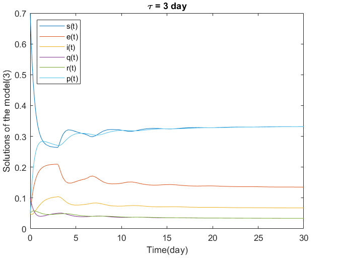
Figure 1: Dynamics of model (3) with $\tau=3$ days. Parameter values as in Table 1.

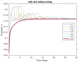
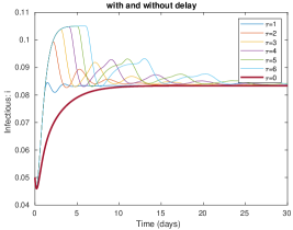
Figure 2: Dynamics of model (3) with $\tau\in[0,6]$ days. Parameter values as in Table 1.

Table 2: Parameter values used in the simulations of Section 4.2, modeling the spread of the epidemic of COVID-19 in Italy for the period of three months starting 18 October 2020.

Parameter	Value	Units	Ref
$b$	7.391‰		United:Nations
$\mu$	10.658‰		United:Nations
$\alpha$	1.1775	day-1	Cheynet
$\beta$	3.97	day-1	Cheynet
$\gamma$	0.0048	day-1	Cheynet
$\lambda$	0.0182256	day-1	Cheynet
$\delta$	0.1432		Cheynet
$t_{f}$	90	day	Assumed

In Figures 3 and 4, we present numerical solutions to the delayed model (24) in the time interval $t\in[0,90]$ days, $t=0$ representing 18 October 2020, and considering two cases:

• Case 1: $\tau=0$ days (without delay), with different percentages of susceptible individuals being vaccinated — $u=0\%$, $u=20\%$, $u=40\%$ and $u=60\%$ (Figure 3).

• Case 2: $u=20\%$ (fixed), with different delays — $\tau=0$ days, $\tau=3$ days, and $\tau=6$ days (Figure 4).

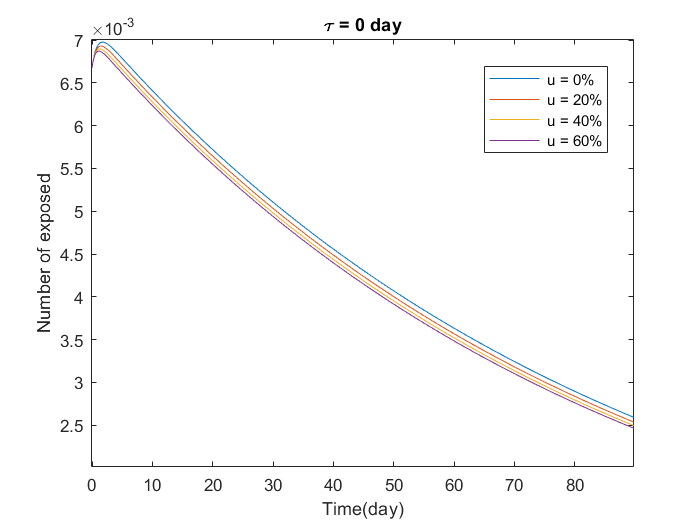
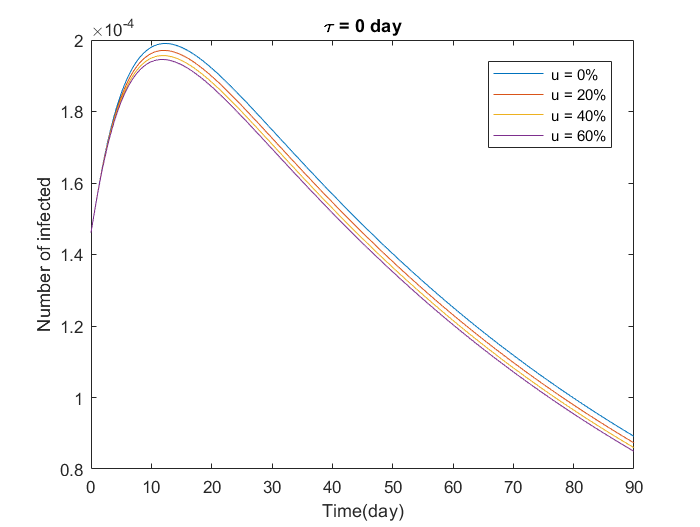
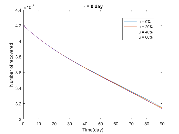
Figure 3: Predictions for Italy from the delayed model (24) with $\tau=0$ and $u\in\{0\%,20\%,40\%,60\%\}$, between 18 October 2020, and 19 January 2021.

Considering the parameter values from Table 2, and $u=0$, $u=20\%$, $u=40\%$, $u=60\%$, we have the following values for the basic reproduction number $\tilde{R}_{0}$ of Section 3: $\tilde{R}_{0}=0.0647$, $\tilde{R}_{0}=0.0554$, $\tilde{R}_{0}=0.0484$, and $\tilde{R}_{0}=0.043$, respectively. From Theorem 3.3, the disease free equilibrium $\Sigma_{1}$ of system (24) is locally asymptotically stable for the time delay $\tau=0$. From Theorem 3.3, the endemic equilibrium point $\Sigma_{V}^{+}$ of system (24) is unstable for the time delay $\tau=0$.

In conclusion, there is an inverse proportional relationship between the fraction $u$ of susceptible individuals that are vaccinated and the number of exposed, infected, and recovered individuals: the greater the fraction of susceptible individuals that are vaccinated, the smaller the number of exposed, infected, and recovered individuals would be, and vice versa (see Figure 3). Moreover, there is a directly proportional relationship between the transfer time delay $\tau$ from the class of susceptible individuals to the class of infected individuals and the number of exposed, infected, and recovered individuals: the greater the time delay, the greater the number of exposed, infected, and recovered individuals would be, and vice versa (see Figure 4).

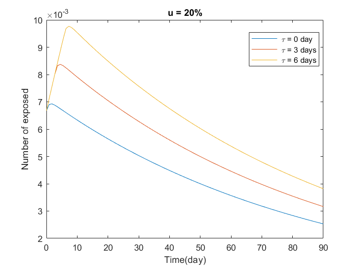
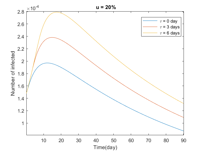
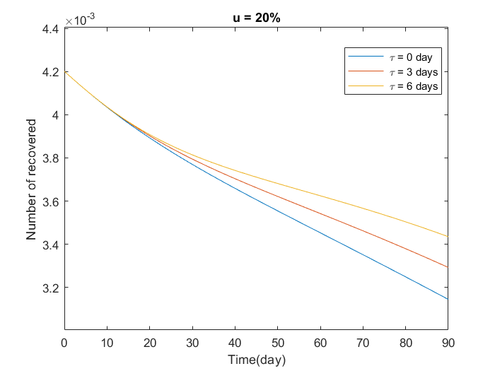
Figure 4: Predictions for Italy from the delayed model (24) with $u=20\%$ and $\tau\in\{0,3,6\}$ days, between 18 October 2020, and 19 January 2021.

Conceptualization, M.A.Z., C.J.S. and D.F.M.T.; methodology, M.A.Z., C.J.S. and D.F.M.T.; software, M.A.Z.; validation, M.A.Z., C.J.S. and D.F.M.T.; formal analysis, M.A.Z., C.J.S. and D.F.M.T.; investigation, M.A.Z., C.J.S. and D.F.M.T.; writing—original draft preparation, M.A.Z., C.J.S. and D.F.M.T.; writing—review and editing, M.A.Z., C.J.S. and D.F.M.T.; visualization, M.A.Z.; supervision, C.J.S. and D.F.M.T. All authors have read and agreed to the published version of the manuscript.

This research was funded by FCT (Fundação para a Ciência e a Tecnologia), grant number UIDB/04106/2020 (CIDMA). C.J.S. was also supported by FCT via the FCT Researcher Program CEEC Individual 2018 with reference CEECIND/00564/2018.

Not applicable.

Not applicable.

Publicly available datasets were analyzed in this study. These data can be found here: https://raw.githubusercontent.com/pcm-dpc/COVID-19/master/dati-regioni/dpc-covid19-ita-regioni.csv (accessed on 14 August 2021).

- (1) Porta, M. A Dictionary of Epidemiology; Oxford University Press: Oxford, UK, 2014. https://doi.org/10.1093/acref/9780195314496.001.0001.
- (2) WHO, World Health Organization, Available online: {http://www.emro.who.int/pandemic-epidemic-diseases/outbreaks/index.html} (accessed on 29 December 2021).
- (3) WHO, World Health Organization. Available online: {https://www.who.int/health-topics/hiv-aids} (accessed on 29 December 2021).
- (4) WHO, World Health Organization. Available online: {https://www.who.int/health-topics/tuberculosis} (accessed on 29 December 2021).
- (5) Lai, C.-C.; Shih, T.P.; Ko, W.C.; Tang, H.J.; Hsueh, P.R. Severe acute respiratory syndrome coronavirus 2 (SARS-CoV-2) and coronavirus disease-2019 (COVID-19): The epidemic and the challenges. Int. J. Antimicrob. Agents 2020, 55, 105924. https://doi.org/10.1016/j.ijantimicag.2020.105924.
- (6) Wang, L.; Wang, Y.; Ye, D.; Liu, Q. Review of the 2019 novel coronavirus (SARS-CoV-2) based on current evidence. Int. J. Antimicrob. Agents 2020, 55, 105948. https://doi.org/10.1016/j.ijantimicag.2020.105948; Erratum in: Int. J. Antimicrob. Agents 2020, 56, 106137. https://doi.org/10.1016/j.ijantimicag.2020.106137.
- (7) WHO, World Health Organization, WHO Director-General’s Opening Remarks at the Media Briefing on COVID-19. 11 March 2020. Available online: {https://www.who.int/director-general/speeches/detail/who-director-general-s-opening-remarks-at-the-media-briefing-on-covid-19---11-march-2020} (accessed on 29 December 2021).
- (8) Cappi, R.; Casini, L.; Tosi, D.; Roccetti, M. Questioning the seasonality of SARS-COV-2: A Fourier spectral analysis. BMJ Open 2022, 12, e061602. https://doi.org/10.1136/bmjopen-2022-061602.
- (9) Davis, J.T.; Chinazzi, M.; Perra, N.; Mu, K.; y Piontti, A.P.; Ajelli, M.; Dean, N.E.; Gioannini, C.; Litvinova, M.; Merler, S.; et al. Cryptic transmission of SARS-CoV-2 and the first COVID-19 wave. Nature 2021, 600, 127–132. https://doi.org/10.1038/s41586-021-04130-w.
- (10) Lemos-Paião, A.P.; Silva, C.J.; Torres, D.F.M. A new compartmental epidemiological model for COVID-19 with a case study of Portugal. Ecol. Complex. 2020, 44, 100885. https://doi.org/10.1016/j.ecocom.2020.100885. arXiv:2011.08741
- (11) Ndaïrou, F.; Area, I.; Nieto, J.J.; Silva, C.J.; Torres, D.F.M. Fractional model of COVID-19 applied to Galicia, Spain and Portugal. Chaos Solitons Fractals 2021, 144, 110652. https://doi.org/10.1016/j.chaos.2021.110652. arXiv:2101.01287
- (12) Silva, C.J.; Cruz, C.; Torres, D.F.M.; Muñuzuri, A.P.; Carballosa, A.; Area, I.; Nieto, J.J.; Fonseca-Pinto, R.; Passadouro, R.; Soares dos Santos, E.; et al. Optimal control of the COVID-19 pandemic: controlled sanitary deconfinement in Portugal. Sci. Rep. 2021, 11, 3451. https://doi.org/10.1038/s41598-021-83075-6. arXiv:2009.00660
- (13) Tang, Y.; Serdan, T.D.A.; Alecrim, A.L.; Souza, D.R.; Nacano, B.R.M.; Silva, F.L.R.; Silva, E.B.; Poma, S.O.; Gennari-Felipe, M.; Iser-Bem, P.N.; et al. A simple mathematical model for the evaluation of the long first wave of the COVID-19 pandemic in Brazil. Sci. Rep. 2021, 11, 16400. https://doi.org/10.1038/s41598-021-95815-9.
- (14) Zine, H.; Boukhouima, A.; Lotfi, E.M.; Mahrouf, M.; Torres, D.F.M.; Yousfi, N. A stochastic time-delayed model for the effectiveness of Moroccan COVID-19 deconfinement strategy. Math. Model. Nat. Phenom. 2020, 15, 50. https://doi.org/10.1051/mmnp/2020040. arXiv:2010.16265
- (15) Hernandez-Vargas, E.A.; Giordano, G.; Sontag, E.; Geoffrey, Chase, J.; Chang, H.; Astolfi, A. Second special section on systems and control research efforts against COVID-19 and future pandemics. Annu. Rev. Control 2021, 51, 424–425. https://doi.org/10.1016/j.arcontrol.2021.04.005.
- (16) Agarwal, P.; Nieto, J.J.; Ruzhansky, M.; Torres, D.F.M. Analysis of Infectious Disease Problems (COVID-19) and Their Global Impact, Infosys Science Foundation Series in Mathematical Sciences; Springer: Singapore, 2021. https://doi.org/10.1007/978-981-16-2450-6.
- (17) Arino, J. Describing, modelling and forecasting the spatial and temporal spread of COVID-19: A short review. In Mathematics of Public Health; Fields Institute Communications; Springer: Cham, Switzerland, 2022; Volume 85, pp. 25–51. https://doi.org/10.1007/978-3-030-85053-1_2.
- (18) Wang, L.; Zhang, Q.; Liu, J. On the dynamical model for COVID-19 with vaccination and time-delay effects: a model analysis supported by Yangzhou epidemic in 2021. Appl. Math. Lett. 2022, 125, 107783. https://doi.org/10.1016/j.aml.2021.107783.
- (19) Arino, J.; van den Driessche, P. Time delays in epidemic models, modeling and numerical considerations. Delay Differ. Equ. Appl. 2006, 13, 539–578. https://doi.org/10.1007/1-4020-3647-7_13.
- (20) Silva, C.J.; Maurer, H. Optimal control of HIV treatment and immunotherapy combination with state and control delays. Optim. Control Appl. Meth. 2020, 41, 537–554. https://doi.org/10.1002/oca.2558.
- (21) Silva, C.J.; Maurer, H.; Torres, D.F.M. Optimal control of a tuberculosis model with state and control delays. Math. Biosci. Eng. 2017, 14, 321–337. https://doi.org/10.3934/mbe.2017021. arXiv:1606.08721
- (22) Tipsri, S.; Chinviriyasit, W. The effect of time delay on the dynamics of an SEIR model with nonlinear incidence. Chaos Solitons Fractals 2015, 75, 153–172. https://doi.org/10.1016/j.chaos.2015.02.017.
- (23) Fine, P.E. The interval between successive cases of an infectious disease. Am. J. Epidemiol. 2003, 158, 1039–1047. https://doi.org/10.1093/aje/kwg251.
- (24) He, X.; Lau, E.H.Y.; Wu, P.; Deng, X.; Wang, J.; Hao, X.; Lau, Y.C.; Wong, J.Y.; Guan, Y.; Tan, X.; et al. Temporal dynamics in viral shedding and transmissibility of COVID-19. Nat. Med. 2020, 26, 672–675. https://doi.org/10.1038/s41591-020-0869-5.
- (25) Xin, H.; Li, Y.; Wu, P.; Li, Z.; Lau, E.H.Y.; Qin, Y.; Wang, L.; Cowling, B.J.; Tsang, T.K.; Li, Z. Estimating the latent period of coronavirus disease 2019 (COVID-19). Clin. Infect. Dis. 2022, 74, 1678–1681. https://doi.org/10.1093/cid/ciab746.
- (26) WHO, World Health Organization. Novel Coronavirus (2019-nCoV): Situation Report-7. Available online: https://apps.who.int/iris/handle/10665/330771 (accessed on 29 December 2021).
- (27) Muller, C.P. Do asymptomatic carriers of SARS-COV-2 transmit the virus? Lancet Reg. Health—Europe 2021, 4, 100082. https://doi.org/10.1016/j.lanepe.2021.100082.
- (28) Peng, L.; Yang, W.; Zhang, D.; Zhuge, C.; Hong, L. Epidemic analysis of COVID-19 in China by dynamical modeling. arXiv 2020, arXiv:2002.06563v2. https://doi.org/10.1101/2020.02.16.20023465.
- (29) Calleri, F.; Nastasi, G.; Romano, V. Continuous-time stochastic processes for the spread of COVID-19 disease simulated via a Monte Carlo approach and comparison with deterministic models. J. Math. Biol. 2021, 83, 34. https://doi.org/10.1007/s00285-021-01657-4.
- (30) Rihan, F.A.; Alsakaji, H.J.; Rajivganthi, C. Stochastic SIRC epidemic model with time-delay for COVID-19. Adv. Differ. Equ. 2020, 2020, 502. https://doi.org/10.1186/s13662-020-02964-8.
- (31) Zaitri, M.A.; Bibi, M.O.; Torres, D.F.M. Optimal control to limit the spread of COVID-19 in Italy. Kuwait J. Sci. 2021, Special Issue on COVID, 1–14. https://doi.org/10.48129/kjs.splcov.13961. arXiv:2107.11849
- (32) Lozano, M.A.; Orts, Ò.G.I.; Piñol, E.; Rebollo, M.; Polotskaya, K.; Garcia-March, M.A.; Conejero, J.A.; Escolano, F.; Oliver, N. Open Data Science to Fight COVID-19: Winning the 500k XPRIZE Pandemic Response Challenge. In Machine Learning and Knowledge Discovery in Databases. Applied Data Science Track. ECML PKDD 2021. Lecture Notes in Computer Science; Dong, Y., Kourtellis, N., Hammer, B., Lozano, J.A., Eds.; Springer: Cham, Switzerland, 2021. https://doi.org/10.1007/978-3-030-86514-6_24.
- (33) Miikkulainen, R.; Francon, O.; Meyerson, E.; Qiu, X.; Sargent, D.; Canzani, E.; Hodjat, B. From Prediction to Prescription: Evolutionary Optimization of Nonpharmaceutical Interventions in the COVID-19 Pandemic. IEEE Trans. Evol. Comput. 2021, 25, 386–401. https://doi.org/10.1109/TEVC.2021.3063217.
- (34) Giordano, G.; Blanchini, F.; Bruno, R.; Colaneri, P.; Di Filippo, A.; Di Matteo, A.; Colaneri, M. Modelling the COVID-19 epidemic and implementation of population-wide interventions in Italy. Nat. Med. 2020, 26, 855–860. https://doi.org/10.1038/s41591-020-0883-7.
- (35) Liu, Z.; Magal, P.; Seydi, O.; Webb, G. A COVID-19 epidemic model with latency period. Infect. Dis. Model. 2020, 5, 323–337. https://doi.org/10.1016/j.idm.2020.03.003.
- (36) van den Driessche, P.; Watmough, J. Reproduction numbers and sub-threshold endemic equilibria for compartmental models of disease transmission. Math. Biosci. 2002, 180, 29–48. https://doi.org/10.1016/S0025-5564(02)00108-6.
- (37) Lemos-Paião, A.P.; Silva, C.J.; Torres, D.F.M. A cholera mathematical model with vaccination and the biggest outbreak of world’s history. AIMS Math. 2018, 3, 448–463. https://doi.org/10.3934/Math.2018.4.448. arXiv:1810.05823
- (38) Rogers, J.W. Locations of roots of polynomials. SIAM Rev. 1983, 25, 327–342. https://doi.org/10.1137/1025075.
- (39) Kuang, Y. Delay Differential Equations with Applications in Population Dynamics; Mathematics in Science and Engineering, 191; Academic Press, Inc.: Boston, MA, USA, 1993.
- (40) Niculescu, S.-I. Delay Effects on Stability; Lecture Notes in Control and Information Sciences, 269; Springer: London, UK, 2001.
- (41) Shampine, L.F.; Reichelt, M.W. The MATLAB ODE suite. SIAM J. Sci. Comput. 1997, 18, 1–22. https://doi.org/10.1137/S1064827594276424.
- (42) Silva, C.J.; Cantin, G.; Cruz, C.; Fonseca-Pinto, R.; Passadouro, R.; Soares dos Santos, E.; Torres, D.F.M. Complex network model for COVID-19: human behavior, pseudo-periodic solutions and multiple epidemic waves. J. Math. Anal. Appl. 2022, 514, 125171. https://doi.org/10.1016/j.jmaa.2021.125171. arXiv:2010.02368
- (43) United Nations. The 2022 Revision of World Population Prospects. 2022. Available online: https://population.un.org/wpp/ (accessed on 29 December 2021).
- (44) Cheynet, E. Generalized SEIR Epidemic Model (Fitting and Computation); Zenodo: Transform to Open Science, NASA, Washington, D.C. 2020. https://doi.org/10.5281/ZENODO.3911854.