Efficient tensor network algorithm for layered systems
Abstract
Strongly correlated layered 2D systems are of central importance in condensed matter physics, but their numerical study is very challenging. Motivated by the enormous successes of tensor networks for 1D and 2D systems, we develop an efficient tensor network approach based on infinite projected entangled-pair states (iPEPS) for layered 2D systems. Starting from an anisotropic 3D iPEPS ansatz, we propose a contraction scheme in which the weakly-interacting layers are effectively decoupled away from the center of the layers, such that they can be efficiently contracted using 2D contraction methods while keeping the center of the layers connected in order to capture the most relevant interlayer correlations. We present benchmark data for the anisotropic 3D Heisenberg model on a cubic lattice, which shows close agreement with quantum Monte Carlo (QMC) and full 3D contraction results. Finally, we study the dimer to Néel phase transition in the Shastry-Sutherland model with interlayer coupling, a frustrated spin model which is out of reach of QMC due to the negative sign problem.
Understanding the emergent phenomena in strongly correlated systems is of central importance in modern physics. Among the most powerful tools to study these systems are tensor network (TN) methods, with the density matrix renormalization group (DMRG) [1] algorithm and its underlying variational ansatz, the matrix product state (MPS) [2, 3], being the best-known examples for (quasi) one-dimensional systems. Projected entangled-pair states (PEPS) [4, 5] (or tensor product states [6, 7, 8]) provide a natural generalization of MPS to higher dimensions. Thanks to algorithmic advances in the past years, PEPS has become a versatile state-of-the-art tool for 2D systems, not only for ground states [9, 10, 11, 12, 13, 14, 15, 16, 17, 18, 19, 20, 21, 22, 23, 24, 25, 26], but also for finite temperature calculations [27, 28, 29, 30, 31, 32, 33, 34, 35, 36, 37], excited states [38, 39, 40, 41], open systems [42, 31, 43, 44], and real-time evolution [31, 45, 46, 47, 48, 49, 50]. 3D TN algorithms are more challenging because of their higher complexity, although progress has recently been made in developing methods with a tractable computational cost [51] (see also related works on 3D classical systems [52, 53, 54, 55, 56, 57]).
A special and highly relevant class of 3D quantum systems is formed by layered 2D systems, in which the effective intralayer couplings are much stronger than the interlayer ones. Important realizations include the cuprate high-Tc superconductors [58] as well as various quasi-2D frustrated magnets such as Kagomé [59], triangular [60, 61, 62, 63, 64], Shastry-Sutherland [65, 66, 67], and honeycomb lattice compounds [68, 69, 70, 71]. While pure 2D models often already capture the relevant physics of these systems, the interlayer couplings can play an important role on the quantitative level. For example, they lead to a finite Néel transition temperature in layered square lattice Heisenberg models as opposed to the pure 2D case [72], or they may play a significant role in the competition of low-energy states in the 2D Hubbard model [12]. Thus, accurate TN approaches to study these systems would be highly desirable.
In this letter, we introduce an efficient TN algorithm for layered 2D systems, called the layered corner transfer matrix (LCTM) method, which is substantially simpler and computationally cheaper than full 3D approaches. Motivated by the layered nature of these systems, we start from an anisotropic PEPS ansatz, i.e., with a small interlayer bond dimension compared to the intralayer bond dimension , which control the accuracy of the ansatz. The main idea of the algorithm is to contract the 3D TN by (1) performing an effective decoupling of the layers away from the center of each layer, (2) contracting the individual decoupled layers using the standard 2D corner transfer matrix (CTM) method [73, 74, 10], and (3) contracting the remaining TN, formed by the contracted layers connected with a finite bond dimension in the center of each layer. A core ingredient of the approach is the effective decoupling procedure which we implement based on an iterative full-update (FU) truncation scheme [75, 76]. We present benchmark results for the anisotropic Heisenberg model on a cubic lattice, which show close agreement with a full 3D contraction and with quantum Monte Carlo (QMC) data already for small . As a more challenging example we consider a frustrated spin model, the Shastry-Sutherland model with interlayer coupling, for which QMC fails due to the negative sign problem. Finally, we highlight directions for future improvements and extensions of the LCTM approach.
Method. — We consider an infinite PEPS (iPEPS), shown in Fig. 1(a), consisting of a tensor (or more generally a unit cell of tensors) that is repeated on the infinite cubic lattice. Each tensor has 7 indices: one physical index carrying the local Hilbert space of a site, four indices with bond dimension connecting to the intraplane nearest-neighbor tensors, and two indices of dimension connecting to the tensors in the neighboring planes. The accuracy of the ansatz is systematically controlled by and , where we choose motivated by the anisotropic nature of layered 2D systems. In the limit of , the ansatz corresponds to a product state of 2D iPEPS layers, i.e., a state without entanglement between the layers (but with entanglement within the layers, controlled by ).
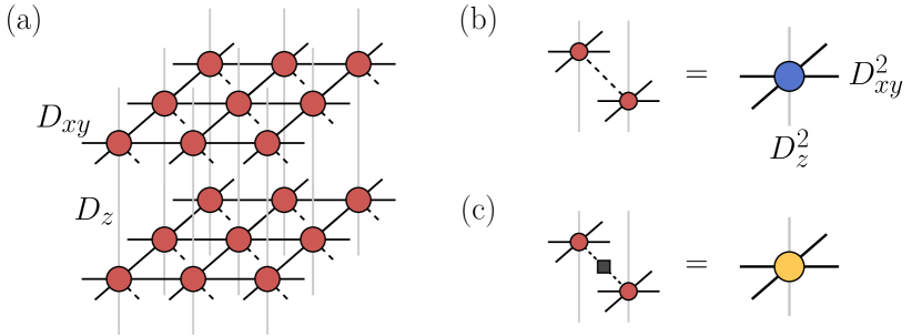
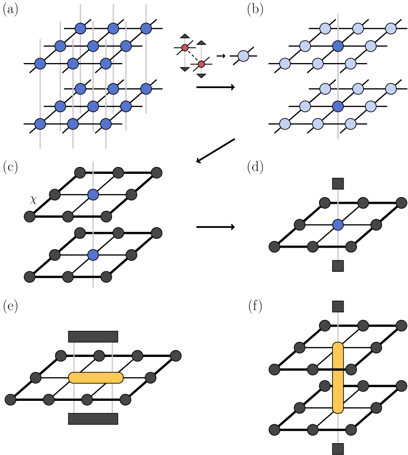
The main challenge of a 3D TN algorithm is the efficient, approximate contraction of the 3D TN, which is needed to compute, e.g., a local expectation value. Let us consider computing the norm of the wave function. The corresponding TN is depicted in Fig. 2(a), where the norm tensors (blue) represent the combined bra- and ket-tensors on each site as shown in Fig. 1(b). To compute a local expectation value, we can simply put an operator between the local tensors as shown in Fig. 1(c) and replace the norm tensor with this new tensor at the desired location.
In the simplest case, for , this network consists of independent 2D square lattice networks which can be efficiently contracted using the CTM method [73, 74, 10]. The CTM method is an iterative approach that approximates the 2D TN surrounding a central tensor by a set of environment tensors, given by four corner and four edge tensors (shown by the black disc-shaped tensors in Fig.2(c)), where the accuracy is systematically controlled by the boundary bond dimension of the environment tensors.
For the case , a full 3D contraction algorithm as in Ref. [51] could be used. This, however, is computationally expensive, and we thus follow a more efficient strategy here, exploiting the anisotropic nature of the ansatz. The main idea is to project the vertical indices of the bra- and ket-iPEPS tensors away from the center of each layer onto (see details below), while keeping the full bond dimension on the tensors in the center, see Fig. 2(b). This leads to an effective decoupling of the 2D layers away from the center, such that the standard 2D CTM approach can be used to contract them (Fig. 2(c)) while the most relevant interlayer correlations are still taken into account by the vertical connections of the tensors in the center. Since the bonds in the z-direction carry only little entanglement, the projection onto away from the center is expected to induce only a small error on a local expectation value measured in the center. After contracting each layer, the resulting TN corresponds to an infinite 1D chain in the vertical direction with bond dimension , which can be evaluated by sandwiching the central layer between the left- and right-dominant eigenvector of the corresponding transfer matrix (represented by a contracted layer), as shown in Fig. 2(d).
A core ingredient of the algorithm is the projection step from to . We use a scheme based on a full-update (FU) truncation [75, 76], a technique that is also applied in the context of imaginary time evolution algorithms to truncate a bond index in an iPEPS. It is based on a minimization of the norm distance, , which can be solved iteratively, where is the untruncated iPEPS and is the iPEPS with one bond truncated down to , see the supplemental material [77] for details. The FU does, however, require the environment tensors, which we initially do not have. We thus start from an initial approximate projection based on the simple update (SU) approach [78], which only considers local tensors for the truncation, from which the environment for the FU projection is computed. To improve the accuracy of the truncation, one can repeat the computation of the environment iteratively. In practice, for the model considered here, we find that one FU iteration is sufficient to reach convergence.
The accuracy of the LCTM method is controlled by the boundary bond dimension and by the number of connections kept in the center. Here, we focus on the simplest case, where we only keep the connections on the central tensor for the evaluation of one-site observables and interplane two-site observables (see Fig. 2(f)), which we find is sufficient in the limit of weak interlayer coupling, as we will show in our benchmark results. For intralayer two-site observables we keep two connections, as depicted in Fig. 2(e). The computational cost of these contractions are and , respectively. In the supplemental material [77] we discuss other layer decoupling approaches and we also consider a scheme with more connections, which is more accurate, but also computationally more expensive.
The LCTM contraction method can not only be used for the computation of observables, but also in combination with accurate optimization schemes (to find the optimal variational parameters in the tensors for a given Hamiltonian), e.g., in an imaginary time evolution with fast-full update (FFU) [76] or in energy minimization algorithms [79, 80, 81]. We further note that the LCTM method can be extended to arbitrary unit cell sizes in a similar way to the standard CTM in 2D [82, 10].
Results. — To benchmark the method, we consider the anisotropic 3D Heisenberg model on a cubic lattice given by the Hamiltonian
| (1) |
with the intralayer and the interlayer coupling strengths and spin operators. We use an iPEPS ansatz with two tensors, one for each sublattice, to capture the long-range antiferromagnetic order. The iPEPS is optimized with the FFU imaginary time evolution algorithm [76], starting from initial tensors obtained with simple update optimization [78]. In the CTM approach, we keep a sufficiently large boundary bond dimension , such that finite- effects are negligible [77]. To improve the computational efficiency, tensors with implemented symmetry [83, 84] are used 111We note that the SU(2) spin symmetry is broken in the ground state.. We compare our results to the ones computed with the full 3D contraction approach (SU+CTM) from Ref. [51] and with QMC results based on the directed loop algorithm from the ALPS library [86, 87] (obtained at a sufficiently low temperature of ). To extrapolate the QMC data to the thermodynamic limit, a finite size scaling analysis is performed using the scaling relations for the isotropic 3D Heisenberg model on the cubic lattice from Ref. [88] for lattices of size with up to 20 for and , and with lattices for a maximum of 12 for .
We first consider the results for the energy per site, , for in Fig. 3(a), plotted as a function of inverse bond dimension for different values of .
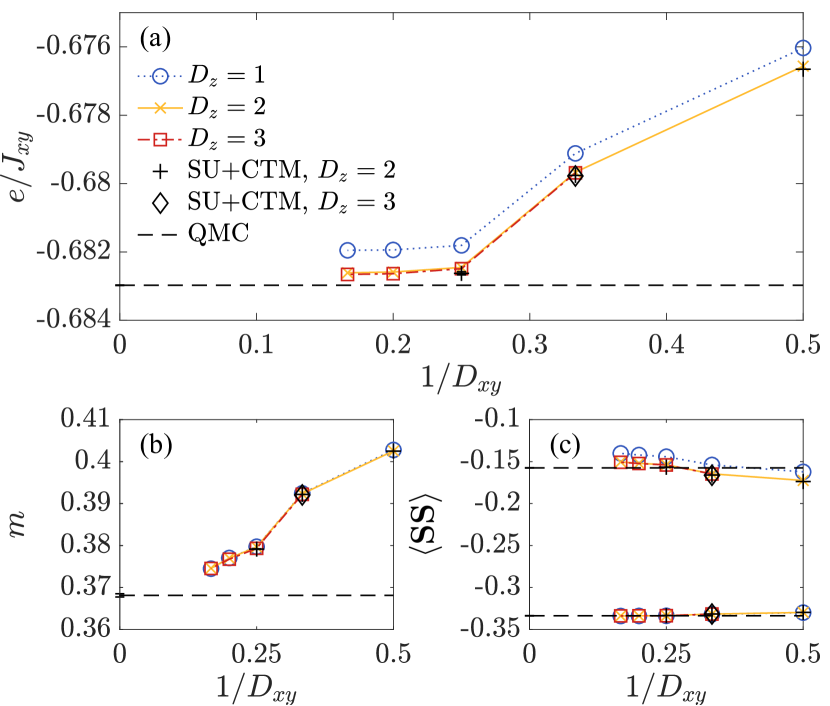
Already a product of iPEPS layers () yields a value that is remarkably close to the QMC result, with a relative error of only for . When is increased to 2, a significant improvement is found and the relative error at is reduced to , while a further increase to only yields a small enhancement. Overall, the improvement of the variational energy is clearly larger when increasing (at least up to 4) compared to the improvement when increasing , which further motivates the use of an anisotropic ansatz with . Comparing the LCTM scheme with the full 3D contraction (SU+CTM) only a small difference between the two methods is found.
Results for the local magnetic moment are shown in Fig. 3(b). Whereas systematically approaches the QMC result with increasing , the dependence on is small, suggesting that the reduction of the magnetic moment is predominantly due to the intraplane quantum fluctuations. The relative error of at and is . In Fig. 3(c) we present results for the nearest-neighbor spin-spin correlators in the intraplane and z-direction. The former is more accurately reproduced, which is a natural consequence of the fact that the latter enters with a prefactor in the optimization of the tensors. Still, we find that the QMC result is approached with increasing at large (note that increasing the two bond dimensions has an opposite effect on the change in the correlator [77]).
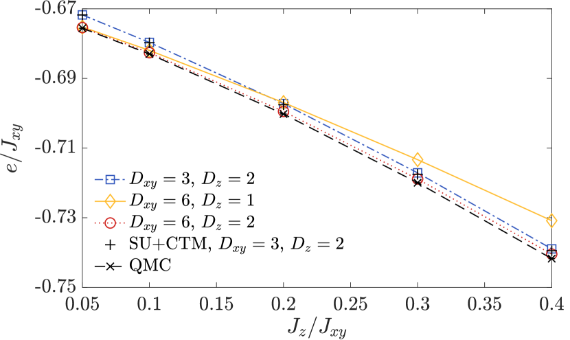
In Fig. 4 we present results for the energy per site as a function of , for selected values of and . Starting with the data for and we find that the deviation with respect to the SU+CTM result slightly increases with increasing , although the deviation remains small even at a relatively large value of . For a small ratio , a product of iPEPS layers () for already provides an energy close to the QMC result, with only a small improvement when increasing to 2. In contrast, for the energy gain is large when increasing , which is a natural consequence of the stronger entanglement between the layers for larger interlayer coupling.
We next consider a more challenging problem, the Shastry-Sutherland model [89] (SSM) - a frustrated spin model relevant for SrCu2(BO3)2 [67] for which QMC suffers from the negative sign problem [90]. It is described by square lattice layers of coupled dimers with Hamiltonian
| (2) |
with and the intra- and interdimer couplings, spin operators, and with an additional interlayer coupling to the model as in Ref. [91] (see supplemental material [77] for additional details).
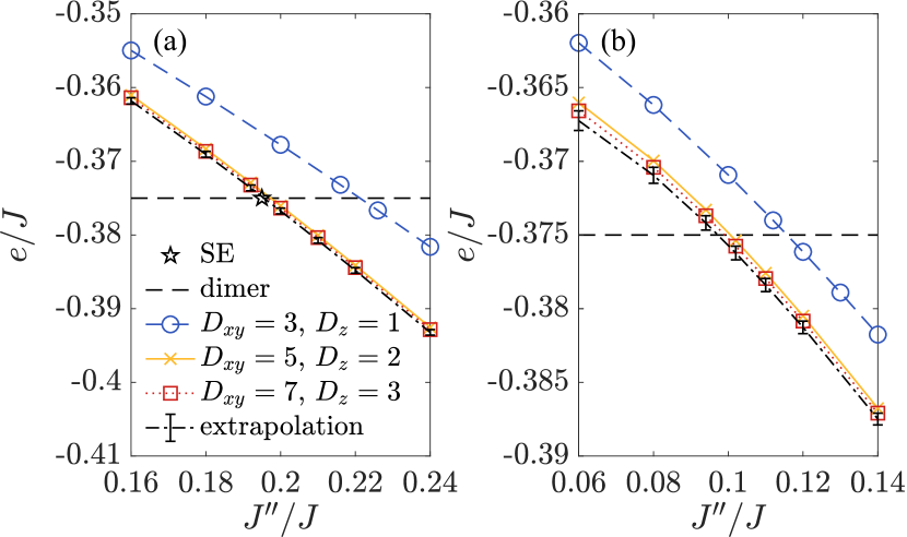
We consider the dimer to antiferromagnetic phase transition for fixed while varying and compare it to fourth-order series expansion (SE) results [91]. The location of the phase transition is determined from the intersection of the exact energy of the dimer state ( per site) with the energy of the antiferromagnetic state. For , shown in Fig. 5(a), we find a close agreement with the SE result at large bond dimensions and also based on an extrapolation in inverse bond dimension [77]. For larger values (within the dimer phase) no estimate from SE exists due to convergence problems [91]. With iPEPS, in contrast, we can accurately determine the transition, as shown in Fig. 5(b) for .
Conclusions. — We have introduced the LCTM method which is an efficient approach to study layered 2D systems with a weak interlayer coupling. The main idea is to perform a decoupling of the 3D network using the FU truncation onto away from the center of each plane, while keeping the full bond dimension in the center, such that the resulting network can be efficiently contracted with the standard CTM method in each layer. Our benchmark results for the anisotropic Heisenberg model demonstrate that the method yields values in close agreement with a full 3D contraction (SU+CTM), at a substantially lower computational cost. The results are close to QMC results even for a small interlayer bond dimension . Although the accuracy decreases when is increased, errors remain relatively small up to . Our results for the SSM demonstrate that LCTM also enables the accurate study of problems which are out of reach of QMC due to the negative sign problem.
There are several promising ways to further improve the LCTM method. First, the accuracy of the FU projection onto could be improved by making use of disentanglers between the layers [92, 93]. Second, the accuracy of the contraction can be increased by including more bonds in the center [77], although at a higher computational cost. Instead of keeping open legs with total bond dimension in between the layers, the total dimension could be effectively reduced by introducing appropriate projectors between the layers. Third, instead of a complete decoupling away from the center, a small vertical bond dimension could be kept in the CTM environment tensors in order to capture the most relevant interlayer entanglement away from the center. And finally, the contraction scheme may also be combined with an energy minimization based on automatic differentiation [81] which is expected to provide more accurate tensors than the FFU optimization used here.
We believe our approach provides a powerful and practical tool for future studies of challenging layered 2D systems, especially models that are out of reach of QMC. Finally, we note that the LCTM method can be straightforwardly extended to fermionic systems and finite temperature calculations, e.g., by adapting ideas from Refs. [94, 95, 96, 97] and Refs. [30, 31], respectively.
Acknowledgements.
This project has received funding from the European Research Council (ERC) under the European Union’s Horizon 2020 research and innovation programme (grant agreement Nos. 677061 and 101001604). This work is part of the D-ITP consortium, a program of the Netherlands Organization for Scientific Research (NWO) that is funded by the Dutch Ministry of Education, Culture, and Science (OCW).References
- White [1992] S. R. White, Phys. Rev. Lett. 69, 2863 (1992).
- Fannes et al. [1992] M. Fannes, B. Nachtergaele, and R. F. Werner, Commun. Math. Phys. 144, 443 (1992).
- Östlund and Rommer [1995] S. Östlund and S. Rommer, Phys. Rev. Lett. 75, 3537 (1995).
- Verstraete and Cirac [2004] F. Verstraete and J. I. Cirac, arXiv:cond-mat/0407066 (2004).
- Murg et al. [2007] V. Murg, F. Verstraete, and J. I. Cirac, Phys. Rev. A 75, 033605 (2007).
- Hieida et al. [1999] Y. Hieida, K. Okunishi, and Y. Akutsu, New J. Phys. 1, 7.1 (1999).
- Maeshima et al. [2001] N. Maeshima, Y. Hieida, Y. Akutsu, T. Nishino, and K. Okunishi, Phys. Rev. E 64, 016705 (2001).
- Nishio et al. [2004] Y. Nishio, N. Maeshima, A. Gendiar, and T. Nishino, arXiv:cond-mat/0401115 (2004).
- Corboz and Mila [2014] P. Corboz and F. Mila, Phys. Rev. Lett. 112, 147203 (2014).
- Corboz et al. [2014] P. Corboz, T. M. Rice, and M. Troyer, Phys. Rev. Lett. 113, 046402 (2014).
- Liao et al. [2017] H. J. Liao, Z. Y. Xie, J. Chen, Z. Y. Liu, H. D. Xie, R. Z. Huang, B. Normand, and T. Xiang, Phys. Rev. Lett. 118, 137202 (2017).
- Zheng et al. [2017] B.-X. Zheng, C.-M. Chung, P. Corboz, G. Ehlers, M.-P. Qin, R. M. Noack, H. Shi, S. R. White, S. Zhang, and G. K.-L. Chan, Science 358, 1155 (2017).
- Niesen and Corboz [2017] I. Niesen and P. Corboz, Phys. Rev. B 95, 180404(R) (2017).
- Chen et al. [2018a] J.-Y. Chen, L. Vanderstraeten, S. Capponi, and D. Poilblanc, Phys. Rev. B 98, 184409 (2018a).
- Jahromi and Orús [2018] S. S. Jahromi and R. Orús, Phys. Rev. B 98, 155108 (2018).
- Lee and Kawashima [2018] H.-Y. Lee and N. Kawashima, Phys. Rev. B 97, 205123 (2018).
- Yamaguchi et al. [2018] H. Yamaguchi, Y. Sasaki, T. Okubo, M. Yoshida, T. Kida, M. Hagiwara, Y. Kono, S. Kittaka, T. Sakakibara, M. Takigawa, Y. Iwasaki, and Y. Hosokoshi, Phys. Rev. B 98, 094402 (2018).
- Ponsioen et al. [2019] B. Ponsioen, S. S. Chung, and P. Corboz, Phys. Rev. B 100, 195141 (2019).
- Kshetrimayum et al. [2020a] A. Kshetrimayum, C. Balz, B. Lake, and J. Eisert, Ann. Phys. (N. Y.) 421, 168292 (2020a).
- Chung and Corboz [2019] S. S. Chung and P. Corboz, Phys. Rev. B 100, 035134 (2019).
- Haghshenas et al. [2019] R. Haghshenas, S.-S. Gong, and D. N. Sheng, Phys. Rev. B 99, 174423 (2019).
- Chen et al. [2020] J.-Y. Chen, S. Capponi, A. Wietek, M. Mambrini, N. Schuch, and D. Poilblanc, Phys. Rev. Lett. 125, 017201 (2020).
- Lee et al. [2020] H.-Y. Lee, R. Kaneko, L. E. Chern, T. Okubo, Y. Yamaji, N. Kawashima, and Y. B. Kim, Nat. Commun. 11, 1639 (2020).
- Gauthé et al. [2020] O. Gauthé, S. Capponi, M. Mambrini, and D. Poilblanc, Phys. Rev. B 101, 205144 (2020).
- Hasik et al. [2021] J. Hasik, D. Poilblanc, and F. Becca, SciPost Phys. 10, 012 (2021).
- Liu et al. [2021] W.-Y. Liu, J. Hasik, S.-S. Gong, D. Poilblanc, W.-Q. Chen, and Z.-C. Gu, arXiv:2110.11138 [cond-mat.str-el] (2021).
- Czarnik et al. [2017] P. Czarnik, J. Dziarmaga, and A. M. Oleś, Phys. Rev. B 96, 014420 (2017).
- Peng et al. [2017] C. Peng, S.-J. Ran, T. Liu, X. Chen, and G. Su, Phys. Rev. B 95, 075140 (2017).
- Chen et al. [2018b] X. Chen, S.-J. Ran, T. Liu, C. Peng, Y.-Z. Huang, and G. Su, Sci. Bull. 63, 1545 (2018b).
- Kshetrimayum et al. [2019] A. Kshetrimayum, M. Rizzi, J. Eisert, and R. Orús, Phys. Rev. Lett. 122, 070502 (2019).
- Czarnik et al. [2019a] P. Czarnik, J. Dziarmaga, and P. Corboz, Phys. Rev. B 99, 035115 (2019a).
- Wietek et al. [2019] A. Wietek, P. Corboz, S. Wessel, B. Normand, F. Mila, and A. Honecker, Phys. Rev. Res. 1, 033038 (2019).
- Czarnik et al. [2019b] P. Czarnik, A. Francuz, and J. Dziarmaga, Phys. Rev. B 100, 165147 (2019b).
- Czarnik et al. [2021] P. Czarnik, M. M. Rams, P. Corboz, and J. Dziarmaga, Phys. Rev. B 103, 075113 (2021).
- Jiménez et al. [2021] J. L. Jiménez, S. P. G. Crone, E. Fogh, M. E. Zayed, R. Lortz, E. Pomjakushina, K. Conder, A. M. Läuchli, L. Weber, S. Wessel, A. Honecker, B. Normand, C. Rüegg, P. Corboz, H. M. Rønnow, and F. Mila, Nature 592, 370 (2021).
- Poilblanc et al. [2021] D. Poilblanc, M. Mambrini, and F. Alet, SciPost Phys. 10, 019 (2021).
- Gauthé and Mila [2022] O. Gauthé and F. Mila, Phys. Rev. Lett. 128, 227202 (2022).
- Vanderstraeten et al. [2019] L. Vanderstraeten, J. Haegeman, and F. Verstraete, Phys. Rev. B 99, 165121 (2019).
- Ponsioen and Corboz [2020] B. Ponsioen and P. Corboz, Phys. Rev. B 101, 195109 (2020).
- Ponsioen et al. [2022] B. Ponsioen, F. Assaad, and P. Corboz, SciPost Phys. 12, 006 (2022).
- Chi et al. [2022] R.-Z. Chi, Y. Liu, Y. Wan, H.-J. Liao, and T. Xiang, arXiv:2201.12121 [cond-mat.str-el] (2022).
- Kshetrimayum et al. [2017] A. Kshetrimayum, H. Weimer, and R. Orús, Nat. Commun. 8, 1291 (2017).
- Kilda et al. [2021] D. Kilda, A. Biella, M. Schiro, R. Fazio, and J. Keeling, SciPost Physics Core 4, 005 (2021).
- Mc Keever and Szymańska [2021] C. Mc Keever and M. H. Szymańska, Phys. Rev. X 11, 021035 (2021).
- Hubig and Cirac [2019] C. Hubig and J. I. Cirac, SciPost Phys. 6, 31 (2019).
- Hubig et al. [2020] C. Hubig, A. Bohrdt, M. Knap, F. Grusdt, and J. I. Cirac, SciPost Phys. 8, 21 (2020).
- Kshetrimayum et al. [2020b] A. Kshetrimayum, M. Goihl, and J. Eisert, Phys. Rev. B 102, 235132 (2020b).
- Kshetrimayum et al. [2021] A. Kshetrimayum, M. Goihl, D. M. Kennes, and J. Eisert, Phys. Rev. B 103, 224205 (2021).
- Schmitt et al. [2021] M. Schmitt, M. M. Rams, J. Dziarmaga, M. Heyl, and W. H. Zurek, arXiv:2106.09046 [cond-mat.str-el] (2021).
- Dziarmaga [2022] J. Dziarmaga, Phys. Rev. B 105, 054203 (2022).
- Vlaar and Corboz [2021] P. C. G. Vlaar and P. Corboz, Phys. Rev. B 103, 205137 (2021).
- Nishino and Okunishi [1998] T. Nishino and K. Okunishi, J. Phys. Soc. Jpn. 67, 3066 (1998).
- Nishino et al. [2000] T. Nishino, K. Okunushi, Y. Hieida, N. Maeshima, and Y. Akutsu, Nucl. Phys. B 575, 504 (2000).
- Nishino et al. [2001] T. Nishino, Y. Hieida, K. Okunushi, N. Maeshima, Y. Akutsu, and A. Gendiar, Prog. Theor. Phys. 105, 409 (2001).
- Xie et al. [2012] Z. Y. Xie, J. Chen, M. P. Qin, J. W. Zhu, L. P. Yang, and T. Xiang, Phys. Rev. B 86, 045139 (2012).
- Orús [2012] R. Orús, Phys. Rev. B 85, 205117 (2012).
- Vanderstraeten et al. [2018] L. Vanderstraeten, B. Vanhecke, and F. Verstraete, Phys. Rev. E 98, 042145 (2018).
- Bednorz and Müller [1986] J. G. Bednorz and K. A. Müller, Z. Phys. B 64, 189 (1986).
- Shores et al. [2005] M. P. Shores, E. A. Nytko, B. M. Bartlett, and D. G. Nocera, J. Am. Chem. Soc. 127, 13462 (2005).
- Coldea et al. [2001] R. Coldea, D. A. Tennant, A. M. Tsvelik, and Z. Tylczynski, Phys. Rev. Lett. 86, 1335 (2001).
- Shimizu et al. [2003] Y. Shimizu, K. Miyagawa, K. Kanoda, M. Maesato, and G. Saito, Phys. Rev. Lett. 91, 107001 (2003).
- Shirata et al. [2012] Y. Shirata, H. Tanaka, A. Matsuo, and K. Kindo, Phys. Rev. Lett. 108, 057205 (2012).
- Rawl et al. [2017] R. Rawl, L. Ge, H. Agrawal, Y. Kamiya, C. R. Dela Cruz, N. P. Butch, X. F. Sun, M. Lee, E. S. Choi, J. Oitmaa, C. D. Batista, M. Mourigal, H. D. Zhou, and J. Ma, Phys. Rev. B 95, 060412(R) (2017).
- Cui et al. [2018] Y. Cui, J. Dai, P. Zhou, P. S. Wang, T. R. Li, W. H. Song, J. C. Wang, L. Ma, Z. Zhang, S. Y. Li, G. M. Luke, B. Normand, T. Xiang, and W. Yu, Phys. Rev. Materials 2, 044403 (2018).
- Kageyama et al. [1999] H. Kageyama, K. Yoshimura, R. Stern, N. V. Mushnikov, K. Onizuka, M. Kato, K. Kosuge, C. P. Slichter, T. Goto, and Y. Ueda, Phys. Rev. Lett. 82, 3168 (1999).
- Miyahara and Ueda [1999] S. Miyahara and K. Ueda, Phys. Rev. Lett. 82, 3701 (1999).
- Miyahara and Ueda [2003] S. Miyahara and K. Ueda, J. Phys.: Condens. Matter 15, R327 (2003).
- Singh and Gegenwart [2010] Y. Singh and P. Gegenwart, Phys. Rev. B 82, 064412 (2010).
- Plumb et al. [2014] K. W. Plumb, J. P. Clancy, L. J. Sandilands, V. V. Shankar, Y. F. Hu, K. S. Burch, H.-Y. Kee, and Y.-J. Kim, Phys. Rev. B 90, 041112(R) (2014).
- Takagi et al. [2019] H. Takagi, T. Takayama, G. Jackeli, G. Khaliullin, and S. E. Nagler, Nat Rev Phys 1, 264 (2019).
- Wessler et al. [2020] C. Wessler, B. Roessli, K. W. Krämer, B. Delley, O. Waldmann, L. Keller, D. Cheptiakov, H. B. Braun, and M. Kenzelmann, npj Quantum Mater. 5, 85 (2020).
- Sengupta et al. [2003] P. Sengupta, A. W. Sandvik, and R. R. P. Singh, Phys. Rev. B 68, 094423 (2003).
- Nishino and Okunishi [1996] T. Nishino and K. Okunishi, J. Phys. Soc. Jpn. 65, 891 (1996).
- Orús and Vidal [2009] R. Orús and G. Vidal, Phys. Rev. B 80, 094403 (2009).
- Jordan et al. [2008] J. Jordan, R. Orús, G. Vidal, F. Verstraete, and J. I. Cirac, Phys. Rev. Lett. 101, 250602 (2008).
- Phien et al. [2015] H. N. Phien, J. A. Bengua, H. D. Tuan, P. Corboz, and R. Orús, Phys. Rev. B 92, 035142 (2015).
- [77] See Supplemental Material for more technical details and additional data.
- Jiang et al. [2008] H. C. Jiang, Z. Y. Weng, and T. Xiang, Phys. Rev. Lett. 101, 090603 (2008).
- Corboz [2016] P. Corboz, Phys. Rev. B 94, 035133 (2016).
- Vanderstraeten et al. [2016] L. Vanderstraeten, J. Haegeman, P. Corboz, and F. Verstraete, Phys. Rev. B 94, 155123 (2016).
- Liao et al. [2019] H.-J. Liao, J.-G. Liu, L. Wang, and T. Xiang, Phys. Rev. X 9, 031041 (2019).
- Corboz et al. [2011] P. Corboz, S. R. White, G. Vidal, and M. Troyer, Phys. Rev. B 84, 041108(R) (2011).
- Singh et al. [2011] S. Singh, R. N. C. Pfeifer, and G. Vidal, Phys. Rev. B 83, 115125 (2011).
- Bauer et al. [2011a] B. Bauer, P. Corboz, R. Orús, and M. Troyer, Phys. Rev. B 83, 125106 (2011a).
- Note [1] We note that the SU(2) spin symmetry is broken in the ground state.
- Albuquerque et al. [2007] A. Albuquerque, F. Alet, P. Corboz, P. Dayal, A. Feiguin, S. Fuchs, L. Gamper, E. Gull, S. Gürtler, A. Honecker, R. Igarashi, M. Körner, A. Kozhevnikov, A. Läuchli, S. Manmana, M. Matsumoto, I. McCulloch, F. Michel, R. Noack, G. Pawłowski, L. Pollet, T. Pruschke, U. Schollwöck, S. Todo, S. Trebst, M. Troyer, P. Werner, and S. Wessel, J. Magn. Magn. Mater. 310, 1187 (2007).
- Bauer et al. [2011b] B. Bauer, L. D. Carr, H. G. Evertz, A. Feiguin, J. Freire, S. Fuchs, L. Gamper, J. Gukelberger, E. Gull, S. Guertler, A. Hehn, R. Igarashi, S. V. Isakov, D. Koop, P. N. Ma, P. Mates, H. Matsuo, O. Parcollet, G. Pawłowski, J. D. Picon, L. Pollet, E. Santos, V. W. Scarola, U. Schollwöck, C. Silva, B. Surer, S. Todo, S. Trebst, M. Troyer, M. L. Wall, P. Werner, and S. Wessel, J. Stat. Mech.: Theory Exp. 2011 (05), P05001.
- Hasenfratz and Niedermayer [1993] P. Hasenfratz and F. Niedermayer, Z. Phys. B 92, 91 (1993).
- Sriram Shastry and Sutherland [1981] B. Sriram Shastry and B. Sutherland, Physica B+C 108, 1069 (1981).
- Wessel et al. [2018] S. Wessel, I. Niesen, J. Stapmanns, B. Normand, F. Mila, P. Corboz, and A. Honecker, Phys. Rev. B 98, 174432 (2018).
- Koga [2000] A. Koga, J. Phys. Soc. Jpn. 69, 3509 (2000).
- Vidal [2007] G. Vidal, Phys. Rev. Lett. 99, 220405 (2007).
- Evenbly and Vidal [2015] G. Evenbly and G. Vidal, Phys. Rev. Lett. 115, 180405 (2015).
- Kraus et al. [2010] C. V. Kraus, N. Schuch, F. Verstraete, and J. I. Cirac, Phys. Rev. A 81, 052338 (2010).
- Barthel et al. [2009] T. Barthel, C. Pineda, and J. Eisert, Phys. Rev. A 80, 042333 (2009).
- Corboz et al. [2010] P. Corboz, R. Orus, B. Bauer, and G. Vidal, Phys. Rev. B 81, 165104 (2010).
- Gu et al. [2010] Z.-C. Gu, F. Verstraete, and X.-G. Wen, arXiv:1004.2563 [cont-mat.str-el] (2010).