$E_{6}$ Models in Light of Precision $M_{W}$ Measurements

Abstract

We propose a solution to the recent $W$ mass measurement by embedding the Standard Model within $E_{6}$ models. The presence of a new $U(1)$ group shifts the $W$ boson mass at the tree level and introduces a new gauge boson $Z^{\prime}$ which has been searched for at collider experiments. In this article, we identify the parameter space that explains the new $W$ mass measurement and is consistent with current experimental $Z^{\prime}$ searches. As $U(1)$ extensions can be accommodated in supersymmetric models, we also consider the supersymmetric scenario of $E_{6}$ models, and show that a 125 GeV Higgs may be easily achieved in such settings.

I Introduction

Precision measurements have been crucial in testing physics beyond the Standard Model (SM). In recent years, tensions between theory and experiment have been building with the muon $g-2$ measurement Bennett et al. (2006); Abi et al. (2021), flavor anomalies Aaij et al. (2013, 2014, 2016, 2017); Abdesselam et al. (2021); Aaij et al. (2022), and most recently the $W$ boson mass measurement by the CDF collaboration CDF Collaboration (2022). The CDF II experiment measured the $W$ boson mass to be

$$M_{W}^{\text{CDF}}=80.4335\pm 0.0094\text{ GeV},$$ (1)

which deviates from the SM prediction Workman and Others (2022) by about $7\sigma$,

$$\delta M_{W}\equiv M_{W}^{\text{CDF}}-M_{W}^{\text{SM}}\approx 76\pm 11\text{ MeV}.$$ (2)

This measurement has increased the tension between the SM and previous Tevatron measurements Aaltonen et al. (2012); Abazov et al. (2012), but is also in tension with the previous world average by more than 2$\sigma$ Workman and Others (2022). The tension between various experiments can be from unknown systematic uncertainties, which is beyond the scope of this study.

In this article, we focus on the compelling possibility that the deviation of results between the new CDF experiment, along with previous Tevatron experiments, and the SM predictions is a hint of new physics beyond the SM Cheung et al. (2022); Lu et al. (2022); Di Luzio et al. (2022); Song et al. (2022); Sakurai et al. (2022); Cheng et al. (2022a); Bahl et al. (2022a); Heo et al. (2022); Biekötter et al. (2022); Du et al. (2022a); Han et al. (2022); Ahn et al. (2022); Fileviez Perez et al. (2022); Ghoshal et al. (2022); Kanemura and Yagyu (2022); Popov and Srivastava (2022); Arcadi and Djouadi (2022); Ghorbani and Ghorbani (2022); Lee et al. (2022); Heeck (2022); Abouabid et al. (2022); Benbrik et al. (2022); Kim et al. (2022a); Strumia (2022); de Blas et al. (2022); Yang and Zhang (2022); Yuan et al. (2022); Athron et al. (2022a); Fan et al. (2022a); Babu et al. (2022); Heckman (2022); Gu et al. (2022); Athron et al. (2022b); Asadi et al. (2022); Paul and Valli (2022); Bagnaschi et al. (2022); Lee and Yamashita (2022); Liu et al. (2022); Fan et al. (2022b); Balkin et al. (2022); Endo and Mishima (2022); Crivellin et al. (2022); Han et al. (2022); Blennow et al. (2022); Cacciapaglia and Sannino (2022); Tang et al. (2022); Zhu et al. (2022); Zheng et al. (2022); Krasnikov (2022); Arias-Aragón et al. (2022); Du et al. (2022b); Kawamura et al. (2022); Nagao et al. (2022a); Zhang and Feng (2022); Carpenter et al. (2022); Chowdhury et al. (2022); Borah et al. (2022a); Zeng et al. (2022); Du et al. (2022c); Bhaskar et al. (2022); Baek (2022); Cao et al. (2022); Borah et al. (2022b); Batra et al. (2022a); Almeida et al. (2022); Cheng et al. (2022b); Batra et al. (2022b); Benbrik et al. (2022); Cai et al. (2022); Zhou and Han (2022); Gupta (2022); Wang et al. (2022); Barman et al. (2022); Kim (2022); Dcruz and Thapa (2022); Isaacson et al. (2022); Chowdhury and Saad (2022); Kim et al. (2022b); Gao et al. (2022); Lazarides et al. (2022); Rizzo (2022); Van Loi and Van Dong (2022); Yaser Ayazi and Hosseini (2022); Chakrabarty (2022); Centelles Chuliá et al. (2022); Nagao et al. (2022b); Bahl et al. (2022b); Arora et al. (2022); Heinemeyer (2022); Benakli et al. (2022); Frandsen and Rosenlyst (2022). In particular, we focus on a possible tree-level modification to the $W$ boson mass coming from an extension the SM gauge group. The simplest extension is to include a new $U(1)$ gauge group, which we call $U(1)^{\prime}$. This results in two electrically neutral gauge bosons, $Z$ and $Z^{\prime}$, that are linear combinations of the SM $Z^{0}$ boson and the gauge boson of the new $U(1)^{\prime}$ group. Due to the interconnectedness of the electroweak sector, these additions alter the $W$ boson mass at the tree level which can explain the CDF II measurement.

There are many well-motivated theories beyond the SM that feature at least one extra $U(1)$ group Rizzo (2006); Langacker (2009), such as grand unified theories (GUT) Robinett and Rosner (1982); London and Rosner (1986); Preda et al. (2022); Bajc and Senjanović (2007), superstrings Cleaver et al. (1998); Cvetic et al. (1999); Cvetič and Langacker (1996); Blumenhagen et al. (2005), extra dimensions Masip and Pomarol (1999), little Higgs Arkani-Hamed et al. (2001, 2002); Han et al. (2003), dynamical symmetry breaking Hill and Simmons (2003, 2003), and the Stueckelberg mechanism Kors and Nath (2004a, b, 2005); Feldman et al. (2006, 2007); Cheung and Yuan (2007). Among the GUT models, the ones based on rank-6 gauge groups, known as $E_{6}$ have been extensively studied for phenomenological interests Hewett and Rizzo (1989). The $E_{6}$ models can be considered in both supersymmetric and non-supersymmetric scenarios. Extending the Minimal Supersymmetric Standard Model (MSSM) with an extra $U(1)$ group also has numerous advantages. For example, similar to the Next-to-Minimal Supersymmetric Standard Model (NMSSM), the tree-level Higgs mass in the $U(1)$-supersymmetric model (UMSSM) is increased, and a 125 GeV Higgs can be obtained without the need of large radiative corrections Barger et al. (2006). Furthermore, UMSSM scenarios embed the discrete $Z_{3}$ symmetry of the NMSSM into a continuous one, and therefore, do not suffer from the cosmological domain walls problems in the NMSSM Ellis et al. (1986).

In this article, we discuss supersymmetric $E_{6}$ models in light of the CDF II $M_{W}$ measurement. We note that although our analysis is based on $E_{6}$, it can easily be generalized to any new physics scenario, supersymmetric or not, with at least one additional $U(1)^{\prime}$ gauge group. This article is structured as follows. In Sec. II, we show the contribution to the $W$ mass from the $U(1)^{\prime}$ group. In Sec. III we review the experimental constraints, especially the direct $Z^{\prime}$ searches. These constraints are then applied to $E_{6}$ models containing the $U(1)^{\prime}$ group. In Sec. IV, we discuss the predictions of the Higgs mass within supersymmetric $E_{6}$ models. Sec. V is reserved for conclusions.

II Contribution to $M_{W}$

Models that extend the SM by an extra $U(1)$ gauge group introduce a new gauge boson $Z^{\prime}$. The Cartan subalgebra of $E_{6}$ models contains two additional $U(1)$ generators. We consider the following breakdown of $E_{6}$

$$E_{6} \rightarrow SO(10)\times U(1)_{\psi}$$

$$\rightarrow SU(5)\times U(1)_{\chi}\times U(1)_{\psi}$$

$$\rightarrow SU(3)_{c}\times SU(2)_{L}\times U(1)_{Y}\times U(1)_{\chi}\times U(1)_{\psi}.$$

The two extra $U(1)$ groups yield two additional gauge bosons, $Z_{\psi}$ and $Z_{\chi}$. Upon electroweak symmetry breaking, they mix to form two gauge bosons $Z^{\prime}$ and $Z^{\prime\prime}$, with the mixing parameterized by the $E_{6}$ mixing angle $\theta_{E_{6}}$,

$$Z^{\prime} =Z_{\chi}\cos\theta_{E_{6}}+Z_{\psi}\sin\theta_{E_{6}}$$ (3)

$$Z^{\prime\prime} =-Z_{\chi}\sin\theta_{E_{6}}+Z_{\psi}\cos\theta_{E_{6}}.$$

Often, only one of the new gauge bosons is assumed to be around the TeV scale, leading to an effective rank-5 group. In this analysis, we will only consider the contributions from the lighter state of the two. We will also allow for a kinetic mixing term, $\frac{\sin{\chi}}{2}B_{\mu}Z^{\prime\mu}$ Babu et al. (1996); Chiang et al. (2014, 2015); Araz et al. (2018); Araz (2020), which has been studied in the context of a leptophobic $Z^{\prime}$. The relevant Lagrangian terms are given in the appendix.

The presence of a new $Z^{\prime}$ boson contributes to the $W$ boson mass at the tree level. The shift in the $W$ boson mass from the SM prediction can be expressed in terms of the oblique parameters $S,T,U$ Peskin and Takeuchi (1992):

$$M_{W}^{2}=(M_{W}^{\text{SM}})^{2}\\ +\frac{\alpha c_{W}^{2}}{c_{W}^{2}-s_{W}^{2}}M_{Z}^{2}\left(-\frac{1}{2}S+c_{W}^{2}T+\frac{c_{W}^{2}-s_{W}^{2}}{4s_{W}^{2}}U\right)$$ (4)

where $s_{W}$ and $c_{W}$ are the sine and cosine of the weak mixing angle, and $M_{Z}$ is the physical mass of the SM $Z^{0}$ boson. The oblique parameters may be derived from the transformation matrix responsible for bringing $\mathcal{L}$ into a basis of fields with canonical kinetic mixing and diagonal mass matrices Holdom (1991). In the appendix we derive this matrix, and from that the oblique parameters. Here we express the oblique parameters in terms of the mixing angle $\xi$ between the new $Z^{\prime}$ boson and the SM $Z^{0}$ boson, and the kinetic mixing angle $\chi$ between the $U(1)_{Y}$ and $U(1)^{\prime}$ gauge bosons. To first order in $\xi$,

$$\begin{split}\alpha S&=4c_{W}^{2}s_{W}\xi\tan{\chi},\end{split}$$ (5)

and $U=0$. $T$ is given by the wavefunction renormalization $\Delta_{Z}$ of the $Z$ boson (found in the transformation matrix) as well as the shift in the $Z$ boson mass from its SM prediction. To first order in $\xi$, the wavefunction renormalization is

$$\Delta_{Z}=s_{W}\xi\tan\chi.$$ (6)

With $Z-$$Z^{\prime}$ mass mixing, the tree-level $Z$ boson mass $M_{Z}$ is shifted from its SM value $m_{Z}$ as

$$m_{Z}^{2}=M_{Z}^{2}+[M_{Z^{\prime}}^{2}-M_{Z}^{2}]\sin^{2}{\xi}$$ (7)

which is an identical relation between the $Z-$$Z^{\prime}$ mass matrix and its diagonalized form. For small $Z-$$Z^{\prime}$ mixing angles of $\xi^{2}\ll M_{Z}^{2}/M_{Z^{\prime}}^{2}$, Eq. (7) is approximately

$$M_{Z}^{2}\approx m_{Z}^{2}\left[1-\xi^{2}\left(\frac{M_{Z^{\prime}}^{2}}{M_{Z}^{2}}-1\right)\right].$$ (8)

These changes to the properties of the $Z$ boson are combined to form the $T$ parameter:

$$\begin{split}\alpha T&=2(\Delta_{Z}-\tilde{\Delta}_{Z})\\ &=2\xi s_{W}\tan{\chi}+\xi^{2}\left(\frac{M_{Z^{\prime}}^{2}}{M_{Z}^{2}}-1\right)\end{split}$$ (9)

where $\tilde{\Delta}_{Z}$ is the fractional mass shift of $Z$ from the SM, given to first order in $\xi$.

Neglecting terms of order $\delta M_{W}^{2}$, Eq. (4) now yields the following $W$ boson mass shift:

$$\delta M_{W}\approx\frac{1}{2M_{W}}\frac{c_{W}^{4}}{c_{W}^{2}-s_{W}^{2}}\xi^{2}\left(M_{Z^{\prime}}^{2}-M_{Z}^{2}\right),$$ (10)

which only depends on the $Z^{\prime}$ mass and $Z-$$Z^{\prime}$ mixing. In Fig. 1, we plot the solution to Eq. (10) in the $M_{Z^{\prime}}-\xi$ plane.

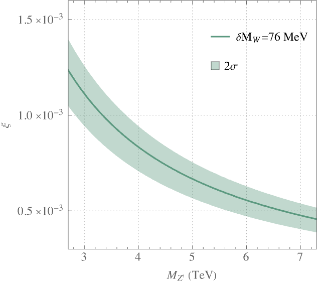
Figure 1: The solid line shows the solution to Eq. (10) for $\delta M_{W}=76$ MeV, which is the central value of the deviation of the SM from the CDF II experiment. The shaded region contains solutions for $54\,\,\text{MeV}\leq\delta M_{W}\leq 98\,\,\text{MeV}$, corresponding to a 2$\sigma$ confidence level of the CDF II measurement.

III Experimental Constraints

In this section, we will discuss various experimental constraints on a new $Z^{\prime}$ boson. The $Z^{\prime}$ may be directly produced at the Large Hadron Collider (LHC) through $p\,p\rightarrow Z^{\prime}\rightarrow l\,l$ processes, and is therefore subject to current resonant dilepton searches CMS Collaboration (2021); Aaboud et al. (2017). The results are presented as the upper limit on the product of the $Z^{\prime}$ production cross section $\sigma$ with the branching ratio of the $Z^{\prime}$ to dilepton pairs for various $Z^{\prime}$ masses, $\sigma(p\,p\rightarrow Z^{\prime})\times BR(Z^{\prime}\rightarrow l^{+}l^{-})$. Further, the results are used to constrain the Sequential Standard Model (SSM), and some rank-5 scenarios in the $E_{6}$ model. In general $E_{6}$ models, with a possible kinetic mixing term and $Z-Z^{\prime}$ mixing, the neutral current $J^{\mu}_{2}$ of the heavier mass eigenstate can be written as

$$J^{\mu}_{2}=\sum_{i}g_{Z^{\prime}}\bar{f}_{i}\gamma^{\mu}[Q_{2iL}P_{L}+Q_{2iR}P_{R}]f_{i},$$ (11)

where $g_{Z^{\prime}}$ is the coupling constant of the new gauge group. If we assume grand unification, $g_{Z^{\prime}}=0.46$ at the electroweak scale Langacker (2009). $Q_{2i(L,R)}$ are found in the appendix to be

$$\begin{split}Q_{2i(L,R)}=&\frac{g_{1}}{g_{Z^{\prime}}}c_{W}[-c_{W}\cos{\xi}\tan{\chi}]q_{i}\\ &+\frac{g_{2}}{c_{W}g_{Z^{\prime}}}[-\sin{\xi}+s_{W}\cos{\xi}\tan{\chi}]Q_{Zi(L,R)}\\ &+[\cos{\xi}/\cos{\chi}]Q^{\prime}_{i(L,R)}.\end{split}$$ (12)

The first two terms are contributions from the photon and SM $Z^{0}$ boson components in the new $Z^{\prime}$ boson due to the mixing. $g_{1}$ and $g_{2}$ are the coupling constants of the SM $U(1)_{Y}$ and $SU(2)_{L}$ gauge groups. $q_{i}$ is the electromagnetic charge of fermion $f_{i}$, and

$$Q_{Zi(L,R)}=T^{3}_{i(L,R)}-q_{i}s_{W}^{2},$$ (13)

where $T^{3}_{i(L,R)}$ is the third isospin component of fermion $f_{i}$. The last term in Eq. (12) is the contribution due to the new $U(1)^{\prime}$ gauge group and $Q^{\prime}_{i(L,R)}$ are the charges of fermions under this group.

As noted above, within $E_{6}$ models the $U(1)^{\prime}$ group is taken as an orthogonal mixture of groups $U(1)_{\chi}$ and $U(1)_{\psi}$ such that the group generators $Q^{\prime}$, $Q_{\chi}$, and $Q_{\psi}$ are related through

$$Q^{\prime}=Q_{\chi}\cos{\theta_{E_{6}}}+Q_{\psi}\sin{\theta_{E_{6}}}.$$ (14)

The charges for the fermions are listed in Table 1.

Table 2 lists canonical $E_{6}$ models which are anomaly-free without the requirement of additional massless fields. However, anomalies are present in models for all other $\theta_{E_{6}}$ values. In those cases, to cancel the anomalies, one needs to introduce the complete multiples Roepstorff (2000). Those lighter states can also contribute to $M_{W}$ through loop effects. In this article, we only focus on the tree-level effects. Those models also contain right-handed neutrinos $\nu_{R}$ for anomaly cancellation. With the right-handed neutrinos, one can generate small neutrino masses through the $Y\overline{\nu}_{R}LH_{u}+$ h.c. interaction, where $L$ is the SM leptonic doublet. However, with the $Z^{\prime}$ around the TeV scale, unless the right-handed neutrinos carry a zero $U(1)^{\prime}$ charge, as in the $N$ model, they cannot obtain the large Majorana mass needed for the conventional seesaw mechanism. In this case, small Dirac or Majorana neutrino masses are possible by invoking alternatives to the conventional seesaw mechanisim Langacker (2009).

Field	$2\sqrt{10}Q_{\chi}$	$2\sqrt{6}Q_{\psi}$
$u_{L}$	$-1$	1
$u_{R}$	1	$-1$
$d_{L}$	$-1$	1
$d_{R}$	$-3$	$-1$
$e_{L}$	3	1
$e_{R}$	1	$-1$
$\nu_{L}$	3	1
$\nu_{R}$	5	$-1$
$H_{u}$	2	$-2$
$H_{d}$	$-2$	$-2$
$S$	0	4

Table 1: $E_{6}$ charges for fermion and scalar fields following Ref. Langacker (2009).

Model	$\theta_{E_{6}}$
$\chi$	0
$\psi$	$\pi/2$
$\eta$	$-\tan^{-1}{\sqrt{5/3}}$
$I$	$\tan^{-1}{\sqrt{3/5}}$
$N$	$\tan^{-1}{\sqrt{15}}$
$S$	$\tan^{-1}{\sqrt{15}/9}$

Table 2: Canonical examples of $E_{6}$ models.

In this analysis, we recast cross-sectional bounds found by the CMS experiment by considering a ratio of cross sections in $E_{6}$ models and in the SSM. We parameterize the ratio following Ref. Barger et al. (2013),

$$\frac{\sigma(pp\rightarrow Z^{\prime}\rightarrow l^{-}l^{+})}{\sigma(pp\rightarrow Z^{\prime}_{\text{SSM}}\rightarrow l^{-}l^{+})}=\frac{pc_{u}+(1-p)c_{d}}{pc_{u,\text{SSM}}+(1-p)c_{d,\text{SSM}}}.$$ (15)

The parameter $p$ is a numerical fit depending on $M_{Z^{\prime}}/\sqrt{s}$ to account for the parton distribution function:

$$p=0.77-0.17\tan^{-1}\left(2.6-9.5\frac{M_{Z^{\prime}}}{\sqrt{s}}\right)$$ (16)

with $\sqrt{s}$ being the center-of-momentum energy. The production cross section and branching ratios are written with quantities $c_{u}$, $c_{d}$ where

$$c_{q} =\frac{M_{Z^{\prime}}g_{Z^{\prime}}^{4}}{24\pi\Gamma_{Z^{\prime}}}(Q_{2qL}^{2}+Q_{2qR}^{2})(Q_{2eL}^{2}+Q_{2eR}^{2})$$ (17)

$$c_{q,SSM} =\frac{M_{Z^{\prime}}g_{Z}^{4}}{24\pi\Gamma_{Z^{\prime}}}(Q_{ZqL}^{2}+Q_{ZqR}^{2})(Q_{ZeL}^{2}+Q_{ZeR}^{2}).$$ (18)

Here, $\Gamma_{Z^{\prime}}$ is the full width of the $Z^{\prime}$ boson found by summing partial widths for decays into massless fermion-antifermion pairs. In $E_{6}$ models,

$$\Gamma_{Z^{\prime}}=\sum_{f}g_{Z^{\prime}}^{2}\frac{M_{Z^{\prime}}}{24\pi}(Q_{2fL}^{2}+Q_{2fR}^{2}),$$ (19)

assuming negligible fermion masses. In the SSM, the couplings $g_{Z^{\prime}}$ and charges $Q_{2i(L,R)}$ are replaced by $g_{Z}\equiv g_{2}/c_{W}$ and $Q_{Zi(L,R)}$ respectively. When calculating the $Z^{\prime}$ width, we assume the new $E_{6}$ fermions are heavy enough to be ignored.

To establish a parameter space, we calculate the ratio of Eq. (15) and compare with its upper bound set by CMS searches at the LHC at $\sqrt{s}=13$ TeV, as well as CMS projections of high luminosity LHC (HL-LHC) at $\sqrt{s}=$ 14 TeV CMS Collaboration (2021, 2013). The production and decay of $Z^{\prime}$ depends on its mass $M_{Z^{\prime}}$ and the charges $Q_{2i(L,R)}$ contributing to the neutral current $J_{2}^{\mu}$. As shown in Eq. (12), $Q_{2i(L,R)}$ are determined by the $Z-$$Z^{\prime}$ mixing $\xi$, kinetic mixing $\chi$, and the $E_{6}$ mixing angle $\theta_{E_{6}}$.

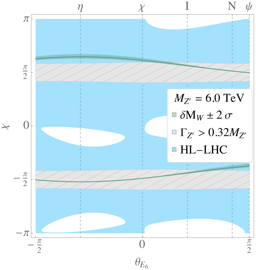
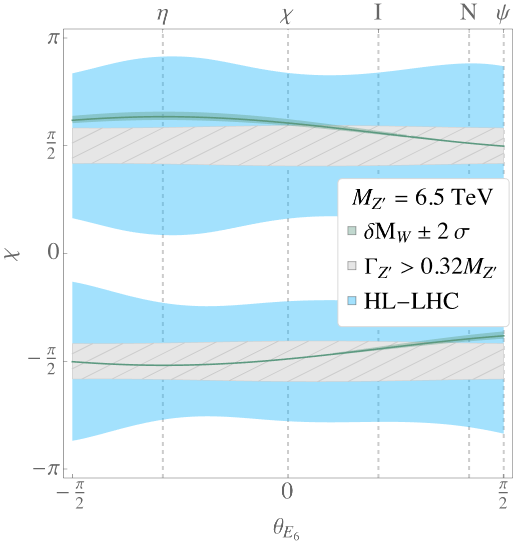
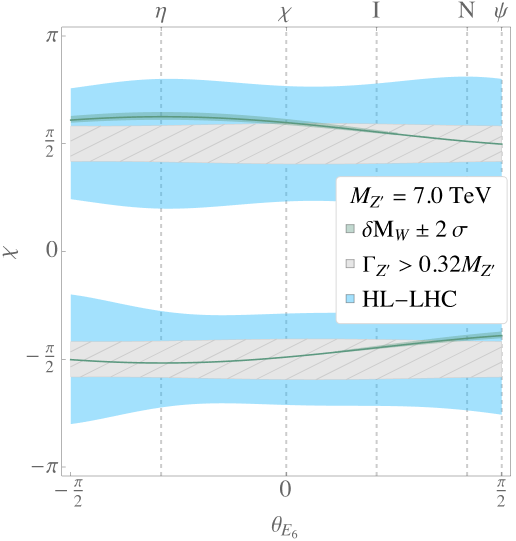
Figure 2: Parameter space probeable by HL-LHC resonant dilepton searches at 14 TeV (blue) and a wide resonance region of $\Gamma_{Z^{\prime}}/M_{Z^{\prime}}>32\%$ (gray) for $M_{Z^{\prime}}=$ 6 TeV (top), 6.5 TeV (middle), and 7 TeV (bottom). Regions consistent with the CDF II $W$ mass measurement are shown in green.

Additionally, Eq. (10) fixes $\xi$ for a given $M_{Z^{\prime}}$ to satisfy the CDF II result Eq. (2), and $\xi$ is determined by $\chi$ and $M_{Z^{\prime}}$, reducing the parameter space by two (using Eq. (36) in the appendix and $\tan\beta=10$). The $\sqrt{s}=13$ TeV search excludes $Z^{\prime}$ models that explain the CDF II result with $M_{Z^{\prime}}\leq 5.5$ TeV. At higher masses, the resulting space which may be probed by the $\sqrt{s}=14$ TeV CMS search is shown in Fig. 2 by the blue region.

There exists open parameter space around $|\chi|=\pi/2$ due to the diverging behavior of both $M_{Z^{\prime}}$ and the chiral couplings $Q_{2i(L,R)}$ in this region. As the mass and couplings increase in magnitude, so does the full width $\Gamma_{Z^{\prime}}$ of the $Z^{\prime}$ boson. This widening of $\Gamma_{Z^{\prime}}$ makes it easier for the $Z^{\prime}$ to evade direct LHC searches. We close off these regions with gray hashing in Fig. 2 where the total $Z^{\prime}$ width is more than 32% of the $Z^{\prime}$ mass following the ATLAS study in Aaboud et al. (2017). This study finds that wide resonances with $\Gamma_{Z^{\prime}}/M_{Z^{\prime}}\leq 32\%$ do not significantly affect search bounds utilizing the narrow width approximation (NWA) for $Z^{\prime}$s heavier than 4.5 TeV, and those effects become less significant as $M_{Z^{\prime}}$ increases CMS Collaboration (2021); Aaboud et al. (2017). Even so, it should be noted that our use of the NWA introduces estimated errors of $\mathcal{O}(\Gamma_{Z^{\prime}}/M_{Z^{\prime}})$ Berdine et al. (2007). Interference effects from SM gauge boson production also influence the sensitivity of collider searches. We do not consider these effects, however relative interference at the LHC can be as low as a few percent for searches that assume narrow widths Accomando et al. (2011).

For a sufficiently light $Z^{\prime}$, holes may be found in the probeable parameter space; as shown in the top panel of Fig. 2. There are two different charge suppressions responsible for the holes near the $I$ and $\eta$ models. For holes along $\theta_{E_{6}}$ near the $I$ model, these regions maintain small $Z^{\prime}$ charges for up quarks which suppress $Z^{\prime}$ production from proton collisions. On the other hand, the regions near holes along the $\eta$ model maintain small $Z^{\prime}$ charges for leptons which in turn yield small production cross sections in the lepton channels. These findings are consistent with leptophobic studies within the $\eta$ model Babu et al. (1996); Chiang et al. (2014). In either case, the $pp\rightarrow Z^{\prime}\rightarrow l^{-}l^{+}$ production inside these holes is small enough to evade the cross-sectional upper bounds found by CMS.

In addition to direct searches, a $Z^{\prime}$ gives rise to various corrections to the properties of the $Z$ boson through $Z-Z^{\prime}$ mixing parameter $\xi$, which is tightly constrained by precision $Z$ boson measurements. As shown in Fig. 1, the $Z-Z^{\prime}$ mixing required to explain the $W$ mass measurement is well below $10^{-3}$ for $Z^{\prime}$ bosons heavier than 4 TeV. The combined fit for $Z-$pole observables put an upper bound on the $Z-Z^{\prime}$ mixing parameter around $3\times 10^{-3}$ Babu et al. (1998); Erler and Langacker (2000); Ferroglia et al. (2007); Algueró et al. (2022). We have checked that the kinetic mixing introduced here did not lead to modifications beyond the current precision. For instance, a 6 TeV $Z^{\prime}$ that explains the current $W$ mass measurement in the $\eta$ model has a deviation in the leptonic decay width of the $Z$ boson of 0.0029%, which is within experimental uncertainties Workman and Others (2022).

IV Higgs Mass

In SUSY models, the mass $m_{h}$ of the Higgs boson is precisely predicted by a few relevant parameters, and can be calculated through fixed-order calculations, effective field theory (EFT) calculations, and a hybrid calculation. Dominant three-loop contributions to $m_{h}$ are known in the MSSM. (For $m_{h}$ calculation in SUSY models, see Slavich et al. (2021) and references therein.) At the tree-level, the Higgs mass has an upper bound of $M_{Z}\cos 2\beta$ in the MSSM. It receives substantial radiative corrections with the dominant contributions coming from loops involving the top, and its scalar partner, the stop, along with gluon and gluino exchanges. In particular, when the SUSY scale $M_{S}$ is around 2 TeV and the stop mixing parameter is $X_{t}\simeq-\sqrt{6}M_{S}$, a 125 GeV Higgs can be achieved with $|H^{0}_{u}|/|H^{0}_{d}|\equiv\tan\beta\gtrsim 10$ where $|H^{0}_{u}|$ is the vacuum expectation value (VEV) of the electrically neutral component of the doublet Higgs field $H_{u}$. $M_{S}$ is predicted to be at least 10 TeV from $m_{h}=125$ GeV with a vanishing stop mixing parameter Slavich et al. (2021). The current theoretical uncertainties in calculating $m_{h}$ are around 2-3 GeV for the MSSM Slavich et al. (2021).

We propose extending the SM gauge group to explain the latest $M_{W}$ measurement. Expanding into SUSY scenarios, when the MSSM is extended by an extra $U(1)$ group there are additional contributions to the $D$-term Barger et al. (2006),

$$\frac{g_{Z^{\prime}}^{2}}{2}(Q^{\prime}_{H_{d}}|H_{d}^{0}|^{2}+Q^{\prime}_{H_{u}}|H_{u}^{0}|^{2}+Q^{\prime}_{s}|S|^{2})^{2},$$ (20)

in which $H_{u}$ and $H_{d}$ are the Higgs doublets from the MSSM, and $S$ is the singlet scalar field that breaks the new $U(1)^{\prime}$ symmetry. $Q^{\prime}_{H_{u}}$, $Q^{\prime}_{H_{d}}$, and $Q^{\prime}_{s}$ are their corresponding charges under the $U(1)^{\prime}$ group. We impose the charge-conserving relation $Q^{\prime}_{H_{u}}+Q^{\prime}_{H_{d}}+Q^{\prime}_{s}=0$, coming from the $\lambda SH_{u}H_{d}$ term in the superpotential. $E_{6}$ charges for the scalar fields are given in Table 1. In addition to the new $D$-term contribution, the $\lambda SH_{u}H_{d}$ term in the superpotential increases the upper bound of the Higgs mass as in the NMSSM Maniatis (2010); Ellwanger et al. (2010). Combining both contributions, the upper bound of the Higgs mass becomes Barger et al. (2006)

$$\begin{split}m_{h}^{2}=&M_{Z}^{2}\cos^{2}2\beta+\lambda^{2}v^{2}\sin^{2}2\beta\\ &+g_{Z^{\prime}}^{2}v^{2}(Q^{\prime}_{H_{d}}\cos^{2}\beta+Q^{\prime}_{H_{u}}\sin^{2}\beta)^{2}.\end{split}$$ (21)

The increased tree-level Higgs mass implies that the stop sectors are much less constrained in the MSSM case.

To account for loop effects and the effects of the running couplings, we use FlexibleSUSY for our numerical analysis. FlexibleSUSY Athron et al. (2015, 2018) is a Mathematica and C++ package for generating mass spectra of SUSY models. It includes 2-loop Renormalization Group Equations (RGEs), it calculates $m_{h}$ at the full 1-loop level, and it includes dominant corrections up to 3-loop, next to leading logarithms. The theoretical uncertainty in the UMSSM scenario calculated in FlexibleSUSY was estimated to be as large as $\pm$10 GeV Athron et al. (2017). The large uncertainty compared to the MSSM case is due to the altered RGEs in the $E_{6}$ scenarios. For the MSSM-like parameters, we adopt a benchmark point motivated by the Natural SUSY scenario Baer et al. (2022), in which $m_{0}=7.9$ TeV, $m_{1/2}=1.2$ TeV, $\tan\beta=10$, $A_{0}=-8$ TeV, $\mu_{\text{eff}}=200$ GeV, and $m_{A}=2$ TeV. With the new $U(1)^{\prime}$ gauge group, there are two more free parameters: the gauge coupling $g_{Z^{\prime}}$ which we fix to be 0.46 from grand unification, and the VEV of the singlet field $S$, $|S|=\sqrt{2}\mu_{\text{eff}}/\lambda$ . For some $\theta_{E_{6}}$, $M_{Z^{\prime}}$, and kinetic mixing $\chi$, $|S|$ is specified, and therefore $\lambda$ is specified. As seen in Fig. 2, for a given $Z^{\prime}$ mass and $\theta_{E_{6}}$, there are two solutions in the range $-\pi\leq\chi\leq\pi$ that explain the new $W$ mass measurement. We choose the solution for which $|\chi|-\pi/2$ is maximized to avoid the diverging full width of the $Z^{\prime}$ boson at $|\chi|=\pi/2$.

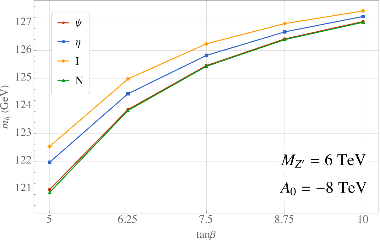
Figure 3: Masses $m_{h}$ of the lightest scalar mass eigenstate in different $E_{6}$ models for the benchmark point in Section IV ($m_{0}=7.9$ TeV, $m_{1/2}=1.2$ TeV, $A_{0}=-8$ TeV, $\mu_{\text{eff}}=200$ GeV, $m_{A}=2$ TeV) which satisfy the CDF II measurement.

Shown in Fig. 3 are predictions calculated by FlexibleSUSY for $m_{h}$, the mass of the lightest mass eigenstate within the model’s scalar sector. We fix $M_{Z^{\prime}}=6$ TeV and vary $\tan\beta$. As expected, $m_{h}$ is increased compared to the MSSM case (125 GeV for the benchmark we chose), and it is reduced as $\tan\beta$ decreases. In particular, for all $E_{6}$ scenarios we consider, $m_{h}$ is about 125 GeV for $\tan\beta\simeq$ 7 in this benchmark. Conversely, $m_{h}$ depends very weakly on $M_{Z^{\prime}}$ due to the following. The dependence of $m_{h}$ on $M_{Z^{\prime}}$ is through $\lambda=\sqrt{2}\mu_{\text{eff}}/|S|$, which is suppressed by $\sin^{2}2\beta$. Furthermore, $M_{Z^{\prime}}$ only depends on $|S|$ weakly. The dominant contribution to the $Z^{\prime}$ mass is

$$M_{Z{{}^{\prime}}}^{2}\simeq g_{Z^{\prime}}^{2}(Q_{H_{u}}^{\prime 2}v^{2}\sin^{2}\beta+Q_{H_{d}}^{\prime 2}v^{2}\cos^{2}\beta+Q_{s}^{\prime 2}|S|^{2})/\cos^{2}\chi$$ (22)

(the full result is presented in the appendix). We found that heavier a $Z^{\prime}$ requires a larger kinetic mixing $\chi$ to explain the CDF II $W$ mass measurement. This increase in $\chi$ yields a heavier $Z^{\prime}$ without requiring a large $|S|$.

Results for the $\chi$ model are not shown in Fig. 3 because $Q_{s}^{\prime}=0$ in this model. Eq. (22) shows that a heavy $Z^{\prime}$ can not be achieved with a vanishing $Q_{s}^{\prime}$ unless the gauge coupling $g_{Z}^{\prime}$ is very large. In the above numerical analysis, we do not include the kinetic mixing contribution to the $D$-term in the $m_{h}$ calculation. We have checked that it can lead to an up to $\pm$2 GeV shift in the Higgs mass at the tree-level. As discussed, when we adopt the benchmarks from the Natural SUSY scenarios, in general, the predicted $m_{h}$ is larger than 125 GeV. With the same set of parameters, we found the Higgs mass to be closer to 125 GeV with $\tan\beta\gtrsim 10$ and $A_{0}\simeq 0$ across all $E_{6}$ models discussed in this work. The possibility to accommodate a 125 GeV Higgs with small mixing in the stop sector is an encouraging feature, as the stop mixing is naturally small in minimal Anomaly mediated SUSY models Randall and Sundrum (1999); Giudice et al. (1998); Pomarol and Rattazzi (1999); Bagger et al. (2000); Jack et al. (1998); Gaillard and Nelson (2000); Binetruy et al. (2001); Dine and Seiberg (2007); de Alwis (2008); Dine and Draper (2014); Baer et al. (2018) and Gauge mediated SUSY models Dine and Fischler (1982); Dine et al. (1981); Dimopoulos and Raby (1981); Alvarez-Gaume et al. (1982); Nappi and Ovrut (1982); Eu et al. (2022); Everett et al. (2019).

	BM1 ($\eta$)	BM2 ($\eta$)	BM3 ($N$)	BM4 ($\psi$)
$\theta_{E_{6}}$ (rad)	$-0.91$	$-0.91$	$1.32$	$1.57$
$M_{Z^{\prime}}(\text{TeV})$	6	6.5	6.5	7
$A_{0}$ (TeV)	0	$-2$	$0$	$-8$
$\tan\beta$	50	8	10	7
$\chi$ (rad)	$2.03$	$1.99$	$-1.24$	$-1.23$
$m_{\tilde{t}_{1}}$ (TeV)	4.86	4.76	4.65	3.39
$m_{\tilde{\chi}_{1}^{\pm}}$ (GeV)	193	244	253	254
$m_{\tilde{\chi}_{1}^{0}}$ (GeV)	187	236	245	247
$m_{\tilde{\chi}_{2}^{0}}$ (GeV)	198	250	259	261
$m_{h}$ (GeV)	126.51	125.20	126.03	124.95
$BR(Z^{\prime}\rightarrow l^{+}l^{-})$	16.0%	16.1%	10.5%	12.5%
$\Gamma_{Z^{\prime}}/M_{Z^{\prime}}$	10.0%	12.1%	20.7%	18.1%

Table 3: Four benchmark points with predicted $M_{W}$ consistent with the CDF II measurement. For all four points, $m_{0}=7.9$ TeV, $m_{1/2}=1.2$ TeV, $\mu_{\text{eff}}=200$ GeV, and $m_{A}=2$ TeV.

In Table 3, we present four benchmark points motivated by the Natural SUSY scenario with various $Z^{\prime}$ masses. For each point, the $W$ mass is at the central value of the CDF II measurement, and the $Z^{\prime}$ mass is allowed by current CMS results. We provide in Table 3 other SUSY parameters, the Higgs mass, and the particle spectrum of the benchmark points. For all four benchmarks, the gluino mass is 3.03 TeV, which is near the projected sensitivity of the HL-LHC ATL (2014); CMS (2013). In the first three benchmarks, a Higgs mass near 125 GeV is achieved by having a small $A_{0}$. In this case, BM1 shows that a reasonable Higgs mass can be achieved with large $\tan\beta$. BM4 represents the possibility of accommodating a 125 GeV Higgs by having a small $\tan\beta$ and large mixing in the stop sector. For the electroweakino sector, as in the Natural SUSY scenarios, the lightest chargino and the two lightest neutralinos are Higgsino-like. Those electroweakinos are produced with sizable rates at the LHC and can be searched for with a soft dimuon trigger, or a hard initial state radiation jet, or through the mono-jet channel Giudice et al. (2010); Gori et al. (2013); Baer et al. (2014); Han et al. (2014, 2015); Baer et al. (2016, 2020); Arganda et al. (2021). The Higgsinos may also be accessible at lepton colliders Baer et al. (2011). Additionally, widths and leptonic branching ratios for the $Z^{\prime}$ are listed at the bottom of Table 3 with $l$ being an electron or a muon.

V Conclusion

In summary, we point out a tree-level contribution to the $W$ mass in supersymmetric $E_{6}$ models with kinetic mixing. The precision of the latest CDF II mass measurement of the $W$ boson tightly restricts $Z-$$Z^{\prime}$ mixing to be $\xi\sim O(10^{-3})$ for $Z^{\prime}$ masses in the TeV range. When combined with the direct dilepton resonance searches at the LHC, further constraints are placed on the $E_{6}$ models. For example, we have checked that for $M_{Z^{\prime}}\leq 5.5$ TeV, $\theta_{E_{6}}$ models are excluded at the $2\sigma$ level by the CDF II measurement and CMS searches at $\sqrt{s}=13$ TeV CMS Collaboration (2021). Moreover, we show how the HL-LHC run at 14 TeV is projected to further probe $E_{6}$ models for more massive $Z^{\prime}$ bosons. Additional calculations are made for the Higgs boson mass within a UMSSM. We find that a 125 GeV Higgs is possible within the reasonable parameter space allowed by experiments.

As for future directions, it will be interesting to study the associated phenomenology of the SUSY particles. With precision $W$ boson and Higgs mass measurements, the scale and mixing of the stop sector can be predicted. Motivated by the natural SUSY scenario (in which the higgsinos are light) we also expect rich phenomenology in the electroweakino sector. Thus, there is a complementarity between direct $Z^{\prime}$ searches, direct stop and electroweakino searches, and precision $M_{W}$ and $m_{h}$ measurements as they work together towards revealing new physics beyond the SM.

Appendix A

A.1 Lagrangian

There are three scalar fields in our model: two Higgs doublets from the MSSM, and a singlet scalar field that breaks the new $U(1)^{\prime}$ symmetry. Their $SU(2)_{L}\times U(1)_{Y}\times U(1)^{\prime}$ group representations are

$$H_{u} \sim(\textbf{2},1/2,Q^{\prime}_{H_{u}})$$

$$H_{d} \sim(\textbf{2},-1/2,Q^{\prime}_{H_{d}})$$

$$S \sim(\textbf{1},0,Q^{\prime}_{S}).$$

The covariant derivative is

$$D_{\mu}=\partial_{\mu}-i[g_{2}W^{a}_{\mu}T^{a}+g_{1}B_{\mu}Y+g_{Z^{\prime}}Q^{\prime}]$$

where: $W^{a}_{\mu}$, $B_{\mu}$, $Z^{\prime}_{\mu}$ are the $SU(2)_{L}$, $U(1)_{Y}$, $U(1)^{\prime}$ gauge bosons; $T^{a}$, $Y$, $Q^{\prime}$ are the group generators; $a$ runs from 1 to 3.

After the electrically neutral components of the scalar fields acquire VEVs, their kinetic terms $(D_{\mu}H)^{\dagger}D^{\mu}H$ in the Lagrangian will yield mass terms for vector fields $Z_{\mu}=c_{W}W^{3}_{\mu}-s_{W}B_{\mu}$ and $Z_{\mu}^{\prime}$ shown below. The weak mixing angle $\theta_{W}$ is defined by $s_{W}/c_{W}=\sin\theta_{W}/\cos\theta_{W}\equiv g_{1}/g_{2}$. The SM values for these parameters Workman and Others (2022) are used throughout this study.

The relevant Lagrangian terms are given by

$$\mathcal{L}\supset\mathcal{L}_{\text{mass}}+\mathcal{L}_{\text{kinetic}}+\mathcal{L}_{\text{current}},$$

$$\mathcal{L}_{\text{mass}}=-\frac{1}{2}m_{Z}^{2}Z_{\mu}Z^{\mu}-\frac{1}{2}m_{Z^{\prime}}^{2}Z^{\prime}_{\mu}Z^{\prime\mu}-\Delta^{2}Z_{\mu}Z^{\prime\mu}$$

$$\begin{split}\mathcal{L}_{\text{kinetic}}=&-\frac{1}{4}W^{3}_{\mu\nu}W^{3\mu\nu}-\frac{1}{4}B_{\mu\nu}B^{\mu\nu}-\frac{1}{4}Z^{\prime}_{\mu\nu}Z^{\prime\mu\nu}\\ &-\frac{\sin{\chi}}{2}B_{\mu\nu}Z^{\prime\mu\nu}\end{split}$$

$$\mathcal{L}_{\text{current}}=-J_{3}^{\mu}W^{3}_{\mu}-J_{Y}^{\mu}B_{\mu}-J^{\prime\mu}Z^{\prime}_{\mu}$$

where $F_{\mu\nu}$ is the field strength tensor for a gauge field $F_{\mu}$. The fermion currents are

$$J^{\mu}_{3} =g_{2}\sum_{i}\bar{f}_{i}\gamma^{\mu}[T^{3}_{iL}P_{L}+T^{3}_{iR}P_{R}]f_{i}$$ (23)

$$J^{\mu}_{Y} =g_{1}\sum_{i}\bar{f}_{i}\gamma^{\mu}[Y_{iL}P_{L}+Y_{iR}P_{R}]f_{i}$$ (24)

$$J^{\prime\mu} =g_{Z^{\prime}}\sum_{i}\bar{f}_{i}\gamma^{\mu}[Q^{\prime}_{iL}P_{L}+Q^{\prime}_{iR}P_{R}]f_{i}.$$ (25)

A group generator indexed by $iL$ ($iR$) gives the corresponding charge of the left-handed (right-handed) component of fermion field $f_{i}$. $P_{L}$ and $P_{R}$ are the left- and right-projection operators.

The terms in $\mathcal{L}$ which are absent from the SM all involve the new $Z^{\prime}_{\mu}$ gauge field. In particular, $\mathcal{L}_{\text{kinetic}}$ and $\mathcal{L}_{\text{mass}}$ contain mixing terms which must be negotiated to find the proper mass eigenstates within $\mathcal{L}_{\text{current}}$.

A.2 Kinetic Mixing

Before diagonalizing the mass matrix, we must diagonalize the kinetic mixing between the $U(1)$ and $U(1)^{\prime}$ gauge bosons. This can be done through the following $GL(3,\mathbb{R})$ transformation:

$$\begin{bmatrix}W^{3}_{\mu}\\ B_{\mu}\\ Z^{\prime}_{\mu}\end{bmatrix}=\mathbf{V}\begin{bmatrix}\hat{W}^{3}_{\mu}\\ \hat{B}_{\mu}\\ \hat{Z}^{\prime}_{\mu}\end{bmatrix},\hskip 8.5359pt\mathbf{V}\equiv\begin{bmatrix}1&0&0\\ 0&1&-\tan\chi\\ 0&0&1/\cos\chi\end{bmatrix}$$ (26)

where the hats indicate fields with canonical kinetic mixing terms. We redefine fields in an analogous way to the (neutral) electroweak sector of the SM:

$$\begin{bmatrix}A_{\mu}\\ Z_{\mu}\\ Z^{\prime}_{\mu}\end{bmatrix}=\mathbf{W}\begin{bmatrix}W^{3}_{\mu}\\ B_{\mu}\\ Z^{\prime}_{\mu}\end{bmatrix},\hskip 11.38092pt\begin{bmatrix}\hat{A}_{\mu}\\ \hat{Z}_{\mu}\\ \hat{Z}^{\prime}_{\mu}\end{bmatrix}=\mathbf{W}\begin{bmatrix}\hat{W}^{3}_{\mu}\\ \hat{B}_{\mu}\\ \hat{Z}^{\prime}_{\mu}\end{bmatrix},$$ (27)

$$\mathbf{W}\equiv\begin{bmatrix}s_{W}&c_{W}&0\\ c_{W}&-s_{W}&0\\ 0&0&1\end{bmatrix}.$$

Equation (26) may now be rewritten with the redefined fields:

$$\begin{split}\begin{bmatrix}A_{\mu}\\ Z_{\mu}\\ Z^{\prime}_{\mu}\end{bmatrix}&=\mathbf{W}\mathbf{V}\mathbf{W}^{-1}\begin{bmatrix}\hat{A}_{\mu}\\ \hat{Z}_{\mu}\\ \hat{Z}^{\prime}_{\mu}\end{bmatrix}\\ &=\begin{bmatrix}1&0&-c_{W}\tan\chi\\ 0&1&s_{W}\tan\chi\\ 0&0&1/\cos\chi\end{bmatrix}\begin{bmatrix}\hat{A}_{\mu}\\ \hat{Z}_{\mu}\\ \hat{Z}^{\prime}_{\mu}\end{bmatrix}.\end{split}$$ (28)

A.3 Mass Mixing

$\mathcal{L}_{\text{mass}}$ admits a $Z_{\mu}-Z^{\prime}_{\mu}$ mass matrix of

$$\mathbf{m}^{2}=\begin{bmatrix}m_{Z}^{2}&\Delta^{2}\\ \Delta^{2}&m_{Z^{\prime}}^{2}\end{bmatrix},$$

$$m_{Z}^{2} =\frac{1}{4}g_{Z}^{2}(|H^{0}_{u}|^{2}+|H^{0}_{d}|^{2})$$ (29)

$$m_{Z^{\prime}}^{2} =g_{Z^{\prime}}^{2}(Q_{H_{u}}^{\prime 2}|H^{0}_{u}|^{2}+Q_{H_{d}}^{\prime 2}|H^{0}_{d}|^{2}+Q_{S}^{\prime 2}|S|^{2})$$ (30)

$$\Delta^{2} =\frac{1}{2}g_{Z}g_{Z^{\prime}}(Q^{\prime}_{H_{u}}|H^{0}_{u}|^{2}-Q^{\prime}_{H_{d}}|H^{0}_{d}|^{2})$$ (31)

where $g_{Z}^{2}=g_{1}^{2}+g_{2}^{2}$ and $|H^{0}_{u}|,|H^{0}_{d}|,|S|$ are the VEVs of the electrically neutral components of the scalar fields, which we parameterize as $|H^{0}_{u}|=v\sin\beta$, $|H^{0}_{d}|=v\cos\beta$ with $v=246$ GeV. Anomaly cancellation requires $Q^{\prime}_{H_{u}}+Q^{\prime}_{H_{d}}+Q^{\prime}_{S}=0$.

In the new basis ($\hat{A}_{\mu},\hat{Z}_{\mu},\hat{Z}^{\prime}_{\mu}$) of canonical kinetic terms, the mass matrix $\mathbf{m}^{2}$ is transformed according to the ($Z_{\mu},Z^{\prime}_{\mu}$) subspace in Eq. (28). The transformation from this subspace to the ($\hat{Z}_{\mu},\hat{Z}^{\prime}_{\mu}$) subspace is given by

$$\mathbf{R}=\begin{bmatrix}1&s_{W}\tan\chi\\ 0&1/\cos\chi\end{bmatrix}$$ (32)

so that in this basis, $\mathbf{m}^{2}$ becomes

$$\begin{split}-\mathcal{L}_{\text{mass}}&=\begin{bmatrix}Z^{\mu}&Z^{\prime\mu}\end{bmatrix}\mathbf{m}^{2}\begin{bmatrix}Z_{\mu}\\ Z^{\prime}_{\mu}\end{bmatrix}\\ &=\begin{bmatrix}\hat{Z}^{\mu}&\hat{Z}^{\prime\mu}\end{bmatrix}\mathbf{R}^{T}\mathbf{m}^{2}\mathbf{R}\begin{bmatrix}\hat{Z}_{\mu}\\ \hat{Z}^{\prime}_{\mu}\end{bmatrix}\\ &\equiv\begin{bmatrix}\hat{Z}^{\mu}&\hat{Z}^{\prime\mu}\end{bmatrix}\mathbf{M}^{2}\begin{bmatrix}\hat{Z}_{\mu}\\ \hat{Z}^{\prime}_{\mu}\end{bmatrix}\end{split}$$ (33)

where the elements of $\mathbf{M}^{2}$ are

$$M^{2}_{11} =m_{Z}^{2}$$

$$M^{2}_{12} =M^{2}_{21}=\Delta^{2}/\cos\chi+m_{Z}^{2}s_{W}\tan\chi$$

$$M^{2}_{22} =m_{Z^{\prime}}^{2}/\cos^{2}\chi+m_{Z}^{2}s_{W}^{2}\tan^{2}\chi$$

$$\hskip 11.38092pt+2\Delta^{2}s_{W}\tan\chi/\cos\chi.$$

This new mass matrix $\mathbf{M}^{2}$ may be diagonalized by an orthogonal matrix

$$\mathbf{O}=\begin{bmatrix}\cos\xi&-\sin\xi\\ \sin\xi&\cos\xi\end{bmatrix}$$ (34)

and the $Z-Z^{\prime}$ mixing angle $\xi$ is given by

$$\tan{(2\xi)}=\frac{2M^{2}_{12}}{M^{2}_{11}-M^{2}_{22}}$$ (35)

or, in terms of the eigenvalues $M_{Z}^{2}$ and $M_{Z^{\prime}}^{2}$ of the matrix $\mathbf{M}^{2}$,

$$\sin{(2\xi)}=\frac{2M^{2}_{12}}{M^{2}_{Z}-M^{2}_{Z^{\prime}}},\hskip 11.38092pt\cos{(2\xi)}=\frac{M^{2}_{11}-M^{2}_{22}}{M^{2}_{Z}-M^{2}_{Z^{\prime}}}.$$ (36)

The nonzero entries of the diagonal mass matrix $\mathbf{O}^{T}\mathbf{M}^{2}\mathbf{O}$ are the tree-level squared masses of the observed $Z$ boson and a new $Z^{\prime}$,

$$M_{Z}^{2} =\frac{1}{2}\left(M^{2}_{11}+M^{2}_{22}-\sqrt{(M^{2}_{11}-M^{2}_{22})^{2}+4M^{2}_{12}}\right)$$

$$M_{Z^{\prime}}^{2} =\frac{1}{2}\left(M^{2}_{11}+M^{2}_{22}+\sqrt{(M^{2}_{11}-M^{2}_{22})^{2}+4M^{2}_{12}}\right).$$

A.4 Mass Eigenstates

After symmetry breaking, $\mathcal{L}_{\text{current}}$ becomes

$$\mathcal{L}_{\text{current}}=-J^{\mu}_{\text{em}}A_{\mu}-J^{\mu}_{Z}Z_{\mu}-J^{\prime\mu}Z^{\prime}_{\mu}$$

where these new currents are given by

$$J^{\mu}_{\text{em}} =g_{1}c_{W}\sum_{i}q_{i}\bar{f}_{i}\gamma^{\mu}f_{i}$$ (37)

$$J^{\mu}_{Z} =\frac{g_{2}}{c_{W}}\sum_{i}\bar{f}_{i}\gamma^{\mu}[Q_{ZiL}P_{L}+Q_{ZiR}P_{R}]f_{i}$$ (38)

with

$$Q_{Zi(L,R)}=T^{3}_{i(L,R)}-q_{i}s_{W}^{2}$$ (39)

where $A_{\mu}=s_{W}W^{3}_{\mu}+c_{W}B_{\mu}$ and $q_{i}\equiv T^{3}_{iL}+Y_{iL}=T^{3}_{iR}+Y_{iR}$ is the electromagnetic charge of fermion $f_{i}$ divided by the positron’s charge.

Section A.2 transforms $\mathcal{L}$ into a basis of fields with canonical kinetic mixing terms through the matrix $\mathbf{W}\mathbf{V}\mathbf{W}^{-1}$. It is then illustrated in Sec. A.3 how to transform $\mathcal{L}$ into a basis with a diagonal mass matrix using $\mathbf{O}$. Here, we combine both of these transformations, allowing us to find the mass eigenstate basis:

$$\begin{split}-\mathcal{L}_{\text{current}}&=\begin{bmatrix}J^{\mu}_{\text{em}}&J^{\mu}_{Z}&J^{\prime\mu}\end{bmatrix}\begin{bmatrix}A_{\mu}\\ Z_{\mu}\\ Z^{\prime}_{\mu}\end{bmatrix}\\ &=\begin{bmatrix}J^{\mu}_{\text{em}}&J^{\mu}_{Z}&J^{\prime\mu}\end{bmatrix}\mathbf{W}\mathbf{V}\mathbf{W}^{-1}\begin{bmatrix}1&0\\ 0&\mathbf{O}\end{bmatrix}\begin{bmatrix}\hat{A}_{\mu}\\ Z_{1\mu}\\ Z_{2\mu}\end{bmatrix}\\ &\equiv J^{\mu}_{\text{em}}\hat{A}_{\mu}+J^{\mu}_{1}Z_{1\mu}+J^{\mu}_{2}Z_{2\mu}.\end{split}$$ (40)

We identify the $Z_{1\mu}$ eigenstate with the observed $Z$ boson and the $Z_{2\mu}$ eigenstate with a hypothetical $Z^{\prime}$ boson. The currents coupled to these mass eigenstates are found through Eqs. (37), (38) as

$$J^{\mu}_{n}=\sum_{i}\bar{f}_{i}\gamma^{\mu}[Q_{niL}P_{L}+Q_{niR}P_{R}]f_{i}$$ (41)

with

$$\begin{split}Q_{1i(L,R)}=&g_{1}c_{W}[-c_{W}\sin\xi\tan\chi]q_{i}\\ &+\frac{g_{2}}{c_{W}}[\cos\xi+s_{W}\sin\xi\tan\chi]Q_{Zi(L,R)}\\ &+g_{Z^{\prime}}[\sin\xi/\cos\chi]Q^{\prime}_{i(L,R)}\end{split}$$ (42)

$$\begin{split}Q_{2i(L,R)}=&g_{1}c_{W}[-c_{W}\cos\xi\tan\chi]q_{i}\\ &+\frac{g_{2}}{c_{W}}[-\sin\xi+s_{W}\cos\xi\tan\chi]Q_{Zi(L,R)}\\ &+g_{Z^{\prime}}[\cos\xi/\cos\chi]Q^{\prime}_{i(L,R)}.\end{split}$$ (43)

The full transformation matrix of Eq. (40) is

$$\mathbf{W}\mathbf{V}\mathbf{W}^{-1}\begin{bmatrix}1&0\\ 0&\mathbf{O}\end{bmatrix}=\begin{bmatrix}1+\Delta_{A}&\Delta_{AZ}&\Delta_{AZ^{\prime}}\\ \Delta_{ZA}&1+\Delta_{Z}&\Delta_{ZZ^{\prime}}\\ \Delta_{Z^{\prime}A}&\Delta_{Z^{\prime}Z}&1+\Delta_{Z^{\prime}}\end{bmatrix}$$

$$=\begin{bmatrix}1&-c_{W}\sin\xi\tan\chi&-c_{W}\cos\xi\tan\chi\\ 0&\cos\xi+s_{W}\sin\xi\tan\chi&-\sin\xi+s_{W}\cos\xi\tan\chi\\ 0&\sin\xi/\cos\chi&\cos\xi/\cos\chi\end{bmatrix}$$

and, following Ref. Holdom (1991), the oblique parameters are given by

$$\alpha S=4c_{W}s_{W}[-(s_{W}^{2}-c_{W}^{2})\Delta_{AZ}\\ -2c_{W}s_{W}\Delta_{A}+2c_{W}s_{W}\Delta_{Z}]$$ (44)

$$\alpha U =-8s_{W}^{2}[-c_{W}s_{W}\Delta_{AZ}+s_{W}^{2}\Delta_{A}+c_{W}^{2}\Delta_{Z^{\prime}}]$$ (45)

$$\alpha T =2(\Delta_{Z}-\tilde{\Delta}_{Z})$$ (46)

where $\tilde{\Delta}_{Z}$ is the $Z$ boson’s fractional mass shift from its SM value, derived in Sec. II.

References

- Bennett et al. (2006) G. W. Bennett et al. (Muon ), Phys. Rev. D 73, 072003 (2006), arXiv:hep-ex/0602035 .
- Abi et al. (2021) B. Abi et al. (Muon Collaboration), Phys. Rev. Lett. 126, 141801 (2021).
- Aaij et al. (2013) R. Aaij et al. (LHCb), Phys. Rev. Lett. 111, 191801 (2013), arXiv:1308.1707 [hep-ex] .
- Aaij et al. (2014) R. Aaij et al. (LHCb), Phys. Rev. Lett. 113, 151601 (2014), arXiv:1406.6482 [hep-ex] .
- Aaij et al. (2016) R. Aaij et al. (LHCb), JHEP 02, 104 (2016), arXiv:1512.04442 [hep-ex] .
- Aaij et al. (2017) R. Aaij et al. (LHCb), JHEP 08, 055 (2017), arXiv:1705.05802 [hep-ex] .
- Abdesselam et al. (2021) A. Abdesselam et al. (Belle), Phys. Rev. Lett. 126, 161801 (2021), arXiv:1904.02440 [hep-ex] .
- Aaij et al. (2022) R. Aaij et al. (LHCb), Nature Phys. 18, 277 (2022), arXiv:2103.11769 [hep-ex] .
- CDF Collaboration (2022) CDF Collaboration, Science 376, 170 (2022), https://www.science.org/doi/pdf/10.1126/science.abk1781 .
- Workman and Others (2022) R. L. Workman and Others (Particle Data Group), PTEP 2022, 083C01 (2022).
- Aaltonen et al. (2012) T. Aaltonen et al. (CDF), Phys. Rev. Lett. 108, 151803 (2012), arXiv:1203.0275 [hep-ex] .
- Abazov et al. (2012) V. M. Abazov et al. (D0), Phys. Rev. Lett. 108, 151804 (2012), arXiv:1203.0293 [hep-ex] .
- Cheung et al. (2022) K. Cheung, W.-Y. Keung, and P.-Y. Tseng, “Iso-doublet Vector Leptoquark solution to the Muon , , , and -mass Anomalies,” (2022), arXiv:2204.05942 [hep-ph] .
- Lu et al. (2022) C.-T. Lu, L. Wu, Y. Wu, and B. Zhu, (2022), arXiv:2204.03796 [hep-ph] .
- Di Luzio et al. (2022) L. Di Luzio, R. Gröber, and P. Paradisi, (2022), arXiv:2204.05284 [hep-ph] .
- Song et al. (2022) H. Song, W. Su, and M. Zhang, (2022), arXiv:2204.05085 [hep-ph] .
- Sakurai et al. (2022) K. Sakurai, F. Takahashi, and W. Yin, (2022), arXiv:2204.04770 [hep-ph] .
- Cheng et al. (2022a) Y. Cheng, X.-G. He, Z.-L. Huang, and M.-W. Li, Phys. Lett. B 831, 137218 (2022a), arXiv:2204.05031 [hep-ph] .
- Bahl et al. (2022a) H. Bahl, J. Braathen, and G. Weiglein, (2022a), arXiv:2204.05269 [hep-ph] .
- Heo et al. (2022) Y. Heo, D.-W. Jung, and J. S. Lee, (2022), arXiv:2204.05728 [hep-ph] .
- Biekötter et al. (2022) T. Biekötter, S. Heinemeyer, and G. Weiglein, (2022), arXiv:2204.05975 [hep-ph] .
- Du et al. (2022a) X. K. Du, Z. Li, F. Wang, and Y. K. Zhang, (2022a), arXiv:2204.05760 [hep-ph] .
- Han et al. (2022) X.-F. Han, F. Wang, L. Wang, J. M. Yang, and Y. Zhang, (2022), arXiv:2204.06505 [hep-ph] .
- Ahn et al. (2022) Y. H. Ahn, S. K. Kang, and R. Ramos, (2022), arXiv:2204.06485 [hep-ph] .
- Fileviez Perez et al. (2022) P. Fileviez Perez, H. H. Patel, and A. D. Plascencia, (2022), arXiv:2204.07144 [hep-ph] .
- Ghoshal et al. (2022) A. Ghoshal, N. Okada, S. Okada, D. Raut, Q. Shafi, and A. Thapa, (2022), arXiv:2204.07138 [hep-ph] .
- Kanemura and Yagyu (2022) S. Kanemura and K. Yagyu, Phys. Lett. B 831, 137217 (2022), arXiv:2204.07511 [hep-ph] .
- Popov and Srivastava (2022) O. Popov and R. Srivastava, (2022), arXiv:2204.08568 [hep-ph] .
- Arcadi and Djouadi (2022) G. Arcadi and A. Djouadi, (2022), arXiv:2204.08406 [hep-ph] .
- Ghorbani and Ghorbani (2022) K. Ghorbani and P. Ghorbani, (2022), arXiv:2204.09001 [hep-ph] .
- Lee et al. (2022) S. Lee, K. Cheung, J. Kim, C.-T. Lu, and J. Song, (2022), arXiv:2204.10338 [hep-ph] .
- Heeck (2022) J. Heeck, (2022), arXiv:2204.10274 [hep-ph] .
- Abouabid et al. (2022) H. Abouabid, A. Arhrib, R. Benbrik, M. Krab, and M. Ouchemhou, (2022), arXiv:2204.12018 [hep-ph] .
- Benbrik et al. (2022) R. Benbrik, M. Boukidi, and B. Manaut, (2022), arXiv:2204.11755 [hep-ph] .
- Kim et al. (2022a) J. Kim, S. Lee, P. Sanyal, and J. Song, (2022a), arXiv:2205.01701 [hep-ph] .
- Strumia (2022) A. Strumia, (2022), arXiv:2204.04191 [hep-ph] .
- de Blas et al. (2022) J. de Blas, M. Pierini, L. Reina, and L. Silvestrini, (2022), arXiv:2204.04204 [hep-ph] .
- Yang and Zhang (2022) J. M. Yang and Y. Zhang, (2022), 10.1016/j.scib.2022.06.007, arXiv:2204.04202 [hep-ph] .
- Yuan et al. (2022) G.-W. Yuan, L. Zu, L. Feng, Y.-F. Cai, and Y.-Z. Fan, (2022), arXiv:2204.04183 [hep-ph] .
- Athron et al. (2022a) P. Athron, A. Fowlie, C.-T. Lu, L. Wu, Y. Wu, and B. Zhu, (2022a), arXiv:2204.03996 [hep-ph] .
- Fan et al. (2022a) Y.-Z. Fan, T.-P. Tang, Y.-L. S. Tsai, and L. Wu, (2022a), arXiv:2204.03693 [hep-ph] .
- Babu et al. (2022) K. S. Babu, S. Jana, and V. P. K., (2022), arXiv:2204.05303 [hep-ph] .
- Heckman (2022) J. J. Heckman, (2022), arXiv:2204.05302 [hep-ph] .
- Gu et al. (2022) J. Gu, Z. Liu, T. Ma, and J. Shu, (2022), arXiv:2204.05296 [hep-ph] .
- Athron et al. (2022b) P. Athron, M. Bach, D. H. J. Jacob, W. Kotlarski, D. Stöckinger, and A. Voigt, (2022b), arXiv:2204.05285 [hep-ph] .
- Asadi et al. (2022) P. Asadi, C. Cesarotti, K. Fraser, S. Homiller, and A. Parikh, (2022), arXiv:2204.05283 [hep-ph] .
- Paul and Valli (2022) A. Paul and M. Valli, (2022), arXiv:2204.05267 [hep-ph] .
- Bagnaschi et al. (2022) E. Bagnaschi, J. Ellis, M. Madigan, K. Mimasu, V. Sanz, and T. You, (2022), arXiv:2204.05260 [hep-ph] .
- Lee and Yamashita (2022) H. M. Lee and K. Yamashita, (2022), arXiv:2204.05024 [hep-ph] .
- Liu et al. (2022) X. Liu, S.-Y. Guo, B. Zhu, and Y. Li, (2022), arXiv:2204.04834 [hep-ph] .
- Fan et al. (2022b) J. Fan, L. Li, T. Liu, and K.-F. Lyu, (2022b), arXiv:2204.04805 [hep-ph] .
- Balkin et al. (2022) R. Balkin, E. Madge, T. Menzo, G. Perez, Y. Soreq, and J. Zupan, JHEP 05, 133 (2022), arXiv:2204.05992 [hep-ph] .
- Endo and Mishima (2022) M. Endo and S. Mishima, (2022), arXiv:2204.05965 [hep-ph] .
- Crivellin et al. (2022) A. Crivellin, M. Kirk, T. Kitahara, and F. Mescia, (2022), arXiv:2204.05962 [hep-ph] .
- Blennow et al. (2022) M. Blennow, P. Coloma, E. Fernández-Martínez, and M. González-López, (2022), arXiv:2204.04559 [hep-ph] .
- Cacciapaglia and Sannino (2022) G. Cacciapaglia and F. Sannino, Phys. Lett. B 832, 137232 (2022), arXiv:2204.04514 [hep-ph] .
- Tang et al. (2022) T.-P. Tang, M. Abdughani, L. Feng, Y.-L. S. Tsai, J. Wu, and Y.-Z. Fan, (2022), arXiv:2204.04356 [hep-ph] .
- Zhu et al. (2022) C.-R. Zhu, M.-Y. Cui, Z.-Q. Xia, Z.-H. Yu, X. Huang, Q. Yuan, and Y. Z. Fan, (2022), arXiv:2204.03767 [astro-ph.HE] .
- Zheng et al. (2022) M.-D. Zheng, F.-Z. Chen, and H.-H. Zhang, (2022), arXiv:2204.06541 [hep-ph] .
- Krasnikov (2022) N. V. Krasnikov, (2022), arXiv:2204.06327 [hep-ph] .
- Arias-Aragón et al. (2022) F. Arias-Aragón, E. Fernández-Martínez, M. González-López, and L. Merlo, (2022), arXiv:2204.04672 [hep-ph] .
- Du et al. (2022b) X. K. Du, Z. Li, F. Wang, and Y. K. Zhang, (2022b), arXiv:2204.04286 [hep-ph] .
- Kawamura et al. (2022) J. Kawamura, S. Okawa, and Y. Omura, (2022), arXiv:2204.07022 [hep-ph] .
- Nagao et al. (2022a) K. I. Nagao, T. Nomura, and H. Okada, (2022a), arXiv:2204.07411 [hep-ph] .
- Zhang and Feng (2022) K.-Y. Zhang and W.-Z. Feng, (2022), arXiv:2204.08067 [hep-ph] .
- Carpenter et al. (2022) L. M. Carpenter, T. Murphy, and M. J. Smylie, (2022), arXiv:2204.08546 [hep-ph] .
- Chowdhury et al. (2022) T. A. Chowdhury, J. Heeck, S. Saad, and A. Thapa, (2022), arXiv:2204.08390 [hep-ph] .
- Borah et al. (2022a) D. Borah, S. Mahapatra, D. Nanda, and N. Sahu, (2022a), arXiv:2204.08266 [hep-ph] .
- Zeng et al. (2022) Y.-P. Zeng, C. Cai, Y.-H. Su, and H.-H. Zhang, (2022), arXiv:2204.09487 [hep-ph] .
- Du et al. (2022c) M. Du, Z. Liu, and P. Nath, (2022c), arXiv:2204.09024 [hep-ph] .
- Bhaskar et al. (2022) A. Bhaskar, A. A. Madathil, T. Mandal, and S. Mitra, (2022), arXiv:2204.09031 [hep-ph] .
- Baek (2022) S. Baek, (2022), arXiv:2204.09585 [hep-ph] .
- Cao et al. (2022) J. Cao, L. Meng, L. Shang, S. Wang, and B. Yang, (2022), arXiv:2204.09477 [hep-ph] .
- Borah et al. (2022b) D. Borah, S. Mahapatra, and N. Sahu, Phys. Lett. B 831, 137196 (2022b), arXiv:2204.09671 [hep-ph] .
- Batra et al. (2022a) A. Batra, S. K. A., S. Mandal, and R. Srivastava, (2022a), arXiv:2204.09376 [hep-ph] .
- Almeida et al. (2022) E. d. S. Almeida, A. Alves, O. J. P. Eboli, and M. C. Gonzalez-Garcia, (2022), arXiv:2204.10130 [hep-ph] .
- Cheng et al. (2022b) Y. Cheng, X.-G. He, F. Huang, J. Sun, and Z.-P. Xing, (2022b), arXiv:2204.10156 [hep-ph] .
- Batra et al. (2022b) A. Batra, S. K. A, S. Mandal, H. Prajapati, and R. Srivastava, (2022b), arXiv:2204.11945 [hep-ph] .
- Cai et al. (2022) C. Cai, D. Qiu, Y.-L. Tang, Z.-H. Yu, and H.-H. Zhang, (2022), arXiv:2204.11570 [hep-ph] .
- Zhou and Han (2022) Q. Zhou and X.-F. Han, (2022), arXiv:2204.13027 [hep-ph] .
- Gupta (2022) R. S. Gupta, (2022), arXiv:2204.13690 [hep-ph] .
- Wang et al. (2022) J.-W. Wang, X.-J. Bi, P.-F. Yin, and Z.-H. Yu, (2022), arXiv:2205.00783 [hep-ph] .
- Barman et al. (2022) B. Barman, A. Das, and S. Sengupta, (2022), arXiv:2205.01699 [hep-ph] .
- Kim (2022) J. Kim, Phys. Lett. B 832, 137220 (2022), arXiv:2205.01437 [hep-ph] .
- Dcruz and Thapa (2022) R. Dcruz and A. Thapa, (2022), arXiv:2205.02217 [hep-ph] .
- Isaacson et al. (2022) J. Isaacson, Y. Fu, and C. P. Yuan, (2022), arXiv:2205.02788 [hep-ph] .
- Chowdhury and Saad (2022) T. A. Chowdhury and S. Saad, (2022), arXiv:2205.03917 [hep-ph] .
- Kim et al. (2022b) S.-S. Kim, H. M. Lee, A. G. Menkara, and K. Yamashita, (2022b), arXiv:2205.04016 [hep-ph] .
- Gao et al. (2022) J. Gao, D. Liu, and K. Xie, (2022), arXiv:2205.03942 [hep-ph] .
- Lazarides et al. (2022) G. Lazarides, R. Maji, R. Roshan, and Q. Shafi, (2022), arXiv:2205.04824 [hep-ph] .
- Rizzo (2022) T. G. Rizzo, (2022), arXiv:2206.09814 [hep-ph] .
- Van Loi and Van Dong (2022) D. Van Loi and P. Van Dong, (2022), arXiv:2206.10100 [hep-ph] .
- Yaser Ayazi and Hosseini (2022) S. Yaser Ayazi and M. Hosseini, (2022), arXiv:2206.11041 [hep-ph] .
- Chakrabarty (2022) N. Chakrabarty, (2022), arXiv:2206.11771 [hep-ph] .
- Centelles Chuliá et al. (2022) S. Centelles Chuliá, R. Srivastava, and S. Yadav, (2022), arXiv:2206.11903 [hep-ph] .
- Nagao et al. (2022b) K. I. Nagao, T. Nomura, and H. Okada, (2022b), arXiv:2206.15256 [hep-ph] .
- Bahl et al. (2022b) H. Bahl, W. H. Chiu, C. Gao, L.-T. Wang, and Y.-M. Zhong, (2022b), arXiv:2207.04059 [hep-ph] .
- Arora et al. (2022) S. Arora, M. Kashav, S. Verma, and B. C. Chauhan, (2022), arXiv:2207.08580 [hep-ph] .
- Heinemeyer (2022) S. Heinemeyer (2022) arXiv:2207.14809 [hep-ph] .
- Benakli et al. (2022) K. Benakli, M. Goodsell, W. Ke, and P. Slavich, (2022), arXiv:2208.05867 [hep-ph] .
- Frandsen and Rosenlyst (2022) M. T. Frandsen and M. Rosenlyst, “Electroweak precision tests of composite higgs models,” (2022).
- Rizzo (2006) T. G. Rizzo, in Theoretical Advanced Study Institute in Elementary Particle Physics: Exploring New Frontiers Using Colliders and Neutrinos (2006) pp. 537–575, arXiv:hep-ph/0610104 .
- Langacker (2009) P. Langacker, Rev. Mod. Phys. 81, 1199 (2009), arXiv:0801.1345 [hep-ph] .
- Robinett and Rosner (1982) R. W. Robinett and J. L. Rosner, Phys. Rev. D 26, 2396 (1982).
- London and Rosner (1986) D. London and J. L. Rosner, Phys. Rev. D 34, 1530 (1986).
- Preda et al. (2022) A. Preda, G. Senjanovic, and M. Zantedeschi, (2022), arXiv:2201.02785 [hep-ph] .
- Bajc and Senjanović (2007) B. Bajc and G. Senjanović, Journal of High Energy Physics 2007, 014 (2007).
- Cleaver et al. (1998) G. Cleaver, M. Cvetic, J. R. Espinosa, L. L. Everett, and P. Langacker, Phys. Rev. D 57, 2701 (1998), arXiv:hep-ph/9705391 .
- Cvetic et al. (1999) M. Cvetic, L. L. Everett, P. Langacker, and J. Wang, in Physics at Run II: Workshop on Supersymmetry / Higgs: Summary Meeting (1999) arXiv:hep-ph/9902247 .
- Cvetič and Langacker (1996) M. Cvetič and P. Langacker, Phys. Rev. D 54, 3570 (1996).
- Blumenhagen et al. (2005) R. Blumenhagen, M. Cvetic, P. Langacker, and G. Shiu, Ann. Rev. Nucl. Part. Sci. 55, 71 (2005), arXiv:hep-th/0502005 .
- Masip and Pomarol (1999) M. Masip and A. Pomarol, Phys. Rev. D 60, 096005 (1999), arXiv:hep-ph/9902467 .
- Arkani-Hamed et al. (2001) N. Arkani-Hamed, A. G. Cohen, and H. Georgi, Phys. Lett. B 513, 232 (2001), arXiv:hep-ph/0105239 .
- Arkani-Hamed et al. (2002) N. Arkani-Hamed, A. G. Cohen, E. Katz, A. E. Nelson, T. Gregoire, and J. G. Wacker, JHEP 08, 021 (2002), arXiv:hep-ph/0206020 .
- Han et al. (2003) T. Han, H. E. Logan, B. McElrath, and L.-T. Wang, Phys. Rev. D 67, 095004 (2003), arXiv:hep-ph/0301040 .
- Hill and Simmons (2003) C. T. Hill and E. H. Simmons, Phys. Rept. 381, 235 (2003), [Erratum: Phys.Rept. 390, 553–554 (2004)], arXiv:hep-ph/0203079 .
- Kors and Nath (2004a) B. Kors and P. Nath, in 10th International Symposium on Particles, Strings and Cosmology (PASCOS 04 and Pran Nath Fest) (2004) pp. 437–447, arXiv:hep-ph/0411406 .
- Kors and Nath (2004b) B. Kors and P. Nath, JHEP 12, 005 (2004b), arXiv:hep-ph/0406167 .
- Kors and Nath (2005) B. Kors and P. Nath, JHEP 07, 069 (2005), arXiv:hep-ph/0503208 .
- Feldman et al. (2006) D. Feldman, Z. Liu, and P. Nath, JHEP 11, 007 (2006), arXiv:hep-ph/0606294 .
- Feldman et al. (2007) D. Feldman, B. Kors, and P. Nath, Phys. Rev. D 75, 023503 (2007), arXiv:hep-ph/0610133 .
- Cheung and Yuan (2007) K. Cheung and T.-C. Yuan, JHEP 03, 120 (2007), arXiv:hep-ph/0701107 .
- Hewett and Rizzo (1989) J. L. Hewett and T. G. Rizzo, Phys. Rept. 183, 193 (1989).
- Barger et al. (2006) V. Barger, P. Langacker, H.-S. Lee, and G. Shaughnessy, Phys. Rev. D 73, 115010 (2006), arXiv:hep-ph/0603247 .
- Ellis et al. (1986) J. R. Ellis, K. Enqvist, D. V. Nanopoulos, K. A. Olive, M. Quiros, and F. Zwirner, Phys. Lett. B 176, 403 (1986).
- Babu et al. (1996) K. S. Babu, C. Kolda, and J. March-Russell, Phys. Rev. D 54, 4635 (1996).
- Chiang et al. (2014) C.-W. Chiang, T. Nomura, and K. Yagyu, JHEP 05, 106 (2014), arXiv:1402.5579 [hep-ph] .
- Chiang et al. (2015) C.-W. Chiang, T. Nomura, and K. Yagyu, JHEP 05, 127 (2015), arXiv:1502.00855 [hep-ph] .
- Araz et al. (2018) J. Y. Araz, G. Corcella, M. Frank, and B. Fuks, JHEP 02, 092 (2018), arXiv:1711.06302 [hep-ph] .
- Araz (2020) J. Y. Araz, in 11th International Symposium on Quantum Theory and Symmetries (2020) arXiv:2003.02177 [hep-ph] .
- Peskin and Takeuchi (1992) M. E. Peskin and T. Takeuchi, Phys. Rev. D 46, 381 (1992).
- Holdom (1991) B. Holdom, Physics Letters B 259, 329 (1991).
- CMS Collaboration (2021) CMS Collaboration, Journal of High Energy Physics 2021 (2021), 10.1007/jhep07(2021)208.
- Aaboud et al. (2017) M. Aaboud et al. (ATLAS), JHEP 10, 182 (2017), arXiv:1707.02424 [hep-ex] .
- Roepstorff (2000) G. Roepstorff, (2000), arXiv:hep-th/0005079 .
- Barger et al. (2013) V. Barger, D. Marfatia, and A. Peterson, Phys. Rev. D 87, 015026 (2013), arXiv:1206.6649 [hep-ph] .
- CMS Collaboration (2013) CMS Collaboration, (2013), arXiv:1307.7135 [hep-ex] .
- Berdine et al. (2007) D. Berdine, N. Kauer, and D. Rainwater, Phys. Rev. Lett. 99, 111601 (2007), arXiv:hep-ph/0703058 .
- Accomando et al. (2011) E. Accomando, A. Belyaev, L. Fedeli, S. F. King, and C. Shepherd-Themistocleous, Phys. Rev. D 83, 075012 (2011), arXiv:1010.6058 [hep-ph] .
- Babu et al. (1998) K. S. Babu, C. F. Kolda, and J. March-Russell, Phys. Rev. D 57, 6788 (1998), arXiv:hep-ph/9710441 .
- Erler and Langacker (2000) J. Erler and P. Langacker, Phys. Rev. Lett. 84, 212 (2000), arXiv:hep-ph/9910315 .
- Ferroglia et al. (2007) A. Ferroglia, A. Lorca, and J. J. van der Bij, Annalen Phys. 16, 563 (2007), arXiv:hep-ph/0611174 .
- Algueró et al. (2022) M. Algueró, A. Crivellin, C. A. Manzari, and J. Matias, “Unified explanation of the anomalies in semi-leptonic decays and the mass,” (2022).
- Slavich et al. (2021) P. Slavich et al., Eur. Phys. J. C 81, 450 (2021), arXiv:2012.15629 [hep-ph] .
- Maniatis (2010) M. Maniatis, Int. J. Mod. Phys. A 25, 3505 (2010), arXiv:0906.0777 [hep-ph] .
- Ellwanger et al. (2010) U. Ellwanger, C. Hugonie, and A. M. Teixeira, Phys. Rept. 496, 1 (2010), arXiv:0910.1785 [hep-ph] .
- Athron et al. (2015) P. Athron, J. hyeon Park, D. Stöckinger, and A. Voigt, Computer Physics Communications 190, 139 (2015).
- Athron et al. (2018) P. Athron, M. Bach, D. Harries, T. Kwasnitza, J. hyeon Park, D. Stöckinger, A. Voigt, and J. Ziebell, Computer Physics Communications 230, 145 (2018).
- Athron et al. (2017) P. Athron, J.-h. Park, T. Steudtner, D. Stöckinger, and A. Voigt, JHEP 01, 079 (2017), arXiv:1609.00371 [hep-ph] .
- Baer et al. (2022) H. Baer, V. Barger, and D. Martinez, Eur. Phys. J. C 82, 172 (2022), arXiv:2111.03096 [hep-ph] .
- Randall and Sundrum (1999) L. Randall and R. Sundrum, Nucl. Phys. B 557, 79 (1999), arXiv:hep-th/9810155 .
- Giudice et al. (1998) G. F. Giudice, M. A. Luty, H. Murayama, and R. Rattazzi, JHEP 12, 027 (1998), arXiv:hep-ph/9810442 .
- Pomarol and Rattazzi (1999) A. Pomarol and R. Rattazzi, JHEP 05, 013 (1999), arXiv:hep-ph/9903448 .
- Bagger et al. (2000) J. A. Bagger, T. Moroi, and E. Poppitz, JHEP 04, 009 (2000), arXiv:hep-th/9911029 .
- Jack et al. (1998) I. Jack, D. R. T. Jones, and A. Pickering, Phys. Lett. B 426, 73 (1998), arXiv:hep-ph/9712542 .
- Gaillard and Nelson (2000) M. K. Gaillard and B. D. Nelson, Nucl. Phys. B 588, 197 (2000), arXiv:hep-th/0004170 .
- Binetruy et al. (2001) P. Binetruy, M. K. Gaillard, and B. D. Nelson, Nucl. Phys. B 604, 32 (2001), arXiv:hep-ph/0011081 .
- Dine and Seiberg (2007) M. Dine and N. Seiberg, JHEP 03, 040 (2007), arXiv:hep-th/0701023 .
- de Alwis (2008) S. P. de Alwis, Phys. Rev. D 77, 105020 (2008), arXiv:0801.0578 [hep-th] .
- Dine and Draper (2014) M. Dine and P. Draper, JHEP 02, 069 (2014), arXiv:1310.2196 [hep-ph] .
- Baer et al. (2018) H. Baer, V. Barger, and D. Sengupta, Phys. Rev. D 98, 015039 (2018).
- Dine and Fischler (1982) M. Dine and W. Fischler, Phys. Lett. B 110, 227 (1982).
- Dine et al. (1981) M. Dine, W. Fischler, and M. Srednicki, Phys. Lett. B 104, 199 (1981).
- Dimopoulos and Raby (1981) S. Dimopoulos and S. Raby, Nucl. Phys. B 192, 353 (1981).
- Alvarez-Gaume et al. (1982) L. Alvarez-Gaume, M. Claudson, and M. B. Wise, Nucl. Phys. B 207, 96 (1982).
- Nappi and Ovrut (1982) C. R. Nappi and B. A. Ovrut, Phys. Lett. B 113, 175 (1982).
- Eu et al. (2022) S. T. Eu, L. L. Everett, T. Garon, and N. Leonard, Phys. Rev. D 105, 055019 (2022), arXiv:2110.05599 [hep-ph] .
- Everett et al. (2019) L. L. Everett, T. S. Garon, and A. B. Rock, Phys. Rev. D 100, 015039 (2019), arXiv:1812.10811 [hep-ph] .
- ATL (2014) Search for Supersymmetry at the high luminosity LHC with the ATLAS experiment, Tech. Rep. (CERN, Geneva, 2014).
- CMS (2013) Study of the Discovery Reach in Searches for Supersymmetry at CMS with 3000/fb, Tech. Rep. (CERN, Geneva, 2013).
- Giudice et al. (2010) G. F. Giudice, T. Han, K. Wang, and L.-T. Wang, Phys. Rev. D 81, 115011 (2010), arXiv:1004.4902 [hep-ph] .
- Gori et al. (2013) S. Gori, S. Jung, and L.-T. Wang, JHEP 10, 191 (2013), arXiv:1307.5952 [hep-ph] .
- Baer et al. (2014) H. Baer, A. Mustafayev, and X. Tata, Phys. Rev. D 90, 115007 (2014).
- Han et al. (2014) Z. Han, G. D. Kribs, A. Martin, and A. Menon, Phys. Rev. D 89, 075007 (2014), arXiv:1401.1235 [hep-ph] .
- Han et al. (2015) C. Han, D. Kim, S. Munir, and M. Park, JHEP 04, 132 (2015), arXiv:1502.03734 [hep-ph] .
- Baer et al. (2016) H. Baer, V. Barger, M. Savoy, and X. Tata, Phys. Rev. D 94, 035025 (2016), arXiv:1604.07438 [hep-ph] .
- Baer et al. (2020) H. Baer, V. Barger, S. Salam, D. Sengupta, and X. Tata, Phys. Lett. B 810, 135777 (2020), arXiv:2007.09252 [hep-ph] .
- Arganda et al. (2021) E. Arganda, A. Delgado, R. A. Morales, and M. Quirós, Phys. Rev. D 104, 055003 (2021), arXiv:2104.13827 [hep-ph] .
- Baer et al. (2011) H. Baer, V. Barger, and P. Huang, JHEP 11, 031 (2011), arXiv:1107.5581 [hep-ph] .