Signatures of cooperative emission in photon coincidence: Superradiance versus measurement-induced cooperativity

Abstract

Indistinguishable quantum emitters confined to length scales smaller than the wavelength of the light become superradiant. Compared to uncorrelated and distinguishable emitters, superradiance results in qualitative modifications of optical signals such as photon coincidences. However, recent experiments revealed that similar signatures can also be obtained in situations where emitters are too far separated to be superradiant if correlations between emitters are induced by the wave function collapse during an emission-angle-selective photon detection event. Here, we compare two sources for cooperative emission, superradiance and measurement-induced cooperativity, and analyze their impact on time-dependent optical signals. We find that an anti-dip in photon coincidences at zero time delay is a signature of inter-emitter correlations in general but does not unambiguously prove the presence of superradiance. This suggests that photon coincidences at zero time delay alone are not sufficient and time-dependent data is necessary to clearly demonstrate a superradiant enhancement of the spontaneous radiative decay rate.

I Introduction

Spontaneous photon emission is one of the most elementary processes in quantum physics[1, 2]. In many situations, it is appropriately described by the conversion of excitations of quantum emitters into photons with some fixed rate $\Gamma$ depending on the particular emitter[1]. However, a closer look reveals that even spontaneous emission can reveal interesting insights into fundamental aspects of quantum mechanics. For example, it has been realized that radiative decay not only depends on the emitters themselves but also on their photonic environment. Drexhage et al.[3] famously observed substantial changes of photon emission rates when emitters are placed close to a mirror. Nowadays, photonic structures like waveguides[4, 5], optical microcavities[6, 7], or photonic crystals[8, 9] have become key elements of solid state quantum devices relying on efficient photon extraction via the Purcell effect or on spectral filtering via resonances in the photonic environment[10, 11, 12, 13, 14].

Moreover, even the emission into free space can reveal intricate effects of cooperative emission when multiple indistinguishable quantum emitters are involved, such as in the case of superradiance[15, 16, 17]: On a semiclassical level, superradiance can be understood by the fact that the spontaneous emission rate of a single quantum emitter $\gamma$ is proportional to the modulus square of the transition dipole $\mathbf{d}$. Confining $N$ emitters to volumes smaller than the wavelength of the light, so that the light field effectively interacts with a single large dipole $\mathbf{D}=N\mathbf{d}$, hence yields a spontaneous emission rate of up to $N^{2}\gamma$ as opposed to the emission from $N$ individual emitters, each with rate $\gamma$. A more detailed quantum mechanical treatment[15, 16] reveals emission to take place via a cascade through the Dicke ladder, a set of strongly correlated states with excitations equally distributed across many emitters. The superextensive light-matter coupling is also the reason why the reverse process, superabsorption[18, 19], has been proposed for applications, e.g., in quantum batteries[20].

Even though applications typically rely on cooperative effects in the large-$N$ limit, experiments can also provide valuable insights for samples with only $N=2$ or $N=3$ emitters as these often facilitate a direct control, e. g., varying the degree of indistinguishability by tuning emitters in and out of resonance[4, 21, 22]. In the low-$N$ limit, photon coincidence measurements are particularly useful because the violation of the upper bound of zero-delay coincidences $g^{(2)}(0)\leq(N-1)/N$ for uncorrelated emitters is clear proof for inter-emitter correlations (cf. Appendix B). For example, values of $g^{(2)}(0)\approx 1$ have been used as the main piece of evidence for superradiance of semiconductor quantum dots coupled to a nanophotonic waveguide in the case of $N=2$ emitters[4]. Similarly, for $N=3$ quantum dots, values exceeding $g^{(2)}(0)>1$ have been reported[21].

Recently, the radiation pattern of light scattering at two identical trapped ions[24, 25], has added yet another dimension to the discussion of cooperative emission. There, photon coincidences $g^{(2)}(0)$ have been demonstrated to exceed or fall below the expected value of $1/2$ for two identical uncorrelated emitters, depending on the detection angle. This can be explained by a measurement-induced preparation of a correlated Dicke-like state by the first photon detection event, which shapes the radiation pattern for the subsequent emission of a second photon[26, 27]. It is noteworthy that these results are also found when the separation of the emitters exceeds the wavelength of the light, where superradiance, as discussed by Dicke[15], is not expected.

We have recently demonstrated a solid-state quantum device where two semiconductor quantum dots (QDs) can be electrically tuned into resonance[22]. This device operates in a similar regime as the experiments on trapped ions in that the emitters are spectrally indistinguishable but the spatial separation exceeds the value for which superradiance is expected. In contrast to Refs. [24, 25], we additionally investigated temporal aspects such as free radiative decay for situations corresponding to distinguishable and indistinguishable emitters, respectively, using different driving conditions like continous pumping and pulsed excitation[22]. Detecting photons in the direction perpendicular to the plane containing the QDs, we indeed found signatures in photon coincidences resembling those expected from superradiance, such as values of $g^{(2)}(0)>1/2$, but at the same time no evidence of superradiant rate enhancement was observed in the free radiative decay.

These observations raise important conceptual questions: How exactly is the physical situation in Refs. [24, 25] and [22] related to superradiance? If an anti-dip in $g^{(2)}(\tau)$ with $g^{(2)}(0)$ exceeding the limit for independent emitters is not a unique signature of superradiance, how can both situations be distinguished by measurement?

While many aspects of superradiance, measurement-induced coherence, and interference of light emitted from quantum emitters at fixed positions have been thoroughly investigated (see, e.g., Refs. [26, 28, 29]), most previous works either neglect dephasing or primarily focus on static quantities such as photon coincidences $g^{(2)}(0)$ at zero delay time only. To obtain a realistic description of cooperative emission including coherent and time-dependent driving as well as unavoidable dephasing in solid-state systems, we here rephrase the emission dynamics employing an open quantum systems framework for the density matrix of the emitter system. This allows us to treat superradiance as well as measurement-induced cooperative photon emission within a single framework, and to discuss common features as well as differences.

Before presenting our main results relating to time-dependent optical signals, we introduce our framework through a detailed pedagogical derivation, also applying it to elementary examples and recovering well-known limiting cases [15, 29, 28]. To preclude confusion, here, we stick to definitions where we use the term “cooperative emission” to refer to general situations where more than one emitter is involved in a single photon emission process, while we reserve “superradiance” exclusively for situations where cooperative emission additionally leads to an increase of the overall radiative decay rate, i.e. to enhanced radiance. In these terms, Dicke superradiance and measurement-induced cooperativity by emission-angle-selective measurement can be viewed as two different instances of cooperative emission, even though the latter does not show any superradiant rate enhancement.

Once these concepts have been clarified, we use our framework to present numerical and analytical calculations of time-dependent photon coincidences for continuously pumped emitters as well as for emitters under pulsed driving, while simultaneously properly accounting for effects of dephasing. Our results elucidate how signatures of cooperative emission manifest in experimentally relevant situations, and highlights pitfalls relating to the correct interpretation of measured data. As a key insight we find that, in the presence of dephasing, the photon coincidence trace for measurement-induced cooperativity is qualitatively remarkably similar to that of superradiant decay. This reflects the fact that both rely on the presence of correlations between emitters in general rather than being an unequivocal indicator of a superradient decay rate enhancement. Similarly, care has to be taken when interpreting time-integrated photon coincidences after pulsed driving: for single and indistinguishable emitters, time-integrated coincidences are found to have the same value as the corresponding zero-delay coincidences $g^{(2)}(0)$ for incoherently pumped emitters, but the link between these two quantities generally does not carry over to cooperatively emitting quantum emitters.

This article is structured as follows: First we (re-)derive established results for radiative decay and photon coincidences from two emitters with identical dipoles in the cases of distinguishable and superradiant emitters. We then generalise the treatment to obtain a framework in which general photon emission as well as the effects of angle-resolved detection can be discussed, which naturally leads to the observation of cooperative emission due to selective measurement. Finally, we calculate concrete optical signals such as the full delay-time dependent photon coincidences $g^{(2)}(\tau)$ in this regime under the assumption of incoherent continuous driving as well as time-integrated coincidences for a system of emitters driven by short laser pulses.

II Radiative decay of distinguishable and superradiant emitters

Throughout this article, we consider the case of two emitters located at positions $\mathbf{r}_{1}=-\mathbf{r}/2$ and $\mathbf{r}_{2}=\mathbf{r}/2$, respectively. Modelling the $i$-th emitter as a two-level system with ground and excited states $|g_{i}\rangle$ and $|e_{i}\rangle$, respectively, and introducing operators $\sigma^{+}_{i}=|e_{i}\rangle\langle g_{i}|$ and $\sigma^{-}_{i}=|g_{i}\rangle\langle e_{i}|$, the total Hamiltonian of the emitter system coupled to the light field modes is

$$H= H_{0}+H_{I},$$ (1a)

$$H_{0}= \sum_{i=1,2}\hbar\omega_{i}\sigma^{+}_{i}\sigma^{-}_{i}+\sum_{\mathbf{k},\lambda}\hbar\omega_{\mathbf{k}}a^{\dagger}_{\mathbf{k},\lambda}a_{\mathbf{k},\lambda},$$ (1b)

$$H_{I}= \sum_{\mathbf{k},\lambda}\big{(}h_{\mathbf{k},\lambda}a^{\dagger}_{\mathbf{k},\lambda}+h_{\mathbf{k},\lambda}^{\dagger}a_{\mathbf{k},\lambda}\big{)},$$ (1c)

$$h_{\mathbf{k},\lambda}= \hbar\big{(}g_{1,\mathbf{k},\lambda}\,e^{i\mathbf{k}\cdot\mathbf{r}/2}\sigma^{-}_{1}+g_{2,\mathbf{k},\lambda}\,e^{-i\mathbf{k}\cdot\mathbf{r}/2}\sigma^{-}_{2}\big{)},$$ (1d)

where $a^{\dagger}_{\mathbf{k},\lambda}$ and $a_{\mathbf{k},\lambda}$ are creation and annihilation operators of photons with wave vector $\mathbf{k}$ and polarization $\lambda$, $\hbar\omega_{\mathbf{k}}$ is the energy of the respective photon mode, and $\hbar\omega_{i}$ is the fundamental transition energy of the $i$-th emitter. Here, we assume identical light-matter coupling strengths $g_{1,\mathbf{k},\lambda}=g_{2,\mathbf{k},\lambda}=g_{\mathbf{k},\lambda}$ for both emitters and all photon modes $\mathbf{k}$, where $g_{\mathbf{k},\lambda}=(\hat{\mathbf{d}}\cdot\mathbf{e}_{\mathbf{k},\lambda})^{2}g$ with constant $g$, normalized direction of the dipole $\hat{\mathbf{d}}=\mathbf{d}/|\mathbf{d}|$, and polarization vector $\mathbf{e}_{\mathbf{k},\lambda}$. For a more convenient notation, we henceforth drop the polarization index $\lambda$ unless necessary.

If the emitters are spectrally distinguishable, i.e., there is vanishing overlap between the spectral lines at $\hbar\omega_{1}$ and $\hbar\omega_{2}$, radiative decay can be described by non-degenerate perturbation theory using Fermi’s golden rule, which predicts a decay rate

$$\gamma_{\textnormal{i}\to\textnormal{f}}= \frac{2\pi}{\hbar}\sum_{\mathbf{k}}\big{|}\langle\textnormal{f}|h_{\mathbf{k}}|\textnormal{i}\rangle\big{|}^{2}\delta(E_{\textnormal{i}}-E_{\textnormal{f}}-\hbar\omega_{\mathbf{k}}),$$ (2)

where $|\textnormal{i}\rangle$ and $|\textnormal{f}\rangle$ are the initial and final states of the decay process, which are eigenstates of the unperturbed problem $H_{0}$, and $E_{\textnormal{i}}$ and $E_{\textnormal{f}}$ are the corresponding energies. For two distinguishable emitters, the energy eigenstates are product states of the emitters in ground or excited states $|e_{1},e_{2}\rangle$, $|e_{1},g_{2}\rangle$, $|g_{1},e_{2}\rangle$, and $|g_{1},g_{2}\rangle$.

Assuming a flat photon density of states $D(E)=\sum_{\mathbf{k},\lambda}\delta(E-\hbar\omega_{\mathbf{k}})(\hat{\mathbf{d}}\cdot\mathbf{e}_{\mathbf{k},\lambda})^{2}=D$ within the range of the relevant energies, the radiative decay rates for all processes where one excitation is emitted as a photon, as depicted in Fig. 1a, are identical $\gamma=2\pi\hbar g^{2}D$.

For spectrally indistinguishable emitters with $\omega_{1}=\omega_{2}$, non-degenerate perturbation theory no longer applies and the degeneracy has to be addressed explicitly. An important special case is the superradiant regime, where the distance between emitters is much smaller than the wavelength of the light $\mathbf{k}\cdot\mathbf{r}\approx 0$. Then, the phase factors in the interaction term $h_{\mathbf{k}}$ are $e^{\pm i\mathbf{k}\cdot\mathbf{r}/2}\approx 1$ and one can replace $h_{\mathbf{k}}=h_{S}$ with

$$h_{S}= \hbar\sqrt{2}g\sigma_{S}^{-},$$ (3)

with

$$\sigma^{-}_{S/A}= \frac{1}{\sqrt{2}}\big{(}\sigma^{-}_{1}\pm\sigma^{-}_{2}\big{)}=|g_{1},g_{2}\rangle\langle\psi_{S/A}|+|\psi_{S/A}\rangle\langle e_{1},e_{2}|,$$ (4)

where $|\psi_{S/A}\rangle=\frac{1}{\sqrt{2}}\big{(}|e_{1},g_{2}\rangle\pm|g_{1},e_{2}\rangle\big{)}$ are the symmetric and antisymmetric Dicke states, respectively. As the antisymmetric state decouples from the dynamics, non-degenerate perturbation theory can now be applied to the transitions between the remaining three-level system. With Fermi’s golden rule, one finds a cascade of transitions through the symmetric Dicke state $|\psi_{S}\rangle$, as depicted in Fig. 1b, with rates $\gamma_{S}=2\gamma$. This rate $\gamma_{S}$ is enhanced by a factor of 2 with respect to the radiative decay rate of a single emitter $\gamma$, originating from the enhanced dipole (by a factor of $\sqrt{2}$) in the interaction $h_{S}$ in Eq. (3), which is a manifestation of the cooperation of both emitters in both emission processes. Note that this enhancement affects only the rate for individual transitions, while the overall emission rate also depends on the number of decay channels. As there are two channels for the first photon emission in the situation of two distinguishable emitters, the overall rate for the emission of a first photon is identical to that in the superradiant case with only one channel at twice the rate. It is the emission of the second photon, where in both cases only a single channel exists, that the superradiant rate enhancement leads to overall increased photon emission.

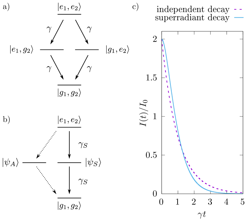
Figure 1: Level scheme for radiative decay in distinguishable (a) and superradiant (b) emitters. For ideal superradiance, $\gamma_{S}=2\gamma$ while transitions involving the antisymmetric Dicke state are completely dark. c) Time dependence of emitted intensity for cases (a) and (b) assuming an initially prepared doubly excited state $|e_{1},e_{2}\rangle$.

The cascaded emission through the superradiant three-level system also leads to a distinct non-exponential dynamics of the emitted intensity after excitation of the doubly excited state as depiced in Fig. 1c (cf. Appendix E or Ref. 16 for explicit expressions).

Finally, to assess signatures of superradiance on optical signals, the photon detection process has to be modelled. A point-like detector in the far field at a displacement $\boldsymbol{\mathcal{D}}$ with respect to the center of the emitters picks up only photons with a fixed wave vector $\mathbf{k}$ whose direction is parallel to $\boldsymbol{\mathcal{D}}$ and whose magnitude is determined by the detected energy $\hbar\omega=\hbar c|\mathbf{k}|$. The detected intensity signal is given by

$$I_{\mathbf{k}}(t)= \frac{1}{\Delta\tau_{M}}\langle a^{\dagger}_{\mathbf{k}}(t)a_{\mathbf{k}}(t)\rangle,$$ (5)

where $\Delta\tau_{M}$ is a characteristic timescale of the measurement, which depends on the detector (cf. discussion in Appendix A). Then, the time integral $\int_{t_{0}}^{t}dt^{\prime}\,I_{\mathbf{k}}(t^{\prime})$ yields the expectation value of the number of clicks on the detector from time $t_{0}$ to time $t$.

A finite-size detector is described by a collection of point-like detectors using the mask function $\eta_{\mathbf{k}}$, which is $\eta_{\mathbf{k}}=1$ for wave numbers $\mathbf{k}$ that are picked up by the detector and $\eta_{\mathbf{k}}=0$ otherwise. The corresponding intensity signal is

$$I(t)= \sum_{\mathbf{k}}\frac{\eta_{\mathbf{k}}}{\Delta\tau_{M}}\langle a^{\dagger}_{\mathbf{k}}(t)a_{\mathbf{k}}(t)\rangle$$ (6)

Similarly, photon coincidences are given by

$$G^{(2)}(t,\tau)= \sum_{\mathbf{k}\mathbf{k}^{\prime}}\frac{\eta_{\mathbf{k}}\eta_{\mathbf{k}^{\prime}}}{\Delta\tau_{M}^{2}}\langle a^{\dagger}_{\mathbf{k}}(t)a^{\dagger}_{\mathbf{k^{\prime}}}(t+\tau)a_{\mathbf{k}^{\prime}}(t+\tau)a_{\mathbf{k}}(t)\rangle,$$ (7)

$$g^{(2)}(t,\tau)= \frac{G^{(2)}(t,\tau)}{I(t)I(t+\tau)},$$ (8)

for unnormalized and normalized photon coincidences, respectively.

In Appendix A, we derive in detail how the photon emission can be expressed in terms of the state of the emitter system for cases of distinguishable and indistinguishable emitters. Defining the occupations of the states $|e_{1},e_{2}\rangle$, $|e_{1},g_{2}\rangle$, $|g_{1},e_{2}\rangle$, and $|\psi_{S}\rangle$, as $n_{e_{1},e_{2}}$, $n_{e_{1},g_{2}}$, $n_{g_{1},e_{2}}$, and $n_{S}$, respectively, the intensities from distinguishable and superradiant emitters are

$$I_{\textnormal{dist}}= I_{0}\sum_{i=1,2}\langle\sigma^{+}_{i}\sigma^{-}_{i}\rangle=I_{0}(2n_{e_{1},e_{2}}+n_{e_{1},g_{2}}+n_{g_{1},e_{2}}),$$ (9)

$$I_{\textnormal{sup}}= 2I_{0}\langle\sigma^{+}_{S}\sigma^{-}_{S}\rangle=2I_{0}(n_{e_{1},e_{2}}+n_{S}),$$ (10)

respectively, where $I_{0}=\sum_{\mathbf{k}}\eta_{\mathbf{k}}\gamma_{\mathbf{k}}^{\textnormal{single}}$ and $\gamma_{\mathbf{k}}^{\textnormal{single}}={2\pi}{\hbar}g^{2}_{\mathbf{k}}\delta(\hbar\omega_{\mathbf{k}}-\hbar\omega)$ is the rate of photon emission from a single emitter into the photon mode with wave vector $\mathbf{k}$ derived in Appendix A.

The corresponding coincidences are

$$G^{(2)}_{\textnormal{dist}}(t,\tau)= I_{0}^{2}\sum_{i,j=1,2}\langle\sigma^{+}_{i}(t)\sigma^{+}_{j}(t+\tau)\sigma^{-}_{j}(t+\tau)\sigma^{-}_{i}(t)\rangle,$$ (11)

$$G^{(2)}_{\textnormal{sup}}(t,\tau)= 4I_{0}^{2}\,\langle\sigma^{+}_{S}(t)\sigma^{+}_{S}(t+\tau)\sigma^{-}_{S}(t+\tau)\sigma^{-}_{S}(t)\rangle.$$ (12)

The normalized zero-delay coincidences $g^{(2)}(t,0)$ can be obtained noting that for the distinguishable case $\sigma^{-}_{i}\sigma^{-}_{i}=0$ while $\sigma^{-}_{j\neq i}\sigma^{-}_{i}=|g_{1},g_{2}\rangle\langle e_{1},e_{2}|$, so that

$$g^{(2)}_{\textnormal{dist}}(t,0)= \frac{2n_{e_{1},e_{2}}(t)}{\big{(}2n_{e_{1},e_{2}}(t)+n_{e_{1},g_{2}}(t)+n_{g_{1},e_{2}}(t)\big{)}^{2}},$$ (13)

which, for initially uncorrelated emitters with excited state populations $n_{1}$ and $n_{2}$, respectively, becomes

$$g^{(2)}_{\textnormal{dist}}(t,0)= \frac{2n_{1}(t)n_{2}(t)}{\big{(}n_{1}(t)+n_{2}(t)\big{)}^{2}}\leq\frac{1}{2},$$ (14)

where $g^{(2)}_{\textnormal{dist}}(t,0)=1/2$ for equally excited emitters $n_{1}(t)=n_{2}(t)$ with identical dipoles.

Eq. (14) sets the limit for photon coincidences from two independent emitters without involvement of correlations between the emitters, irrespective of the driving or other system parameters. As discussed in more detail in Appendix B, a violation of Eq. (14) constitutes a clear signature of cooperative effects, which requires emitters to be correlated at some point during the photon emission.

For superradiant emitters, $\sigma^{-}_{S}\sigma^{-}_{S}=|g_{1},g_{2}\rangle\langle e_{1},e_{2}|$, so the zero-delay coincidences are

$$g^{(2)}_{\textnormal{sup}}(t,0)= \frac{n_{e_{1},e_{2}}(t)}{\big{(}n_{e_{1},e_{2}}(t)+n_{S}(t)\big{)}^{2}},$$ (15)

which, for initially uncorrelated and equally occupied emitter states becomes $g^{(2)}_{\textnormal{sup}}(t,0)=1$, a value that is twice as large as the limit Eq. (14) for emission without cooperative effects.

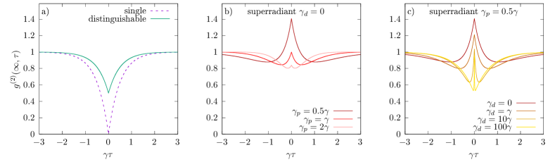
Figure 2: Photon coincidences $g^{(2)}(t,\tau)$ from the stationary state ($t\to\infty$) of continuously and incoherently pumped emitters for a) a single emitter and two distinguishable emitters (for $\gamma_{p}=\gamma$) and b) two superradiant emitters with superradiant decay rate $\gamma_{S}=2\gamma$ and different pump rates $\gamma_{p}$ without additional dephasing $\gamma_{d}=0$. c) Superradiant emission from two emitters with additional local dephasing $\gamma_{d}$ at pump rate $\gamma_{p}=0.5\gamma$.

Typically, photon coincidences are measured as a function of the delay time $\tau$, which additionally includes information about the dynamics. As long as the photon environment is not strongly structured as, e.g., in single-mode microcavities, and, hence, does not show significant non-Markovian memory effects, the time evolution can be well described by Lindblad master equations. For single, distinguishable, and superradiant emitters, which are pumped incoherently, the respective master equations are

$$\frac{\partial}{\partial t}\rho_{\textnormal{single}}= \gamma_{p}\mathcal{D}\big{[}\sigma^{+}_{1}\big{]}\big{(}\rho_{\textnormal{single}}\big{)}+\gamma\mathcal{D}\big{[}\sigma^{-}_{1}\big{]}\big{(}\rho_{\textnormal{single}}\big{)},$$ (16)

$$\frac{\partial}{\partial t}\rho_{\textnormal{dist}}= \gamma_{p}\mathcal{D}\big{[}\sigma^{+}_{1}\big{]}\big{(}\rho_{\textnormal{dist}}\big{)}+\gamma_{p}\mathcal{D}\big{[}\sigma^{+}_{2}\big{]}\big{(}\rho_{\textnormal{dist}}\big{)}$$

$$+\gamma\mathcal{D}\big{[}\sigma^{-}_{1}\big{]}\big{(}\rho_{\textnormal{dist}}\big{)}+\gamma\mathcal{D}\big{[}\sigma^{-}_{2}\big{]}\big{(}\rho_{\textnormal{dist}}\big{)},$$ (17)

$$\frac{\partial}{\partial t}\rho_{\textnormal{sup}}= \gamma_{p}\mathcal{D}\big{[}\sigma^{+}_{1}\big{]}\big{(}\rho_{\textnormal{sup}}\big{)}+\gamma_{p}\mathcal{D}\big{[}\sigma^{+}_{2}\big{]}\big{(}\rho_{\textnormal{sup}}\big{)}$$

$$+\gamma_{d}\mathcal{D}\big{[}\sigma^{+}_{1}\sigma^{-}_{1}\big{]}\big{(}\rho_{\textnormal{sup}}\big{)}+\gamma_{d}\mathcal{D}\big{[}\sigma^{+}_{2}\sigma^{-}_{2}\big{]}\big{(}\rho_{\textnormal{sup}}\big{)}$$

$$+\gamma_{S}\mathcal{D}\big{[}\sigma^{-}_{S}\big{]}\big{(}\rho_{\textnormal{sup}}\big{)},$$ (18)

respectively, where

$$\mathcal{D}\big{[}L\big{]}\big{(}\rho\big{)}= L\rho L^{\dagger}-\frac{1}{2}\big{(}L^{\dagger}L\rho+\rho L^{\dagger}L\big{)}.$$ (19)

is the Lindblad superoperator, $\gamma$ is the radiative decay rate of a single emitter, $\gamma_{p}$ is the pump rate, and $\gamma_{S}=2\gamma$ is the superradiant decay rate. Additionally, in the superradiant case, we have introduced local dephasing rates $\gamma_{d}$, which also leads to the decay of inter-emitter correlations.

Generally, two-time correlation functions of the form $\langle a^{\dagger}_{\mathbf{k}}(t)a^{\dagger}_{\mathbf{k^{\prime}}}(t+\tau)a_{\mathbf{k}^{\prime}}(t+\tau)a_{\mathbf{k}}(t)\rangle$ are obtained using the quantum regression theorem[30, 31] by propagating a density matrix according to the respective Lindblad master equations up to time $t$. Applying the respective operators, one defines the unnormalized pseudo density matrices $\rho^{\prime}(0)=a_{\mathbf{k}}\rho(t)a^{\dagger}_{\mathbf{k}}$. The latter is then propagated using the same master equation for a time $\tau$, at which the correlation function is evaluated as $\langle a^{\dagger}_{\mathbf{k}}(t)a^{\dagger}_{\mathbf{k^{\prime}}}(t+\tau)$ $a_{\mathbf{k}^{\prime}}(t+\tau)a_{\mathbf{k}}(t)\rangle=\textrm{Tr}\big{[}a^{\dagger}_{\mathbf{k^{\prime}}}a_{\mathbf{k}^{\prime}}\rho^{\prime}(\tau)\big{]}$.

With this approach, the delay-time dependent coincidences $g^{(2)}(t,\tau)$ from the stationary state $t\to\infty$ can be calculated analytically for single and indistinguishable emitters as (cf. Appendix C)

$$g^{(2)}_{\textnormal{single}}(\infty,\tau)= 1-e^{-(\gamma+\gamma_{p})\tau},$$ (20)

$$g^{(2)}_{\textnormal{dist}}(\infty,\tau)= 1-\frac{1}{2}e^{-(\gamma+\gamma_{p})\tau}.$$ (21)

The coincidences for the superradiant case are calculated numerically.

The delay-time dependence of $g^{(2)}(\infty,\tau)$ for the three cases are depicted in Fig. 2. As predicted analytically, the coincidences for single and distinguishable emitters show a dip at $\tau=0$ with $g^{(2)}_{\textnormal{single}}(\infty,0)=0$ and $g^{(2)}_{\textnormal{dist}}(\infty,0)=1/2$, respectively. In contrast, coincidences in the superradiant case feature an anti-dip with values $g^{(2)}_{\textnormal{sup}}(\infty,0)>1/2$. The height of the anti-dip $g^{(2)}_{\textnormal{sup}}(\infty,0)$ depends on the driving conditions like the pump rate $\gamma_{p}$ as shown in Fig. 2b. In line with Eq. (15), $g^{(2)}_{\textnormal{sup}}(t,0)=1$ when the emitters are uncorrelated at time $t$. This is the case for the stationary state at special driving conditions $\gamma_{p}=\gamma=\gamma_{S}/2$. Alternatively, the stationary state becomes uncorrelated if correlations introduced by driving and losses are suppressed by strong dephasing. Indeed, as depicted in Fig. 2c, $g^{(2)}_{\textnormal{sup}}(\infty,0)$ approaches 1 with increasing dephasing rate $\gamma_{d}$.

III Cooperative emission beyond superradiance

So far, we have discussed distinguishable and superradiant emitters, which are limiting cases of the Hamiltonian in Eq. (1) where the phase factors $e^{\pm i\mathbf{k}\cdot\mathbf{r}}$ in the light-matter coupling are either irrelevant or unity. We now consider the more general regime of spectrally indistinguishable emitters where the condition for free-space superradiance, namely inter-emitter distances $r\ll\lambda$ being much smaller than wavelength of the light, is dropped. Then, the phase factors in the coupling play a crucial and non-trivial role. At the same time, the condition $\omega_{1}=\omega_{2}$ for spectrally indistinguishable emitters again precludes a straightforward application of non-degenerate perturbation theory to describe the emission process. Here, we solve this problem by describing the interaction with each light field mode labelled by its wave vector $\mathbf{k}$ as an independent decay channel. For each channel, a situation analogous to that in the superradiant case emerges. The overall dynamics then follows from interference between the individual decay processes.

III.1 Radiative decay

In analogy to the superradiant case, we express the interaction Hamiltonian as

$$H_{I}= \sum_{\mathbf{k}}\hbar\sqrt{2}g_{\mathbf{k}}\big{(}\sigma^{-}_{\mathbf{k}}a^{\dagger}_{\mathbf{k}}+\sigma^{+}_{\mathbf{k}}a_{\mathbf{k}}\big{)},$$ (22)

where we define the lowering and raising operators

$$\sigma^{-}_{\mathbf{k}}= \frac{1}{\sqrt{2}}\big{(}e^{i\mathbf{k}\cdot\mathbf{r}/2}\sigma^{-}_{1}+e^{-i\mathbf{k}\cdot\mathbf{r}/2}\sigma^{-}_{2}\big{)}$$ (23)

and $\sigma^{+}_{\mathbf{k}}=\big{(}\sigma^{-}_{\mathbf{k}}\big{)}^{\dagger}$, which describe transitions

$$\sigma^{-}_{\mathbf{k}}= |g_{1},g_{2}\rangle\langle\psi_{\mathbf{k}}|+|\psi_{\mathbf{k}}\rangle\langle e_{1},e_{2}|$$ (24)

through the intermediate state

$$|\psi_{\mathbf{k}}\rangle= \frac{1}{\sqrt{2}}\big{(}e^{-i\mathbf{k}\cdot\mathbf{r}/2}|e_{1},g_{2}\rangle+e^{i\mathbf{k}\cdot\mathbf{r}/2}|g_{1},e_{2}\rangle\big{)}.$$ (25)

Thus, for a fixed vector $\mathbf{k}$, the state $|\psi_{\mathbf{k}}\rangle$ plays a similar role as the symmetric Dicke state $|\psi_{S}\rangle$ in the superradiant case (compare Fig. 3a with Fig. 1b), albeit with different intermediate states $|\psi_{\mathbf{k}}\rangle$ and $|\psi_{\mathbf{k}^{\prime}}\rangle$ for different wave vectors $\mathbf{k}$ and $\mathbf{k}^{\prime}$. Each wave vector $\mathbf{k}$ constitutes a decay channel from the doubly excited state to the ground state via an intermediate state $|\psi_{\mathbf{k}}\rangle$, which is described by a Lindblad term $\gamma_{\mathbf{k}}\mathcal{D}\big{[}\sigma^{-}_{\mathbf{k}}\big{]}\big{(}\rho\big{)}$ with rate (cf. Appendix A)

$$\gamma_{\mathbf{k}}={4\pi}{\hbar}g^{2}_{\mathbf{k}}\delta(\hbar\omega_{\mathbf{k}}-\hbar\omega_{i}).$$ (26)

This description serves several purposes: On the one hand, the decay channels characterize the extraction of $\mathbf{k}$-dependent emitted intensities and, thus, links the radiation pattern to the quantum state of the emitter system. On the other hand, due to conservation of excitations, the free radiative decay of the emitter system can be obtained by summing over the Lindbladians of all decay channels

$$\frac{\partial}{\partial t}\rho= \sum_{\mathbf{k}}\gamma_{\mathbf{k}}\Big{(}\sigma^{-}_{\mathbf{k}}\rho\sigma^{+}_{\mathbf{k}}-\frac{1}{2}(\sigma^{+}_{\mathbf{k}}\sigma^{-}_{\mathbf{k}}\rho+\rho\sigma^{+}_{\mathbf{k}}\sigma^{-}_{\mathbf{k}})\Big{)}.$$ (27)

With the concrete expressions for operators $\sigma^{\pm}_{\mathbf{k}}$ in Eq. (23), we can alternatively write this master equation

$$\frac{\partial}{\partial t}\rho= \gamma_{\textrm{sup}}\mathcal{D}\big{[}\sigma_{S}^{-}\big{]}\big{(}\rho\big{)}+\gamma_{\textrm{ind}}\Big{[}\mathcal{D}\big{[}\sigma_{1}^{-}\big{]}\big{(}\rho\big{)}+\mathcal{D}\big{[}\sigma_{2}^{-}\big{]}\big{(}\rho\big{)}\Big{]}$$ (28)

in terms of effective decay channels of the form of superradiant and independent decay, respectively, with rates

$$\gamma_{\textrm{sup}}= \sum_{\mathbf{k}}\gamma_{\mathbf{k}}e^{i\mathbf{k}\cdot\mathbf{r}},$$ (29)

$$\gamma_{\textrm{ind}}= \sum_{\mathbf{k}}\gamma_{\mathbf{k}}\frac{1}{2}\big{(}1-e^{i\mathbf{k}\cdot\mathbf{r}}\big{)}=\gamma-\frac{1}{2}\gamma_{\textrm{sup}},$$ (30)

where $\gamma$ is again the radiative decay rate of a single emitter.

Ignoring the radiation pattern of the dipole, i.e., assuming $\mathbf{k}$-independent couplings $g_{\mathbf{k}}=g$, integration over $\mathbf{k}$ yields

$$\gamma_{\textrm{sup}}= 2\gamma\frac{\sum_{\mathbf{k}}\delta(\hbar\omega_{\mathbf{k}}-\hbar\omega)e^{i\mathbf{k}\cdot\mathbf{r}}}{\sum_{\mathbf{k}}\delta(\hbar\omega_{\mathbf{k}}-\hbar\omega)}=2\gamma\frac{\sin(kr)}{kr}.$$ (31)

Including dipole radiation of identical emitters by accounting for light polarization $\mathbf{e}_{\mathbf{k},\lambda}\perp\mathbf{k}$ perpendicular to the wave propagation via $g_{\mathbf{k,\lambda}}=g(\hat{\mathbf{d}}\cdot\mathbf{e}_{\mathbf{k},\lambda})^{2}$, where $\hat{\mathbf{d}}$ denotes the normalized direction of the dipoles, and summing over $\lambda=1,2$ yields[16, 32]

$$\gamma_{\textrm{sup}}= 3\gamma\bigg{\{}\bigg{[}1-\frac{(\hat{\mathbf{d}}\cdot{\mathbf{r}})^{2}}{r^{2}}\bigg{]}\frac{\sin kr}{kr}$$

$$+\bigg{[}1-3\frac{(\hat{\mathbf{d}}\cdot{\mathbf{r}})^{2}}{r^{2}}\bigg{]}\bigg{[}\frac{\cos kr}{(kr)^{2}}-\frac{\sin kr}{(kr)^{3}}\bigg{]}\bigg{\}}.$$ (32)

For simplicity, here, we focus on the situation of dipoles tilted by an angle $\theta_{m}\approx 54.74^{\circ}$ with respect to the distance vector between the emitters, where $(\hat{\mathbf{d}}\cdot{\mathbf{r}})^{2}/r^{2}=\cos^{2}\theta_{m}=1/3$, where Eq. (31) is obtained as a special case of Eq. (32).

In this case, it is particularly clear that the master equation (28) reproduces the radiative decay terms in Eqs. (II) and (II) in the respective limits $r\gg\lambda$, where $\gamma_{\textnormal{ind}}=\gamma$ and $\gamma_{\textnormal{sup}}=0$, and $r\ll\lambda$, where $\gamma_{\textnormal{ind}}=0$ and $\gamma_{S}=\gamma_{\textnormal{sup}}=2\gamma$.

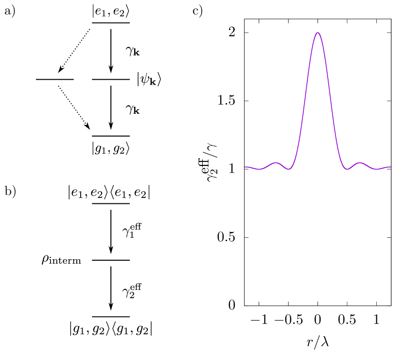
Figure 3: a) Radiative decay processes for general indistinguishable emitters involving a single photon wave vector $\mathbf{k}$ and b) its overall effect using a density matrix description. c) Effective emission rate $\gamma_{2}^{\textnormal{eff}}$ of the second photon as a function of the distance $r$ between the emitters for detection angle $\theta_{m}\approx 54.74^{\circ}$.

The net effect of the master equation (28) for a system initially prepared in the doubly excited state $|e_{1},e_{2}\rangle$ can be visualized (cf. Fig. 3b) as transitions involving an intermediate state expressed as a mixed-state density matrix $\rho_{\textnormal{interm}}$. This is obtained by equating the r.h.s. of Eq. (28) evaluated for $\rho=|e_{1},e_{2}\rangle\langle e_{1},e_{2}|$ with $\gamma_{1}^{\textnormal{eff}}\rho_{\textnormal{interm}}$, where $\rho_{\textnormal{interm}}$ is normalized to trace 1 and the norm defines the effective first photon emission rate $\gamma_{1}^{\textnormal{eff}}$. This yields

$$\rho_{\textnormal{interm}}= \sum_{\mathbf{k}}\frac{\gamma_{\mathbf{k}}}{2\gamma}|\psi_{\mathbf{k}}\rangle\langle\psi_{\mathbf{k}}|$$

$$= \frac{1}{2}\Big{[}|e_{1},g_{2}\rangle\langle e_{1},g_{2}|+|g_{1},e_{2}\rangle\langle g_{1},e_{2}|$$

$$+\frac{\sin(kr)}{kr}\big{(}|e_{1},g_{2}\rangle\langle g_{1},e_{2}|+|g_{1},e_{2}\rangle\langle e_{1},g_{2}|\big{)}\Big{]}.$$ (33)

The first photon emission rate $\gamma_{1}^{\textnormal{eff}}=2\gamma$, irrespective of the distance between emitters. The emission of a second photon from the intermediate state, on the other hand, depends on the overlap of the intermediate state with the respective decay channel

$$\gamma_{2}^{\textnormal{eff}}= \sum_{\mathbf{k}}\gamma_{\mathbf{k}}\langle\psi_{\mathbf{k}}|\rho_{\textnormal{interm}}|\psi_{\mathbf{k}}\rangle=\gamma\bigg{[}1+\Big{(}\frac{\sin(kr)}{kr}\Big{)}^{2}\bigg{]}.$$ (34)

The effective second photon emission rate $\gamma_{2}^{\textnormal{eff}}$ is shown in Fig. 3c as a function of the distance between the emitters. For small distances $r\ll\lambda$, one recovers the superradiant limit with $\gamma_{2}^{\textnormal{eff}}=\gamma_{1}^{\textnormal{eff}}=2\gamma$. At finite distances, the second photon emission rate decreases and eventually reaches values around $\gamma_{2}^{\textnormal{eff}}=\gamma_{1}^{\textnormal{eff}}/2=\gamma$ at $r\gtrsim\lambda/2$.

Thus, for large distances, the free radiative decay of two indistinguishable emitters behaves just like that of distinguishable or independent emitters, where two emitters can contribute to the first emission process, while, once one emitter is deexcited, only the remaining emitter contributes to the emission of the second photon. No sign of cooperative emission is found in this regime when only the free radiative decay is considered.

III.2 Photon coincidences

The reason why radiative decay alone does not lead to visible cooperative emission effects is related to the integration over all accessible light field modes (summation over $\mathbf{k}$). This situation changes markedly when $\mathbf{k}$-resolved quantities are considered[25, 24]. For example, measuring photon coincidences using two detectors, as depicted in Fig. 4, one usually collects photons emitted into a limited solid angle determined by the optical beam path as well as the position of the detectors relative to the emitters. Here, we assume two detectors with detection efficiencies $\eta_{\mathbf{k}}^{(1)}$ and $\eta_{\mathbf{k}}^{(2)}$ with finite support narrowly localized around reference wave vectors $\mathbf{k}_{0}^{(1)}$ and $\mathbf{k}_{0}^{(2)}$, respectively, i.e.,

$$\eta_{\mathbf{k}}^{(l)}=\begin{cases}\eta_{0},&\mathbf{k}\approx\mathbf{k}_{0}^{(l)},\\ 0,&\textnormal{else}.\end{cases}$$ (35)

The measured coincidence signal for wave-vector-selected photons can then be expressed as

$$g^{(2)}_{\textnormal{sel}}(t,\tau)= \frac{G^{(2)}_{\textnormal{sel}}(t,\tau)}{I_{\textnormal{sel}}(t)I_{\textnormal{sel}}(t+\tau)},$$ (36)

$$G^{(2)}_{\textnormal{sel}}(t,\tau)= \sum\limits_{\mathbf{k},\mathbf{k}^{\prime}=\mathbf{k}_{0}^{(1)},\mathbf{k}_{0}^{(2)}}\langle\sigma^{\dagger}_{\mathbf{k}}(t)\sigma^{\dagger}_{\mathbf{k}^{\prime}}(t+\tau)\sigma_{\mathbf{k}^{\prime}}(t+\tau)\sigma_{\mathbf{k}}(t)\rangle,$$ (37)

$$I_{\textnormal{sel}}(t)= \sum\limits_{\mathbf{k}=\mathbf{k}_{0}^{(1)},\mathbf{k}_{0}^{(2)}}\langle\sigma^{\dagger}_{\mathbf{k}}(t)\sigma_{\mathbf{k}}(t)\rangle.$$ (38)

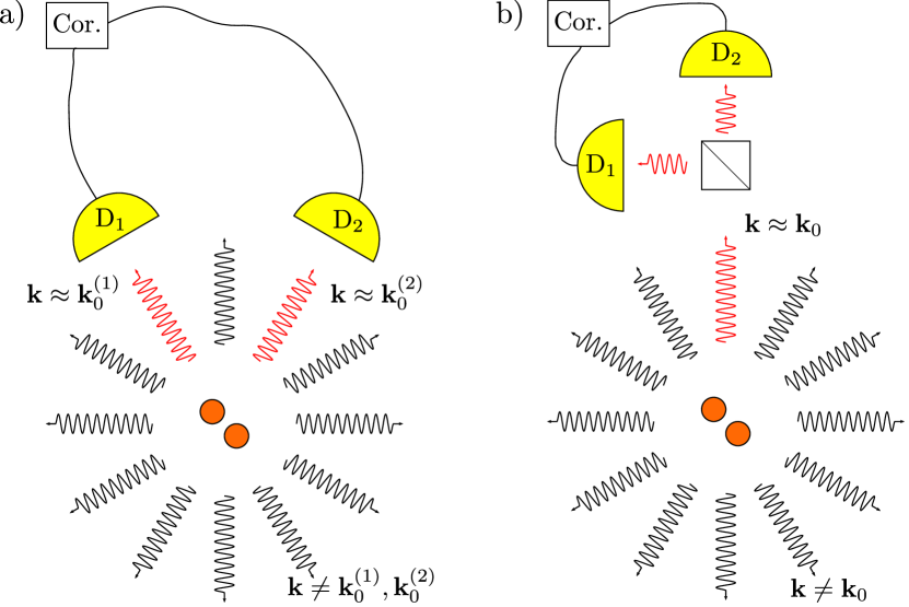
Figure 4: Sketch of photon coincidence setups. a) Coincidences recorded from two detectors. The detectors D₁ and D₂ predominantly register photons with wave vectors $\mathbf{k}$ close to reference wave vectors $\mathbf{k}_{0}^{(i)}$, which are determined by the relative positioning of the detectors with respect to the emitters. b) Hanbury Brown-Twiss setup measuring coincidences of photons in the same direction $\mathbf{k}_{0}^{(1)}=\mathbf{k}_{0}^{(2)}=\mathbf{k}_{0}$. Photons with different wave vectors $\mathbf{k}\neq\mathbf{k}_{0}^{(1)},\mathbf{k}_{0}^{(2)}$ are relevant for the dynamics as they take part in radiative decay processes, but do not contribute to the detected signals.

Because $\sigma_{\mathbf{k}_{0}^{(2)}}\sigma_{\mathbf{k}_{0}^{(1)}}=|g_{1},g_{2}\rangle\langle\psi_{\mathbf{k}_{0}^{(2)}}|\psi_{\mathbf{k}_{0}^{(1)}}\rangle\langle e_{1},e_{2}|$ with $\langle\psi_{\mathbf{k}_{0}^{(2)}}|\psi_{\mathbf{k}_{0}^{(1)}}\rangle=\cos\big{[}(\mathbf{k}_{0}^{(2)}-\mathbf{k}_{0}^{(1)})\cdot\mathbf{r}/2\big{]}$, the zero-delay coincidences become

$$g^{(2)}_{\textnormal{sel}}(t,0)= \bigg{(}\frac{3}{4}+\frac{1}{4}\cos\big{[}(\mathbf{k}_{0}^{(2)}-\mathbf{k}_{0}^{(1)})\cdot\mathbf{r}\big{]}\bigg{)}$$

$$\times\frac{4n_{e_{1},e_{2}}(t)}{\Big{(}2n_{e_{1},e_{2}}(t)+n_{\mathbf{k}_{0}^{(1)}}(t)+n_{\mathbf{k}_{0}^{(2)}}(t)\Big{)}^{2}},$$ (39)

where $n_{\mathbf{k}}=\langle\sigma^{\dagger}_{\mathbf{k}}\sigma_{\mathbf{k}}\rangle$ are the occupations of the state $|\psi_{\mathbf{k}}\rangle$. Note that the geometric factor $\big{(}1+\cos\big{[}(\mathbf{k}_{0}^{(2)}-\mathbf{k}_{0}^{(1)})\cdot\mathbf{r}\big{]}\big{)}$ can also be understood as interference of photons emitted from the two emitters much like in a double-slit experiment [26, 28, 29].

Specifically, for coincidence measurements with $\mathbf{k}_{0}^{(2)}=\mathbf{k}_{0}^{(1)}=\mathbf{k}_{0}$ as obtained by a Hanbury Brown-Twiss (HBT) setup [33] as depicted in Fig. 4b), one finds

$$g^{(2)}_{\textnormal{sel}}(t,0)= \frac{n_{e_{1},e_{2}}(t)}{\big{(}n_{e_{1},e_{2}}(t)+n_{\mathbf{k}_{0}}(t)\big{)}^{2}},$$ (40)

which is $g^{(2)}_{\textnormal{sel}}(t,0)=1$ for initially uncorrelated and equally occupied emitters. Notably, this result, which coincides with that for superradiant emitters, is independent of the distance $r$ between the dots and is therefore found even for $r\gtrsim\lambda$, where the free radiative decay shows no superradiant enhancement.

This finding can be understood as follows: Having detected a single photon from two indistinguishable emitters, no information is gained about the exact origin of the photon, i.e., whether it was emitted from emitter 1 or emitter 2. Consequently, when the system is initially in the doubly excited state, the detection event at detector 1 indicates a collapse of the wave function of the two-emitter system to the maximally entangled state $|\psi_{\mathbf{k}_{0}^{(1)}}\rangle$. In contrast to the situation for an uncorrelated statistical mixture of excitations in either emitter, emission of the second photon from the correlated state $|\psi_{\mathbf{k}_{0}^{(1)}}\rangle$ has an oscillator strength that strongly depends on the emission direction $\mathbf{k}_{0}^{(2)}$ of the second photon due to the overlap $\langle\psi_{\mathbf{k}_{0}^{(2)}}|\psi_{\mathbf{k}_{0}^{(1)}}\rangle=\cos\big{[}(\mathbf{k}_{0}^{(2)}-\mathbf{k}_{0}^{(1)})\cdot\mathbf{r}/2\big{]}$. Thus, the emission rate for the second photon in the direction $\mathbf{k}_{0}^{(2)}=\mathbf{k}_{0}^{(1)}$ is enhanced without a concomitant enhancement of the overall radiative decay rate by diverting oscillator strength from other emission directions $\mathbf{k}_{0}^{(2)}$, in particular from those for which $(\mathbf{k}_{0}^{(2)}-\mathbf{k}_{0}^{(1)})\cdot\mathbf{r}$ is close to an odd multiple of $\pi$, for which $g^{(2)}_{\textnormal{sel}}(t,0)\approx 0$. This gives rise to a distinct radiation pattern for photon coincidences, which has been measured in Refs. [24, 25].

Finally, it is noteworthy that, although the distance $r$ between the emitters is not relevant for the discussion of an ideal wave-vector-resolving HBT experiments ($\mathbf{k}_{0}^{(2)}=\mathbf{k}_{0}^{(1)}=\mathbf{k}_{0}$), there are practical limitations: A realistic detector picks up wave vectors $\mathbf{k}=\mathbf{k}_{0}+\delta\mathbf{k}$ in a finite range $\delta\mathbf{k}\in\Omega$ around the reference wave vector $\mathbf{k}_{0}$. Assuming that the detection efficiency $\eta_{\mathbf{k}}$ is constant and non-zero only in $\Omega$, the registration of a photon at the detector from an initially doubly excited two-emitter system can be described as a collapse of the system to the mixed state

$$\rho_{\textnormal{av}}= \frac{1}{2}\Big{[}|e_{1},g_{2}\rangle\langle e_{1},g_{2}|+|g_{1},e_{2}\rangle\langle g_{1},e_{2}|$$

$$+\xi|e_{1},g_{2}\rangle\langle g_{1},e_{2}|+\xi^{*}|g_{1},e_{2}\rangle\langle e_{1},g_{2}|\Big{]}$$ (41)

with

$$\xi= e^{-i\mathbf{k}_{0}\cdot\mathbf{r}}\int\limits_{\Omega}\frac{d\delta\mathbf{k}}{\Omega}e^{-i\delta\mathbf{k}\cdot\mathbf{r}}.$$ (42)

Consequently, the photon coincidences at zero delay for initially uncorrelated and equally occupied emitters are found to be

$$g^{(2)}_{\textnormal{av}}(t,0)= \frac{1+|\xi|^{2}}{2}.$$ (43)

$|\xi|^{2}$ can be regarded as a measure for the precision of the wave vector selection. As such, it determines how well cooperative effects of the emission from indistinguishable emitters are resolved by the detectors. Ideal detectors resolving single wave vectors $\mathbf{k}_{0}$ in a HBT setup produce $|\xi|^{2}=1$ and therefore $g^{(2)}(t,0)=1$, whereas for detectors with finite detection ranges $\Omega$, $|\xi|^{2}$ is reduced due to cancellation, which becomes significant for large distances $r\gtrsim 2\pi/\delta{k}_{\textnormal{max}}$, where $\delta k_{\textnormal{max}}$ is of the order of the maximal spread of wave vectors within the detectable range $\Omega$.

Thus, for realistic detectors and for large distances between the emitters, $\xi$ approaches 0 leading to zero-delay photon coincidence $g^{(2)}(t,0)=1/2$, similar to that for distinguishable emitters. This sets a natural limitation for the detection of cooperative effects, which is, however, much less stringent that the condition $r<\lambda$ for superradiance.

III.3 Delay-time dependence of photon coincidences

We now consider the delay-time dependence of photon coincidences in the case of an ideal HBT setup ($\mathbf{k}_{0}^{(2)}=\mathbf{k}_{0}^{(1)}=\mathbf{k}_{0}$, $|\xi|^{2}=1$) in the non-superradiant regime $r\gtrsim\lambda$ of cooperative emission by selective measurement. We assume continuously and incoherently driven identical emitters subject to radiative decay and additional dephasing with rate $\gamma_{d}$ (e.g., due to interactions with a phonon bath), whose free evolution is described by the Lindblad master equation

$$\frac{\partial}{\partial t}\rho_{\textnormal{sel}}= \gamma_{p}\mathcal{D}\big{[}\sigma_{1}^{+}\big{]}\big{(}\rho_{\textnormal{sel}}\big{)}+\gamma_{p}\mathcal{D}\big{[}\sigma_{2}^{+}\big{]}\big{(}\rho_{\textnormal{sel}}\big{)}$$

$$+\gamma_{d}\mathcal{D}\big{[}\sigma_{1}^{+}\sigma_{1}^{-}\big{]}\big{(}\rho_{\textnormal{sel}}\big{)}+\gamma_{d}\mathcal{D}\big{[}\sigma_{2}^{+}\sigma_{2}^{-}\big{]}\big{(}\rho_{\textnormal{sel}}\big{)}$$

$$+\gamma\mathcal{D}\big{[}\sigma_{1}^{-}\big{]}\big{(}\rho_{\textnormal{sel}}\big{)}+\gamma\mathcal{D}\big{[}\sigma_{2}^{-}\big{]}\big{(}\rho_{\textnormal{sel}}\big{)}.$$ (44)

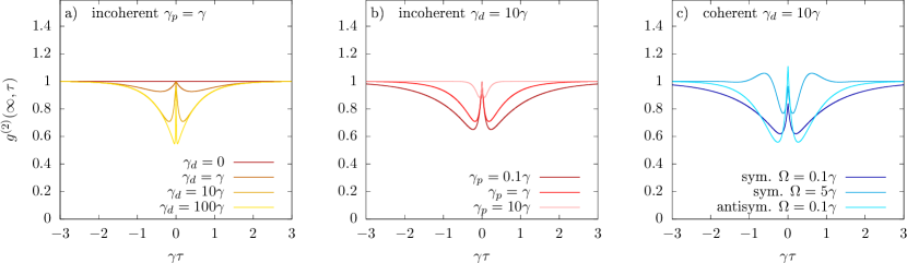
Figure 5: Delay-time dependence of photon coincidences $g^{(2)}(t\to\infty,\tau)$ for cooperative emission due to selective measurement. a) Coincidences for incoherent pumping with rate $\gamma_{p}=\gamma$ and for different dephasing rates $\gamma_{d}$. b) Incoherent pumping with different rates $\gamma_{p}$ at fixed dephasing rate $\gamma_{d}=10\gamma$. c) Coincidences for coherently driven indistinguishable emitters with dephasing rate $\gamma_{d}=10\gamma$ for different Rabi frequencies $\Omega$. The driving either couples to both emitters with the same phase (“sym.”) or with opposite phases (“antisym”).

The analysis can be simplified by considering identical emitters with identical occupations $n_{e_{1},g_{2}}=\langle e_{1},g_{2}|\rho|e_{1},g_{2}\rangle=\langle g_{1},e_{2}|\rho|g_{1},e_{2}\rangle=n_{g_{1},e_{2}}$ and choosing $e^{i\mathbf{k}_{0}\cdot\mathbf{r}}=1$. Note that, for fixed $\mathbf{k}_{0}$, a nonzero phase can be eliminated by redefining the phase of state $|e_{2}\rangle$. With this choice of phase, the only non-zero off-diagonal element of the 4-level density matrix, the inter-emitter coherences $c=\langle e_{1},g_{2}|\rho|g_{1},e_{2}\rangle$, remain real $c^{*}=c$ and the intermediate state $|\psi_{\mathbf{k}_{0}}\rangle$ coincides with the symmetric Dicke state $|\psi_{S}\rangle$. Furthermore, the trace condition $\textrm{Tr}(\rho)=1$ is used to express the ground state population as $n_{g_{1},g_{2}}=1-n_{e_{1},e_{2}}-2n_{e_{1},g_{2}}$. Noting further that the Lindblad master equation (44) never introduces coherences between states with different numbers of excitations, the dynamics can be fully described by the degrees of freedom $n_{e_{1},e_{2}},n_{e_{1},g_{2}},$ and $c$, which obey the equation of motion

$$\frac{\partial}{\partial t}\left(\begin{array}[]{c}n_{e_{1},e_{2}}\\ n_{e_{1},g_{2}}\\ c\end{array}\right)=A\left(\begin{array}[]{c}n_{e_{1},e_{2}}\\ n_{e_{1},g_{2}}\\ c\end{array}\right)+\left(\begin{array}[]{c}0\\ \gamma_{p}\\ 0\end{array}\right),$$ (54)

$$A=\left(\begin{array}[]{ccc}-2\gamma&2\gamma_{p}&0\\ (\gamma-\gamma_{p})&-\gamma-3\gamma_{p}&0\\ 0&0&-\gamma-\gamma_{p}-\gamma_{d}\end{array}\right).$$ (58)

First of all, we see that the coherences decouple from the dynamics of the remaining degrees of freedom and initial coherence $c(0)$, e.g., introduced by the measurement process, simply decay according to

$$c(t)= c(0)e^{-(\gamma+\gamma_{p}+\gamma_{d})t}.$$ (59)

The remaining two-dimensional linear inhomogeneous ordinary differential equation can, in principle, be solved analytically. Especially compact results are found in the special case of equal pumping and decay $\gamma_{p}=\gamma$, where the singly excited state population $n_{e_{1},g_{2}}$ is decoupled from the doubly excited state population $n_{e_{1},e_{2}}$. The corresponding equation

$$\frac{\partial}{\partial t}n_{e_{1},g_{2}}= -4\gamma n_{e_{1},g_{2}}+\gamma$$ (60)

is solved by

$$n_{e_{1},g_{2}}(t)= \frac{1}{4}+\Big{(}n_{e_{1},g_{2}}(0)-\frac{1}{4}\Big{)}e^{-4\gamma t}.$$ (61)

This expression acts as a driving term in the equation for the doubly excited state populations

$$\frac{\partial}{\partial t}n_{e_{1},e_{2}}= -2\gamma n_{e_{1},e_{2}}+2\gamma n_{e_{1},g_{2}},$$ (62)

which is solved by

$$n_{e_{1},e_{2}}(t)= \frac{1}{4}+\Big{(}n_{e_{1},e_{2}}(0)+n_{e_{1},g_{2}}(0)-\frac{1}{2}\Big{)}e^{-2\gamma t}$$

$$+\Big{(}\frac{1}{4}-n_{e_{1},g_{2}}(0)\Big{)}e^{-4\gamma t}.$$ (63)

Due to our choice of phase $e^{i\mathbf{k}_{0}\cdot\mathbf{r}}=1$, the optical signals are described by

$$G^{(2)}_{\textnormal{sel}}(t,\tau)= 4I_{0}^{2}\langle\sigma_{S}^{+}(t)\sigma_{S}^{+}(t+\tau)\sigma_{S}^{-}(t+\tau)\sigma_{S}^{-}(t)\rangle,$$ (64)

$$I_{\textnormal{sel}}(t)= 2I_{0}\langle\sigma_{S}^{+}(t)\sigma_{S}^{-}(t)\rangle$$

$$= 2I_{0}\big{(}n_{e_{1},e_{2}}(t)+n_{e_{1},g_{2}}(t)+c(t)\big{)},$$ (65)

where we have used $n_{S}=\frac{1}{2}(n_{e_{1},g_{2}}+n_{g_{1},e_{2}}+c+c^{*})=n_{e_{1},g_{2}}+c$.

To obtain the normalized coincidences $g^{(2)}_{\textnormal{sel}}(t,\tau)$ for emission from the stationary state at $t\to\infty$, $G^{(2)}_{\textnormal{sel}}(t\to\infty,\tau)$ and $I_{\textnormal{sel}}(t\to\infty)$ can be analyzed individually. First, observing that the Lindblad master equation (44) reduces coherences, one finds $c(t\to\infty)\to 0$, so the stationary intensity $I_{\textnormal{sel}}=2I_{0}(n_{e_{1},e_{2}}+n_{e_{1},g_{2}})=2I_{0}n_{e_{1}}$ becomes identical to $I_{\textnormal{dist}}$ for two distinguishable emitters.

Applying operators $\sigma_{S}^{\pm}$ at time $t$, one finds two nonzero contributions to the unnormalized coincidences $G^{(2)}_{\textnormal{sel}}(t,\tau)$ in Eq. (64): i) With probability $2I_{0}n_{e_{1},e_{2}}(t)$, a photon originating from the doubly excited state is detected. This measurement process leads to the collapse of the wave function to the state $|\psi_{S}\rangle$, which serves as the initial state for the delay-time propagation with $n^{\prime}_{e_{1},e_{2}}(\tau=0)=0$ and $n^{\prime}_{e_{1},g_{2}}(\tau=0)=c^{\prime}(\tau=0)=1/2$, where $n^{\prime}_{e_{1},e_{2}}$, $n^{\prime}_{e_{1},g_{2}}$, and $c^{\prime}$ refer to the occupations and coherences of the pseudo density matrix $\rho^{\prime}$ in the quantum regression theorem. ii) With probability $2I_{0}n_{S}(t)$, a photon originating from the single-excitation manifold is detected and the system collapses onto the ground state implying $n^{\prime}_{e_{1},e_{2}}(\tau=0)=n^{\prime}_{e_{1},g_{2}}(\tau=0)=c^{\prime}(\tau=0)=0$ for the delay-time propagation. In total, we find for $\gamma_{p}=\gamma$

$$g^{(2)}_{\textnormal{sel}}(\infty,\tau)= 1-\frac{1}{2}e^{-2\gamma\tau}+\underbrace{\frac{1}{2}|\xi|^{2}e^{-(\gamma+\gamma_{p}+\gamma_{d})\tau}}_{c^{\prime}(\tau)},$$ (66)

where we have re-introduced the factor $|\xi|^{2}\leq 1$ accounting for the finite range of wave vectors detected by a realistic detector.

It is noteworthy that the first two terms in Eq. (66) are identical to Eq. (21) for distinguishable emitters, which leads to a dip at $\tau\to 0$ with $g^{(2)}_{\textnormal{dist}}(\infty,0)=1/2$. Here, however, the last term in Eq. (66) provides an additive contribution that directly reflects the measurement-induced correlations $c^{\prime}(\tau)$ brought about by the collapse of the wave function due to photon detection from the doubly excited state and leaving the emitters in the correlated states $|\psi_{S}\rangle$. Perfect state preparation $|\xi|^{2}=1$, thus, leads to an anti-dip at $\tau\to 0$ with $g^{(2)}_{\textnormal{sel}}(\infty,0)=1$ and with a width determined by a combination of pump, decay, and dephasing rates.

While Eq. (66) is derived for the special driving condition of equal pump and decay rates $\gamma_{p}=\gamma$, a more comprehensive picture is gained by solving Eq. (44) numerically. In Fig. 5a and b, photon coincidences for the situation of cooperative emission due to selective measurement are depicted for different values of dephasing rates $\gamma_{d}$ (for $\gamma_{p}=\gamma$) and pumping rates $\gamma_{p}$ (for $\gamma_{d}=10\gamma$), respectively. In the absence of dephasing $\gamma_{d}=0$, coincidences remain $g^{(2)}(\infty,\tau)=1$ for all delay times $\tau$, which also follows from the cancellation of the second and the last terms in Eq. (66). For finite dephasing $\gamma_{d}\neq 0$, the cancellation is incomplete, effectively leading to an anti-dip similar to that observed in the superradiant case. The width of the anti-dip decreases with increasing dephasing rate. Increasing the pump rate $\gamma_{p}$ leads to a faster recovery of the stationary coincidences with values $g^{(2)}(\infty,\tau)=1$.

It is interesting to note that the zero-delay coincidences in Fig. 5a and b remain $g^{(2)}(\infty,0)=1$ for all dephasing rates $\gamma_{d}$ and pump rates $\gamma_{p}$. This is due to the fact that the zero-delay coincidences are fully determined by the stationary state and the measurement operators and do not probe dynamical aspects. Here, the stationary state is uncorrelated as the Lindblad master equation (44) contains no term introducing correlations. According to Eq. (40), this entails unity zero-delay coincidences. In contrast, the master equation (II) for the superradiant case includes the superradiant decay described by the operator $\sigma^{-}_{S}$, which does lead to correlations in the stationary state, hence deviations from $g^{(2)}(\infty,0)=1$ were found in Fig. 2.

However, non-unity values of the zero-delay coincidences may be obtained also in the case of cooperative emission in the absence of superradiance, as long as correlations in the stationary state are introduced by other means, e.g., by coherent driving of the two-emitter system. To demonstrate this, we present in Fig. 5c results for the coincidences obtained when the incoherent pumping is replaced by coherent driving described by the Hamiltonian

$$H_{\textnormal{sym}}= \frac{\hbar}{2}\Omega\big{[}(\sigma^{+}_{1}+\sigma^{-}_{1})+(\sigma^{+}_{2}+\sigma^{-}_{2})\big{]}$$ (67)

for driving of emitters with equal phases and

$$H_{\textnormal{antisym}}= \frac{\hbar}{2}\Omega\big{[}(\sigma^{+}_{1}+\sigma^{-}_{1})-(\sigma^{+}_{2}+\sigma^{-}_{2})\big{]}$$ (68)

for driving with opposite phases.

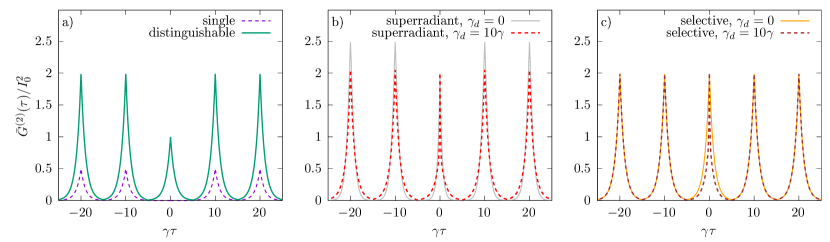
Figure 6: Delay-time dependence of photon coincidences $\bar{G}^{(2)}(\tau)$ after delta-like excitation with a pulse train with repetition time $T=10/\gamma$ for a) single and two distinguishable emitters, b) superradiant emitters without $\gamma_{d}=0$ and with dephasing $\gamma_{d}=10\gamma$, and c) cooperative emission due to selective measurement.

For weak coherent driving with equal phases, we find zero-delay coincidences $g^{(2)}_{\textnormal{sel}}(\infty,0)<1$. Increasing the driving strength eventually leads to shoulders at finite delay times indicative of Rabi oscillations, yet the zero-delay coincidences remain suppressed compared to incoherent pumping. However, weak driving with opposite phases indeed results in zero-delay coincidences exceeding one. This can again be explained by Eq. (40), which predicts that large values of coincidences are favoured by settings where the stationary occupations $n_{e_{1},e_{2}}\ll 1$ while still $n_{S}\ll n_{e_{1},e_{2}}$. Such a situation can be achieved by weakly driving the doubly excited state via the antisymmetric Dicke state $|\psi_{A}\rangle$.

III.4 Photon coincidences from pulsed driving

Beside continuous driving conditions, photon coincidences are also frequently investigated using pulsed laser excitation[34, 35], e.g., to assess the quality of on-demand single photon sources[36, 6, 7] or for quantum state tomography of sources of polarization-entangled photon pairs[37, 38]. In contrast to continuous driving, photon coincidences $G^{(2)}(t,\tau)$ under pulsed excitation depend explicitly on the detection time $t$ of the first photon. While suitably time-integrated and normalized coincidences agree with the zero-delay coindences obtained under continuous driving in the special cases of single and distinguishable emitters (see below), care has to be taken when interpreting more complex situations, where the results may differ drastically depending, e.g., on the choice of time integration windows[37, 38]. Therefore, we now derive photon coincidences under pulsed excitation for superradiant and cooperatively emitting emitters.

We consider emitters excited by a train of delta-like $\pi$-pulses with repetition time $T$. This time is chosen to be $T\gg 1/\gamma$ larger than the radiative decay time so that all excitations induced by one pulse have decayed before the next pulse arrives. Typically, one integrates over the arrival time $t$ of the first photon. The recorded histogram as a function of the delay time is proportional

$$\bar{G}^{(2)}(\tau):=\int\limits_{-T/2}^{T/2}dt\,G^{(2)}(t,\tau),$$ (69)

where we extend the domain of $\tau$ to negative delay times by setting $\bar{G}^{(2)}(-\tau)=\bar{G}^{(2)}(\tau)$.

The signal $\bar{G}^{(2)}(\tau)$ has the form of a series of distinct peaks as a function of the delay time $\tau$ as depicted in Fig. 6. The peak around $\tau=0$ originates from excitations during a single pulse. The peaks around $\tau=nT$ with integer $n\neq 0$ are due to excitations generated from different pulses. Hence, the peaks at $n\neq 0$ correspond to independent emission events and can be used as a normalization reference for photon coincidences of the zero-order peak.

There are two common ways to extract concrete figures of merit from the delay-time-dependent function $\bar{G}^{(2)}(\tau)$ given by i) the heights and ii) the integrals of the respective peaks. Both can be defined as

$$\bar{g}^{(2)}_{\Delta\tau}:= \frac{\bar{G}^{(2)}_{0,\Delta\tau}}{\bar{G}^{(2)}_{1,\Delta\tau}}.$$ (70)

in terms of the delay-time integral

$$\bar{G}^{(2)}_{n,\Delta\tau}:= \int\limits_{nT-\Delta\tau/2}^{nT+\Delta\tau/2}d\tau\,\bar{G}^{(2)}(\tau),$$ (71)

with delay-time integration window of width $\Delta\tau$. The peak heights (i) are obtained in the limit $\Delta\tau\to 0$, whereas the integrals over peaks (ii) are obtained for $\Delta\tau\to T$.

First, we focus on the calculation of $\bar{G}^{(2)}_{1,\Delta\tau}$ for peak $n=1$. The assumption $T\gg 1/\gamma$ implies that the first and second detected photons originate from different pulses and the emitters had relaxed to the ground state in the time between emission events. Thus, the states of the system at times $t$ and $t+\tau$ are uncorrelated, so correlation functions $\langle\sigma^{+}_{i}(t)\sigma^{+}_{j}(t+\tau)\sigma^{-}_{k}(t+\tau)\sigma^{-}_{l}(t)\rangle$ factorize into the product $\langle\sigma^{+}_{i}(t)\sigma^{-}_{l}(t)\rangle\langle\sigma^{+}_{j}(t+\tau)\sigma^{-}_{k}(t+\tau)\rangle$. Consequently,

$$G^{(2)}(t,t+\tau)=I(t)I(t+\tau),\quad\tau\gtrsim T$$ (72)

and one obtains

$$\bar{G}^{(2)}_{1,\Delta\tau\to 0}= \Delta\tau\int\limits_{0}^{T/2}dt\,I^{2}(t),$$ (73)

$$\bar{G}^{(2)}_{1,\Delta\tau\to T}= \bigg{[}\int\limits_{0}^{T/2}dt\,I(t)\bigg{]}^{2},$$ (74)

for short and long integration windows, respectively.

For the zeroth-order peak, the correlation functions have to be caculated explicitly as

$$\bar{G}^{(2)}_{0,\Delta\tau\to 0}= \Delta\tau\int\limits_{0}^{T/2}dt\,G^{(2)}(t,0)$$ (75)

$$\bar{G}^{(2)}_{0,\Delta\tau\to T}= 2\int\limits_{0}^{T/2}dt\int\limits_{0}^{T/2}d\tau\,G^{(2)}(t,\tau).$$ (76)

In the case of a single emitter (cf. Fig. 6a), the assumption of delta-like short pulses makes re-excitation impossible, so that at all times at most one excitation is present in the system. Hence, $G^{(2)}_{\textnormal{single}}(t,\tau)=0$ and also $\bar{g}^{(2)}_{\Delta\tau,\textnormal{single}}=0$, irrespective of the integration window and other details.

For two distinguishable emitters which are only subject to individual radiative decay (cf. Fig. 6a),

$$I_{\textnormal{dist}}(t)= 2I_{0}n(0)e^{-\gamma t},$$ (77)

$$G^{(2)}_{\textnormal{dist}}(t,\tau)= 2I_{0}^{2}n^{2}(0)e^{-\gamma t}e^{-\gamma(t+\tau)},$$ (78)

where $n(0)$ is the excited state occupation per emitter immediately after the pulse. This directly results in

$$\bar{g}^{(2)}_{\Delta\tau,\textnormal{dist}}=\frac{1}{2}$$ (79)

irrespective of the integration window $\Delta\tau$. The fact that this value coincides with $g^{(2)}_{\textnormal{dist}}(\infty,0)$ for continuously driven emitters is a direct consequence of the independent dynamics of both emitters and the effects of time-averaging being equal for numerator and denominator of Eq. (70), because the time-dependence of both is given by an exponential decay with the same rate.

However, the similarity between $\bar{g}^{(2)}_{\Delta\tau}$ and the zero-delay coincidences under continuous driving $g^{(2)}(\infty,0)$ does not carry over to cases with more complex dynamics. In Appendix D, we derive the integrated coincidences for two superradiant emitters in absence of additional dephasing

$$\bar{g}^{(2)}_{\Delta\tau\to 0,\textnormal{sup}}= \frac{n_{e_{1},e_{2}}(0)}{\frac{5}{4}n_{e_{1},e_{2}}^{2}(0)+\frac{1}{2}n_{S}^{2}(0)+\frac{3}{2}n_{e_{1},e_{2}}(0)n_{S}(0)},$$ (80)

$$\bar{g}^{(2)}_{\Delta\tau\to T,\textnormal{sup}}= \frac{2n_{e_{1},e_{2}}(0)}{\big{(}2n_{e_{1},e_{2}}(0)+n_{S}(0)\big{)}^{2}}.$$ (81)

Here, the values for different integration windows differ and are also not comparable to $g^{(2)}_{\textnormal{sup}}(\infty,0)$ for the continuously driven superradiant system derived in Eq. (15). This is primarily due to the non-exponential dynamics of the symmetric Dicke state occupations, which results in different time-averaging effects in numerator and denominator of $\bar{g}^{(2)}$. Note also that the results depend on the exact values of occupations of doubly excited and symmetric Dicke states created by the driving pulse. For example, if the doubly excited state is fully occupied, one finds $\bar{g}^{(2)}_{\Delta\tau\to 0,\textnormal{sup}}=\frac{4}{5}$ and $\bar{g}^{(2)}_{\Delta\tau\to T,\textnormal{sup}}=\frac{1}{2}$. The latter value is the same as for distinguishable emitters. Thus, $\bar{g}^{(2)}_{\Delta\tau\to T}$ fails to clearly indicate cooperative emission even for ideal superradiance.

In Fig. 6b, we present numerical calculations of $\bar{G}(\tau)$ in the superradiant case obtained using the master equations (II) without and with dephasing with rate $\gamma_{d}$, where, instead of pumping ($\gamma_{p}=0$), the state of the emitter is periodically reset to the doubly excited state with repetition time $T=10/\gamma$. Indeed, the ratio between the heights of the zeroth-order versus first-order peaks is $\bar{g}^{(2)}_{\Delta\tau\to 0,\textnormal{sup}}=1.25$ in the absence of dephasing. We have checked that the ratio between the integrals of the first and second peaks also reproduces the analytical value of $\bar{g}^{(2)}_{\Delta\tau\to T,\textnormal{sup}}=0.5$. It is noteworthy that numerical simulations with dephasing $\gamma_{d}=10\gamma$ reveal an increase of $\bar{g}^{(2)}_{\Delta\tau\to 0,\textnormal{sup}}$ extracted from the peak heights to a value of about $1.03$, while the ratio between the integrals remains the same $\bar{g}^{(2)}_{\Delta\tau\to T,\textnormal{sup}}=0.5$.

The time-integrated coincidences for the case of cooperative emission by selective measurement are derived in Appendix E. If the emitters are uncorrelated immediately after excitation, these reduce to

$$\bar{g}^{(2)}_{\Delta\tau\to 0,\textnormal{sel}}= 1,$$ (82)

$$\bar{g}^{(2)}_{\Delta\tau\to T,\textnormal{sel}}= \frac{1}{2}\bigg{[}1+\frac{\gamma}{\gamma+\gamma_{d}}\bigg{]}.$$ (83)

Here, we find that photon coincidences after pulsed excitation with short delay-time integration windows lead to similar results as $g^{(2)}_{\textnormal{sel}}(\infty,0)$ obtained under continuous driving. For wider windows, dephasing eventually reduces the integrated intensities, bringing it closer to the value of $\frac{1}{2}$ for independent emitters in the limit $\gamma_{d}\to\infty$. Numerically simulated $\bar{G}(\tau)$ depicted in Fig. 6c show that, in the absence of dephasing, the zeroth-order peak is identical to the first-order peak, hence $\bar{g}^{(2)}_{\Delta\tau\to 0,\textnormal{sel}}=\bar{g}^{(2)}_{\Delta\tau\to T,\textnormal{sel}}=1$. Dephasing with rate $\gamma_{d}=10\gamma$ only narrows the width of the zeroth-order peak, resulting in the same heights $\bar{g}^{(2)}_{\Delta\tau\to 0,\textnormal{sel}}=1$ but smaller integrals $\bar{g}^{(2)}_{\Delta\tau\to T,\textnormal{sel}}=\frac{6}{11}\approx 0.55<1$.

IV Discussion

We have investigated cooperative emission from two two-level quantum emitters, where both emitters contribute to both photon emission events. We compared two sources of cooperativity, superradiance and the preparation of correlated states by emission-angle-selective measurement. Superradiance and measurement-induced cooperativity require the emitters to be spectrally indistinguishable, but the former has stricter requirements in terms of spatial indistinguishabilty: A superradiant enhancement of the radiative decay rate necessitates that the electromagnetic environment cannot distinguish between emission from either dot. This can be achieved by confining emitters into regions much smaller than the wavelength of the emitted light[15, 16] or by exploiting photonic structures like waveguides[4, 21]. In contrast, measurement-induced cooperativity merely requires the detectors not to differentiate between photons from either dot, which depends more on the optical beam path than on the concrete spatial separation and, hence, can be found even when emitters in free space are separated by distances $r\gtrsim\lambda$ larger than the wavelength of the light.

The most tangible difference between the two forms of cooperative emission is that, in the case of superradiance, the radiative decay rate is enhanced, whereas the overall free decay rate after measurement-induced cooperativity remains the same as for independent emitters. However, the induced correlations shape the radiation pattern[24, 25], so that a second photon is more likely funnelled into the direction of the detectors at the expense of other emission directions. This difference makes both cases distinguishable via time-resolving measurements of the free radiative decay.

On the other hand, analyzing photon coincidences under continuous driving for superradiance as well as for cooperative emission due to selective measurement, we find that both have similar signatures on $g^{(2)}(\infty,\tau)$. In particular, in both cases, $g^{(2)}(\infty,\tau)$ has the form of an anti-dip, where zero-delay coincidences significantly exceed the limit of two independently emitting emitters $g^{(2)}(\infty,0)\leq\frac{1}{2}$. Thus, a violation of this limit is not a unique fingerprint for superradiance. Instead, it indicates more generally the involvement of correlations between emitters during the emission process, which provides the basis for the cooperation of both emitters in both photon emission processes.

Furthermore, although specifics of the system like driving and dephasing generally affect superradiance and cooperative emission due to selective measurement differently, the trends are subtle, which prohibits to clearly distinguish between both underlying mechanism of cooperative emission from the measured photon coincidences $g^{(2)}(\infty,\tau)$ alone.

The assessment of time-integrated coincidences $\bar{g}^{(2)}_{\Delta\tau}$ for emitters driven by short pulses reveals that these can serve as a proxy for instantaneous coincidences $g^{(2)}(\infty,0)$ for single and independent identical emitters. For measurement-induced cooperativity, this only holds for small delay-time integration windows $\Delta\tau$, because dephasing can have a large effect on signals time-integrated over wider windows. The situation is even more complex for spontaneously decaying superradiant emitters, where time-integration over the non-exponential dynamics obfuscates the relation to instantaneous coincidences $g^{(2)}(\infty,0)$.

Summarizing, we find that photon coincidence measurements can signal the presence of correlations between emitters in the decay process as an anti-dip in $g^{(2)}(t,\tau)$ as a function of $\tau$ with values of zero-delay coincidences $g^{(2)}(t,0)$ exceeding the limit for uncorrelated emitters. However, the origin of these correlations may be superradiance, cooperative emission without superradiance due to emission-angle-selective photon detection, or initial correlations induced by the driving. To clearly distinguish between these situation, additional information is required. A direct observation of a non-exponential behaviour of the overall emitted intensity is likely the most promising strategy to unambiguously prove the presence of superradiance.

Appendix A Microscopic derivation of $\mathbf{k}$-dependent emission and detection

Here, we show how photon observables for a single photon mode $\mathbf{k}$ such as $\langle a^{\dagger}_{\mathbf{k}}a_{\mathbf{k}}\rangle$ and the corresponding intensity $I_{\mathbf{k}}$ are related to emitter observables in Markovian emission processes induced by the light-matter interaction in the Hamiltonian in Eq. (1). This naturally leads to the picture that the interaction with light field mode $\mathbf{k}$ gives rise to a decay channel. From the Heisenberg equations of motion, it follows that

$$\frac{\partial}{\partial t}\langle a^{\dagger}_{\mathbf{k}}a_{\mathbf{k}}\rangle= \frac{i}{\hbar}\langle[H,a^{\dagger}_{\mathbf{k}}a_{\mathbf{k}}]\rangle$$

$$= -i\sqrt{2}g_{\mathbf{k}}\langle\sigma^{-}_{\mathbf{k}}a^{\dagger}_{\mathbf{k}}\rangle+i\sqrt{2}g_{\mathbf{k}}\langle\sigma^{+}_{\mathbf{k}}a_{\mathbf{k}}\rangle,$$ (84)

where we have used the definition of $\sigma_{\mathbf{k}}^{\pm}$ in Eq. (23). The light-matter correlations are determined by

$$\frac{\partial}{\partial t}\langle\sigma^{-}_{\mathbf{k}}a^{\dagger}_{\mathbf{k}}\rangle= i(\omega_{\mathbf{k}}-\omega)\langle\sigma^{-}_{\mathbf{k}}a^{\dagger}_{\mathbf{k}}\rangle+i\sqrt{2}g_{\mathbf{k}}\langle[\sigma^{+}_{\mathbf{k}}a_{\mathbf{k}},\sigma^{-}_{\mathbf{k}}a^{\dagger}_{\mathbf{k}}]\rangle$$

$$\approx i(\omega_{\mathbf{k}}-\omega)\langle\sigma^{-}_{\mathbf{k}}a^{\dagger}_{\mathbf{k}}\rangle+i\sqrt{2}g_{\mathbf{k}}\langle\sigma^{+}_{\mathbf{k}}\sigma^{-}_{\mathbf{k}}\rangle,$$ (85)

where we have simplified

$$\langle[\sigma^{+}_{\mathbf{k}}a_{\mathbf{k}},\sigma^{-}_{\mathbf{k}}a^{\dagger}_{\mathbf{k}}]\rangle= \langle\sigma^{+}_{\mathbf{k}}\sigma^{-}_{\mathbf{k}}\rangle+\langle[\sigma^{+}_{\mathbf{k}}\sigma^{-}_{\mathbf{k}}-\sigma^{-}_{\mathbf{k}}\sigma^{+}_{\mathbf{k}}]a^{\dagger}_{\mathbf{k}}a_{\mathbf{k}}\rangle$$ (86)

by neglecting the second term involving higher-order contributions. Integrating the equation of motion for the light-matter correlations yields

$$\langle\sigma^{-}_{\mathbf{k}}a^{\dagger}_{\mathbf{k}}\rangle= i\sqrt{2}g_{\mathbf{k}}\int\limits_{-\infty}^{t}d\tau\,e^{i(\omega_{\mathbf{k}}-\omega)(t-\tau)}\langle\sigma^{+}_{\mathbf{k}}\sigma^{-}_{\mathbf{k}}(\tau)\rangle$$

$$\approx i\sqrt{2}g_{\mathbf{k}}\pi\delta(\omega_{\mathbf{k}}-\omega)\langle\sigma^{+}_{\mathbf{k}}\sigma^{-}_{\mathbf{k}}\rangle,$$ (87)

where we have used the Markov approximation $\langle\sigma^{+}_{\mathbf{k}}\sigma^{-}_{\mathbf{k}}(\tau)\rangle\approx\langle\sigma^{+}_{\mathbf{k}}\sigma^{-}_{\mathbf{k}}(t)\rangle$ and neglected the frequency renormalization, i.e. the imaginary part of

$$\int\limits_{-\infty}^{t}d\tau\,e^{i(\omega-\omega_{\mathbf{k}})(\tau-t)}=\pi\delta(\omega-\omega_{\mathbf{k}})-\frac{i}{\omega-\omega_{\mathbf{k}}}.$$ (88)

Using $\langle\sigma^{-}_{\mathbf{k}}a^{\dagger}_{\mathbf{k}}\rangle=\langle\sigma^{+}_{\mathbf{k}}a_{\mathbf{k}}\rangle^{*}$, we arrive at the equation of motion for photon observables

$$\frac{\partial}{\partial t}\langle a^{\dagger}_{\mathbf{k}}a_{\mathbf{k}}\rangle= \gamma_{\mathbf{k}}\langle\sigma^{+}_{\mathbf{k}}\sigma^{-}_{\mathbf{k}}\rangle$$ (89)

with rate

$$\gamma_{\mathbf{k}}= 2\pi\hbar\,2g^{2}_{\mathbf{k}}\delta(\hbar\omega_{\mathbf{k}}-\hbar\omega).$$ (90)

Applying the same steps to the situation of a single emitter, where the interaction Hamiltonian is $\sum_{\mathbf{k}}\hbar g_{\mathbf{k}}(\sigma^{-}a^{\dagger}_{\mathbf{k}}+\sigma^{+}a_{\mathbf{k}})$, one obtains a similar result but with a rate

$$\gamma_{\mathbf{k}}^{\textnormal{single}}={2\pi}\hbar g^{2}_{\mathbf{k}}\delta(\hbar\omega_{\mathbf{k}}-\hbar\omega),$$ (91)

which is half of $\gamma_{\mathbf{k}}$ in Eq. (90).

For two spectrally distinguishable emitters, one has to account for two different light-matter correlations $\langle\sigma_{1}^{-}a^{\dagger}_{\mathbf{k}}\rangle$ and $\langle\sigma_{1}^{-}a^{\dagger}_{\mathbf{k}}\rangle$ oscillating with different frequencies $(\omega_{\mathbf{k}}-\omega_{1})$ and $(\omega_{\mathbf{k}}-\omega_{2})$, resulting in

$$\frac{\partial}{\partial t}\langle a^{\dagger}_{\mathbf{k}}a_{\mathbf{k}}\rangle= \gamma_{\mathbf{k}}^{(1)}\langle\sigma^{+}_{1}\sigma^{-}_{1}\rangle+\gamma_{\mathbf{k}}^{(2)}\langle\sigma^{+}_{2}\sigma^{-}_{2}\rangle,$$ (92)

with

$$\gamma_{\mathbf{k}}^{(i)}={2\pi}{\hbar}g^{2}_{\mathbf{k}}\delta(\hbar\omega_{\mathbf{k}}-\hbar\omega_{i}),$$ (93)

In addition to the time evolution induced by the light-matter interaction and described by Eqs. (89) and Eqs (92), respectively, the dynamics of the photon mode occupations $\langle a^{\dagger}_{\mathbf{k}}a_{\mathbf{k}}\rangle$ is also affected by the destructive measurement at the detectors. We model the continuous destructive measurement of photons, e.g., using a single-photon detector[39], by a periodic projective measurement of $\langle a^{\dagger}_{\mathbf{k}}a_{\mathbf{k}}\rangle$ at time intervals with width $\Delta\tau_{M}$ corresponding to the time scale of the measurement, which is determined by characteristics of the detector, such as the timing jitter. The destructive character of the measurement implies that the photon state is reset to the vacuum state with $\langle a^{\dagger}_{\mathbf{k}}a_{\mathbf{k}}\rangle=0$ immediately after the measurement, irrespective of the outcome. The probability of detecting a photon per time interval $\Delta\tau_{M}$ with a point-like detector measuring photon mode $\mathbf{k}$ is, hence, determined by the accumulated excitation transfer from the emitter system

$$I_{\mathbf{k}}(t)= \frac{1}{\Delta\tau_{M}}\int\limits_{t}^{t+\Delta\tau_{M}}dt^{\prime}\;\bigg{(}\frac{\partial}{\partial t^{\prime}}\langle a^{\dagger}_{\mathbf{k}}(t^{\prime})a_{\mathbf{k}}(t^{\prime})\rangle\bigg{)}$$

$$\approx \frac{\partial}{\partial t}\langle a^{\dagger}_{\mathbf{k}}(t)a_{\mathbf{k}}(t)\rangle$$ (94)

where we have assumed that the source terms, i.e., the emitter occupations do not change noticably on the time scale $\Delta\tau_{M}$. Concretely, for single, two spectrally distinguishable, and two indistinguishable emitters, we arrive at

$$I_{\mathbf{k}}^{\textnormal{single}}(t)= \gamma_{\mathbf{k}}^{\textnormal{single}}\langle\sigma^{+}\sigma^{-}(t)\rangle,$$ (95)

$$I_{\mathbf{k}}^{\textnormal{dist}}(t)= \gamma_{\mathbf{k}}^{(1)}\langle\sigma^{+}_{1}\sigma^{-}_{1}(t)\rangle+\gamma_{\mathbf{k}}^{(2)}\langle\sigma^{+}_{2}\sigma^{-}_{2}(t)\rangle,$$ (96)

$$I_{\mathbf{k}}^{\textnormal{indist}}(t)= \gamma_{\mathbf{k}}\langle\sigma^{+}_{\mathbf{k}}\sigma^{-}_{\mathbf{k}}(t)\rangle,$$ (97)

respectively.

Appendix B Involvement of correlations when $g^{(2)}(t,0)>\frac{1}{2}$

We now show why, for a system of two emitters subject to Markovian emission processes, a violation of $g^{(2)}(t,0)\leq\frac{1}{2}$ indicates the presence of inter-emitter correlations.

Note that the derivation of this limit in Eq. (14) is based on two assumptions: i) Absence of initial correlations and ii) photon coincidences are given by Eq. (11), which is the expression for distinguishable emitter.

The former case i) trivially involves correlations. An example is a situation with $n_{e_{1},g_{2}}=n_{g_{1},e_{2}}=0$, where $g^{(2)}_{\textnormal{dist.}}(t,0)=1/(2{n_{e_{1},e_{2}}(t)})$. Then, photon coincidences can reach arbitrarily high values when $n_{e_{1},e_{2}}$ is small.

As discussed in Appendix A, ii) is valid for Markovian emission processes if the emitters are spectrally distinguishable. Thus, for ii) to break down, the emitters must have the same transition frequencies $\omega_{1}=\omega_{2}$. Because of the Markovian outcoupling as well as the conservation of the number of excitations, photon coincidences must be described as

$$G^{(2)}(t,\tau)\propto\sum_{j,j^{\prime}}\langle\varsigma_{j}^{+}(t)\varsigma_{j^{\prime}}^{+}(t+\tau)\varsigma_{j^{\prime}}^{-}(t+\tau)\varsigma_{j}^{-}(t)\rangle,$$ (98)

in terms of two pairs of raising and lowering operators $\varsigma_{j}^{\pm}$ with respect to the emitter state, which are linear combinations $\varsigma_{j}^{-}=\alpha_{j}\sigma_{1}^{-}+\beta_{j}\sigma_{2}^{-}$ and $\varsigma_{j}^{+}=\alpha^{*}_{j}\sigma_{1}^{+}+\beta^{*}_{j}\sigma_{2}^{+}$ of operators $\sigma^{\pm}_{1}$ and $\sigma^{\pm}_{2}$ for the first and second emitter, respectively (Compare with Appendix A). If, for all contributions $j$, either $\alpha_{j}$ or $\beta_{j}$ are zero, one recovers Eq. (11). Thus, the only situation that remains to be discussed is that where there is at least one $j$ for which $\varsigma_{j}^{-}$ is a genuine linear combination of $\sigma^{-}_{1}$ and $\sigma^{-}_{2}$ with both $\alpha_{j}$ and $\beta_{j}$ nonzero.

Noting also that a non-zero contribution to zero-delay coincidences $G^{(2)}(t,0)$ are due to occupations of the doubly excited state $n_{e_{1},e_{2}}$ due to conservation of the number of excitations, we observe that $\varsigma_{j}^{-}$ applied to $|e_{1},e_{2}\rangle$ yields

$$\varsigma_{j}^{-}|e_{1},e_{2}\rangle= \alpha_{j}|g_{1},e_{2}\rangle+\beta_{j}|e_{1},g_{2}\rangle.$$ (99)

As both $\alpha_{j}$ and $\beta_{j}$ are nonzero, the intermediate state after the emission of a first photon possesses finite inter-emitter correlations of magnitude $|\alpha_{j}\beta^{*}_{j}|$.

Thus, if $g^{(2)}(t,0)>\frac{1}{2}$, correlations are involved in the emission process in the initial state, in the intermediate state after the emission of the first photon, or both.

Appendix C Continuous incoherent pumping of single and distinguishable emitters

The excited state population $n_{i}$ of single emitter subject to radiative decay with rate $\gamma$ and incoherently pumped with a rate $\gamma_{p}$ can be described

$$\frac{\partial}{\partial t}n_{i}= \gamma_{p}(1-n_{i})-\gamma n_{i},$$ (100)

where $(1-n_{i})$ is the population of the ground state. This equation of motion is solved by

$$n_{i}(t)= \frac{\gamma_{p}}{\gamma+\gamma_{p}}+\bigg{[}n_{i}(0)-\frac{\gamma_{p}}{\gamma+\gamma_{p}}\bigg{]}e^{-(\gamma+\gamma_{p})t}.$$ (101)

Photon coincidences from a single emitter require the detection of a first photon at time $t$, which occurs with a probability $I_{0}n_{1}(t)$ and implies a collapse of the emitter state onto the ground state, which defines the initial value $n_{1}(\tau=0)=0$ for the propagation for the delay time $\tau$. Therefore,

$$G^{(2)}_{\textnormal{single}}(t,\tau)= I_{0}^{2}\langle\sigma_{1}^{+}(t)\sigma_{1}^{+}(t+\tau)\sigma_{1}^{-}(t+\tau)\sigma_{1}^{-}(t)\rangle$$

$$= I_{0}^{2}n_{1}(t)\frac{\gamma_{p}}{\gamma+\gamma_{p}}\Big{(}1-e^{-(\gamma+\gamma_{p})\tau}\Big{)}.$$ (102)

Evaluating the coincidences from the stationary state $t\to\infty$ and normalizing by the squared intensity $I_{0}^{2}(\infty)=I_{0}^{2}\big{[}\gamma_{p}/(\gamma_{p}+\gamma)\big{]}^{2}$, one obtains

$$g^{(2)}_{\textnormal{single}}(\infty,\tau)= 1-e^{-(\gamma+\gamma_{p})\tau}.$$ (103)

For two distinguishable emitters, the photon coincidences are

$$G^{(2)}_{\textnormal{dist}}(t,\tau)= I_{0}^{2}\sum_{i,j=1,2}\langle\sigma_{i}^{+}(t)\sigma_{j}^{+}(t+\tau)\sigma_{j}^{-}(t+\tau)\sigma_{i}^{-}(t)\rangle$$

$$= I_{0}^{2}\sum_{i}\langle\sigma_{i}^{+}(t)\sigma_{i}^{+}(t+\tau)\sigma_{i}^{-}(t+\tau)\sigma_{i}^{-}(t)\rangle$$

$$+I_{0}^{2}\sum_{i,j\neq i}\langle\sigma_{i}^{+}(t)\sigma_{i}^{-}(t)\rangle\langle\sigma_{j}^{+}(t+\tau)\sigma_{j}^{-}(t+\tau)\rangle$$

$$= 2G^{(2)}_{\textnormal{single}}(t,\tau)+2I_{\textnormal{single}}(t)I_{\textnormal{single}}(t+\tau).$$ (104)

With $I_{\textnormal{dist}}(t)=2I_{\textnormal{single}}(t)$, the normalized coincidences from the stationary state are

$$g^{(2)}_{\textnormal{dist}}(\infty,\tau)= 1-\frac{1}{2}e^{-(\gamma+\gamma_{p})\tau}.$$ (105)

Appendix D Time-integrated coincidences for superradiant emitters

We consider the free radiative decay of a superradiant two-emitter system after optical excitation without additional dephasing. The equations of motion for the occupations of the doubly excited state $n_{e_{1},e_{2}}$ and the symmetric Dicke state $n_{S}$ are

$$\frac{\partial}{\partial t}n_{e_{1},e_{2}}= -\gamma_{S}n_{e_{1},e_{2}},$$ (106)

$$\frac{\partial}{\partial t}n_{S}= \gamma_{S}(n_{e_{1},e_{2}}-n_{S}),$$ (107)

with superradiant rate $\gamma_{S}=2\gamma$. These equation are solved by

$$n_{e_{1},e_{2}}(t)= n_{e_{1},e_{2}}(0)e^{-\gamma_{S}t},$$ (108)

$$n_{S}(t)= \big{[}n_{S}(0)+\gamma_{S}t\,n_{e_{1},e_{2}}(0)\big{]}e^{-\gamma_{S}t}.$$ (109)

The instantaneous emitted intensity according to Eq. (10) is

$$I_{\textnormal{sup}}(t)= 2I_{0}\big{[}n_{e_{1},e_{2}}(t)+n_{S}(t)\big{]}$$

$$= 2I_{0}\big{[}n_{e_{1},e_{2}}(0)+n_{S}(0)+\gamma_{S}t\,n_{e_{1},e_{2}}(0)\big{]}e^{-\gamma_{S}t}.$$ (110)

With Eqs. (73) and (74), we find for the superradiant photon coincidences defined by Eq. (12)

$$\bar{G}^{(2)}_{1,\Delta\tau\to 0}= \Delta\tau 4I^{2}_{0}\frac{\frac{5}{2}n_{e_{1},e_{2}}^{2}(0)+3n_{e_{1},e_{2}}(0)n_{S}(0)+n_{S}^{2}(0)}{2\gamma_{S}},$$ (111)

$$\bar{G}^{(2)}_{1,\Delta\tau\to T}= 4I^{2}_{0}\bigg{[}\frac{2n_{e_{1},e_{2}}(0)+n_{S}(0)}{\gamma_{S}}\bigg{]}^{2}.$$ (112)

The only term contributing to coincidences is the initially doubly excited state occupation $n_{e_{1},e_{2}}$, which radiatively decays for time $t$, is then translated into occupations of the symmetric Dicke state $n_{S}$ by applications of operators $\sigma^{\pm}_{S}$, and subsequent decays from there. This results in

$$\bar{G}^{(2)}_{0,\Delta\tau\to 0}= \Delta\tau 4I^{2}_{0}\int\limits_{0}^{T/2}dt\,n_{e_{1},e_{2}}(0)e^{-\gamma_{S}t}$$

$$= \frac{\Delta\tau 4I^{2}_{0}}{\gamma_{S}}n_{e_{1},e_{2}}(0),$$ (113)

$$\bar{G}^{(2)}_{0,\Delta\tau\to T}= 8I^{2}_{0}\int\limits_{0}^{T/2}dt\int\limits_{0}^{T/2}d\tau\,n_{e_{1},e_{2}}(0)e^{-\gamma_{S}(t+\tau)}$$

$$= \frac{8I^{2}_{0}}{\gamma_{S}^{2}}n_{e_{1},e_{2}}(0).$$ (114)

Appendix E Time-integrated coincidences for selectively measured emitters

In the case of cooperative emission due to selective measurement with two identical emitter, the relevant quantities are the occupation of the doubly excited state $n_{e_{1},e_{2}}$, the occupation of exactly one site $n_{e_{1},g_{2}}=n_{g_{1},e_{2}}$ as well as the correlations $c$ between the states with exactly one excitation.

The equations of motion are

$$\frac{\partial}{\partial t}c= -(\gamma+\gamma_{d})c,$$ (115)

$$\frac{\partial}{\partial t}n_{e_{1},e_{2}}= -2\gamma n_{e_{1},e_{2}},$$ (116)

$$\frac{\partial}{\partial t}n_{e_{1},g_{2}}= -\gamma n_{e_{1},g_{2}}+\gamma n_{e_{1},e_{2}},$$ (117)

which are solved by

$$c(t)= c(0)e^{-(\gamma+\gamma_{d})t},$$ (118)

$$n_{e_{1},e_{2}}(t)= n_{e_{1},e_{2}}(0)e^{-2\gamma t},$$ (119)

$$n_{e_{1},g_{2}}(t)= \big{[}n_{e_{1},g_{2}}(0)+n_{e_{1},e_{2}}(0)\big{]}e^{-\gamma t}-n_{e_{1},e_{2}}(0)e^{-2\gamma t}.$$ (120)

The emitted intensity is

$$I_{\textnormal{sel.}}(t)= 2I_{0}\big{[}n_{e_{1},e_{2}}(t)+n_{e_{1},g_{2}}(t)+c(t)\big{]}$$

$$= 2I_{0}\bigg{[}\big{[}n_{e_{1},g_{2}}(0)+n_{e_{1},e_{2}}(0)\big{]}e^{-\gamma t}+c(0)e^{-(\gamma+\gamma_{d})t}\bigg{]},$$ (121)

which yields

$$\bar{G}^{(2)}_{1,\Delta\tau\to 0}= \Delta\tau 4I^{2}_{0}\bigg{[}\frac{\big{[}n_{e_{1},g_{2}}(0)+n_{e_{1},e_{2}}(0)\big{]}^{2}}{2\gamma}$$

$$+\frac{2\big{[}n_{e_{1},g_{2}}(0)+n_{e_{1},e_{2}}(0)\big{]}c(0)}{2\gamma+\gamma_{d}}+\frac{c^{2}(0)}{2\gamma+2\gamma_{d}}\bigg{]},$$ (122)

$$\bar{G}^{(2)}_{1,\Delta\tau\to T}= 4I_{0}^{2}\bigg{[}\frac{n_{e_{1},g_{2}}(0)+n_{e_{1},e_{2}}(0)}{\gamma}+\frac{c(0)}{\gamma+\gamma_{d}}\bigg{]}^{2}.$$ (123)

The coincidences are determined by the decay of $n_{e_{1},e_{2}}$ until time $t$, which is collapsed onto the symmetric Dicke state for which $n^{\prime}_{e_{1},g_{2}}(\tau=0)=c^{\prime}(\tau=0)=\frac{1}{2}n_{e_{1},e_{2}}(t)$. These occupations and correlations then decay for time $\tau$. This yields

$$\bar{G}^{(2)}_{0,\Delta\tau\to 0}= \Delta\tau 4I_{0}^{2}\frac{1}{2\gamma}n_{e_{1},e_{2}}(0),$$ (124)

$$\bar{G}^{(2)}_{0,\Delta\tau\to T}= 4I_{0}^{2}\frac{1}{2\gamma}n_{e_{1},e_{2}}(0)\bigg{[}\frac{1}{\gamma}+\frac{1}{\gamma+\gamma_{d}}\bigg{]}.$$ (125)

References

- Einstein [1916] A. Einstein, Verh. Deutsch. Phys. Ges. 18, 318 (1916).
- Weisskopf [1935] V. Weisskopf, Naturwissenschaften 23, 631 (1935).
- Drexhage et al. [1968] K. H. Drexhage, H. Kuhn, and F. P. Schäfer, Ber. Bunsenges. Phys. Chem 72, 329 (1968).
- Kim et al. [2018] J.-H. Kim, S. Aghaeimeibodi, C. J. K. Richardson, R. P. Leavitt, and E. Waks, Nano Letters 18, 4734 (2018).
- Jöns et al. [2017] K. D. Jöns, L. Schweickert, M. A. M. Versteegh, D. Dalacu, P. J. Poole, A. Gulinatti, A. Giudice, V. Zwiller, and M. E. Reimer, Scientific Reports 7, 1700 (2017).
- Thomas et al. [2021] S. E. Thomas, M. Billard, N. Coste, S. C. Wein, Priya, H. Ollivier, O. Krebs, L. Tazaïrt, A. Harouri, A. Lemaitre, I. Sagnes, C. Anton, L. Lanco, N. Somaschi, J. C. Loredo, and P. Senellart, Phys. Rev. Lett. 126, 233601 (2021).
- Cosacchi et al. [2019] M. Cosacchi, F. Ungar, M. Cygorek, A. Vagov, and V. M. Axt, Phys. Rev. Lett. 123, 017403 (2019).
- Liu et al. [2018] F. Liu, A. J. Brash, J. O’Hara, L. M. P. P. Martins, C. L. Phillips, R. J. Coles, B. Royall, E. Clarke, C. Bentham, N. Prtljaga, I. E. Itskevich, L. R. Wilson, M. S. Skolnick, and A. M. Fox, Nature Nanotechnology 13, 835 (2018).
- Leistikow et al. [2011] M. D. Leistikow, A. P. Mosk, E. Yeganegi, S. R. Huisman, A. Lagendijk, and W. L. Vos, Phys. Rev. Lett. 107, 193903 (2011).
- Iles-Smith et al. [2017] J. Iles-Smith, D. P. S. McCutcheon, A. Nazir, and J. Mørk, Nature Photonics 11, 521 (2017).
- del Valle et al. [2012] E. del Valle, A. Gonzalez-Tudela, F. P. Laussy, C. Tejedor, and M. J. Hartmann, Phys. Rev. Lett. 109, 183601 (2012).
- del Valle et al. [2011] E. del Valle, A. Gonzalez–Tudela, E. Cancellieri, F. P. Laussy, and C. Tejedor, New Journal of Physics 13, 113014 (2011).
- Seidelmann et al. [2019] T. Seidelmann, F. Ungar, M. Cygorek, A. Vagov, A. M. Barth, T. Kuhn, and V. M. Axt, Phys. Rev. B 99, 245301 (2019).
- Seidelmann et al. [2021] T. Seidelmann, M. Cosacchi, M. Cygorek, D. E. Reiter, A. Vagov, and V. M. Axt, Advanced Quantum Technologies 4, 2000108 (2021).
- Dicke [1954] R. H. Dicke, Phys. Rev. 93, 99 (1954).
- Gross and Haroche [1982] M. Gross and S. Haroche, Phys. Rep 93, 301 (1982).
- Bradac et al. [2017] C. Bradac, M. T. Johnsson, M. v. Breugel, B. Q. Baragiola, R. Martin, M. L. Juan, G. K. Brennen, and T. Volz, Nature Communications 8, 1205 (2017).
- Higgins et al. [2014] K. D. B. Higgins, S. C. Benjamin, T. M. Stace, G. J. Milburn, B. W. Lovett, and E. M. Gauger, Nature Communications 5, 4705 (2014).
- Yang et al. [2021] D. Yang, S.-h. Oh, J. Han, G. Son, J. Kim, J. Kim, M. Lee, and K. An, Nature Photonics 15, 272 (2021).
- Quach et al. [2022] J. Q. Quach, K. E. McGhee, L. Ganzer, D. M. Rouse, B. W. Lovett, E. M. Gauger, J. Keeling, G. Cerullo, D. G. Lidzey, and T. Virgili, Science Advances 8, eabk3160 (2022).
- Grim et al. [2019] J. Q. Grim, A. S. Bracker, M. Zalalutdinov, S. G. Carter, A. C. Kozen, M. Kim, C. S. Kim, J. T. Mlack, M. Yakes, B. Lee, and D. Gammon, Nature Materials 18, 963 (2019).
- Koong et al. [2022] Z. X. Koong, M. Cygorek, E. Scerri, T. S. Santana, S. I. Park, J. D. Song, E. M. Gauger, and B. D. Gerardot, Science Advances 8, eabm8171 (2022).
- Note [1] This is because in absence of correlations for and for . Hence and . This expression is maximal for equal , for which .
- Wolf et al. [2020] S. Wolf, S. Richter, J. von Zanthier, and F. Schmidt-Kaler, Phys. Rev. Lett. 124, 063603 (2020).
- Richter et al. [2022] S. Richter, S. Wolf, J. von Zanthier, and F. Schmidt-Kaler, “Collective photon emission patterns from two atoms in free space,” (2022), arXiv:2202.13678 [quant-ph] .
- Skornia et al. [2001] C. Skornia, J. von Zanthier, G. S. Agarwal, E. Werner, and H. Walther, Phys. Rev. A 64, 063801 (2001).
- Bojer and von Zanthier [2022] M. Bojer and J. von Zanthier, Phys. Rev. A 106, 053712 (2022).
- Macovei et al. [2007] M. Macovei, J. Evers, G.-x. Li, and C. H. Keitel, Phys. Rev. Lett. 98, 043602 (2007).
- Ficek and Swain [2005] Z. Ficek and S. Swain, Quantum Interference and Coherence, edited by W. T. Rhodes, T. Asakura, K.-H. Brenner, T. W. Hänsch, T. Kamiya, F. Krausz, B. Monemar, H. Venghaus, H. Weber, and H. Weinfurter (Springer New York, 2005).
- Lax [1963] M. Lax, Phys. Rev. 129, 2342 (1963).
- Cosacchi et al. [2021] M. Cosacchi, T. Seidelmann, M. Cygorek, A. Vagov, D. E. Reiter, and V. M. Axt, Phys. Rev. Lett. 127, 100402 (2021).
- Ficek et al. [1987] Z. Ficek, R. Tanaś, and S. Kielich, Physica A: Statistical Mechanics and its Applications 146, 452 (1987).
- Hanbury Brown and Twiss [1954] R. Hanbury Brown and R. Q. Twiss, Philos. Mag. 45, 663 (1954).
- Schofield et al. [2022] R. C. Schofield, C. Clear, R. A. Hoggarth, K. D. Major, D. P. S. McCutcheon, and A. S. Clark, Phys. Rev. Research 4, 013037 (2022).
- Otten et al. [2020] M. Otten, T. Kenneweg, M. Hensen, S. K. Gray, and W. Pfeiffer, Phys. Rev. A 102, 043118 (2020).
- Kiraz et al. [2004] A. Kiraz, M. Atatüre, and A. Imamoğlu, Phys. Rev. A 69, 032305 (2004).
- Stevenson et al. [2008] R. M. Stevenson, A. J. Hudson, A. J. Bennett, R. J. Young, C. A. Nicoll, D. A. Ritchie, and A. J. Shields, Phys. Rev. Lett. 101, 170501 (2008).
- Cygorek et al. [2018] M. Cygorek, F. Ungar, T. Seidelmann, A. M. Barth, A. Vagov, V. M. Axt, and T. Kuhn, Phys. Rev. B 98, 045303 (2018).
- Natarajan et al. [2012] C. M. Natarajan, M. G. Tanner, and R. H. Hadfield, Superconductor Science and Technology 25, 063001 (2012).