Asymptotic expansions of high-frequency multiple scattering iterations for sound hard scattering problems

Abstract

We consider the two-dimensional high-frequency plane wave scattering problem in the exterior of a finite collection of disjoint, compact, smooth, strictly convex obstacles with Neumann boundary conditions. Using integral equation formulations, we determine the Hörmander classes and derive high-frequency asymptotic expansions of the total fields corresponding to multiple scattering iterations on the boundaries of the scattering obstacles. These asymptotic expansions are used to obtain sharp wavenumber dependent estimates on the derivatives of multiple scattering total fields which, in turn, allow for the optimal design and numerical analysis of Galerkin boundary element methods for the efficient (frequency independent) approximation of sound hard multiple scattering returns. Numerical experiments supporting the validity of these expansions are presented.

1 Introduction

High-frequency scattering problems considered in this manuscript have been effectively tackled using asymptotic approaches such as the ray method (RM) [53] and geometrical optics (GO) [47]. These methods are based on ray ansätze in the short-wavelength limit which take the form of asymptotic series of amplitudes in inverse powers of the wavenumber $k$ modulated by the oscillations in the incident field of radiation. The resulting eikonal equation for the phase and the recursive system of transport equations for the amplitudes are independent of frequency. The diffraction effects ignored in RM and GO are taken into account in refined approaches such as the uniform theory of diffraction [55] and geometrical theory of diffraction [45, 4, 7, 46, 63] (see [59] for a general review). While implementations based upon asymptotic methods are frequency independent and the accuracy increases with increasing frequency, they are not designed to converge for fixed frequencies. On the other hand, in the case of low to moderate frequencies, classical schemes based on direct discretizations of differential equations such as the finite difference time domain method [44, 52], variational formulations including the method of moments [34], the finite element method [28, 42, 62], the finite volume method [51], and integral equation formulations [57, 19] including the accelerated ones using hierarchical matrices [5, 6, 60], the fast multipole method [54] have been successfully used in the design of numerical algorithms for wave propagation problems.

Methods that combine the advantages of classical schemes (error controllability) and asymptotic methods (frequency independent degrees of freedom) and that thereby provide simulation strategies applicable over the entire frequency spectrum have been the content of increasingly active research in the last decades (see e.g. [17, 48, 58] and the references therein). In this context, approaches that combine asymptotic expansions and integral equation formulations have displayed the capability of delivering frequency independent accuracies with the utilization of numbers of degrees of freedom that needs to increase only mildly with increasing frequency. Moreover some of them are frequency independent. These methods can be classified as corresponding to single or multiple scattering problems. For the case of single scattering, the problems considered correspond to smooth strictly convex obstacles [21, 26, 22, 25, 24], convex polygons [3, 11, 13, 39, 36, 37], screens and apertures [38, 32], and half-planes [49, 14], see also [15, 16, 12] for general reviews and [30, 31, 61] for high-frequency properties of integral operators. On the other hand, algorithms relating to multiple scattering configurations are significantly more demanding due to the nature of the problem. In this connection, the boundary element methods proposed for a convex polygon in addition to several small obstacles [33] and a non-convex polygon [10] both demand an $\mathcal{O}(\log k)$ increase in the number of DoF to maintain accuracy with increasing frequency. While, on the one hand, the method in [33] does not require an iteration (e.g. through a utilization of a Neumann series) and thus ray tracing, it is not applicable over the entire frequency spectrum since small obstacles are required to have sizes on the order of the wavelength to preserve the $\mathcal{O}(\log k)$ efficiency. The case of a non-convex polygon considered in [10] allows for only finitely many reflections and thus a finite ray tracing procedure.

The case of several smooth compact strictly convex scatterers (with no restriction on their sizes with respect to the wavelength) treated in this paper is a multiple scattering problem resulting in infinitely many reflections and trapping relations. The related scattering problem was initially studied in the context of the Dirichlet boundary condition [9, 27, 2, 8]. In these papers the multiple scattering formulation is based on a Neumann series decomposition applied to integral equation formulations (in two- [9, 27, 8] and three-dimensions [2]). Here, in the case of the Neumann (sound hard) boundary condition, we reduce the multiple scattering problem to a collection of single scattering partial differential equations. Our main contributions are the derivation of the asymptotic expansions of the total fields associated with multiple scattering iterations on the boundaries of scattering obstacles, and of sharp wavenumber dependent estimates on the derivatives of these densities. As we shall explain, these estimates are fundamental in the design and numerical analysis of efficient (frequency independent) boundary element methods for the iterated solutions of multiple scattering problems. In addition, we present numerical tests validating the asymptotic expansions derived.

As we mentioned, the two-dimensional multiple scattering problem we consider here was studied in [27] for the Dirichlet boundary condition. The asymptotic expansions derived therein regarding the normal derivative of the multiple scattering total fields were used in [23] to design efficient (frequency independent) Galerkin boundary element methods for the Dirichlet multiple scattering problem. Generally speaking, the approach in [23] was an extension of the single scattering algorithms [26, 25] to multiple scattering problems.

For a plane wave incidence $u^{\rm inc}(x,k)=e^{ik\,\alpha\cdot x}$ with direction $\alpha$ impinging on a single smooth convex obstacle subject to the Dirichlet boundary condition, the key elements in the design of Galerkin approximation spaces in [26, 25] were phase extraction

$$\mu(x,k)=e^{ik\,\alpha\cdot x}\mu^{\rm slow}(x,k)$$

(where $\mu$ is the unknown normal derivative of the total field) and the Melrose-Taylor [56, 27] asymptotic expansion

$$\mu^{\rm slow}(x,k)\sim\sum_{p,q\geq 0}k^{\frac{2}{3}-\frac{2p}{3}-q}\,b_{p,q}(x)\,\Psi^{(p)}(k^{\frac{1}{3}}Z(x))$$ (1)

(see [50] for an alternative approach) used to derive sharp wavenumber explicit estimates on the derivatives of the envelope $\mu^{\rm slow}$. The resulting Galerkin boundary element methods were shown to demand an increase of only $\mathcal{O}(k^{\epsilon})$, for any $\epsilon>0$, in the number of DoF to maintain accuracy with increasing frequency. Moreover, as shown in [22], the methods in [26, 25] are frequency independent, i.e. $\mathcal{O}(1)$, provided a sufficient number of terms in the asymptotic expansion is incorporated into integral equation formulations.

In the case of the Neumann boundary condition, we have recently developed Galerkin boundary element methods [23] for a single smooth convex obstacle. Similar to the Dirichlet case [26, 22, 25], the approach is based on phase extraction

$$\eta(x,k)=e^{ik\,\alpha\cdot x}\eta^{\rm slow}(x,k)$$

(where $\eta$ is the unknown total field) and the utilization of Melrose-Taylor [56, 24] asymptotic expansion

$$\eta^{\rm slow}(x,k)\sim\sum_{p,q,r\geq 0\atop\ell\leq-1}k^{-\frac{1+2p+3q+r+\ell}{3}+(\ell+1)_{-}}\,b_{p,q,r,\ell}(x)\,(\Psi^{r,\ell})^{(p)}(k^{\frac{1}{3}}Z(x))$$ (2)

for the derivation of sharp wavenumber explicit estimates on the derivatives of $\eta^{\rm slow}$. To the best of our knowledge, the single scattering problem for the Neumann boundary condition was explored only recently [24] due to the complicated form of the asymptotic expansion (2) when compared to its Dirichlet counterpart (1). For this reason, as we will see, the extension of the asymptotic expansion (2) to multiple scattering problems presents more difficulties than the extension of the Dirichlet expansion considered in [27].

The asymptotic expansions we develop here in this paper form the main element in the extension of the Galerkin boundary element methods proposed in [23] for the Neumann boundary condition to the case of several smooth convex obstacles for the efficient (frequency independent) approximation of multiple scattering iterations. Another application of these expansions is the possibility of studying of the rate of convergence of multiple scattering iterations as done in [27] for the Dirichlet case.

The paper is organized as follows. In Sect. 2, we introduce the sound hard scattering problem, discuss the single scattering Melrose-Taylor asymptotic expansion of the total field, and present the multiple scattering formulation. In Sect. 3, we set the technical assumptions and summarize the geometry of multiple scattering rays. In the same section, we present two of the main results of the paper. They concern the asymptotic expansions of the multiple scattering total fields on the boundaries of the scattering obstacles (see Theorem 3) and sharp wavenumber dependent estimates on their derivatives (cf. Theorem 6). Sect. 4 is reserved for the statement and proof of the third main result relating to the asymptotic expansions of the iterated scattered fields (see Theorem 8). Finally, numerical results validating the asymptotic expansions derived in Theorem 3 are presented in Sect. 5.

2 Sound hard multiple scattering problems

We consider the two dimensional sound hard multiple scattering problem in the exterior of the disjoint union $K=\bigcup\{K_{\sigma}:\sigma\in\mathcal{J}\}$ of finitely many smooth compact strictly convex obstacles illuminated by a plane wave incidence $u^{\rm inc}(x,k)=e^{ik\,\alpha\cdot x}$ ($k>0$ and $|\alpha|=1$). The unknown scattered field $u$ satisfies the sound hard scattering problem [18, 16]

$$\left\{\begin{array}[]{l}(\Delta+k^{2})u=0\text{ in }\mathbb{R}^{2}\backslash K,\\ \partial_{\nu}u=-\partial_{\nu}u^{\rm inc}\text{ on }\partial K,\\ \lim\limits_{r\to\infty}\sqrt{r}\big{(}\frac{\partial u}{\partial r}-iku\big{)}=0,\ r=|x|,\end{array}\right.$$ (3)

where $\nu$ is the exterior unit normal to $\partial K$. The direct approach in integral equation formulations of the scattering problem (3) is based on utilization of the Neumann-to-Dirichlet map through the double-layer representation

$$u(x)=\int_{\partial K}\dfrac{\partial G(x,y)}{\partial\nu(y)}\,\eta(y)\,ds(y),\qquad x\in\mathbb{R}^{2}\setminus K,$$ (4)

where

$$G(x,y)=\dfrac{i}{4}\ H_{0}^{(1)}(k|x-y|)$$ (5)

is the outgoing Green function for the Helmholtz equation. Specifically, (4) transforms the Neumann boundary value problem (3) into the determination of Dirichlet data, namely the total field $\eta=u+u^{\rm inc}$, on the boundary $\partial K$.

In this work, we are interested in the high-frequency solution of the scattering problem (3). Indeed, for the case of a single smooth compact and strictly convex obstacle, we have recently shown [24] that frequency independent solutions can be attained resorting to boundary integral equation reformulations of the sound hard scattering problem. The design of Galerkin boundary element methods we developed in [24] are based on a detailed study of the Hörmander class and asymptotic expansion of the total field on the boundary as $k\to\infty$. In detail, referring to [27] and the references therein for the definition of Hörmander classes $S^{\mu}_{\varrho,\delta}$, asymptotic expansions, and rapid decrease in the sense of Schwartz, the asymptotic behavior of the envelope

$$\eta^{\rm slow}(x,k)=e^{-ik\,\alpha\cdot x}\,\eta(x,k)$$

reads as follows; see [24, Theorem 1] and [56, Theorem 9.36].

Theorem 1.

If $K\subset\mathbb{R}^{2}$ is a single smooth, compact and strictly convex obstacle, then:

• On the illuminated region $\partial K^{\rm IL}=\{x\in\partial K:\alpha\cdot\nu(x)<0\}$, $\eta^{\rm slow}(x,k)\in S^{0}_{1,0}(\partial K^{\rm IL}\times(0,\infty))$ and has an asymptotic expansion

  $$\eta^{\rm slow}(x,k)\sim\sum_{j\geq 0}k^{-j}a_{j}(x)$$ (6)

  for some complex-valued smooth functions $a_{j}$.

• On a $(k$ independent$)$ neighborhood $\partial K^{\rm SB}_{\epsilon}$ of the shadow boundary $\partial K^{\rm SB}=\{x\in\partial K:\alpha\cdot\nu(x)=0\}$, $\eta^{\rm slow}(x,k)\in S^{0}_{\frac{2}{3},\frac{1}{3}}(\partial K^{\rm SB}_{\epsilon},(0,\infty))$, and has an asymptotic expansion

  $$\eta^{\rm slow}(x,k) \sim\sum_{p,q,r\geq 0\atop\ell\leq-1}a_{p,q,r,\ell}(x,k)$$ (7)

  $$=\sum_{p,q,r\geq 0\atop\ell\leq-1}k^{-\frac{1+2p+3q+r+\ell}{3}+(\ell+1)_{-}}\,b_{p,q,r,\ell}(x)\,(\Psi^{r,\ell})^{(p)}(k^{\frac{1}{3}}Z(x))$$

  where $t_{-}=\min\{t,0\}$, $b_{p,q,r,\ell}$ and $\Psi^{r,\ell}$ are complex-valued smooth functions, $Z$ is a real-valued smooth function positive on the illuminated region, negative on the shadow region $\partial K^{\rm SR}=\{x\in\partial K:\alpha\cdot\nu(x)>0\}$, and vanishes exactly to first order on the shadow boundary, and the functions $\Psi^{r,\ell}$ are complex-valued smooth functions with an asymptotic expansion [56, Lemma 9.9]

  $$\Psi^{r,\ell}(\tau)\sim\sum_{j=0}^{\infty}a_{r,\ell,j}\tau^{1+\ell-2r-3j}\qquad\text{as }\tau\to\infty,$$

  and they rapidly decrease in the sense of Schwartz as $\tau\to-\infty$.

• On any compact subset of the shadow region, $\eta^{\rm slow}$ rapidly decreases in the sense of Schwartz as $k\to\infty$.

• Moreover, $\eta^{\rm slow}(x,k)\in S^{0}_{\frac{2}{3},\frac{1}{3}}(\partial K\times(0,\infty))$ and the asymptotic expansion (7) is valid over the entire boundary $\partial K$.

The main goal of this paper is the extension of Theorem 1 to multiple scattering problems. To this end, we first observe that, when $|\mathcal{J}|\geq 2$, the scattered field $u$ can be uniquely decomposed into

$$u=\sum_{\sigma\in\mathcal{J}}u_{\sigma}\quad\text{in }\mathbb{R}\setminus K$$ (8)

where $\{u_{\sigma}:\sigma\in\mathcal{J}\}$ solve the coupled system of sound hard scattering problems

$$\left\{\begin{array}[]{l}(\Delta+k^{2})u_{\sigma}=0\text{ in }\mathbb{R}^{2}\setminus K_{\sigma},\\ \partial_{\nu}u_{\sigma}=-\partial_{\nu}(u^{\rm inc}+\sum_{\tau\in\mathcal{J}\setminus\{\sigma\}}u_{\tau})\text{ on }\partial K_{\sigma},\\ \lim\limits_{r\to\infty}\sqrt{r}\big{(}\frac{\partial u_{\sigma}}{\partial r}-iku_{\sigma}\big{)}=0.\end{array}\right.$$ (9)

Moreover, we formally have

$$u_{\sigma}=\sum_{m=0}^{\infty}u_{\sigma}^{m}$$

where

$$\left\{\begin{array}[]{l}(\Delta+k^{2})u_{\sigma}^{0}=0\text{ in }\mathbb{R}^{2}\setminus K_{\sigma},\\ \partial_{\nu}u_{\sigma}^{0}=-\partial_{\nu}u^{\rm inc}\text{ on }\partial K_{\sigma},\\ \lim\limits_{r\to\infty}\sqrt{r}\big{(}\frac{\partial u_{\sigma}^{0}}{\partial r}-iku_{\sigma}^{0}\big{)}=0,\end{array}\right.$$ (10)

and for $m\geq 1$

$$\left\{\begin{array}[]{l}(\Delta+k^{2})u_{\sigma}^{m}=0\text{ in }\mathbb{R}^{2}\setminus K_{\sigma},\\ \partial_{\nu}u_{\sigma}^{m}=-\sum_{\tau\in\mathcal{J}\setminus\{\sigma\}}\partial_{\nu}u_{\tau}^{m-1}\text{ on }\partial K_{\sigma},\\ \lim\limits_{r\to\infty}\sqrt{r}\big{(}\frac{\partial u_{\sigma}^{m}}{\partial r}-iku_{\sigma}^{m}\big{)}=0.\end{array}\right.$$ (11)

It follows from (10)-(11) that, in fact, we have

$$u_{\sigma}^{m}=\sum_{\tau_{0},\ldots,\tau_{m}\in\mathcal{J}\atop\tau_{j}\neq\tau_{j-1},\,\tau_{m}=\sigma}u_{\tau_{0},\ldots,\tau_{m}}$$ (12)

where $u_{\tau_{0}},\ldots,u_{\tau_{0},\ldots,\tau_{m}}$ iteratively solve the sound hard scattering problems

$$\left\{\begin{array}[]{l}(\Delta+k^{2})u_{\tau_{0}}=0\text{ in }\mathbb{R}^{2}\setminus K_{\tau_{0}},\\ \partial_{\nu}u_{\tau_{0}}=-\partial_{\nu}u^{\rm inc}\text{ on }\partial K_{\tau_{0}},\\ \lim\limits_{r\to\infty}\sqrt{r}\big{(}\frac{\partial u_{\tau_{0}}}{\partial r}-iku_{\tau_{0}}\big{)}=0,\end{array}\right.$$ (13)

and for $j=1,\ldots,m$

$$\left\{\begin{array}[]{l}(\Delta+k^{2})u_{\tau_{0},\ldots,\tau_{j}}=0\text{ in }\mathbb{R}^{2}\setminus K_{\tau_{j}},\\ \partial_{\nu}u_{\tau_{0},\ldots,\tau_{j}}=-\partial_{\nu}u_{\tau_{0},\ldots,\tau_{j-1}}\text{ on }\partial K_{\tau_{j}},\\ \lim\limits_{r\to\infty}\sqrt{r}\big{(}\frac{\partial u_{\tau_{0},\ldots,\tau_{j}}}{\partial r}-iku_{\tau_{0},\ldots,\tau_{j}}\big{)}=0.\end{array}\right.$$ (14)

Using (12) in (8), we therefore see that it is sufficient to consider an arbitrary sequence $\{K_{m}\}_{m\geq 0}$ of obstacles in $\{K_{\sigma}:\sigma\in\mathcal{J}\}$ satisfying $K_{m+1}\neq K_{m}$ and discuss the iterative solution of the sound hard scattering problems

$$\left\{\begin{array}[]{l}(\Delta+k^{2})u_{0}=0\text{ in }\mathbb{R}^{2}\setminus K_{0},\\ \partial_{\nu}u_{0}=-\partial_{\nu}u^{\rm inc}\text{ on }\partial K_{0},\\ \lim\limits_{r\to\infty}\sqrt{r}\big{(}\frac{\partial u_{0}}{\partial r}-iku_{0}\big{)}=0,\end{array}\right.$$ (15)

and for $m\geq 1$

$$\left\{\begin{array}[]{l}(\Delta+k^{2})u_{m}=0\text{ in }\mathbb{R}^{2}\setminus K_{m},\\ \partial_{\nu}u_{m}=-\partial_{\nu}u_{m-1}\text{ on }\partial K_{m},\\ \lim\limits_{r\to\infty}\sqrt{r}\big{(}\frac{\partial u_{m}}{\partial r}-iku_{m}\big{)}=0.\end{array}\right.$$ (16)

In light of (4), we see that the solutions $u_{m}$ of the sound hard multiple scattering problems (15)-(16) can be recovered through the double layer representations

$$u_{m}(x,k)=\int_{\partial K_{m}}\dfrac{\partial G(x,y)}{\partial\nu(y)}\,\eta_{m}(y,k)\,ds(y),\qquad x\in\mathbb{R}^{2}\setminus K_{m},\qquad m\geq 0,$$ (17)

provided the multiple scattering total fields

$$\eta_{m}=\left\{\begin{array}[]{ll}u_{0}+u^{\rm inc},&m=0,\\ u_{m}+u_{m-1},&m\geq 1,\end{array}\right.\qquad\text{on }\partial K_{m},$$ (18)

are predetermined. As in the case of single scattering problems, we observe that these predeterminations can be based on frequency independent implementations (utilizing e.g. Galerkin boundary element methods [24]) provided the asymptotic expansions of the multiple scattering total fields $\eta_{m}$ are properly incorporated into the solution strategy. In the next section, under appropriate assumptions, we derive these asymptotic expansions. As is apparent from the integral equation [19]

$$\eta_{m}(x,k)-2\int_{\partial K_{m}}\dfrac{\partial G(x,y)}{\partial\nu(y)}\,\eta_{m}(y,k)\,ds(y)=2\left\{\begin{array}[]{ll}u^{\rm inc}(x,k),&\ m=0,\\ u_{m-1}(x,k),&\ m\geq 1,\end{array}\right.\quad x\in\partial K_{m},$$ (19)

these derivations demand a through understanding of the asymptotic behavior of the scattered fields $u_{m}$.

3 Geometry of multiple scattering rays, phase extraction, and asymptotic expansions

For the developments that follow, we assume that

• The sequence $\{K_{m}\}_{m\geq 0}\subset\{K_{\sigma}:\sigma\in\mathcal{J}\}$ satisfies $K_{m+1}\neq K_{m}$ ($m\geq 0$) along with the no-occlusion condition

  $$\{x+t\alpha:x\in K_{0},t\geq 0\}\cap K_{1}=\varnothing,$$ (20)

  and the visibility condition

  $$K_{m+1}\cap\overline{co}(K_{m}\cup K_{m+2})=\varnothing,\qquad m\geq 0,$$ (21)

  where $\overline{co}$ denotes the closed convex hull.

• Theorem 1 holds for incident fields $w$ impinging on smooth compact strictly convex obstacles $K$ that satisfy the Helmholtz equation and admit a factorization

  $$w(x,k)=e^{ik\psi(x)}\,w^{\rm slow}(x,k)$$ (22)

  on an open set $O$ containing $K$ where $\psi$ is a smooth phase function having convex wave-fronts $\{x:\psi(x)=t\}$ relative to the normal $\nabla\psi$, and $w^{\rm slow}$ is an envelope which belongs to the Hörmander class $S^{0}_{1,0}(O\times(0,\infty))$ and admits a classical asymptotic expansion

  $$w^{\rm slow}(x,k)\sim\sum_{p=0}^{\infty}k^{-p}A_{p}(x)$$ (23)

  on the open set $O$.

Remark 2.

Assumption B will be addressed for both the Dirichlet and Neumann conditions in a forthcoming paper. Indeed, as was observed in the setting of the Dirichlet condition [27], the stationary points of the combined phase (arising in integral equation formulations) display the same geometrical characteristics with those corresponding to a plane wave incidence (see [27, 56] for details). It is therefore conceivable that the analysis in [56] can be modified to provide a rigorous proof.

As was shown in [27], the no-occlusion and visibility conditions guarantee that the multiple scattering phases

$$\varphi_{m}(x)=\left\{\begin{array}[]{ll}\alpha\cdot x,&\quad m=0,\\ \alpha\cdot\mathcal{X}^{m}_{0}(x)+\sum\limits_{j=0}^{m-1}|\mathcal{X}^{m}_{j+1}(x)-\mathcal{X}^{m}_{j}(x)|,&\quad m\geq 1\,,\end{array}\right.$$ (24)

are well defined, for all $m\geq 1$ and all $x\in\partial K_{m}$, by the conditions

$$\left\{\begin{array}[]{ll}\text{(a)}\ (\mathcal{X}^{m}_{0}(x),\ldots,\mathcal{X}^{m}_{m}(x))\in\partial K_{0}\times\cdots\times\partial K_{m},\vspace{0.2cm}\\ \text{and}\vspace{0.2cm}\\ \text{(b)}\ \alpha\cdot\nu(\mathcal{X}^{m}_{0}(x))<0,\vspace{0.2cm}\\ \text{(c)}\ \dfrac{\mathcal{X}^{m}_{1}(x)-\mathcal{X}^{m}_{0}(x)}{|\mathcal{X}^{m}_{1}(x)-\mathcal{X}^{m}_{0}(x)|}=\alpha-2\alpha\cdot\nu(\mathcal{X}^{m}_{0}(x))\,\nu(\mathcal{X}^{m}_{0}(x)),\vspace{0.2cm}\\ \text{and, for }1<j<m,\vspace{0.2cm}\\ \text{(d)}\ (\mathcal{X}^{m}_{j+1}(x)-\mathcal{X}^{m}_{j}(x))\cdot\nu(\mathcal{X}^{m}_{j}(x))>0,\vspace{0.2cm}\\ \text{(e)}\ \dfrac{\mathcal{X}^{m}_{j+1}(x)-\mathcal{X}^{m}_{j}(x)}{|\mathcal{X}^{m}_{j+1}(x)-\mathcal{X}^{m}_{j}(x)|}=\dfrac{\mathcal{X}^{m}_{j}(x)-\mathcal{X}^{m}_{j-1}(x)}{|\mathcal{X}^{m}_{j}(x)-\mathcal{X}^{m}_{j-1}(x)|}\\ \hskip 102.43008pt-2\dfrac{\mathcal{X}^{m}_{j}(x)-\mathcal{X}^{m}_{j-1}(x)}{|\mathcal{X}^{m}_{j}(x)-\mathcal{X}^{m}_{j-1}(x)|}\cdot\nu(\mathcal{X}^{m}_{j}(x))\,\nu(\mathcal{X}^{m}_{j}(x)),\vspace{0.2cm}\\ \text{and}\vspace{0.2cm}\\ \text{(f)}\ \mathcal{X}^{m}_{m}(x)=x.\end{array}\right.$$ (25)

Geometrically speaking (25) means the broken ray $(\mathcal{X}^{m}_{0}(x),\ldots,\mathcal{X}^{m}_{m}(x))$ corresponding to any given point $x\in\partial K_{m}$ is determined, for $0\leq j<m-1$, by the law of reflection subject to the condition that the open line segment $\{t\mathcal{X}^{m}_{j}(x)+(1-t)\mathcal{X}^{m}_{j+1}(x):0<t<1\}$ has no point in common with $K_{j}\cup K_{j+1}$. Consequently, (24) allows for the extraction of the phases of the total fields $\eta_{m}$ (18) in the form

$$\eta_{m}(x,k)=e^{ik\,\varphi_{m}(x)}\eta^{\rm slow}_{m}(x,k),\quad x\in\partial K_{m},$$ (26)

and the broken rays uniquely partition the boundary $\partial K_{m}$ into the illuminated regions

$$\partial K^{\rm IL}_{m}=\left\{\begin{array}[]{ll}\left\{x\in\partial K_{0}:\alpha\cdot\nu(x)<0\right\},&\quad m=0,\\ \\ \left\{x\in\partial K_{m}:(\mathcal{X}^{m}_{m}(x)-\mathcal{X}^{m}_{m-1}(x))\cdot\nu(x)<0\right\},&\quad m\geq 1,\end{array}\right.$$ (27)

shadow regions

$$\partial K^{\rm SR}_{m}=\left\{\begin{array}[]{ll}\left\{x\in\partial K_{0}:\alpha\cdot\nu(x)>0\right\},&\quad m=0,\\ \\ \left\{x\in\partial K_{m}:(\mathcal{X}^{m}_{m}(x)-\mathcal{X}^{m}_{m-1}(x))\cdot\nu(x)>0\right\}&\quad m\geq 1,\end{array}\right.$$ (28)

and shadow boundaries

$$\partial K^{\rm SB}_{m}=\left\{\begin{array}[]{ll}\left\{x\in\partial K_{0}:\alpha\cdot\nu(x)=0\right\},&\quad m=0,\\ \\ \left\{x\in\partial K_{m}:(\mathcal{X}^{m}_{m}(x)-\mathcal{X}^{m}_{m-1}(x))\cdot\nu(x)=0\right\}&\quad m\geq 1.\end{array}\right.$$ (29)

As is apparent from (19), the determination of Hörmander classes and asymptotic expansions of the envelopes $\eta^{\rm slow}_{m}$ (26) further demand a detailed understanding of the asymptotic behavior of the scattered fields $u_{m}$. Within this framework, as was shown in [27], the phase functions $\varphi_{m}$ (24) admit smooth and convex wave-fronts

$$\mathcal{P}_{m}(t,\mathcal{N}_{m})=\left\{y+\left(t-\varphi_{m}(y)\right)\alpha^{\rm ref}_{m}(y)\,:\,y\in\mathcal{N}_{m}\right\}$$ (30)

for any open connected sub-manifold $\mathcal{N}_{m}\subset\partial K_{m}^{\rm IL}$ ($m\geq 0$) (for all $t$ greater than the minimum of $\varphi_{m}$ on $\mathcal{N}_{m}$) with respect to the normal

$$\alpha^{\rm ref}_{m}(y)=\left\{\begin{array}[]{ll}\alpha-2\alpha\cdot\nu(y)\,\nu(y)\,,&\quad m=0,\\ \\ \dfrac{\mathcal{X}^{m}_{m}(y)-\mathcal{X}^{m}_{m-1}(y)}{|\mathcal{X}^{m}_{m}(y)-\mathcal{X}^{m}_{m-1}(y)|}-2\,\dfrac{\mathcal{X}^{m}_{m}(y)-\mathcal{X}^{m}_{m-1}(y)}{|\mathcal{X}^{m}_{m}(y)-\mathcal{X}^{m}_{m-1}(y)|}\cdot\nu(y)\,\nu(y)\,,&\quad m\geq 1;\end{array}\right.$$ (31)

the normal field $\alpha^{\rm ref}_{m}(y)$ is the direction of the reflected ray resulting from the incidence on $\partial K_{m}$ with direction

$$\alpha^{\rm inc}_{m}(y)=\left\{\begin{array}[]{ll}\alpha,&\ m=0,\vspace{0.2cm}\\ \dfrac{\mathcal{X}^{m}_{m}(y)-\mathcal{X}^{m}_{m-1}(y)}{|\mathcal{X}^{m}_{m}(y)-\mathcal{X}^{m}_{m-1}(y)|},&\ m\geq 1.\end{array}\right.$$

It follows, upon noting that

$$\operatorname{ray}_{m}(y)=\left\{y+t\alpha^{\rm ref}_{m}(y):t>0\right\}$$ (32)

is the half-ray generated by the reflection of the ray incident on the boundary $\partial K_{m}$ at $y$ with direction $\alpha^{\rm inc}_{m}(y)$, for any $x$ in the open illuminated region

$$O^{\rm IL}_{m}=\bigcup\left\{\operatorname{ray}_{m}(y)\,:\,y\in\partial K^{\rm IL}_{m}\right\}$$ (33)

there exists a unique $y=y(x)\in\partial K^{\rm IL}_{m}$ so that $x\in\operatorname{ray}_{m}(y)$. The reflected phase function

$$\psi_{m}(x)=|x-y(x)|+\varphi_{m}(y(x)),\quad x\in O^{\rm IL}_{m},$$ (34)

then has the smooth and convex wave-fronts (30). This, in turn, allows us to extract the phase of the scattered field $u_{m}$ (17) in the form

$$u_{m}(x,k)=e^{ik\psi_{m}(x)}\,u^{\rm slow}_{m}(x,k)\,,\quad x\in O^{\rm IL}_{m}.$$ (35)

A final note is that the visibility and no-occlusion conditions imply that the obstacle $K_{m+1}$ is contained in the open set $O^{\rm IL}_{m}$ for all $m\geq 0$ [27].

Under the assumptions A and B, the asymptotic behavior of the envelopes $\eta_{m}^{\rm slow}$ is as follows.

Theorem 3.

For all $m\in\mathbb{Z}_{+}=\mathbb{N}\cup\{0\}$, we have:

• $\eta^{\rm slow}_{m}(x,k)\in S^{0}_{1,0}(\partial K^{\rm IL}_{m}\times(0,\infty))$ and has an asymptotic expansion

  $$\eta^{\rm slow}_{m}(x,k)\sim\sum_{j\geq 0}k^{-j}a_{m,j}(x)$$ (36)

  for some complex-valued smooth functions $a_{m,j}$.

• On a $(k$ independent$)$ neighborhood $\partial K^{\rm SB}_{m,\epsilon}$ of $\partial K^{\rm SB}_{m}$, $\eta^{\rm slow}(x,k)$ belongs to $S^{0}_{\frac{2}{3},\frac{1}{3}}(\partial K^{\rm SB}_{m,\epsilon}\times(0,\infty))$ and has an asymptotic expansion

  $$\eta^{\rm slow}_{m}(x,k) \sim\sum_{p,q,r\geq 0\atop\ell\leq-1}a_{m,p,q,r,\ell}(x,k)$$ (37)

  $$=\sum_{p,q,r\geq 0\atop\ell\leq-1}k^{-\frac{1+2p+3q+r+\ell}{3}+(\ell+1)_{-}}\,b_{m,p,q,r,\ell}(x)\,(\Psi^{r,\ell})^{(p)}(k^{\frac{1}{3}}Z_{m}(x))$$

  where $b_{m,p,q,r,\ell}$ and $\Psi^{r,\ell}$ are complex-valued smooth functions, $Z_{m}$ is a real-valued smooth function positive on $\partial K^{\rm IL}_{m}$, negative on $\partial K^{\rm SR}_{m}$, and vanishes exactly to first order on $\partial K^{\rm SB}_{m}$, and $\Psi^{r,\ell}$ are complex-valued smooth functions with an asymptotic expansion

  $$\Psi^{r,\ell}(\tau)\sim\sum_{j=0}^{\infty}a_{r,\ell,j}\tau^{1+\ell-2r-3j}\qquad\text{as }\tau\to\infty,$$ (38)

  and they rapidly decrease in the sense of Schwartz as $\tau\to-\infty$.

• On any compact subset of $\partial K^{\rm SR}_{m}$, $\eta^{\rm slow}_{m}$ rapidly decreases in the sense of Schwartz as $k\to\infty$.

• Moreover, $\eta^{\rm slow}_{m}(x,k)\in S^{0}_{\frac{2}{3},\frac{1}{3}}(\partial K_{m}\times(0,\infty))$ and the asymptotic expansion (37) is valid over the entire boundary $\partial K_{m}$.

• Proof.The proof is by induction on $m$. For $m=0$, the result follows from Theorem 1. For $m\geq 1$, $\eta_{m}$ is the total field generated by the scattered field $u_{m-1}$ impinging on $K_{m}$ as an incident field (see (16) and (19)). Since $K_{m}\subset O^{\rm IL}_{m-1}$, $u_{m-1}(x,k)=e^{ik\psi_{m-1}(x)}\,u^{\rm slow}_{m-1}(x)$ and the phase $\psi_{m-1}$ has convex wave-fronts $\{\psi_{m-1}(x)=t\}$ in the open set $O^{\rm IL}_{m-1}$, by assumption A, it is sufficient to prove that $u^{\rm slow}_{m}(x,k)\in S^{0}_{1,0}(O^{\rm IL}_{m}\times\left(0,\infty\right))$ and has a classical asymptotic expansion of the form (23). This technical result is the content of Theorem 8 in the next section.

As we mentioned in the introduction, construction of frequency independent algorithms for multiple scattering problems further demand the derivation of sharp wavenumber explicit estimates on the derivatives of the multiple scattering iterations $\eta^{\rm slow}_{m}$. As in the Dirichlet multiple scattering problem [23], this is naturally based on the Hörmander classes and sharp wavenumber explicit estimates on the derivatives of the envelopes $a_{m,p,q,r,\ell}$ in the Neumann asymptotic expansion (37). In connection therewith, assuming a counterclockwise oriented $P_{m}$-periodic regular parameterization $\gamma_{m}(s)$ of the boundary $\partial K_{m}$ and writing $a_{m,p,q,r,\ell}(s,k)$ for $a_{m,p,q,r,\ell}(\gamma_{m}(s),k)$, we have:

Theorem 4.

For all $m\in\mathbb{Z}_{+}$ and $(p,q,r,\ell)\in\mathbb{Z}_{+}^{3}\times(-\mathbb{N})$, $a_{m,p,q,r,l}(s,k)$ belongs to the Hörmander class $S^{\vartheta(p,q,r,\ell)}_{\frac{2}{3},\frac{1}{3}}([0,P_{m}]\times(0,\infty))$ where

$$\vartheta(p,q,r,\ell)=-\frac{1+2p+3q+r+\ell}{3}+(\ell+1)_{-}+\left\{\begin{array}[]{ll}0,&1+\ell-2r-p<0,\\[3.00003pt] \frac{1+\ell-2r-p}{3},&1+\ell-2r-p\geq 0.\end{array}\right.$$

Moreover, for any $k_{0}>0$ and $n\in\mathbb{Z}_{+}$, we have the estimate

$$|D_{s}^{n}a_{m,p,q,r,\ell}(s,k)|\lesssim k^{\vartheta(p,q,r,\ell)}\,W_{m}(s,k)^{-n},\qquad\text{for all }(s,k)\in[0,P_{m}]\times[k_{0},\infty),$$ (39)

where $W_{m}(s,k)=k^{-\frac{1}{3}}+|\omega_{m}(s)|$ with $\omega_{m}(s)=(s-t_{m,1})(t_{m,2}-s)$ and where $\partial K_{m}^{\rm SB}=\{\gamma_{m}(t_{m,1}),\gamma_{m}(t_{m,2})\}$.

• Proof.Follows from an adaptation of the proofs of [24, Lemmas 2, 3] along with [24, Corollary 1].

In the case of single [22] and multiple [23] scattering settings with Dirichlet boundary conditions, it was shown that incorporation of an appropriate number of terms in the asymptotic expansion (1) into integral equation formulations allows for the development of frequency independent Galerkin boundary element methods. The same approach was also successfully applied to the case of the Neumann boundary condition for a single obstacle. For the multiple scattering problem considered herein, incorporation of the terms $\sigma_{m,\beta}$ into integral equation formulations transforms the unknown from $\eta_{m}$ to $\rho_{m,\beta}$. We introduce these quantities in the following definition. Throughout the text, we use the standard convention that an empty sum is zero.

Definition 5.

Given $\beta\in\mathbb{Z}_{+}$, we set

$$\mathcal{F}_{\beta}=\left\{(p,q,r,\ell)\in\mathbb{Z}_{+}^{3}\times(-\mathbb{N}):\beta+3\vartheta(p,q,r,\ell)>0\right\},$$

and we define

$$\sigma^{\rm slow}_{m,\beta}(s,k)=\!\!\!\!\!\!\!\sum_{(p,q,r,\ell)\in\mathcal{F}_{\beta}}a_{m,p,q,r,\ell}(s,k),\qquad\rho^{\rm slow}_{m,\beta}(s,k)=\eta^{\rm slow}_{m}(s,k)-\sigma^{\rm slow}_{m,\beta}(s,k),$$ (40)

and

$$\sigma_{m,\beta}(s,k)=e^{ik\,\varphi_{m}(s)}\sigma^{\rm slow}_{m,\beta}(s,k),\qquad\rho_{m,\beta}(s,k)=e^{ik\,\varphi_{m}(s)}\rho^{\rm slow}_{m,\beta}(s,k).$$ (41)

Note that $\rho_{m,\beta}(s,k)=\eta_{m}(s,k)-\sigma_{m,\beta}(s,k)$ and, in particular, $\rho_{m,0}=\eta_{m}$.

As in the Neumann single scattering problem [24], sharp explicit estimates on the derivatives of $\rho_{m,\beta}$ with respect to the wavenumber can be used in the design and analysis of frequency independent Galerkin boundary element methods for multiple scattering problems. These estimates are summarized in the following.

Theorem 6.

For any $m,\beta\in\mathbb{Z}_{+}$, we have $\rho_{m,\beta}^{\rm slow}(s,k)\in S^{-\frac{\beta}{3}}_{\frac{2}{3},\frac{1}{3}}([0,P_{m}]\times(0,\infty))$. Moreover, for any $k_{0}>1$ and $n\in\mathbb{Z}_{+}$, we have the estimate

$$|D_{s}^{n}\rho_{m,\beta}^{\rm slow}(s,k)|\lesssim k^{-\frac{\beta}{3}}\,W_{m}(s,k)^{-n},\qquad\text{for all }(s,k)\in[0,P_{m}]\times[k_{0},\infty).$$

• Proof.Follows from an adaptation of the proof of [24, Theorem 3].

4 Asymptotic expansions of the scattered fields

In this section, we derive the asymptotic expansions of the envelopes $u^{\rm slow}_{m}$ (35). This derivation is based on the integral representation

$$u^{\rm slow}_{m}(x,k)=\frac{i}{4}\,e^{-ik\psi(x)}k\int_{\partial K_{m}}e^{ik\,\varphi_{m}(y)}H^{(1)}_{1}(k|x-y|)\,\frac{x-y}{|x-y|}\cdot\nu(y)\,\eta^{\rm slow}_{m}(y,k)\,ds(y)$$ (42)

which follows from a combination of (17), (26), and (35). In connection therewith, since $\eta^{\rm slow}_{m}$ rapidly decreases in the shadow region, we realize that the illuminated region asymptotic expansion (36) of $\eta^{\rm slow}_{m}$ can be employed in (42) so as to formally have

$$u^{\rm slow}_{m}(x,k)\approx\frac{i}{4}\,e^{-ik\psi_{m}(x)}\!\sum_{j\geq 0}k^{1-j}\!\!\int_{\partial K^{\rm IL}_{m}}\!\!\!\!\!\!e^{ik\,\varphi_{m}(y)}H^{(1)}_{1}(k|x-y|)\,\frac{x-y}{|x-y|}\cdot\nu(y)\,a_{m,j}(y)\,ds(y).$$ (43)

To obtain a further approximation, we utilize the asymptotic behavior of Hankel functions in (43). In this connection, we recall that if $s,s_{1}\in\mathbb{Z}_{+}$ with $s_{1}+1\geq s$ and $k|x-y|\gg 1$ [35, Eq. 8.451.3], then

$$H_{s}^{(1)}(k|x-y|)=H_{s,s_{1}}(k|x-y|)+\overset{\sim}{H}_{s,s_{1}}(k|x-y|)$$ (44)

with

$$H_{s,s_{1}}(k|x-y|)=\sum_{s_{2}=0}^{s_{1}}\dfrac{e^{ik|x-y|}\,c_{s,s_{2}}}{(k|x-y|)^{(s_{2}+\frac{1}{2})}}$$ (45)

and

$$\overset{\sim}{H}_{s,s_{1}}(k|x-y|)=\theta_{s,s_{1}}(k|x-y|)\,\dfrac{e^{ik|x-y|}\,c_{s,s_{1}+1}}{(k|x-y|)^{(s_{1}+\frac{3}{2})}},$$ (46)

where $|\theta_{s,s_{1}}(k|x-y|)|<1$ and with $\Gamma$ denoting the Gamma function

$$c_{s,s_{2}}=\dfrac{i^{s_{2}}\,\Gamma\left(s+s_{2}+\frac{1}{2}\right)}{\sqrt{\pi}\,e^{\frac{i\pi(2s+1)}{4}}\,s_{2}!\,2^{s_{2}-\frac{1}{2}}\,\Gamma\left(s-s_{2}+\frac{1}{2}\right)},\qquad s,s_{2}\in\mathbb{Z}_{+}.$$

Upon using (44) in (43), we therefore obtain the formal approximation

$$u^{\rm slow}_{m}(x,k)\approx\frac{i}{4}\,e^{-ik\psi_{m}(x)}\!\!\sum_{j,s_{2}\geq 0}c_{1,s_{2}}\,k^{\frac{1}{2}-j-s_{2}}\!\!\\ \int_{\partial K^{\rm IL}_{m}}\,e^{ik\,(\varphi_{m}(y)+|x-y|)}\,\frac{x-y}{|x-y|}\cdot\nu(y)\,\frac{a_{m,j}(y)}{|x-y|^{s_{2}+\frac{1}{2}}}\,ds(y).$$ (47)

To complete the derivation of the asymptotic expansion of $u^{\rm slow}_{m}$, we apply the following version of the stationary phase lemma to the integrals on the right-hand side of (47).

Theorem 7 (Stationary phase lemma [29]).

Let $\psi\in C^{\infty}[a,b]$ be real valued, and let $f\in C^{\infty}_{0}[a,b]$. Suppose that $t_{0}$ is the only stationary point of $\psi$ in $(a,b)$ and that $\psi^{\prime\prime}(t_{0})\neq 0$. Then, for any $N\in\mathbb{N}$,

$$\left|\int_{a}^{b}e^{ik\psi(t)}\,f(t)\,dt-e^{ik\psi(t_{0})}\sum_{q=0}^{N-1}k^{-(q+\frac{1}{2})}\,S_{q}\left[f(t),\psi(t)\right](t_{0})\right|\leq c_{N}\,k^{-N}\,\|f\|_{C^{N+1}[a,b]}$$

holds for $k>1$. Here, with $\sigma=\operatorname{sign}\psi^{\prime\prime}(t_{0})$ and $h(t)=\left|t-t_{0}\right|\left[4\sigma\left(\psi(t)-\psi(t_{0})\right)\right]^{-\frac{1}{2}}$,

$$S_{q}\left[f(t),\psi(t)\right]=e^{\frac{i\pi\sigma\left(2q+1\right)}{4}}\,\dfrac{\Gamma\left(q+\frac{1}{2}\right)}{(2q)!}\,\dfrac{d^{2q}}{dt^{2q}}\left[\left(h(t)\right)^{q+\frac{1}{2}}f(t)\right].$$

To clarify the details of this application, for $x\in O^{\rm IL}_{m}$, we denote by $y(x)$ the unique point in the illuminated region $\partial K^{\rm IL}_{m}$ such that $x\in\operatorname{ray}_{m}(y(x))$, and by $t_{x}$ the unique point in $[0,P_{m})$ with $y(t_{x})=y(x)$ where $y(t)$ is an arc-length parametrization of $\partial K_{m}$. For any $x\in O^{\rm IL}_{m}$, the only stationary point of the phase $\varphi_{m}(y)+|x-y|$ in the illuminated region $\partial K^{\rm IL}_{m}$ is $y(x)$ and $\varphi_{m}(y(x))+|x-y(x)|=\psi(x)$ [27] so that the stationary phase lemma formally entails the approximation

$$u^{\rm slow}_{m}(x,k)\approx\sum_{j,s_{2},q\geq 0}k^{-j-s_{2}-q}\,f_{m,j,s_{2},q}(x)$$

with

$$f_{m,j,s_{2},q}(x)=\frac{i}{4}c_{1,s_{2}}S_{q}\!\left[\frac{x-y(t)}{|x-y(t)|}\cdot\nu(y(t))\frac{a_{m,j}(y(t))}{|x-y(t)|^{s_{2}+\frac{1}{2}}},\varphi_{m}(y(t))+|x-y(t)|\right]\!(t_{x}).$$ (48)

Grouping together the terms modulated by like powers of $k$, we define for $p\in\mathbb{Z}_{+}$

$$A_{m,p}(x)=\sum_{\begin{subarray}{c}j,s_{2},q\geq 0\\ j+s_{2}+q=p\end{subarray}}f_{m,j,s_{2},q}(x),\qquad x\in O^{\rm IL}_{m}.$$ (49)

With this definition we now state the main result on the asymptotic expansion of the envelopes $u^{\rm slow}_{m}$.

Theorem 8.

Assume that Theorem 3 holds for some $m\geq 0$. Then $u^{\rm slow}_{m}(x,k)$ belongs to the Höramander class $S^{0}_{1,0}(O^{\rm IL}_{m}\times(0,\infty))$ $($see (33) and (35)$)$ and has an asymptotic expansion

$$u^{\rm slow}_{m}(x,k)\sim\sum_{p=0}^{\infty}k^{-p}A_{m,p}(x),\qquad(x,k)\in O^{\rm IL}_{m}\times(0,\infty),$$ (50)

where $A_{m,p}$ is as defined in (49).

For the rigorous proof of Theorem 8, we utilize the following classical result.

Theorem 9 (Fundamental asymptotic expansion lemma [40, 41]).

Let $\mathcal{M}$ be a $p$-dimensional $C^{\infty}$ manifold, $\Gamma$ an open conic subset of $\mathcal{M}\times\mathbb{R}^{q}$, and $a_{j}\in S^{\nu_{j}}_{\varrho,\delta}(\Gamma)$ where $\nu_{j}\to-\infty$ as $j\to\infty$. Let $a\in C^{\infty}(\Gamma)$, and assume that for any compact set $W\subset\Gamma$ and all multi-indices $\beta,\gamma$

$$\left|D^{\beta}_{x}D^{\gamma}_{\xi}a(x,\xi)\right|\leq C\left(1+\left|\xi\right|\right)^{\mu},\quad\left(x,\xi\right)\in W^{c}=\left\{\left(x,t\xi\right)\,:\,\left(x,\xi\right)\in W,\,t\geq 1\right\}$$

holds for some $C$ and $\mu$ depending on $\beta,\gamma$ and $W$. If there exists $\mu_{N}\to-\infty$ as $N\to\infty$ such that for any compact set $W\subset\Gamma$ and $N\in\mathbb{Z}_{+}$

$$\left|a(x,\xi)-\sum_{j=0}^{N}a_{j}(x,\xi)\right|\leq C_{W,N}\left(1+\left|\xi\right|\right)^{\mu_{N}},\quad\left(x,\xi\right)\in W^{c}\,,$$

it follows that $a\in S_{\varrho,\delta}^{\nu}(\Gamma)$ where $\nu=\sup_{j}\nu_{j}$, and that $a\sim\sum a_{j}$.

We shall also need the following estimates.

Lemma 10.

[27, Lemma 1] For all $p,q,r\in\mathbb{Z}_{+}$ and $\ell\in\mathbb{Z}$, the estimates

$$|(\Psi^{r,\ell})^{(p)}(\tau)|\lesssim\left\{\!\!\begin{array}[]{ll}(1+|\tau|)^{\gamma_{r,\ell}-p},&\text{if }\ p>1+\ell-2r\geq 0,\\ (1+|\tau|)^{1+\ell-2r-p},&\text{otherwise},\end{array}\right.$$ (51)

hold for all $\tau\in\mathbb{R}$ where

$$1+\ell-2r\equiv\gamma_{r,\ell}\mod 3\qquad\text{with}\qquad\gamma_{r,\ell}\in\{-3,-2,-1\}.$$

Proof of Theorem 8  Given a compact set $\mathcal{S}\subset O^{\rm IL}_{m}$, the visibility and no-occlusion conditions imply that there exists an $\varepsilon>0$ (depending only on $\mathcal{S}$) such that $\mathcal{S}$ is contained in the open set

$$O^{\rm IL}_{m,3\varepsilon}:=\bigcup\left\{\operatorname{ray}_{m}(y)\,:\,y\in\partial K^{\rm IL}_{m}\backslash\partial K^{\rm SB}_{m,3\varepsilon}\right\}$$ (52)

where

$$\partial K_{m,\varepsilon}^{\rm SB}:=\left\{y\in\partial K_{m}:\operatorname{dist}\left(y,\partial K_{m}^{\rm SB}\right)\leq\varepsilon\right\}.$$ (53)

Introduce a smooth partition of unity $\{\rho_{1},\rho_{2},\rho_{3}\}$ on $\partial K_{m}$ such that

$$\left\{\!\!\!\begin{tabular}[]{ll}(i)&\!\!\!\!\!$\rho_{1}=1$ on $\partial K^{\rm IL}_{m}\backslash\partial K^{\rm SB}_{m,2\varepsilon}$ and $\rho_{1}=0$ on $\partial K^{\rm SR}_{m}\cup\partial K^{\rm SB}_{m,\varepsilon}$,\\ (ii)&\!\!\!\!\!$\rho_{3}=1$ on $\partial K^{\rm SR}_{m}\backslash\partial K^{\rm SB}_{m,2\varepsilon}$ and $\rho_{3}=0$ on $\partial K^{\rm IL}_{m}\cup\partial K^{\rm SB}_{m,\varepsilon}$,\end{tabular}\right.$$ (54)

and use (42) to write

$$u^{\rm slow}_{m}(x,k)=\frac{ik}{4}\sum_{j=1}^{3}I_{j}(x,k)\\ =\frac{ik}{4}\sum_{j=1}^{3}e^{-ik\psi_{m}(x)}\!\!\!\int\limits_{\partial K_{m}}\!\rho_{j}(y)\,H^{(1)}_{1}(k|x-y|)\,\frac{x-y}{|x-y|}\cdot\nu(y)\,e^{ik\,\varphi_{m}(y)}\eta^{\rm slow}_{m}(y,k)\,ds(y).$$ (55)

For clarity, we divide the proof into three parts.

Part 1: Here we show for all $k_{0}>0$, $\zeta\in\mathbb{Z}^{2}_{+}$, and $n\in\mathbb{Z}_{+}$ that

$$\left|D^{\zeta}_{x}D^{n}_{k}u^{\rm slow}_{m}(x,k)\right|\leq C_{\mathcal{S},\zeta,n}\left(1+k\right)^{\mu_{\mathcal{S},\zeta,n}},\qquad(x,k)\in\mathcal{S}\times(k_{0},\infty),$$ (56)

where $\mu_{\mathcal{S},\zeta,n}=2|\zeta|+\frac{1}{2}$.

Part 1a: First we show for $j\in\{1,2,3\}$, $\zeta\in\mathbb{Z}^{2}_{+}$, and $n\in\mathbb{Z}_{+}$ that

$$D^{\zeta}_{x}D^{n}_{k}\,I_{j}(x,k)=e^{-ik\psi_{m}(x)}\!\!\!\sum_{\begin{subarray}{c}0\leq n_{1}\leq 2|\zeta|\\ 0\leq n_{2}\leq n\\ 0\leq n_{3}\leq n+|\zeta|\end{subarray}}\!\!\!k^{n_{1}}\!\int_{\partial K_{m}}\!\!\!e^{ik\varphi_{m}(y)}\,H^{(1)}_{n_{2}}(k|x-y|)\,D^{n_{3}}_{k}\left[\eta_{m}^{\rm slow}(y,k)\right]\\ F_{j,\zeta,n,n_{1},n_{2},n_{3}}(x,y)\,ds(y)$$ (57)

where $F_{j,\zeta,n,n_{1},n_{2},n_{3}}$ is smooth on $O^{\rm IL}_{m}\times\partial K_{m}$ and $\operatorname{supp}F_{j,\zeta,n,n_{1},n_{2},n_{3}}(x,\cdot)\subset\operatorname{supp}\rho_{j}(\cdot)$ for all $x\in O^{\rm IL}_{m}$. To this end, we apply the multivariate Leibniz’s rule for the derivatives of products to have

$$D^{\zeta}_{x}D^{n}_{k}\,I_{j}(x,k)=\sum_{\zeta_{2}\leq\zeta_{1}\leq\zeta\atop 0\leq n_{2}\leq n_{1}\leq n}\binom{\zeta}{\zeta_{1}}\binom{\zeta_{1}}{\zeta_{2}}\binom{n}{n_{1}}\binom{n_{1}}{n_{2}}\,D^{\zeta-\zeta_{1}}_{x}D^{n-n_{1}}_{k}\left[e^{-ik\psi_{m}(x)}\right]\\ \times\int_{\partial K_{m}}\!\!\!\rho_{j}(y)\,D^{\zeta_{1}-\zeta_{2}}_{x}D^{n_{1}-n_{2}}_{k}\left[H^{(1)}_{1}(k|x-y|)\right]\\ D^{\zeta_{2}}_{x}\left[\frac{x-y}{|x-y|}\cdot\nu(y)\right]D^{n_{2}}_{k}\left[e^{ik\,\varphi_{m}(y)}\eta^{\rm slow}_{m}(y,k)\right]ds(y).$$

Invoking the derivatives with respect to $k$, we get

$$D^{\zeta}_{x}D^{n}_{k}\,I_{j}(x,k)=\!\!\!\!\!\!\!\!\!\!\!\!\sum_{\zeta_{2}\leq\zeta_{1}\leq\zeta\atop 0\leq n_{3}\leq n_{2}\leq n_{1}\leq n}\!\!\!\!\!\!\!\!\!\!\!\binom{\zeta}{\zeta_{1}}\!\binom{\zeta_{1}}{\zeta_{2}}\!\binom{n}{n_{1}}\!\binom{n_{1}}{n_{2}}\!\binom{n_{2}}{n_{3}}\!D^{\zeta-\zeta_{1}}_{x}\left[e^{-ik\psi_{m}(x)}\,\left(-i\psi_{m}(x)\right)^{n-n_{1}}\right]\\ \hskip 8.5359pt\times\int_{\partial K_{m}}\!\!\!\rho_{j}(y)\,D^{\zeta_{1}-\zeta_{2}}_{x}\left[\left(\!H^{(1)}_{1}\!\right)^{\!\!(n_{1}-n_{2})}(k|x-y|)\left|x-y\right|^{n_{1}-n_{2}}\right]D^{\zeta_{2}}_{x}\left[\frac{x-y}{|x-y|}\cdot\nu(y)\right]\\ e^{ik\varphi_{m}(y)}\left[i\,\varphi_{m}(y)\right]^{n_{2}-n_{3}}D^{n_{3}}_{k}\left[\eta_{m}^{\rm slow}(y,k)\right]ds(y).$$

Using Leibniz’s rule once more, we therefore obtain

$$D^{\zeta}_{x}D^{n}_{k}\,I_{j}(x,k)=\!\!\!\!\!\!\!\!\!\!\!\!\sum_{\zeta_{2}\leq\zeta_{1}\leq\zeta\atop 0\leq n_{3}\leq n_{2}\leq n_{1}\leq n}\sum_{\zeta_{3}\leq\zeta-\zeta_{1}\atop\zeta_{4}\leq\zeta_{1}-\zeta_{2}}\binom{\zeta}{\zeta_{1}}\!\binom{\zeta_{1}}{\zeta_{2}}\!\binom{\zeta-\zeta_{1}}{\zeta_{3}}\!\binom{\zeta_{1}-\zeta_{2}}{\zeta_{4}}\!\binom{n}{n_{1}}\!\binom{n_{1}}{n_{2}}\!\binom{n_{2}}{n_{3}}\!\\ \times D^{\zeta-\zeta_{1}-\zeta_{3}}_{x}\left[e^{-ik\psi_{m}(x)}\right]D^{\zeta_{3}}_{x}\left[\left(-i\psi_{m}(x)\right)^{n-n_{1}}\right]\\ \times\int_{\partial K_{m}}\!\!\!\rho_{j}(y)\,D^{\zeta_{1}-\zeta_{2}-\zeta_{4}}_{x}\left[\left(\!H^{(1)}_{1}\!\right)^{\!\!(n_{1}-n_{2})}(k|x-y|)\right]D^{\zeta_{4}}_{x}\left[\left|x-y\right|^{n_{1}-n_{2}}\right]\\ D^{\zeta_{2}}_{x}\left[\frac{x-y}{|x-y|}\cdot\nu(y)\right]e^{ik\varphi_{m}(y)}\left[i\,\varphi_{m}(y)\right]^{n_{2}-n_{3}}D^{n_{3}}_{k}\left[\eta_{m}^{\rm slow}(y,k)\right]ds(y),$$

and we rewrite this as

$$D^{\zeta}_{x}D^{n}_{k}\,I_{j}(x,k)=\sum_{\zeta_{2}\leq\zeta_{1}\leq\zeta\atop 0\leq n_{3}\leq n_{2}\leq n_{1}\leq n}\sum_{\zeta_{3}\leq\zeta-\zeta_{1}\atop\zeta_{4}\leq\zeta_{1}-\zeta_{2}}D^{\zeta-\zeta_{1}-\zeta_{3}}_{x}\left[e^{-ik\psi_{m}(x)}\right]\\ \times\int_{\partial K_{m}}\!\!\!\rho_{j}(y)\,e^{ik\varphi_{m}(y)}\,D^{\zeta_{1}-\zeta_{2}-\zeta_{4}}_{x}\left[\left(\!H^{(1)}_{1}\!\right)^{\!\!(n_{1}-n_{2})}(k|x-y|)\right]D^{n_{3}}_{k}\left[\eta_{m}^{\rm slow}(y,k)\right]\\ F_{\zeta,\zeta_{1},\zeta_{2},\zeta_{3},\zeta_{4},n,n_{1},n_{2},n_{3}}(x,y)\,ds(y).$$ (58)

Next we use multivariate Faà di Bruno formula [20] for the derivatives of compositions which entails for $\zeta^{\prime}=\zeta-\zeta_{1}-\zeta_{3}\in\mathbb{Z}^{2}_{+}\setminus\{(0,0)\}$

$$D_{x}^{\zeta^{\prime}}\left[e^{-ik\psi_{m}(x)}\right]=e^{-ik\psi_{m}(x)}\\ \times\left(\zeta^{\prime}!\sum_{1\leq n_{4},n^{\prime}_{4}\leq|\zeta^{\prime}|}\left(-k\right)^{n_{4}}\,\sum_{FdB(\zeta^{\prime};n_{4},n^{\prime}_{4})}\prod_{1\leq j\leq n^{\prime}_{4}}\dfrac{1}{\ell_{j}!}\left(\dfrac{D^{\mu_{j}}_{x}\left[\psi_{m}(x)\right]}{\mu_{j}!}\right)^{\ell_{j}}\right)$$

and for $\zeta^{\prime}=\zeta_{1}-\zeta_{2}-\zeta_{4}\in\mathbb{Z}^{2}_{+}\setminus\{(0,0)\}$ and $n^{\prime}=n_{1}-n_{2}\in\mathbb{Z}_{+}$

$$D_{x}^{\zeta^{\prime}}\left[\left(\!H^{(1)}_{1}\!\right)^{\!\!(n^{\prime})}\!\!\!\left(k\left|x-y\right|\right)\right]=\zeta^{\prime}!\!\!\!\!\!\!\sum_{1\leq n_{5},n^{\prime}_{5}\leq|\zeta^{\prime}|}\!\!\!\left(\!H^{(1)}_{1}\!\right)^{\!\!(n^{\prime}+n_{5})}\!\!\!\left(k\left|x-y\right|\right)k^{n_{5}}\!\!\!\!\!\!\!\\ \sum_{FdB(\zeta^{\prime};n_{5},n^{\prime}_{5})}\prod_{1\leq j\leq n^{\prime}_{5}}\dfrac{1}{\ell_{j}!}\left(\dfrac{D^{\mu_{j}}_{x}\left|x-y\right|}{\mu_{j}!}\right)^{\ell_{j}}$$

where, in general, for $\zeta\in\mathbb{Z}_{+}\setminus\{(0,0)\}$ and $n_{1},n_{2}\in\{1,\ldots,|\zeta|\}$

$$FdB(\zeta;n_{1},n_{2})=\Bigg{\{}\left(\ell_{1},\ldots,\ell_{n_{2}};\mu_{1},\ldots,\mu_{n_{2}}\right)\in\mathbb{N}^{n_{2}}\times(\mathbb{Z}_{+}^{2})^{n_{2}}:\\ \sum_{j=1}^{n_{2}}\ell_{j}=n_{1},\quad\sum_{j=1}^{n_{2}}\ell_{j}\mu_{j}=\zeta,\quad(0,0)\prec\mu_{1}\prec\ldots\prec\mu_{n_{2}}\Bigg{\}},$$

and where the notation $\mu_{j}\prec\mu_{j^{\prime}}$ means that if $\mu_{j}=(\mu_{j,1},\mu_{j,2})$ and $\mu_{j^{\prime}}=(\mu_{j^{\prime},1},\mu_{j^{\prime},2})$, then

$$\left[|\mu_{j}|<|\mu_{j^{\prime}}|\right]\quad\text{or}\quad\left[|\mu_{j}|=|\mu_{j^{\prime}}|\ \text{and}\ \mu_{j,1}<\mu_{j^{\prime},1}\right]$$

or

$$\left[|\mu_{j}|=|\mu_{j^{\prime}}|\ \text{and}\ \mu_{j,1}=\mu_{j^{\prime},1}\ \text{and}\ \mu_{j,2}<\mu_{j^{\prime},2}\right].$$

We therefore deduce for $\zeta^{\prime}=\zeta-\zeta_{1}-\zeta_{3}\in\mathbb{Z}^{2}_{+}$

$$D_{x}^{\zeta^{\prime}}\left[e^{-ik\psi_{m}(x)}\right]=e^{-ik\psi_{m}(x)}\sum_{0\leq n_{4}\leq|\zeta^{\prime}|}k^{n_{4}}\,F_{\zeta^{\prime},n_{4}}(x),$$ (59)

and for $\zeta^{\prime}=\zeta_{1}-\zeta_{2}-\zeta_{4}\in\mathbb{Z}^{2}_{+}$ and $n^{\prime}=n_{1}-n_{2}\in\mathbb{Z}_{+}$

$$D_{x}^{\zeta^{\prime}}\left[\left(\!H^{(1)}_{1}\!\right)^{\!\!(n^{\prime})}\!\!\!\left(k\left|x-y\right|\right)\right]=\sum_{0\leq n_{5}\leq|\zeta^{\prime}|}\!\!\!\left(\!H^{(1)}_{1}\!\right)^{\!\!(n^{\prime}+n_{5})}\!\!\!\left(k\left|x-y\right|\right)k^{n_{5}}\,F_{\zeta^{\prime},n_{5}}(x,y).$$ (60)

Using (59) and (60) in (58), we get

$$D^{\zeta}_{x}D^{n}_{k}\,I_{j}(x,k)=e^{-ik\psi_{m}(x)}\!\!\!\!\!\ \sum_{\zeta_{2}\leq\zeta_{1}\leq\zeta\atop 0\leq n_{3}\leq n_{2}\leq n_{1}\leq n}\sum_{\zeta_{3}\leq\zeta-\zeta_{1}\atop\zeta_{4}\leq\zeta_{1}-\zeta_{2}}\sum_{0\leq n_{4}\leq|\zeta-\zeta_{1}-\zeta_{3}|\atop 0\leq n_{5}\leq|\zeta_{1}-\zeta_{2}-\zeta_{4}|}k^{n_{4}+n_{5}}\,\\ \times\int_{\partial K_{m}}\!\!\!\rho_{j}(y)\,e^{ik\varphi_{m}(y)}\,\left(H^{(1)}_{1}\!\right)^{\!\!(n_{1}-n_{2}+n_{5})}(k|x-y|)\,D^{n_{3}}_{k}\left[\eta_{m}^{\rm slow}(y,k)\right]\\ F_{\zeta,\zeta_{1},\zeta_{2},\zeta_{3},\zeta_{4},n,n_{1},n_{2},n_{3},n_{4},n_{5}}(x,y)\,ds(y).$$

Upon noting that [1, Equations 9.1.31 and 9.1.6]

$$D^{n}_{z}\left[H^{(1)}_{1}(z)\right]=\dfrac{1}{2^{n}}\sum_{n_{1}=0}^{n}\binom{n}{n_{1}}\left(-1\right)^{n_{1}}H^{(1)}_{1-n+2n_{1}}(z)\quad\text{and}\quad H^{(1)}_{-n}(z)=e^{i\pi n}H^{(1)}_{n}(z)$$

for any $n\in\mathbb{Z}_{+}$, we therefore obtain

$$D^{\zeta}_{x}D^{n}_{k}\,I_{j}(x,k)=e^{-ik\psi_{m}(x)}\!\!\!\!\!\!\!\!\sum_{\zeta_{2}\leq\zeta_{1}\leq\zeta\atop 0\leq n_{3}\leq n_{2}\leq n_{1}\leq n}\sum_{\zeta_{3}\leq\zeta-\zeta_{1}\atop\zeta_{4}\leq\zeta_{1}-\zeta_{2}}\sum_{0\leq n_{4}\leq|\zeta-\zeta_{1}-\zeta_{3}|\atop 0\leq n_{5}\leq|\zeta_{1}-\zeta_{2}-\zeta_{4}|}\sum_{0\leq n_{6}\leq 1+n_{1}-n_{2}+n_{5}}\!\!\!\!\!\!k^{n_{4}+n_{5}}\\ \hskip 82.51282pt\times\int_{\partial K_{m}}\!\!\!e^{ik\varphi_{m}(y)}\,H^{(1)}_{n_{6}}(k|x-y|)\,D^{n_{3}}_{k}\left[\eta_{m}^{\rm slow}(y,k)\right]\\ F_{j,\zeta,\zeta_{1},\zeta_{2},\zeta_{3},\zeta_{4},n,n_{1},n_{2},n_{3},n_{4},n_{5},n_{6}}(x,y)\,ds(y)$$ (61)

where $F_{j,\zeta,\zeta_{1},\zeta_{2},\zeta_{3},\zeta_{4},n,n_{1},n_{2},n_{3},n_{4},n_{5},n_{6}}$ is smooth on $O^{\rm IL}_{m}\times\partial K_{m}$ and

$$\operatorname{supp}F_{j,\zeta,\zeta_{1},\zeta_{2},\zeta_{3},\zeta_{4},n,n_{1},n_{2},n_{3},n_{4},n_{5},n_{6}}(x,\cdot)\subset\operatorname{supp}\rho_{j}(\cdot)$$

for all $x\in O^{\rm IL}_{m}$. Therefore, with obvious identifications, (57) follows from (61).

Part 1b: Here we show for all $k_{0}\in(0,\infty)$, $\zeta\in\mathbb{Z}^{2}_{+}$, and $n\in\mathbb{Z}_{+}$,

$$\left|D^{\zeta}_{x}D^{n}_{k}I_{1}(x,k)\right|\leq C_{S,\zeta,n}\left(1+k\right)^{2|\zeta|-\frac{1}{2}},\qquad(x,k)\in S\times(k_{0},\infty).$$ (62)

Since the left- and right-hand sides of (62) depend continuously on $k$ and $\mathcal{S}$ is compact, we need to prove (62) only for $k_{0}\gg 1$. Since the compact sets $\mathcal{S}$ and $\partial K_{m}$ are disjoint, we have $\operatorname{dist}(\mathcal{S},\partial K_{m})>0$, and therefore we may assume that $k_{0}$ is sufficiently large so that, for all $k>k_{0}$, (44) is satisfied for all $(x,y)\in\mathcal{S}\times\partial K_{m}$. However, in this case, (57) implies

$$\left|D^{\zeta}_{x}D^{n}_{k}\,I_{1}(x,k)\right|\leq\!\!\sum_{\begin{subarray}{c}0\leq n_{1}\leq 2|\zeta|\\ 0\leq n_{2}\leq n\\ 0\leq n_{3}\leq n+|\zeta|\end{subarray}}\!\!\!k^{n_{1}}\!\int_{\partial K_{m}}\!\left|H^{(1)}_{n_{2}}(k|x-y|)\right|\,\left|D^{n_{3}}_{k}\left[\eta_{m}^{\rm slow}(y,k)\right]\right|\\ \left|F_{1,\zeta,n,n_{1},n_{2},n_{3}}(x,y)\right|ds(y)$$

so that (62) follows from (44)-(45)-(46) and $\eta^{\rm slow}_{m}\in S^{0}_{\frac{2}{3},\frac{1}{3}}(\partial K_{m}\times(0,\infty))$.

Part 1c: For $j=2,3$, here we prove that $I_{j}\in S^{-\infty}_{1,0}(O^{\rm IL}_{m,3\varepsilon}\times(0,\infty))$. For this, we have to show, for any compact set $S\subset O^{\rm IL}_{m,3\varepsilon}$, $k_{0}\in(0,\infty)$, $\zeta\in\mathbb{Z}^{2}_{+}$, and $n,N\in\mathbb{Z}_{+}$,

$$\left|D^{\zeta}_{x}D^{n}_{k}I_{j}(x,k)\right|\leq C_{S,N,\zeta,n}\left(1+k\right)^{-N},\qquad(x,k)\in S\times(k_{0},\infty).$$ (63)

Reasoning as in Part 1b, we deduce that it is sufficient to prove (63) only for $k_{0}\gg 1$. More precisely, we may assume that $k_{0}$ is sufficiently large so that, for all $k>k_{0}$, (44) is satisfied for all $(x,y)\in S\times\partial K_{m}$.

With this assumption, we now prove (63). In connection therewith, (61) implies via triangle inequality the sufficiency of establishing, for any smooth function $F_{j}:O^{\rm IL}_{m}\times\partial K_{m}\to\mathbb{R}$ with $\operatorname{supp}F_{j}(x,\cdot)\subset\rho_{j}(\cdot)$ for all $x\in O^{\rm IL}_{m}$, the estimates

$$\left|I_{F_{j},n,s}(x,k)\right|\leq C_{S,N,F_{j},n,s}\left(1+k\right)^{-N},\qquad(x,k)\in S\times(k_{0},\infty),$$ (64)

for all $n,s,N\in\mathbb{Z}_{+}$ where, for $(x,k)\in O^{\rm IL}_{m}\times(0,\infty)$,

$$I_{F_{j},n,s}(x,k)=\int_{\partial K_{m}}e^{ik\varphi_{m}(y)}\,H^{(1)}_{s}(k|x-y|)\ D^{n}_{k}\left[\eta^{\rm slow}_{m}(y,k)\right]F_{j}(x,y)\,ds(y).$$

Statement (64), in turn, will follow provided we prove that, for all $\beta,n,s\in\mathbb{Z}_{+}$,

$$\left|I_{\beta,F_{j},n,s}(x,k)\right|\leq C_{S,N,\beta,F_{j},n,s}\left(1+k\right)^{-N},\qquad(x,k)\in S\times(k_{0},\infty)$$ (65)

holds for all $N\in\mathbb{Z}_{+}$ where, for $(x,k)\in O^{\rm IL}_{m}\times(0,\infty)$,

$$I_{\beta,F_{j},n,s}(x,k)=\int_{\partial K_{m}}e^{ik\varphi_{m}(y)}\,H_{s,\beta}(k|x-y|)\,D^{n}_{k}\left[\sigma_{m,\beta}^{\rm slow}(y,k)\right]F_{j}(x,y)\,ds(y).$$

Indeed, using (44)-(45)-(46) and $\eta_{m}^{\rm slow}=\sigma_{m,\beta}^{\rm slow}+\rho_{m,\beta}^{\rm slow}$, we get that, for all $N,n,s,\beta\in\mathbb{Z}_{+}$ with $\beta+1\geq s$ and all $(x,k)\in S\times(k_{0},\infty)$,

$$\left|I_{F_{j},n,s}(x,k)-I_{\beta,F_{j},n,s}(x,k)\right|\\ \leq\int_{\partial K_{m}}\left|H_{s,\beta}(k|x-y|)\right|\left|D^{n}_{k}\left[\rho_{m,\beta}^{\rm slow}(y,k)\right]\right|\left|F_{j}(x,y)\right|ds(y)\\ +\int_{\partial K_{m}}\left|\overset{\sim}{H}_{s,\beta}(k|x-y|)\right|\left|D^{n}_{k}\left[\eta_{m}^{\rm slow}(y,k)\right]\right|\left|F_{j}(x,y)\right|ds(y);$$

(45) and (46), in turn, imply

$$\left|I_{F_{j},n,s}(x,k)-I_{\beta,F_{j},n,s}(x,k)\right|\leq C_{S,\beta,F_{j},s}\,(1+k)^{-\frac{1}{2}}\int_{\partial K_{m}}\left|D^{n}_{k}\left[\rho_{m,\beta}^{\rm slow}(y,k)\right]\right|ds(y)\\ +C_{S,\beta,F_{j},s}\,(1+k)^{-(\beta+\frac{3}{2})}\int_{\partial K_{m}}\left|D^{n}_{k}\left[\eta_{m}^{\rm slow}(y,k)\right]\right|ds(y);$$

using $\rho_{m,\beta}^{\rm slow}\in S^{-\frac{\beta}{3}}_{\frac{2}{3},\frac{1}{3}}$ and $\eta_{m}^{\rm slow}\in S^{0}_{\frac{2}{3},\frac{1}{3}}$, we therefore obtain

$$\Big{|}I_{F_{j},n,s}(x,k) -I_{\beta,F_{j},n,s}(x,k)\Big{|}$$

$$\leq C_{S,\beta,F_{j},n,s}\left((1+k)^{-\frac{1}{2}}(1+k)^{-\frac{\beta}{3}-\frac{2n}{3}}+(1+k)^{-(\beta+\frac{3}{2})}(1+k)^{-\frac{2n}{3}}\right)$$

$$\leq C_{S,\beta,F_{j},n,s}\,(1+k)^{-(\frac{1}{2}+\frac{\beta}{3}+\frac{2n}{3})}$$

$$\leq C_{S,N,\beta,F_{j},n,s}\,(1+k)^{-N}$$

for all $k>k_{0}$ provided $\beta\geq\max\{s+1,3N-2n-1\}$. By triangle inequality, this justifies the sufficiency of proving (65).

In light of (45), we see that statement (65) will follow provided we prove, for all $\beta,n\in\mathbb{Z}_{+}$, that

$$\left|I_{\beta,F_{j},n}(x,k)\right|\leq C_{S,N,\beta,F_{j},n}\left(1+k\right)^{-N},\qquad(x,k)\in S\times(k_{0},\infty)$$ (66)

holds for all $N\in\mathbb{Z}_{+}$ where, for $(x,k)\in O^{\rm IL}_{m}\times(0,\infty)$,

$$I_{\beta,F_{j},n}(x,k)=\int_{\partial K_{m}}e^{ik(|x-y|+\varphi_{m}(y))}D^{n}_{k}\left[\sigma_{m,\beta}^{\rm slow}(y,k)\right]F_{j}(x,y)\,ds(y).$$

Since $\sigma_{m,\beta}^{\rm slow}$ is a finite sum of $a_{m,p,q,r,\ell}$,

$$D_{k}^{n}\left[a_{m,p,q,r,\ell}(s,k)\right]\\ =\sum_{n_{1}=n_{0}}^{n}\binom{n}{n_{1}}k^{n_{1}-n-\frac{1+2p+3q+r+\ell}{3}+(\ell+1)_{-}}\,b_{m,p,q,r,\ell}(s)\,D_{k}^{n_{1}}\left[(\Psi^{r,\ell})^{(p)}(k^{\frac{1}{3}}Z_{m}(s))\right]$$

(where $n_{0}$ is $n$ or $0$ depending respectively on the condition that $-\frac{1+2p+3q+r+\ell}{3}+(\ell+1)_{-}$ is $0$ or negative), and the single variable Faà di Bruno’s formula for the derivatives of a composition [43] entails for $n_{1}\in\mathbb{N}$

$$D_{\tau}^{n_{1}}\left[(\Psi^{r,\ell})^{(p)}(k^{\frac{1}{3}}Z(\tau))\right]=\!\!\!\!\!\sum_{\mu\,\cdot\,\xi(n_{1})\,=\,n_{1}}k^{\frac{|\mu|}{3}}\,(\Psi^{r,\ell})^{(p+|\mu|)}(k^{\frac{1}{3}}Z(\tau))\prod_{j=1}^{n_{1}}\dfrac{j}{\mu_{j}!}\left(\dfrac{D_{\tau}^{j}Z(\tau)}{j!}\right)^{\mu_{j}}$$

where $\xi(n_{1})=(1,\ldots,n_{1})$ and $\mu=(\mu_{1},\ldots,\mu_{n_{1}})$ is any multi-index, statement (66) will follow provided we prove, for all $p,r\in\mathbb{Z}_{+}$ and $\ell\in-\mathbb{N}$, that

$$\left|I_{F_{j},p,r,\ell}(x,k)\right|\leq C_{S,N,F_{j},p,r,\ell}\left(1+k\right)^{-N},\qquad(x,k)\in S\times(k_{0},\infty)$$ (67)

holds for all $N\in\mathbb{Z}_{+}$ where, for $(x,k)\in O^{\rm IL}_{m}\times(0,\infty)$,

$$I_{F_{j},p,r,\ell}(x,k)=\int_{\partial K_{m}}e^{ik(|x-y|+\varphi_{m}(y))}\,(\Psi^{r,\ell})^{(p)}(k^{\frac{1}{3}}Z(y))\,F_{j}(x,y)\,ds(y).$$

For $j=3$, (67) follows from

$$\left|I_{F_{3},p,r,\ell}(x,k)\right| \leq\int_{\partial K_{m}}\left|(\Psi^{r,\ell})^{(p)}(k^{\frac{1}{3}}Z(y))\right|\left|F_{3}(x,y)\right|ds(y)\leq C_{S,N,F_{3},p,r,\ell}\left(1+k\right)^{-N}$$

where the last inequality is a consequence of the facts that $Z_{m}$ is negative on the shadow region $\partial K_{m}^{\rm SR}$, the support of $F_{3}(x,\cdot)$ is a compact subset of $\partial K_{m}^{\rm SR}$ for all $x\in O_{m}^{\rm IL}$, and $\Psi^{r,\ell}(\tau)$ decreases rapidly in the sense of Schwartz as $\tau\to-\infty$. As for $j=2$, we note that the phase $\lambda_{x}(y)=|x-y|+\varphi_{m}(y)$ has no stationary point in the support of $\rho_{2}$, and therefore switching to parametric form, repeated integration by parts yields (writing, with abuse of notation, $\tau$ for $y(\tau)$) for all $N_{0}\in\mathbb{Z}_{+}$

$$I_{F_{2},p,r,\ell}(x,k) =\int_{0}^{P_{m}}e^{ik\,\lambda_{x}(\tau)}\,(\Psi^{r,\ell})^{(p)}(k^{\frac{1}{3}}Z(\tau))\,F_{2}(x,\tau)\,d\tau$$

$$=\left(\dfrac{i}{k}\right)^{N_{0}}\int_{0}^{P_{m}}e^{ik\,\lambda_{x}(\tau)}\,g_{N_{0}}(x,\tau,k)\,d\tau$$ (68)

where

$$g_{0}(x,\tau,k)=(\Psi^{r,\ell})^{(p)}(k^{\frac{1}{3}}Z(\tau))\,F_{2}(x,\tau)\qquad\text{and}\qquad g_{s+1}(x,\tau,k)=D_{\tau}\left[\dfrac{g_{s}(x,\tau,k)}{D_{\tau}\left[\lambda_{x}(\tau)\right]}\right].$$

As can be inductively seen, we have

$$g_{N_{0}}(x,\tau,k)=\sum_{n=0}^{N_{0}}f_{n}(x,\tau)\,D_{\tau}^{n}\left[g_{0}(x,\tau,k)\right]$$ (69)

for some smooth functions $f_{n}$ such that $\operatorname{supp}f_{n}(x,\cdot)\subset\operatorname{supp}\rho_{2}(\cdot)$ for all $x\in O^{\rm IL}_{m}$. By Leibniz’s rule

$$D_{\tau}^{n}g_{0}(x,\tau,k)=\sum_{n_{1}=0}^{n}\binom{n}{n_{1}}D_{\tau}^{n_{1}}\left[(\Psi^{r,\ell})^{(p)}(k^{\frac{1}{3}}Z(\tau))\right]D_{\tau}^{n-n_{1}}\left[F_{2}(x,\tau)\right]$$

so that applying Faa di Bruno’s formula yields

$$D_{\tau}^{n}g_{0}(x,\tau,k)=(\Psi^{r,\ell})^{(p)}(k^{\frac{1}{3}}Z(\tau))\,D_{\tau}^{n}\left[F_{2}(x,\tau)\right]+\sum_{n_{1}=1}^{n}\binom{n}{n_{1}}\\ \left\{\sum_{\mu\,\cdot\,\xi(n_{1})\,=\,n_{1}}k^{\frac{|\mu|}{3}}\,(\Psi^{r,\ell})^{(p+|\mu|)}(k^{\frac{1}{3}}Z(\tau))\prod_{j=1}^{n_{1}}\dfrac{j}{\mu_{j}!}\left(\dfrac{D_{\tau}^{j}\left[Z(\tau)\right]}{j!}\right)^{\mu_{j}}\right\}D_{\tau}^{n-n_{1}}\left[F_{2}(x,\tau)\right].$$ (70)

Since $|\mu|\leq n_{1}$ for all $\mu=(\mu_{1},\ldots,\mu_{n_{1}})$ with $\mu\cdot\xi(n_{1})=n_{1}$, and since by Lemma 10

$$\left|(\Psi^{r,\ell})^{(p)}(\tau)\right|\leq C_{p}\left(1+\left|\tau\right|\right)^{-p},\qquad p\in\mathbb{Z}_{+},$$

(70) implies

$$\left|D_{\tau}^{n}g_{0}(x,\tau,k)\right|\leq C_{S,F_{2},n}\,(1+k)^{\frac{n}{3}}.$$

Therefore (69) yields

$$\left|g_{N_{0}}(x,\tau,k)\right|\leq C_{S,F_{2},N_{0}}\,(1+k)^{\frac{N_{0}}{3}}.$$

Accordingly (68) entails

$$\left|I_{F_{2},p,r,\ell}(x,k)\right|\leq C_{S,F_{2},N_{0}}\,(1+k)^{-\frac{2N_{0}}{3}}\leq C_{S,N,F_{2},N_{0}}\,(1+k)^{-N}$$

provided $3N\leq 2N_{0}$. This proves (67) for $j=2$.

Part 1d: Here we finally prove (56). To this end, we observe that

$$D^{\zeta}_{x}D^{n}_{k}\,\left[k\,I_{j}(x,k)\right]=k\ D^{\zeta}_{x}D^{n}_{k}\,I_{j}(x,k)+\left\{\begin{array}[]{cl}0,&n=0,\\ n\ D^{\zeta}_{x}D^{n-1}_{k}\,I_{j}(x,k),&n\geq 1.\end{array}\right.$$

Therefore (56) is immediate from (62) since (55) and $I_{2},I_{3}\in S^{-\infty}_{1,0}(O^{\rm IL}_{m,3\varepsilon}\times(0,\infty))$ imply that

$$u^{\rm slow}_{m}-\frac{ik}{4}I_{1}=\frac{ik}{4}\left(I_{2}+I_{3}\right)\in S^{-\infty}_{1,0}(O^{\rm IL}_{m,3\varepsilon}\times(0,\infty)).$$ (71)

Part 2: For the compact set $\mathcal{S}$ we initially fixed, here we show for all $k_{0}\in(0,\infty)$ and $N\in\mathbb{Z}_{+}$

$$\left|u^{\rm slow}_{m}(x,k)-\sum_{p=0}^{N}k^{-p}\,A_{m,p}(x)\right|\leq C_{\mathcal{S},N}\left(1+k\right)^{\mu_{N}},\quad\left(x,k\right)\in\mathcal{S}\times\left(k_{0},\infty\right),$$ (72)

where $\mu_{N}=-(N+\frac{1}{2})$. Arguing as before, we may assume that $k_{0}$ is large enough so that, for all $k>k_{0}$, the decomposition (44) holds for all $(x,y)$ in the compact set $\mathcal{S}\times\partial K_{m}$. Due to (71), it is sufficient to show that

$$\left|\frac{ik}{4}I_{1}(x,k)-\sum_{p=0}^{N}k^{-p}\,A_{m,p}(x)\right|\leq C_{\mathcal{S},N}\,(1+k)^{\mu_{N}},\quad\left(x,k\right)\in\mathcal{S}\times\left(k_{0},\infty\right).$$ (73)

To this end, we employ (44) to define for $N\in\mathbb{Z}_{+}$ and $(x,k)\in O^{\rm IL}_{m}\times(0,\infty)$

$$I_{1,N}(x,k)=e^{-ik\psi_{m}(x)}\int_{\partial K_{m}}\!\!\!\rho_{1}(y)\,H_{1,N}(k|x-y|)\,\frac{x-y}{|x-y|}\cdot\nu(y)\,e^{ik\varphi_{m}(y)}\,\eta^{\rm slow}_{m}(y,k)\,ds(y).$$

$\eta^{\rm slow}_{m}(y,k)$ is bounded independently of $y$ and $k$ because it lies in $S^{0}_{\frac{2}{3},\frac{1}{3}}(\partial K_{m}\times(0,\infty))$. Therefore (44)-(45)-(46) imply for all $N\in\mathbb{Z}_{+}$

$$\left|\frac{ik}{4}I_{1}(x,k)-\frac{ik}{4}I_{1,N}(x,k)\right|\leq C_{N,\mathcal{S}}\left(1+k\right)^{\mu_{N}},\quad(x,k)\in\mathcal{S}\times(k_{0},\infty).$$ (74)

Further, in light of the illuminated region asymptotic expansion (36), we define for $N\in\mathbb{Z}_{+}$ and $(x,k)\in O^{\rm IL}_{m}\times(0,\infty)$

$$J_{N}(x,k)=e^{-ik\psi_{m}(x)}\sum_{j=0}^{N}k^{-j}\int_{\partial K_{m}}\rho_{1}(y)\,H_{1,N}(k|x-y|)\,e^{ik\varphi_{m}(y)}a_{m,j}(y)\,ds(y).$$ (75)

By construction $\operatorname{supp}(\rho_{1})$ depends only on $\mathcal{S}$ so that Theorem 3(i) entails

$$\left|\eta^{\rm slow}_{m}(y,k)-\sum_{j=0}^{N}k^{-j}\,a_{m,j}(y)\right|\leq C_{\mathcal{S},N}\,(1+k)^{-(N+1)},\qquad(y,k)\in\operatorname{supp}(\rho_{1})\times(k_{0},\infty).$$

From (45), we also have

$$\left|H_{1,N}(k|x-y|)\right|\leq C_{\mathcal{S},N}(1+k)^{-\frac{1}{2}},\qquad(x,y,k)\in\mathcal{S}\times\partial K_{m}\times(k_{0},\infty).$$

Therefore, for all $N\in\mathbb{Z}_{+}$,

$$\left|\frac{ik}{4}\,I_{1,N}(x,k)-\frac{ik}{4}J_{N}(x,k)\right|\leq C_{N,\mathcal{S}}\left(1+k\right)^{\mu_{N}},\quad(x,k)\in\mathcal{S}\times(k_{0},\infty).$$ (76)

Using (45) in (75), we obtain

$$\frac{ik}{4}J_{N}(x,k)=e^{-ik\psi_{m}(x)}\sum_{j=0}^{N}\sum_{s=0}^{N}k^{\frac{1}{2}-j-s}g_{m,j,s}(x,k)$$

where

$$g_{m,j,s}(x,k)=\frac{i}{4}\,c_{1,s}\int_{\partial K_{m}}e^{ik\,(\varphi_{m}(y)+|x-y|)}\left[\rho_{1}(y)\,\frac{x-y}{|x-y|}\cdot\nu(y)\,\frac{a_{m,j}(y)}{|x-y|^{s+\frac{1}{2}}}\right]ds(y).$$

Recall that, for any $x\in\mathcal{S}$, the only stationary point of the phase $\varphi_{m}(y)+|x-y|)$ in $\operatorname{supp}(\rho_{1})$ is $y(x)$, $\varphi_{m}(y(x))+|x-y(x)|)=\psi(x)$, and $\rho_{1}(y(x))=1$ by construction. Using the definition (48) of $f_{m,j,s_{2},q}$, the stationary phase lemma therefore entails for $0\leq j,s\leq N$ and $(x,k)\in\mathcal{S}\times(k_{0},\infty)$

$$\Big{|}g_{m,j,s} (x,k)-e^{ik\,\psi(x)}\sum_{q=0}^{N}k^{-(q+\frac{1}{2})}f_{m,j,s,q}(x)\Big{|}$$

$$\leq C_{N}\,(1+k)^{-(N+1)}\,\left\|\rho_{1}(y(t))\,\frac{x-y(t)}{|x-y(t)|}\cdot\nu(y(t))\,\frac{a_{m,j}(y(t))}{|x-y(t)|^{s_{2}+\frac{1}{2}}}\right\|_{C^{N+2}[0,P_{m}]}$$

$$\leq C_{\mathcal{S},N}\,(1+k)^{-(N+1)}.$$

This implies that if

$$\frac{ik}{4}\tilde{J}_{N}(x,k)=\sum_{j=0}^{N}\sum_{s=0}^{N}\sum_{q=0}^{N}k^{-j-s-q}f_{m,j,s,q}(x),$$

then

$$\left|\frac{ik}{4}J_{N}(x,k)-\frac{ik}{4}\tilde{J}_{N}(x,k)\right|\leq C_{\mathcal{S},N}\,(1+k)^{-(N+1)},\qquad(x,k)\in\mathcal{S}\times(k_{0},\infty).$$ (77)

Clearly, we also have

$$\left|\frac{ik}{4}\tilde{J}_{N}(x,k)-\sum_{p=0}^{N}k^{-p}\,A_{m,p}(x)\right|\leq C_{\mathcal{S},N}\,(1+k)^{-(N+1)},\qquad(x,k)\in\mathcal{S}\times(k_{0},\infty).$$ (78)

Therefore (73) follows from (74), (76), (77), and (78).

Part 3: Since $A_{m,p}(x)\in C^{\infty}(O^{\rm IL}_{m})$, we have $k^{-p}A_{m,p}(x)\in S^{-p}_{1,0}(O^{\rm IL}_{m}\times(0,\infty))$. In light of Parts 1 and 2, the fundamental asymptotic expansion lemma therefore implies that $u^{\rm slow}_{m}(x,k)\in S^{0}_{1,0}(O^{\rm IL}_{m}\times(0,\infty))$ and $u^{\rm slow}_{m}(x,k)\sim\sum_{p=0}^{\infty}k^{-p}\,A_{p}(x)$, and this completes the proof.

5 Numerical validation

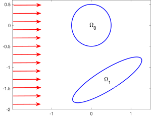
Figure 1: A multiple scattering configuration comprised of a circle $\Omega_{0}$ and an ellipse $\Omega_{1}$ illuminated by a plane wave incidence coming in from the left.

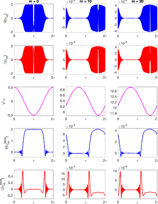
Figure 2: The real $\Re(\eta_{m})$ and imaginary $\Im(\eta_{m})$ parts of $\eta_{m}$ (first and second rows), the phase function $\phi_{m}$ (third row), and the real $\Re(\eta_{m}^{\rm slow})$ and imaginary $\Im(\eta_{m}^{\rm slow})$ parts of $\eta_{m}^{\rm slow}$ (fourth and fifth rows) for the wavenumber $k=800$ and reflections $m=0$ (left pane), $m=10$ (middle pane), and $m=20$ (right pane).

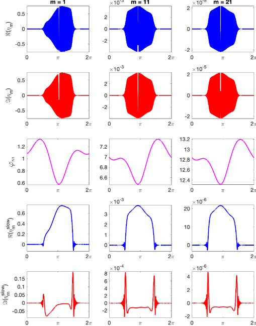
Figure 3: The real $\Re(\eta_{m})$ and imaginary $\Im(\eta_{m})$ parts of $\eta_{m}$ (first and second rows), the phase function $\phi_{m}$ (third row), and the real $\Re(\eta_{m}^{\rm slow})$ and imaginary $\Im(\eta_{m}^{\rm slow})$ parts of $\eta_{m}^{\rm slow}$ (fourth and fifth rows) for the wavenumber $k=800$ and reflections $m=1$ (left pane), $m=11$ (middle pane), and $m=21$ (right pane).

To validate Theorem 3 through numerical simulations, we consider a multiple scattering configuration consisting of two smooth strictly convex scatterers illuminated by a plane wave incidence coming in from the left ($\alpha=(1,0)$) as depicted in Fig. 1. The first obstacle there, denoted as $\Omega_{0}$, is a circle of radius $\frac{1}{2}$ centered at the origin and is taken with the parameterization $x(t)=\frac{1}{2}\left(\cos t,\sin t\right)$ ($0\leq t<2\pi$). The second scatterer, denoted as $\Omega_{1}$, is an ellipse $x(t)=\left(\frac{1}{4}\cos t,\sin t\right)$ ($0\leq t<2\pi$) rotated by $60^{\circ}$ in the clockwise direction and translated by the vector $\frac{1}{10}\left(4,-13\right)$. To illustrate Theorem 3, we consider the iterative solution of integral equations (19) for the wavenumber $k=800$ on the sequence of obstacles $\{K_{m}\}_{m\geq 0}$ where $K_{2m}=\Omega_{0}$ and $K_{2m+1}=\Omega_{1}$ so that $\eta_{m}$ is the total field generated on the circle $\Omega_{0}$ (respectively the ellipse $\Omega_{1}$) at the $m$-th iteration when $m$ is even (respectively odd).

Concerning the circle $\Omega_{0}$, in Fig. 2, we display the graphs of the real and imaginary parts of $\eta_{m}$, the phase function $\phi_{m}$, and the real and imaginary parts of $\eta_{m}^{\rm slow}$ (cf. (26)) at iterations $m=0$, $m=10$, and $m=20$. Similarly, in Fig. 3 we display the same data corresponding to the ellipse $\Omega_{1}$ at iterations $m=1$, $m=11$, and $m=21$.

The simulations depicted in Figures 2 and  3 are in agreement with the asymptotic expansions of the envelops $\eta_{m}^{\rm slow}$ presented in Theorem 3 as they support that $\eta_{m}^{\rm slow}$ admits a classical asymptotic expansion (cf. Theorem 3(i)) in the illuminated region $\partial K_{m}^{\rm IL}$ (27). This behavior transforms through a change in its asymptotic behavior (cf. Theorem 3(ii)) across the shadow boundaries $\partial K_{m}^{\rm SB}$ (28) to rapid decrease (cf. Theorem 3(iii)—but with additional oscillations not captured by the phase extraction) as one moves deep into the shadow region $\partial K_{m}^{\rm SR}$ (29).

6 Conclusions

In this paper, we derived the asymptotic expansions of the solutions of multiple scattering problem with the Neumann boundary condition. These expansions allowed for the derivation of sharp wavenumber dependent estimates related to their derivatives, more generally on the derivatives of envelopes obtained by subtracting finitely many terms in their asymptotic expansions as presented in Theorem 6. These estimates, in turn, can be used to extend the Galerkin boundary element methods for sound hard single scattering problems to multiple scattering scenarios for frequency independent implementations.

References

• [1] Milton Abramowitz and Irene A. Stegun. Handbook of mathematical functions with formulas, graphs, and mathematical tables, volume 55 of National Bureau of Standards Applied Mathematics Series. For sale by the Superintendent of Documents, U.S. Government Printing Office, Washington, D.C., 1964.
• [2] Akash Anand, Yassine Boubendir, Fatih Ecevit, and Fernando Reitich. Analysis of multiple scattering iterations for high-frequency scattering problems. II. The three-dimensional scalar case. Numer. Math., 114(3):373–427, 2010.
• [3] S. Arden, S. N. Chandler-Wilde, and S. Langdon. A collocation method for high-frequency scattering by convex polygons. J. Comput. Appl. Math., 204(2):334–343, 2007.
• [4] V. M. Babič and V. S. Buldyrev. Short-wavelength diffraction theory, volume 4 of Springer Series on Wave Phenomena. Springer-Verlag, Berlin, 1991. Asymptotic methods, Translated from the 1972 Russian original by E. F. Kuester.
• [5] Lehel Banjai and Wolfgang Hackbusch. Hierarchical matrix techniques for low- and high-frequency Helmholtz problems. IMA J. Numer. Anal., 28(1):46–79, 2008.
• [6] Steffen Börm. Efficient numerical methods for non-local operators, volume 14 of EMS Tracts in Mathematics. European Mathematical Society (EMS), Zürich, 2010. $H^{2}$-matrix compression, algorithms and analysis.
• [7] V. A. Borovikov and B. Ye. Kinber. Geometrical theory of diffraction, volume 37 of IEE Electromagnetic Waves Series. Institution of Electrical Engineers (IEE), London, 1994. Translated and revised from the Russian original.
• [8] Yassine Boubendir, Fatih Ecevit, and Fernando Reitich. Acceleration of an iterative method for the evaluation of high-frequency multiple scattering effects. SIAM J. Sci. Comput., 39(6):B1130–B1155, 2017.
• [9] Oscar Bruno, Christophe Geuzaine, and Fernando Reitich. On the $O(1)$ solution of multiple-scattering problems. IEEE Trans. Magn., 41(5):1488–1491, May 2005.
• [10] S. N. Chandler-Wilde, D. P. Hewett, S. Langdon, and A. Twigger. A high frequency boundary element method for scattering by a class of nonconvex obstacles. Numer. Math., 129(4):647–689, 2015.
• [11] S. N. Chandler-Wilde and S. Langdon. A Galerkin boundary element method for high frequency scattering by convex polygons. SIAM J. Numer. Anal., 45(2):610–640, 2007.
• [12] S. N. Chandler-Wilde and S. Langdon. Acoustic scattering: high-frequency boundary element methods and unified transform methods. In Unified transform for boundary value problems, pages 181–226. SIAM, Philadelphia, PA, 2015.
• [13] S. N. Chandler-Wilde, S. Langdon, and M. Mokgolele. A high frequency boundary element method for scattering by convex polygons with impedance boundary conditions. Commun. Comput. Phys., 11(2):573–593, 2012.
• [14] S. N. Chandler-Wilde, S. Langdon, and L. Ritter. A high-wavenumber boundary-element method for an acoustic scattering problem. Philos. Trans. R. Soc. Lond. Ser. A Math. Phys. Eng. Sci., 362(1816):647–671, 2004.
• [15] Simon N. Chandler-Wilde and Ivan G. Graham. Boundary integral methods in high frequency scattering. In Highly oscillatory problems, volume 366 of London Math. Soc. Lecture Note Ser., pages 154–193. Cambridge Univ. Press, Cambridge, 2009.
• [16] Simon N. Chandler-Wilde, Ivan G. Graham, Stephen Langdon, and Euan A. Spence. Numerical-asymptotic boundary integral methods in high-frequency acoustic scattering. Acta Numer., 21:89–305, 2012.
• [17] Eric T. Chung, Chi Yeung Lam, and Jianliang Qian. A ray-based IPDG method for high-frequency time-domain acoustic wave propagation in inhomogeneous media. J. Comput. Phys., 348:660–682, 2017.
• [18] David Colton and Rainer Kress. Inverse acoustic and electromagnetic scattering theory, volume 93 of Applied Mathematical Sciences. Springer-Verlag, Berlin, 1992.
• [19] David Colton and Rainer Kress. Integral equation methods in scattering theory, volume 72 of Classics Appl. Math. Philadelphia, PA: Society for Industrial and Applied Mathematics (SIAM), reprint of the 1983 original published by Wiley edition, 2013.
• [20] G. M. Constantine and T. H. Savits. A multivariate Faa di Bruno formula with applications. Trans. Amer. Math. Soc., 348:503–520, 1996.
• [21] V. Domínguez, I. G. Graham, and V. P. Smyshlyaev. A hybrid numerical-asymptotic boundary integral method for high-frequency acoustic scattering. Numer. Math., 106(3):471–510, 2007.
• [22] Fatih Ecevit. Frequency independent solvability of surface scattering problems. Turkish J. Math., 42(2):407–422, 2018.
• [23] Fatih Ecevit, Akash Anand, and Yassine Boubendir. Galerkin boundary element methods for high-frequency multiple-scattering problems. J. Sci. Comput., 83(1):Paper No. 1, 21, 2020.
• [24] Fatih Ecevit, Yassine Boubendir, Akash Anand, and Souaad Lazergui. Spectral Galerkin boundary element methods for high-frequency sound-hard scattering problems. Numer. Math., 150(3):803–847, 2022.
• [25] Fatih Ecevit and Hasan Hüseyin Eruslu. A Galerkin BEM for high-frequency scattering problems based on frequency-dependent changes of variables. IMA J. Numer. Anal., 39(2):893–923, 02 2019.
• [26] Fatih Ecevit and Hasan Çağan Özen. Frequency-adapted galerkin boundary element methods for convex scattering problems. Numer. Math., 135(1):27–71, 2017.
• [27] Fatih Ecevit and Fernando Reitich. Analysis of multiple scattering iterations for high-frequency scattering problems. I. The two-dimensional case. Numer. Math., 114(2):271–354, 2009.
• [28] Alexandre Ern and Jean-Luc Guermond. Finite elements, volume 72, 73, 74 of Texts in Applied Mathematics. Springer, Cham, 2021.
• [29] M. V. Fedoryuk. The stationary phase method and pseudodifferential operators. Russ. Math. Surv., 26(1):65, 1971.
• [30] Jeffrey Galkowski. Distribution of resonances in scattering by thin barriers. Mem. Amer. Math. Soc., 259(1248):ix+152, 2019.
• [31] Jeffrey Galkowski, Eike H. Müller, and Euan A. Spence. Wavenumber-explicit analysis for the Helmholtz $h$-BEM: error estimates and iteration counts for the Dirichlet problem. Numer. Math., 142(2):329–357, 2019.
• [32] A. Gibbs, D. P. Hewett, D. Huybrechs, and E. Parolin. Fast hybrid numerical-asymptotic boundary element methods for high frequency screen and aperture problems based on least-squares collocation. Partial Differ. Equ. Appl., 1(4):Paper No. 21, 26, 2020.
• [33] Andrew Gibbs, Simon N. Chandler-Wilde, Stephen Langdon, and Andrea Moiola. A high-frequency boundary element method for scattering by a class of multiple obstacles. IMA J. Numer. Anal., 41(2):1197–1239, 2021.
• [34] Walton C. Gibson. The method of moments in electromagnetics. CRC Press, Boca Raton, FL, second edition, 2015.
• [35] I. S. Gradshteyn and I. M. Ryzhik. Table of Integrals, Series, and Products. Academic Press Inc., San Diego, CA, 6th edition, 2000.
• [36] Samuel P. Groth, David P. Hewett, and Stephen Langdon. Hybrid numerical-asymptotic approximation for high-frequency scattering by penetrable convex polygons. IMA J. Appl. Math., 80(2):324–353, 2015.
• [37] S.P. Groth, D.P. Hewett, and S. Langdon. A hybrid numerical–asymptotic boundary element method for high frequency scattering by penetrable convex polygons. Wave Motion, 78:32–53, 2018.
• [38] D. P. Hewett, S. Langdon, and S. N. Chandler-Wilde. A frequency-independent boundary element method for scattering by two-dimensional screens and apertures. IMA J. Numer. Anal., 35(4):1698–1728, 2015.
• [39] D. P. Hewett, S. Langdon, and J. M. Melenk. A high frequency $hp$ boundary element method for scattering by convex polygons. SIAM J. Numer. Anal., 51(1):629–653, 2013.
• [40] Lars Hörmander. Pseudo-differential operators and hypoelliptic equations. Proc. Symp. Pure Math. 10, 138-183 (1967).
• [41] Lars Hörmander. Fourier integral operators. I. Acta Math., 127:79–183, 1971.
• [42] Jianming Jin. The finite element method in electromagnetics. Wiley-Interscience [John Wiley & Sons], New York, second edition, 2002.
• [43] Warren P. Johnson. The curious history of Faà di Bruno’s formula. Amer. Math. Monthly, 109(3):217–234, 2002.
• [44] Boško S. Jovanović and Endre Süli. Analysis of finite difference schemes, volume 46 of Springer Series in Computational Mathematics. Springer, London, 2014. For linear partial differential equations with generalized solutions.
• [45] Joseph B. Keller. Geometrical theory of diffraction. J. Opt. Soc. Amer., 52:116–130, 1962.
• [46] Joseph B. Keller and Robert M. Lewis. Asymptotic Methods for Partial Differential Equations: The Reduced Wave Equation and Maxwell’s Equations, pages 1–82. Springer US, Boston, MA, 1995.
• [47] Morris Kline and Irvin W. Kay. Electromagnetic theory and geometrical optics. Pure and Applied Mathematics, Vol. XII. Interscience Publishers John Wiley & Sons, Inc., New York-London-Sydney, 1965.
• [48] Chi Yeung Lam and Jianliang Qian. Numerical microlocal analysis by fast Gaussian wave packet transforms and application to high-frequency Helmholtz problems. SIAM J. Sci. Comput., 41(5):A2717–A2746, 2019.
• [49] S. Langdon and S. N. Chandler-Wilde. A wavenumber independent boundary element method for an acoustic scattering problem. SIAM J. Numer. Anal., 43(6):2450–2477, 2006.
• [50] Souaad Lazergui and Yassine Boubendir. Asymptotic expansions of the Helmholtz equation solutions using approximations of the Dirichlet to Neumann operator. J. Math. Anal. Appl., 456(2):767–786, 2017.
• [51] Randall J. LeVeque. Finite volume methods for hyperbolic problems. Cambridge Texts in Applied Mathematics. Cambridge University Press, Cambridge, 2002.
• [52] Randall J. LeVeque. Finite difference methods for ordinary and partial differential equations. Society for Industrial and Applied Mathematics (SIAM), Philadelphia, PA, 2007. Steady-state and time-dependent problems.
• [53] Robert M. Lewis. Asymptotic theory of wave-propagation. Arch. Rational Mech. Anal., 20:191–250, 1965.
• [54] Yijun Liu. Fast multipole boundary element method. Cambridge University Press, Cambridge, 2009. Theory and applications in engineering.
• [55] D. A. McNamara, C. W. I. Pistorius, and J. A. G. Malherbe. Introduction to the uniform geometrical theory of diffraction. The Artech House Antennas and Propagation Library. Artech House, Inc., Boston, MA, 1990.
• [56] Richard B. Melrose and Michael E. Taylor. Near peak scattering and the corrected Kirchhoff approximation for a convex obstacle. Adv. in Math., 55(3):242–315, 1985.
• [57] Jean-Claude Nédélec. Acoustic and electromagnetic equations, volume 144 of Applied Mathematical Sciences. Springer-Verlag, New York, 2001. Integral representations for harmonic problems.
• [58] N. C. Nguyen, J. Peraire, F. Reitich, and B. Cockburn. A phase-based hybridizable discontinuous Galerkin method for the numerical solution of the Helmholtz equation. J. Comput. Phys., 290:318–335, 2015.
• [59] Olof Runborg. Mathematical models and numerical methods for high frequency waves. Commun. Comput. Phys., 2(5):827–880, 2007.
• [60] Daniel Seibel. Boundary element methods for the wave equation based on hierarchical matrices and adaptive cross approximation. Numer. Math., 150(2):629–670, 2022.
• [61] Euan A. Spence, Ilia V. Kamotski, and Valery P. Smyshlyaev. Coercivity of combined boundary integral equations in high-frequency scattering. Comm. Pure Appl. Math., 68(9):1587–1639, 2015.
• [62] Jiguang Sun and Aihui Zhou. Finite element methods for eigenvalue problems. Monographs and Research Notes in Mathematics. CRC Press, Boca Raton, FL, 2017.
• [63] R. H. Tew, S. J. Chapman, J. R. King, J. R. Ockendon, and I. Zafarullah. Scalar wave diffraction by tangent rays. Wave Motion, 32(4):363–380, 2000.