Covert Beamforming Design for Integrated Radar Sensing and Communication Systems

Abstract

We propose covert beamforming design frameworks for integrated radar sensing and communication (IRSC) systems, where the radar can covertly communicate with legitimate users under the cover of the probing waveforms without being detected by the eavesdropper. Specifically, by jointly designing the target detection beamformer and communication beamformer, we aim to maximize the radar detection mutual information (MI) (or the communication rate) subject to the covert constraint, the communication rate constraint (or the radar detection MI constraint), and the total power constraint. For the perfect eavesdropper’s channel state information (CSI) scenario, we transform the covert beamforming design problems into a series of convex subproblems, by exploiting semidefinite relaxation, which can be solved via the bisection search method. Considering the high complexity of iterative optimization, we further propose a single-iterative covert beamformer design scheme based on the zero-forcing criterion. For the imperfect eavesdropper’s CSI scenario, we develop a relaxation and restriction method to tackle the robust covert beamforming design problems. Simulation results demonstrate the effectiveness of the proposed covert beamforming schemes for perfect and imperfect CSI scenarios.

I Introduction

Compared with the separated radar and communication systems, the integrated radar sensing and communication (IRSC) systems enjoy a smaller platform payload and power consumption [1], which holds great potential for both civilian and military applications, such as 5G vehicular network [2, 3], Wi-Fi based indoor positioning [4], and the advanced multi-function radio frequency concept (AMRFC)[5]. A critical challenge of developing IRSC systems is to design integrated waveforms that can realize detection and communication simultaneously to alleviate spectrum scarcity. To this end, various studies in the literature focused on the design of dual-functional waveforms[6, 7, 8, 9, 10]. Due to the inherent IRSC nature of openness and broadcasting, the critical information embedded in the waveform is susceptible to be intercepted and eavesdropped by the malicious users[11, 12].

The security and the covertness of the radar waveforms is crucial in radar system design. Although there is extensive literature on optimizing wireless communications and radar sensing simultaneously, the information security of IRSC lacks in-depth research so far. Recently, some works [11, 13, 12, 14, 15] have studied the secrecy of IRSC systems in terms of the physical layer security, which focuses on preventing the communication signal from being decoded by the adversary users. Specifically, in [11], the authors proposed three transmit beam pattern methods for maximizing the secrecy rate, the signal-to-interference and noise ratio (SINR), and minimizing transmit power, respectively. In [12], in order to reduce the risk of information security, a unified passive radar and communication system was proposed, which maximizes the signal interference-to-noise ratio (SINR) of the radar receiver under the condition that the information confidentiality rate is higher than a certain threshold. In [13], a novel framework was proposed for the transmit beamforming of the joint RadCom system, where the beamforming schemes are designed to formulate an appropriate radar beampattern, while guaranteeing the SINR and power budget of the communication applications. In [14], the artificial noise (AN) was utilized to minimize the signal-to-noise ratio (SNR) of radar targets subject to the legitimate users’ SINR constraint, where the target was regarded as a potential eavesdropper. In [15], an AN-aided secure beamforming design algorithm was developed to minimize the maximum eavesdropping SINR of the target, subject to the communication QoS requirements, the constant-modulus power and the beampattern similarity constraints. Although physical layer security technologies can protect information content from wiretapping, the communication behavior itself can expose sensitive information [16, 17, 18].

Different from physical layer security technologies, covert communication can guarantee a low probability of intercept by shielding the communication behaviors from potential wardens [19, 20, 21, 22, 23]. To conceal the transmission from the detection by the malicious eavesdropper, one of the feasible ways is to cover up the communication signal with the radar signal. In [24, 25], the authors first hide the communication symbol by utilizing the multi-path effects of tag/transponder (simply denoted as the ”tag”). Specifically, by using tags to modulate the reflection of the incident radar waveform into communication waveforms, the modulated communication waveform is embedded into the ambient radar pulse scattering, which acts as masking interference to maintain a low intercept probability. Note that, the covert communications in [24, 25] depend on extra environmental conditions (the multi-path effects of tags), which may not always be available in practice.

So far, covert communication for IRSC systems has not been well investigated. Particularly, the covert design framework for the IRSC systems has not been rigorously established. Against this background, this paper establishes a covert communication optimization framework for IRSC systems. To be specific, under the covert constraint, we propose two covert beamforming optimization frameworks for mutual information and covert rate maximization. The frameworks consider both the cases of perfect and imperfect channel state information. The main contributions of this work are summarized follows:

• Considering Willie’s (eavesdropper) channel state information (WCSI) being available at the radar, both the radar detection mutual information (MI) maximization and covert rate maximization are studied under both the covert and total transmit power constraint, which are non-convex and hard to solve. Based on semidefinite relaxation (SDR), we first relax the covert beamforming design optimization problem into a series of convex subproblems, and then efficiently solved them via the bisection search method.

• In order to avoid the high complexity of iterative optimization, we further propose a single-iterative covert beamformer design scheme based on the zero-forcing criterion. Specifically, by designing the target detection beamformer as a cover, we optimize the communication beamformer to be orthogonal to the WCSI, and thus the communication signals are projected onto the null space of Willie’s channel, and achieve covert communications.

• Furthermore, with imperfect WCSI, we develop a relaxation and restriction method to tackle the robust covert beamforming design optimization problems. Specifically, by exploiting the piecewise monotonicity property of the covert function, we first transform the covert constraint into a simplified and equivalent form facilitating robust beamforming design. Then, we relax the robust covert beamforming design optimization problems based on SDR, and restrict it into a convex semidefinite program (SDP). Extensive numerical results quantify the effects of the key design parameters on the system performance.

The remaining part of this paper is organized as follows. In Section II, we describe the IRSC system model and problem formulation. Then, we present our covert beamforming design with perfect WCSI in Section III. In Section IV, the robust covert beamforming design is developed for imperfect WCSI. Section V presents numerical results of the proposed covert beamforming design frameworks, and conclusions are drawn in Section VI. Table I presents the means of the key notations in this paper.

TABLE I: Summary of Key Notations

Notation	Description
$\rm{s_{\rm{R}}}$	Detection signal
$\rm{s_{\rm{C}}}$	Communication signal
${{\bf{h}}_{\rm{T}}}$	Channel gain vector of radar-target path
${{\bf{h}}_{\rm{B}}}$	Channel gain vector of radar-Bob path
${{\bf{h}}_{\rm{W}}}$	Channel gain vector of radar-Willie path
${{\bf{w}}_{\rm{R,0}}}$	Beamformer for ${s_{\rm{R}}}$
${{\bf{w}}_{\rm{R,1}}}$	Beamformer for $\rm{s_{\rm{R}}}$
${{\cal H}_{0}}$	The null hypothesis that the radar only sends $\rm{s_{\rm{R}}}$
${{\cal H}_{1}}$	The hypothesis that the radar sends both $\rm{s_{\rm{R}}}$ and $\rm{s_{\rm{C}}}$
${y_{\rm{W}}}$	Received signal of Willie
${p_{0}}\left({{y_{\rm{W}}}}\right)$	Likelihood function of ${{y_{\rm{W}}}}$ under ${{\cal H}_{0}}$
${p_{1}}\left({{y_{\rm{W}}}}\right)$	Likelihood function of ${{y_{\rm{W}}}}$ under ${{\cal H}_{1}}$
$D\left({{p_{1}}\left\|{{p_{0}}}\right.}\right)$	Kullback-Leibler (KL) divergence from $p_{1}(y_{\rm{W}})$ to $p_{0}(y_{\rm{W}})$
$\xi$	Total detection error probability
$P\left({{{\cal D}_{1}}\left|{{{\cal H}_{0}}}\right.}\right)$	False alarm (FA) probability
$P\left({{{\cal D}_{0}}\left|{{{\cal H}_{1}}}\right.}\right)$	Missed detection (MD) probability

II System Model and Problem Formulation

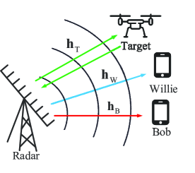
Figure 1:  The schematic diagram of a integrated radar-communication system.

Considering an integrated radar-communication system, as shown in Fig. 1, which includes a radar, a target, and a legitimate receiver (Bob). The radar with ${N}$ antennas is capable of detecting target and transmitting signals to the Bob simultaneously. While Bob is installed with a single antenna, and thus the reflected signals from the target can be ignored at Bob. In addition, an eavesdropper (Willie) with a single antenna keeps detecting the communication signals between the radar and Bob, and tries to identify whether the radar is transmitting information to Bob. Moreover, ${{\bf{h}}_{\rm{T}}}\in{\mathbb{C}^{N\times 1}}$, ${{\bf{h}}_{\rm{B}}}\in{\mathbb{C}^{N\times 1}}$ and ${{\bf{h}}_{\rm{W}}}\in{\mathbb{C}^{N\times 1}}$ denote channel state information (CSI) of the Radar-Target path, the Radar-Bob path and the Radar-Willie path, respectively. All channels are assumed followed the Rayleigh flat fading model [26], i.e., ${{\bf{h}}_{{\rm{B}}}}\sim\;{\cal C}{\cal N}\left({{\bf{0}},\sigma_{{\rm{1}}}^{\rm{2}}{\bf{I}}}\right),{{\bf{h}}_{{\rm{W}}}}\sim\;{\cal C}{\cal N}\left({{\bf{0}},\sigma_{{\rm{2}}}^{2}{\bf{I}}}\right)$, where $\sigma_{{\rm{1}}}^{2}$ and $\sigma_{{\rm{2}}}^{2}$ denote the variances of channels ${{\bf{h}}_{{\rm{T}}}}$, ${{\bf{h}}_{{\rm{B}}}}$, and ${{\bf{h}}_{{\rm{W}}}}$, respectively. Let $\rm{s_{\rm{R}}}$ and $\rm{s_{\rm{C}}}$ respectively denote the detection signal and and the communication signal of the radar . Without loss of generality, we assume that ${{\mathbb{E}}}\left\{{{{\left|{{s_{\rm{R}}}}\right|}^{2}}}\right\}=1$, ${{\mathbb{E}}}\left\{{{{\left|{{s_{\rm{C}}}}\right|}^{2}}}\right\}=1$.

II-A Signal Model

II-A1 Detection Only

The Radar-Target path ${\bf h}_{\rm{T}}$ can be expressed as

$${{\bf{h}}_{\rm{T}}}\triangleq{{\bf{a}}_{T}}(\theta),$$ (1)

where $\theta$ represents the azimuth angle of the target, and ${{\bf{a}}_{T}}(\theta)$ represents the transmit steering vector. Meanwhile, assume that $\mathbf{a}_{T}(\theta)\triangleq\mathbf{a}_{R}(\theta)$, where ${{\bf{a}}_{R}}(\theta)$ represents the receive steering vector [27]. Therefore, when the radar sends only detection signals and not the communication signals, the reflected signals from the target can be written as

$${{\bf{y}}_{\rm{R}}}=\alpha{{\bf{h}}_{\rm{T}}}{\bf{h}}_{\rm{T}}^{H}{{\bf{w}}_{{\rm{R}},{\rm{0}}}}{s_{\rm{R}}}+{{\bf{z}}_{\rm{R}}},$$ (2)

where $\alpha$ denotes the path-loss coefficient, ${{\bf{w}}_{\rm{R,0}}}$ denotes the radar transmission beamformer vector for ${s_{\rm{R}}}$ when the radar only sends detection signals, and ${\bf{z}_{\rm{R}}}\sim{\cal CN}\left({{\rm{0}},\sigma_{\rm{R}}^{2}{\bf{I}}}\right)$ is the received noise at the radar.

Here, we rely on the following standard assumptions: parameters $\alpha$ and $\theta$ can be estimated from the received signal [28]. Since the transmitted signals can be omni-directional, the legitimate user Bob could receive the detection signals as well. For Bob, we have

$${y_{\rm{B}}}={\bf{h}}_{\rm{B}}^{H}{{\bf{w}}_{{\rm{R}},{\rm{0}}}}{s_{\rm{R}}}+{z_{\rm{B}}},$$ (3)

where ${z_{\rm{B}}}\sim{\cal CN}\left({{\rm{0}},\sigma_{\rm{B}}^{2}}\right)$ is the receiver noise of Bob.

II-A2 Detection and Communication

The communication signals from the radar are also omni-directional. Moreover, since the radar has multiple antennas, the reflected communication signals from the target can also be captured. Thus, when the detection and the communication functions are performed simultaneously, the received signal at the radar is

$${{\bf{y}}_{\rm{R}}}=\alpha{{\bf{h}}_{\rm{T}}}{\bf{h}}_{\rm{T}}^{H}{{\bf{w}}_{{\rm{R}},0}}{s_{\rm{R}}}+\alpha{{\bf{h}}_{\rm{T}}}{\bf{h}}_{\rm{T}}^{H}{{\bf{w}}_{{\rm{R}},{\rm{1}}}}{s_{\rm{C}}}+{{\bf{z}}_{\rm{R}}},$$ (4)

where ${{\bf{w}}_{\rm{R,1}}}$ denotes the beamformer vectors for ${s_{\rm{C}}}$ when the radar sends detection signals and communication signals. For the legitimate user Bob, the received signal can be written as

$${y_{\rm{B}}}={{\bf{h}}_{\rm{B}}^{H}{{\bf{w}}_{{\rm{R}},0}}{s_{\rm{R}}}+{\bf{h}}_{\rm{B}}^{H}{{\bf{w}}_{{\rm{R}},{\rm{1}}}}{s_{\rm{C}}}+{z_{\rm{B}}}}.$$ (5)

II-B Performance Metrics

The considered system requires several metrics to measure the performance, according to the operating mode.

II-B1 Detection Only

For radar, by receiving the echo from the target, the radar estimates the channel ${\bf{h}}_{\rm{T}}$ and identifies some unknown characteristics about the target. Such characteristics can be quantified by using a tool from information theory which uses the observation at the channel output and reduces the uncertainty of prior information via certain code design. This tool successfully defines the information transmission capability of the communication channel [29]. This idea can also be used for the radar transmission design [29, 30, 31].

Specifically, after receiving ${{\bf{y}}_{\rm{R}}}$, the priori uncertainty of the target decreases since there is some information about the target contained in ${\bf{h}}_{\rm{T}}$ [29]. Thus, we adopt the mutual information (MI) between ${\bf{h}}_{\rm{T}}$ and ${{\bf{y}}_{\rm{R}}}$ given the transmission signal ${s_{\rm{R}}}$, i.e., ${\rm{I}}\left({{{\bf{y}}_{\rm{R}}};{{\bf{h}}_{\rm{T}}}\left|{{s_{\rm{R}}}}\right.}\right){\rm{}}$, to characterize how much information the radar can learn from ${{\bf{y}}_{\rm{R}}}$, which is given as

$$\begin{split}{\rm{I}}\left({{{\bf{y}}_{\rm{R}}};{{\bf{h}}_{\rm{T}}}\left|{{s_{\rm{R}}}}\right.}\right){\rm{}}&=\frac{1}{2}\log\left({1+\frac{{{{\left|\alpha\right|}^{2}}{{\left|{{\bf{h}}_{\rm{T}}^{H}{{\bf{w}}_{{\rm{R}},{\rm{0}}}}}\right|}^{2}}{{\left\|{{{\bf{h}}_{\rm{T}}}}\right\|}^{2}}}}{{\sigma_{\rm{R}}^{2}}}}\right).\end{split}$$ (6)

II-B2 Detection and Communication

For the MI at the radar, according to $\eqref{part1_03_2}$, we have

$$\rm{I}\left({{{\bf{y}}_{\rm{R}}};{{\bf{h}}_{\rm{T}}}\left|{{s_{\rm{R}}}}\right.}\right) =h\left({{{\bf{y}}_{\rm{R}}}\left|{{s_{\rm{R}}}}\right.}\right)-h\left({{{\bf{y}}_{\rm{R}}}\left|{{{\bf{h}}_{\rm{T}}},{s_{\rm{R}}}}\right.}\right)$$

$$=\frac{1}{2}\log\left({1+\frac{{{{\left|\alpha\right|}^{2}}{{\left|{{\bf{h}}_{\rm{T}}^{H}{{\bf{w}}_{{\rm{R,0}}}}}\right|}^{2}}{{\left\|{{{\bf{h}}_{\rm{T}}}}\right\|}^{2}}}}{{{{\left|\alpha\right|}^{2}}{{\left|{{\bf{h}}_{\rm{T}}^{H}{{\bf{w}}_{{\rm{R,1}}}}}\right|}^{2}}{{\left\|{{{\bf{h}}_{\rm{T}}}}\right\|}^{2}}+\sigma_{{{\bf{z}}_{\rm{R}}}}^{2}}}}\right).$$

Thus, based on $\eqref{part1_01_2}$, the achievable rate of Bob can be expressed as [32]

$${R_{\rm{B}}}\left({{{\bf{w}}_{{\rm{R}},{\rm{0}}}},{{\bf{w}}_{{\rm{R}},{\rm{1}}}}}\right)={\log_{2}}\left({1+\frac{{{{\left|{{\bf{h}}_{\rm{B}}^{H}{{\bf{w}}_{{\rm{R,1}}}}}\right|}^{2}}}}{{{{\left|{{\bf{h}}_{\rm{B}}^{H}{{\bf{w}}_{{\rm{R,0}}}}}\right|}^{2}}+\sigma_{\rm{B}}^{2}}}}\right).$$ (8)

II-C Covert Constraints

In the considered system, the eavesdropper Willie aims to determine whether Bob is communicating with the radar. Mathematically, Willie needs to perform a hypothesis test between the two hypotheses from its received signal ${y_{\rm{W}}}$. Here, ${{\cal H}_{0}}$ represents the null hypothesis, i.e., the radar only sends detection signals; ${{\cal H}_{1}}$ represents the other hypothesis, where the radar sends detection signals and communication signals. Thus, ${y_{\rm{W}}}$ can be written as

$${y_{\rm{W}}}=\left\{{\begin{array}[]{*{20}{c}}{{\bf{h}}_{\rm{W}}^{H}{{\bf{w}}_{{\rm{R}},{\rm{0}}}}{s_{\rm{R}}}+{z_{\rm{W}}},}&{{{\cal H}_{0}}},\\ {{\bf{h}}_{\rm{W}}^{H}{{\bf{w}}_{{\rm{R}},0}}{s_{\rm{R}}}+{\bf{h}}_{\rm{W}}^{H}{{\bf{w}}_{{\rm{R,1}}}}{s_{\rm{C}}}+{z_{\rm{W}}},}&{{{\cal H}_{1}}},\end{array}}\right.$$ (11)

where ${z_{\rm{W}}}\sim{\cal CN}\left({{\rm{0}},\sigma_{\rm{W}}^{2}}\right)$ is the receiving noise at Willie. Note that, when the radar performs tracking and communication, the radar needs to assume the existence of Willie and tries to conceal the communication with Bob.

In the following, we will introduce the covert constraint to describe the level of covertness. Specifically, for Willie, let ${p_{0}}\left({{y_{\rm{W}}}}\right)$ and ${p_{1}}\left({{y_{\rm{W}}}}\right)$ to represent the likelihood function of ${{y_{\rm{W}}}}$ under ${{\cal H}_{0}}$ and ${{\cal H}_{1}}$, respectively. According to $\eqref{part1_02}$, ${p_{0}}\left({{y_{\rm{W}}}}\right)$ and ${p_{1}}\left({{y_{\rm{W}}}}\right)$ can be expressed as

$${p_{0}}\left({{y_{\rm{W}}}}\right)=\frac{1}{{\pi{\lambda_{0}}}}\exp\left({-\frac{{{{\left|{{y_{\rm{W}}}}\right|}^{2}}}}{{{\lambda_{0}}}}}\right),$$ (12a)

$${p_{1}}\left({{y_{\rm{W}}}}\right)=\frac{1}{{\pi{\lambda_{1}}}}\exp\left({-\frac{{{{\left|{{y_{\rm{W}}}}\right|}^{2}}}}{{{\lambda_{1}}}}}\right),$$ (12b)

where ${\lambda_{\rm{0}}}\buildrel\Delta\over{=}{\left|{{\bf{h}}_{\rm{W}}^{H}{{\bf{w}}_{\rm{R,0}}}}\right|^{2}}+\sigma_{\rm{W}}^{2}$ and ${\lambda_{\rm{1}}}\buildrel\Delta\over{=}{\left|{{\bf{h}}_{\rm{W}}^{H}{{\bf{w}}_{\rm{R,0}}}}\right|^{2}}+{\left|{{\bf{h}}_{{\rm{W}}}^{H}{{\bf{w}}_{\rm{R,1}}}}\right|^{2}}+\sigma_{\rm{W}}^{2}$. Moreover, let $D\left({{p_{0}}\left\|{{p_{1}}}\right.}\right)$ denote the KL divergence from $p_{0}(y_{\rm{W}})$ to $p_{1}(y_{\rm{W}})$, and $D\left({{p_{1}}\left\|{{p_{0}}}\right.}\right)$ denote the KL divergence from $p_{1}(y_{\rm{W}})$ to $p_{0}(y_{\rm{W}})$. According to $\eqref{part1_05}$, $D\left({{p_{0}}\left\|{{p_{1}}}\right.}\right)$ and $D\left({{p_{1}}\left\|{{p_{0}}}\right.}\right)$ are respectively given as

$$D\left({{p_{0}}\left\|{{p_{1}}}\right.}\right) =\int_{-\infty}^{+\infty}{{p_{0}}\left({{y_{\text{W}}}}\right)\ln\frac{{{p_{0}}\left({{y_{\text{W}}}}\right)}}{{{p_{1}}\left({{y_{\text{W}}}}\right)}}}dy=\ln\frac{{{\lambda_{1}}}}{{{\lambda_{0}}}}+\frac{{{\lambda_{0}}}}{{{\lambda_{1}}}}-1,$$ (13a)

$$D\left({{p_{1}}\left\|{{p_{0}}}\right.}\right) =\int_{-\infty}^{+\infty}{{p_{1}}\left({{y_{\text{W}}}}\right)\ln\frac{{{p_{1}}\left({{y_{\text{W}}}}\right)}}{{{p_{0}}\left({{y_{\text{W}}}}\right)}}}dy=\ln\frac{{{\lambda_{0}}}}{{{\lambda_{1}}}}+\frac{{{\lambda_{1}}}}{{{\lambda_{0}}}}-1.$$ (13b)

II-C1 Detection by Willie

Let ${{{\cal D}_{1}}}$ and ${{{\cal D}_{0}}}$ denote the binary decisions that correspond to hypotheses ${{{\cal H}_{0}}}$ and ${{{\cal H}_{1}}}$, respectively. The detecting performance at Willie is described by the FA probability $P\left({{{\cal D}_{1}}\left|{{{\cal H}_{0}}}\right.}\right)$ and the MD probability $P\left({{{\cal D}_{0}}\left|{{{\cal H}_{1}}}\right.}\right)$. The total detection error probability $\xi$ can be used to measure the covertness of the system [33], i.e.,

$$\xi=P\left({{{\cal D}_{1}}\left|{{{\cal H}_{0}}}\right.}\right)+P\left({{{\cal D}_{0}}\left|{{{\cal H}_{1}}}\right.}\right).$$ (14)

To further evaluate $\eqref{part1_09}$, we assume that the probabilities ${{\cal H}_{0}}$ and ${{\cal H}_{1}}$ are equal. By applying the Neyman-Pearson criterion [33], the optimal rule for Willie to minimize $\xi$ as the likelihood ratio test, i.e.,

$$\frac{{{p_{1}}\left({{y_{\rm{W}}}}\right)}}{{{p_{0}}\left({{y_{\rm{W}}}}\right)}}\frac{{\mathop{>}\limits^{{D_{1}}}}}{{\mathop{<}\limits_{{D_{0}}}}}1.$$ (15)

After some algebraic operations, $\eqref{C_17}$ can be equivalently reformulated as

$${\left|{{y_{\rm{W}}}}\right|^{2}}\frac{{\mathop{>}\limits^{{{\cal D}_{1}}}}}{{\mathop{<}\limits_{{{\cal D}_{0}}}}}{\phi^{*}},$$ (16)

where ${\left|{{y_{\rm{W}}}}\right|^{2}}$ is the average power at Willie, and $\phi^{*}$ denotes the optimal detection threshold of Willie, which is given by

$${\phi^{*}}\buildrel\Delta\over{=}\frac{{{\lambda_{0}}{\lambda_{1}}}}{{{\lambda_{1}}-{\lambda_{0}}}}{\rm{ln}}\frac{{{\lambda_{1}}}}{{{\lambda_{0}}}}.$$ (17)

According to $\eqref{part1_05}$, the cumulative density functions (CDFs) of ${\left|{{y_{\rm{W}}}}\right|^{2}}$ under ${{{\cal H}_{\rm{0}}}}$ and ${{{\cal H}_{\rm{1}}}}$ are given by

$$\Pr\left({\left.{{{\left|{{y_{\rm{W}}}}\right|}^{2}}}\right|{\cal{H}_{\rm{0}}}}\right)=1-\exp\left({-\frac{{{{\left|{{y_{\rm{W}}}}\right|}^{2}}}}{{{\lambda_{0}}}}}\right),$$ (18a)

$$\Pr\left({\left.{{{\left|{{y_{\rm{W}}}}\right|}^{2}}}\right|{\cal{H}_{\rm{1}}}}\right)=1-\exp\left({-\frac{{{{\left|{{y_{\rm{W}}}}\right|}^{2}}}}{{{\lambda_{1}}}}}\right).$$ (18b)

Based on the optimal detection threshold ${\phi^{*}}$, we obtain

$$P\left({{{\cal D}_{1}}\left|{{{\cal H}_{0}}}\right.}\right)={\Pr}\left({{{\left|{{y_{\rm{W}}}}\right|}^{2}}\geq{\phi^{*}}|{{{\cal H}_{\rm{0}}}}}\right)={\left({\frac{{{\lambda_{1}}}}{{{\lambda_{0}}}}}\right)^{-\frac{{{\lambda_{1}}}}{{{\lambda_{1}}-{\lambda_{0}}}}}},$$

$$P\left({{{\cal D}_{0}}\left|{{{\cal H}_{1}}}\right.}\right)={\Pr}\left({{{\left|{{y_{\rm{W}}}}\right|}^{2}}\leq{\phi^{*}}|{{{\cal H}_{\rm{1}}}}}\right)=1-{\left({\frac{{{\lambda_{1}}}}{{{\lambda_{0}}}}}\right)^{-\frac{{{\lambda_{0}}}}{{{\lambda_{1}}-{\lambda_{0}}}}}}.$$

II-C2 Definition of Covert Constraint

The eavesdropper Willie tries to find the best detector with the least total detection error probability $\xi^{*}$ [34]. From the legitimate user perspective, an effective covert communication should guarantee that no matter what strategy Willie adopts, for any given small constant $\varepsilon\in\left[{0,1}\right]$, the following criterion can be satisfied $\xi^{*}\geq 1-\varepsilon$[33]. Thus, when Willie adopts the optimal detector, we have [33, 34, 35, 36]

$$\xi^{*}=1-{V_{\rm{T}}}\left({{p_{0}},{p_{1}}}\right).$$ (20)

where ${V_{\rm{T}}}\left({{p_{0}},{p_{1}}}\right)$ is expressed as the total variation distance between ${p_{0}}$ and ${p_{1}}$.

Furthermore, based on Pinsker’s inequality [37], we obtain

$${V_{\rm{T}}}\left({{p_{0}},{p_{1}}}\right)\leq\sqrt{\frac{1}{2}D\left({{p_{0}}\left\|{{p_{1}}}\right.}\right)},$$ (21a)

$${V_{\rm{T}}}\left({{p_{0}},{p_{1}}}\right)\leq\sqrt{\frac{1}{2}D\left({{p_{1}}\left\|{{p_{0}}}\right.}\right)}.$$ (21b)

Therefore, by combining the formulas (20) and (21), we obtain the tractable covert constraints as follows

$$D\left({{p_{0}}\left\|{{p_{1}}}\right.}\right)\leq 2{\varepsilon^{2}},$$ (22a)

$$D\left({{p_{1}}\left\|{{p_{0}}}\right.}\right)\leq 2{\varepsilon^{2}}{{,}}$$ (22b)

which are determined by the transmission variables and the receiver noise (see $\eqref{part1_08}$).

II-D Problem Formulation

Given the two performance metrics when the radar performs the detection and communication at the same time, an intuitive optimization goal is to make these two metrics as large as possible. Thus, we obtain the following two terms optimization problems, i.e., the radar MI maximization problem and the communication rate maximization problem.

II-D1 MI Maximization

As described above, a larger MI indicates more possibilities to identify the information about the target from the received signals. Thus, we aim to design beamforming vectors with the maximum MI $\eqref{MI}$ while satisfying the covert constraint, the covert rate requirement and the total transmit power constraints, which can be mathematically formulated as

$$\mathop{\max}\limits_{{{\bf{w}}_{{\rm{R,0}}}},{{\bf{w}}_{{\rm{R,1}}}}} {\rm{I}}\left({{\bf{y}_{\rm{R}}};{{\bf{h}}_{\rm{T}}}\left|{{s_{\rm{R}}}}\right.}\right)$$ (23a)

$${\rm{s}}.{\rm{t}}.\quad {R_{\rm{B}}}\left({{{\bf{w}}_{{\rm{R}},{\rm{0}}}},{{\bf{w}}_{{\rm{R}},{\rm{1}}}}}\right)\geq\beta,$$ (23b)

$${\left\|{{{\bf{w}}_{{\rm{R}},{\rm{0}}}}}\right\|^{2}}+{\left\|{{{\bf{w}}_{{\rm{R}},{\rm{1}}}}}\right\|^{2}}\leq{P_{{\rm{total}}}},$$ (23c)

$$\eqref{part1_07_1}{\quad\rm{or}\quad}\eqref{part1_07_2},$$

where ${P_{{\rm{total}}}}$ denotes the maximum radar transmit power.

II-D2 Rate Maximization

The objective of this problem is to design a beamformer that maximizes the rate achieved by Bob while satisfying the required covertness constraints, the MI requirement, and the total transmit power constraints. Mathematically, the problem of maximizing the achievable rates can be expressed as

$$\mathop{\max}\limits_{{{\bf{w}}_{{\rm{R,0}}}},{{\bf{w}}_{{\rm{R,1}}}}} {R_{\rm{B}}}\left({{{\bf{w}}_{{\rm{R}},{\rm{0}}}},{{\bf{w}}_{{\rm{R}},{\rm{1}}}}}\right)$$ (24a)

$${\rm{s}}.{\rm{t}}.\quad {\rm{I}}\left({{\bf{y}_{\rm{R}}};{{\bf{h}}_{\rm{T}}}\left|{{s_{\rm{R}}}}\right.}\right)\geq\gamma,$$ (24b)

$${\left\|{{{\bf{w}}_{{\rm{R}},{\rm{0}}}}}\right\|^{2}}+{\left\|{{{\bf{w}}_{{\rm{R}},{\rm{1}}}}}\right\|^{2}}\leq{P_{{\rm{total}}}},$$ (24c)

$$\eqref{part1_07_1}{\quad\rm{or}\quad}\eqref{part1_07_2}.$$

Remarks: Note that, when the radar performs detection only, the corresponding optimization problem becomes a simplified version of problem $\eqref{C2}$. Thus, we omit this case, and only investigate the integrated radar sensing and communication case. From the above formulations, the two optimization problems (23) and (24) have similar structure. Basically, for the MI and the covert rate, the beamformer splits the available power to maximize one term while satisfying the requirement of the other term. Hence, there should exist a tradeoff between the MI and the covert rate. In the following, we will focus on the investigation of the MI maximization problem, and numerically discuss the tradeoff.

III Beamforming Design based on PERFECT WCSI

We first consider a typical scenario, where Willie is a legitimate user. In this case, the radar may obtain the full CSI of ${{\bf{h}}_{\rm{W}}}$, and uses it to help Bob to hide from Willie under ${{\cal H}_{1}}$ [35, 32]. Then, the covert constraint becomes

$$D\left({{p_{0}}\left\|{{p_{1}}}\right.}\right)=0,$$ (25a)

$$D\left({{p_{1}}\left\|{{p_{0}}}\right.}\right)=0.$$ (25b)

Note that, $\eqref{D}$ also implies the perfect covert transmission.

III-A MI Maximization

After applying formula $\eqref{C2}$, the MI maximization problem can be reformulated as

$$\mathop{\max}\limits_{{{\bf{w}}_{{\rm{R,0}}}},{{\bf{w}}_{{\rm{R,1}}}}} \frac{1}{2}\log\left({1+\frac{{{\left|\alpha\right|^{2}}{{\left|{{\bf{h}}_{\rm{T}}^{H}{{\bf{w}}_{{\rm{R,0}}}}}\right|}^{2}}{{\left\|{{{\bf{h}}_{\rm{T}}}}\right\|}^{2}}}}{{{\left|\alpha\right|^{2}}{{\left|{{\bf{h}}_{\rm{T}}^{H}{{\bf{w}}_{{\rm{R,1}}}}}\right|}^{2}}{{\left\|{{{\bf{h}}_{\rm{T}}}}\right\|}^{2}}+\sigma_{\rm{R}}^{2}}}}\right)$$ (26a)

$${\rm{s}}.{\rm{t}}.\quad {\left|{{\bf{h}}_{\rm{W}}^{H}{{\bf{w}}_{{\rm{R,1}}}}}\right|^{2}}=0,$$ (26b)

$$\frac{{{{\left|{{\bf{h}}_{\rm{B}}^{H}{{\bf{w}}_{{\rm{R,1}}}}}\right|}^{2}}}}{{{{\left|{{\bf{h}}_{\rm{B}}^{H}{{\bf{w}}_{{\rm{R,0}}}}}\right|}^{2}}+\sigma_{\rm{B}}^{2}}}\geq\beta,$$ (26c)

$${\left\|{{{\bf{w}}_{{\rm{R}},{\rm{0}}}}}\right\|^{2}}+{\left\|{{{\bf{w}}_{{\rm{R}},{\rm{1}}}}}\right\|^{2}}\leq{P_{{\rm{total}}}}.$$ (26d)

Next, we propose two different methods, namely covert beamformer and zero-forcing beamformer, to solve problem (26).

III-A1 Covert Beamformer

By introducing an auxiliary variable ${\rm{I}_{\rm{R}}}$, the above problem can be reformulated in the following equivalent form:

$$\mathop{\max}\limits_{{{\bf{w}}_{\rm{R,0}}},{{\bf{w}}_{{\rm{R,1}}}},{\rm{I}_{\rm{R}}}} {\rm{I}_{\rm{R}}}$$ (27a)

$${\rm{s}}.{\rm{t}}.\quad {\frac{{{{\left|\alpha\right|^{2}}{\left|{{\bf{h}}_{\rm{T}}^{H}{{\bf{w}}_{{\rm{R,0}}}}}\right|}^{2}{{\left\|{{{\bf{h}}_{\rm{T}}}}\right\|}^{2}}}}}{{{\left|\alpha\right|^{2}}{{\left|{{\bf{h}}_{\rm{T}}^{H}{{\bf{w}}_{{\rm{R,1}}}}}\right|}^{2}{{\left\|{{{\bf{h}}_{\rm{T}}}}\right\|}^{2}}}+\sigma_{\rm{R}}^{2}}}}\geq{\rm{I}_{\rm{R}}},$$ (27b)

$${\left|{{\bf{h}}_{\rm{W}}^{H}{{\bf{w}}_{{\rm{R,1}}}}}\right|^{2}}=0,$$ (27c)

$$\frac{{{{\left|{{\bf{h}}_{\rm{B}}^{H}{{\bf{w}}_{{\rm{R,1}}}}}\right|}^{2}}}}{{{{\left|{{\bf{h}}_{\rm{B}}^{H}{{\bf{w}}_{{\rm{R,0}}}}}\right|}^{2}}+\sigma_{\rm{B}}^{2}}}\geq\beta,$$ (27d)

$${\left\|{{{\bf{w}}_{{\rm{R}},{\rm{0}}}}}\right\|^{2}}+{\left\|{{{\bf{w}}_{{\rm{R}},{\rm{1}}}}}\right\|^{2}}\leq{P_{{\rm{total}}}}.{\rm{}}$$ (27e)

Then, we use the semidefinite relaxation (SDR) approach [38] to relax problem $\eqref{part22_03}$ to

$${{\bf{W}}_{\rm{R,0}}}={{\bf{w}}_{\rm{R,0}}}{\bf{w}}_{\rm{R,0}}^{H}\Leftrightarrow{{\bf{W}}_{\rm{R,0}}}\underline{\succ}{\bf{0}},{\rm{rank}}\left({{{\bf{W}}_{\rm{R,0}}}}\right)=1,$$ (28a)

$${{\bf{W}}_{{\rm{R,1}}}}={{\bf{w}}_{{\rm{R,1}}}}{\bf{w}}_{{\rm{R,1}}}^{H}\Leftrightarrow{{\bf{W}}_{{\rm{R,1}}}}\underline{\succ}{\bf{0}},{\rm{rank}}\left({{{\bf{W}}_{{\rm{R,1}}}}}\right)=1.$$ (28b)

By ignoring the rank 1 constraints, we get a relaxed version of problem $\eqref{part22_03}$ as follows

$$\mathop{\max}\limits_{{{\bf{w}}_{\rm{R,0}}},{{\bf{w}}_{{\rm{R,1}}}},{\rm{I}_{\rm{R}}}} {\rm{I}_{\rm{R}}}$$ (29)

$${\rm{s}}.{\rm{t}}.\quad {\left|\alpha\right|^{2}}{\rm{Tr}}\left({{\bf{h}}_{\rm{T}}^{H}{{\bf{W}}_{{\rm{R}},{\rm{0}}}}{{\bf{h}}_{\rm{T}}}}\right){\left\|{{{\bf{h}}_{\rm{T}}}}\right\|^{2}}\geq{{\rm{I}}_{\rm{R}}}\left({{{\left|\alpha\right|}^{2}}}\right.$$

$$\qquad\left.{\times{\rm{Tr}}\left({{\bf{h}}_{\rm{T}}^{H}{{\bf{W}}_{{\rm{R}},{\rm{1}}}}{{\bf{h}}_{\rm{T}}}}\right){{\left\|{{{\bf{h}}_{\rm{T}}}}\right\|}^{2}}+\sigma_{\rm{R}}^{2}}\right),$$

$${\rm{Tr}}\left({{\bf{h}}_{\rm{B}}^{H}{{\bf{W}}_{{\rm{R,1}}}}{{\bf{h}}_{\rm{B}}}}\right)\geq\beta\left({{\rm{Tr}}\left({{\bf{h}}_{\rm{B}}^{H}{{\bf{W}}_{{\rm{R,0}}}}{{\bf{h}}_{\rm{B}}}}\right)+\sigma_{\rm{B}}^{2}}\right),$$

$${\rm{Tr}}\left({{\bf{h}}_{\rm{W}}^{H}{{\bf{W}}_{{\rm{R,1}}}}{{\bf{h}}_{\rm{W}}}}\right)=0,$$

$${\rm{Tr}}\left({{{\bf{W}}_{{\rm{R}},{\rm{0}}}}}\right)+{\rm{Tr}}\left({{{\bf{W}}_{\rm{R,1}}}}\right)\leq{P_{{\rm{total}}}},$$

$${{\bf{W}}_{{\rm{R}},{\rm{0}}}}\underline{\succ}{\bf{0}},{{\bf{W}}_{\rm{R,1}}}\underline{\succ}{\bf{0}}.$$

Note that, for any ${\rm{I}_{\rm{R}}}\geq 0$, it is a convex semidefinite program (SDP). Therefore, it is quasi-convex, and at any given ${\rm{I}_{\rm{R}}}$, by testing its feasibility, the optimal solution can be found.

Therefore, we first covert problem $\eqref{part22_04}$ into a series of convex subproblems of ${\rm{I}_{\rm{R}}}\geq 0$, which can be solved by a standard convex optimization solver (such as CVX). Then, we use the bisection search method to find the proposed covert beamformers ${{\bf{W}}_{\rm{R,0}}}$ and ${{\bf{W}}_{\rm{R,1}}}$, which output the optimal solutions ${\bf{W}}_{\rm{R,0}}^{*}$ and ${\bf{W}}_{\rm{R,1}}^{*}$.

Algorithm 1 Bisection method for problem (29)

1:Determine the interval $\left[{{\rm{I}_{{\rm{R,l}}}},{\rm{I}_{{\rm{R,end}}}}}\right]$, given the accuracy $\zeta_{1}>0$;

2:Initialize ${\rm{I}_{{\rm{R,l}}}}=0$, ${\rm{I}_{{\rm{R,end}}}}={{\hat{\rm{I}}}_{\rm{R}}}$;

3:while ${{\rm{I}}_{{\rm{R,end}}}}-{{\rm{I}}_{{\rm{R,l}}}}\geq\zeta_{1}$ do

4:     set ${{\rm{I}}_{{\rm{R}}}}=\left({{{\rm{I}}_{{\rm{R,l}}}}+{{\rm{I}}_{{\rm{R,end}}}}}\right)/2$;

5:     if problem (29) is solvable, get ${{\bf{W}}_{\rm{R,0}}}$ and ${{\bf{W}}_{{\rm{R}},1}}$, then set ${{\rm{I}}_{{\rm{R,l}}}}={{\rm{I}}_{{\rm{R}}}}$;

6:     else, set ${{\rm{I}}_{{\rm{R,end}}}}={{\rm{I}}_{{\rm{R,mid}}}}$;

7:end while

8:Output ${\bf{W}}_{{\rm{R}},1}^{*}$,${\bf{W}}_{\rm{R,0}}^{*}$;

Finally, we can solve this problem based on the solutions given by Algorithm 1. The computational complexity of Algorithm 1 is ${\cal O}\left({\max{{\left\{{4,2N}\right\}}^{4}}\sqrt{2N}\log\left({{1\mathord{\left/{\vphantom{1{{\xi_{1}}}}}\right.\kern-1.2pt}{{\zeta_{1}}}}}\right)\log\left({{1\mathord{\left/{\vphantom{1\zeta_{1}}}\right.\kern-1.2pt}\zeta_{1}}}\right)}\right)$, where ${\zeta_{1}}>0$ is the pre-defined accuracy of problem (29) [38, 39, 40]. However, because of the rank relaxation of SDR, the ranks of the optimal solutions ${\bf{W}}_{\rm{R,0}}^{*}$ and ${\bf{W}}_{\rm{R,1}}^{*}$ may larger than 1. When ${\rm{rank}}\left({{\bf{W}}_{\rm{R,0}}^{*}}\right)=1$ and ${\rm{rank}}\left({{\bf{W}}_{\rm{R,1}}^{*}}\right)=1$, we employ the singular value decomposition to decompose ${\bf{W}}_{\rm{R,0}}^{*}$ and ${\bf{W}}_{\rm{R,1}}^{*}$, i.e., ${{\bf{W}}_{\rm{R,0}}}={{\bf{w}}_{\rm{R,0}}}{\bf{w}}_{\rm{R,0}}^{H}$ and ${{\bf{W}}_{{\rm{R,1}}}}={{\bf{w}}_{{\rm{R,1}}}}{\bf{w}}_{{\rm{R,1}}}^{H}$. On the other hand, when ${\rm{rank}}\left({{\bf{W}}_{\rm{R,0}}^{*}}\right)>1$ or ${\rm{rank}}\left({{\bf{W}}_{\rm{R,1}}^{*}}\right)>1$, we apply the Gaussian randomization procedure [38] to problem $\eqref{part22_03}$ and get high-quality rank $1$ beamformers.

III-A2 Zero-Forcing Beamformer

To eliminate interference signals of Willie and the radar, we design zero-forcing beamformer ${{\bf{w}}_{\rm{R,1}}}$ satisfying ${\bf{h}}_{{\rm{W}}}^{H}{{\bf{w}}_{\rm{R,1}}}=0$ and ${\bf{h}}_{\rm{T}}{\bf{h}}_{{\rm{T}}}^{H}{{\bf{w}}_{\rm{R,1}}}=\bf{0}$. In addition, we design ${{\bf{w}}_{{\rm{R,0}}}}$ to eliminate Bob’s interference, i.e., ${\bf{h}}_{{\rm{B}}}^{H}{{\bf{w}}_{{\rm{R,0}}}}=0$. Then, problem $\eqref{part22_02}$ can be expressed as

$$\mathop{\max}\limits_{{{\bf{w}}_{{\rm{R}},{\rm{0}}}},{{\bf{w}}_{{\rm{R}},{\rm{1}}}}} {\left|{{\bf{h}}_{\rm{T}}^{H}{{\bf{w}}_{{\rm{R}},0}}}\right|^{2}}$$ (30a)

$${\rm{s}}{\rm{.t}}{\rm{.}}\quad {\bf{h}}_{\rm{T}}^{H}{{\bf{w}}_{{\rm{R}},{\rm{1}}}}=0,$$ (30b)

$${\bf{h}}_{\rm{W}}^{H}{{\bf{w}}_{{\rm{R}},{\rm{1}}}}=0,$$ (30c)

$${\bf{h}}_{{\rm{B}}}^{H}{{\bf{w}}_{{\rm{R,0}}}}=0,$$ (30d)

$${\left|{{\bf{h}}_{\rm{B}}^{H}{{\bf{w}}_{{\rm{R}},{\rm{1}}}}}\right|^{2}}\geq\beta\sigma_{\rm{B}}^{\rm{2}},$$ (30e)

$${\left\|{{{\bf{w}}_{{\rm{R}},{\rm{0}}}}}\right\|^{2}}+{\left\|{{{\bf{w}}_{\rm{R,1}}}}\right\|^{2}}\leq{P_{{\rm{total}}}}.$$ (30f)

To solve problem (30), we first optimize the beamformer ${{{\bf{w}}_{{\rm{R}},{\rm{1}}}}}$ by minimizing the transmission power ${\left\|{{{\bf{w}}_{{\rm{R}},{\rm{1}}}}}\right\|^{2}}$ under the constraints $\eqref{part22_11_2}$, $\eqref{part22_11_3}$ and $\eqref{part22_11_7}$. This is because the value of the objective function $\eqref{part22_11_1}$ increases as the power of ${{\bf{w}}_{\rm{R,0}}}$ increases, but does not depend on ${{{\bf{w}}_{{\rm{R}},{\rm{1}}}}}$. Therefore, in order to maximize the objective function $\eqref{part22_11_1}$, it is necessary to design the beamformer ${{\bf{w}}_{\rm{R,1}}}$ with the least transmission power. Therefore, the design problem of the ZF beamformer ${{\bf{w}}_{\rm{R,1}}}$ can be expressed as

$$\mathop{\min}\limits_{{{\bf{w}}_{{\rm{R,1}}}}} {\left\|{{{\bf{w}}_{{\rm{R}},{\rm{1}}}}}\right\|^{2}}$$ (31)

$$\eqref{part22_11_2},\eqref{part22_11_3},\eqref{part22_11_7},$$

which is a non-convex problem.

To solve this problem, we adopt the SDR approach to relax problem $\eqref{part22_12}$. Therefore, using $\eqref{part22_13}$ and ignoring the rank 1 constraint, problem $\eqref{part22_12}$ can be reformulated as

$$\mathop{\min}\limits_{{{\bf{w}}_{{\rm{R,1}}}}} {\rm{Tr}}\left({{{\bf{W}}_{{\rm{R}},{\rm{1}}}}}\right)$$ (32a)

$${\rm{s}}{\rm{.t}}{\rm{.}} {\rm{Tr}}\left({{\bf{h}}_{{\rm{T}}}^{H}}{{\bf{W}}_{{\rm{R}},{\rm{1}}}}{{\bf{h}}_{{\rm{T}}}}\right)=0,$$ (32b)

$${\rm{Tr}}\left({{\bf{h}}_{{\rm{W}}}^{H}}{{\bf{W}}_{{\rm{R}},{\rm{1}}}}{{\bf{h}}_{{\rm{W}}}}\right)=0,$$ (32c)

$${\rm{Tr}}\left({{\bf{h}}_{\rm{B}}^{H}{{\bf{W}}_{{\rm{R,1}}}}{{\bf{h}}_{\rm{B}}}}\right)\geq\beta\sigma_{\rm{B}}^{2},$$ (32d)

$${{\bf{W}}_{{\rm{R}},{\rm{0}}}}\succeq{\bf{1}}.$$ (32e)

However, due to relaxed conditions, the rank of ${\bf{W}}_{{\rm{R,1}}}^{{\rm{opt}}}$ may not be equal to 1, where ${\bf{W}}_{{\rm{R,1}}}^{{\rm{opt}}}$ denotes the optimal solution of problem $\eqref{part22_14}$. If ${\rm{rank}}\left({{\bf{W}}_{{\rm{R,1}}}^{{\rm{opt}}}}\right)=1$, ${\bf{W}}_{{\rm{R,1}}}^{{\rm{opt}}}$ is the optimal solution, and the optimal beamformer ${{\bf{w}}_{{\rm{R}},{\rm{1}}}}$ can be obtained using SVD, i.e., ${\bf{W}}_{{\rm{R,1}}}^{{\rm{opt}}}={{\bf{w}}_{{\rm{R}},{\rm{1}}}}{\bf{w}}_{{\rm{R,1}}}^{H}$. Otherwise, if ${\rm{rank}}\left({{\bf{W}}_{{\rm{R,1}}}^{{\rm{opt}}}}\right)>1$, the Gaussian randomization process can be used to obtain the high-quality rank 1 solution of problem $\eqref{part22_14}$. Therefore, problem $\eqref{part22_11}$ can be expressed as

$$\mathop{\max}\limits_{{{\bf{w}}_{\rm{R,0}}}} {\left|{{\bf{h}}_{{\rm{T}}}^{H}{{\bf{w}}_{\rm{R,0}}}}\right|^{2}}$$ (33a)

$${\rm{s}}{\rm{.t}}{\rm{.}} {\left\|{{{\bf{w}}_{\rm{R,0}}}}\right\|^{2}}+{P_{\rm{R}}}\leq{P_{{\rm{total}}}},$$ (33b)

$${\bf{h}}_{{\rm{B}}}^{H}{{\bf{w}}_{\rm{R,0}}}=0,$$ (33c)

where ${P_{\rm{R}}}={\left\|{{\bf{W}}_{{\rm{R,1}}}^{{\rm{opt}}}}\right\|^{2}}$ denotes the transmission power of ${\bf{W}}_{{\rm{R,1}}}^{{\rm{opt}}}$. After simplifications, we obtain

$$\mathop{\max}\limits_{{{\bf{w}}_{\rm{R,0}}}} {\mathop{\rm Re}\nolimits}\left\{{{\bf{h}}_{{\rm{T}}}^{H}{{\bf{w}}_{\rm{R,0}}}}\right\}$$ (34a)

$${\rm{s}}{\rm{.t.}} {\rm{Im}}\left\{{{\bf{h}}_{{\rm{T}}}^{H}{{\bf{w}}_{\rm{R,0}}}}\right\}=0,$$ (34b)

$${\left\|{{{\bf{w}}_{\rm{R,0}}}}\right\|^{2}}+{P_{\rm{R}}}\leq{P_{{\rm{total}}}},$$ (34c)

$${\bf{h}}_{{\rm{B}}}^{H}{{\bf{w}}_{\rm{R,0}}}=0.$$ (34d)

Then, problem $\eqref{part22_16}$ is a SOCP, which can be optimized with standard convex optimization solvers (such as CVX).

III-B Rate Maximization

In the perfect WCSI scenario, problem (20) can be mathematically formulated as

$$\mathop{\max}\limits_{{{\bf{w}}_{{\rm{R,0}}}},{{\bf{w}}_{{\rm{R,1}}}}} {R_{\rm{B}}}\left({{{\bf{w}}_{{\rm{R}},{\rm{0}}}},{{\bf{w}}_{{\rm{R}},{\rm{1}}}}}\right)$$ (35a)

$${\rm{s}}.{\rm{t}}.\quad D\left({{p_{0}}\left\|{{p_{1}}}\right.}\right)=0,$$ (35b)

$${\rm{I}}\left({{\bf{y}_{\rm{R}}};{{\bf{h}}_{\rm{T}}}\left|{{s_{\rm{R}}}}\right.}\right)\geq\gamma,$$ (35c)

$${\left\|{{{\bf{w}}_{{\rm{R}},{\rm{0}}}}}\right\|^{2}}+{\left\|{{{\bf{w}}_{{\rm{R}},{\rm{1}}}}}\right\|^{2}}\leq{P_{{\rm{total}}}}.$$ (35d)

Combining with $\eqref{part1_05}$, we obtain the following equivalent from

$$\mathop{\max}\limits_{{{\bf{w}}_{{\rm{R,0}}}},{{\bf{w}}_{{\rm{R,1}}}}} \frac{{{{\left|{{\bf{h}}_{\rm{B}}^{H}{{\bf{w}}_{{\rm{R,1}}}}}\right|}^{2}}}}{{{{\left|{{\bf{h}}_{\rm{B}}^{H}{{\bf{w}}_{{\rm{R,0}}}}}\right|}^{2}}+\sigma_{\rm{B}}^{2}}}$$ (36)

$${\rm{s}}.{\rm{t}}.\quad {\left|{{\bf{h}}_{\rm{W}}^{H}{{\bf{w}}_{{\rm{R,1}}}}}\right|^{2}}=0,$$

$$\frac{1}{2}\log\left({1+\frac{{{\left|\alpha\right|^{2}}{{\left|{{\bf{h}}_{\rm{T}}^{H}{{\bf{w}}_{{\rm{R,0}}}}}\right|}^{2}}{{\left\|{{{\bf{h}}_{\rm{T}}}}\right\|}^{2}}}}{{{\left|\alpha\right|^{2}}{{\left|{{\bf{h}}_{\rm{T}}^{H}{{\bf{w}}_{{\rm{R,1}}}}}\right|}^{2}}{{\left\|{{{\bf{h}}_{\rm{T}}}}\right\|}^{2}}+\sigma_{\rm{R}}^{2}}}}\right)\geq\gamma,$$

$${\left\|{{{\bf{w}}_{{\rm{R}},{\rm{0}}}}}\right\|^{2}}+{\left\|{{{\bf{w}}_{{\rm{R}},{\rm{1}}}}}\right\|^{2}}\leq{P_{{\rm{total}}}}.$$

Similar to the previous subsection, we apply the binary search method and ZF beamforming design to solve problem $\eqref{part2_02}$. For the sake of brevity, we omit the derivation details.

IV Beamforming Design based on Imperfect WCSI

Generally speaking, the WCSI may not be always accessible for the radar because of the potential limited cooperation between the radar and Willie. Therefore, we consider a more practical application scenario, in which Willie is an ordinary user and the radar does not know the full WCSI ${{\bf{h}}_{{\rm{W}}}}$ [26, 41, 42, 43]. In this case, the imperfect ${{\bf{h}}_{{\rm{W}}}}$ is modeled as

$${{\bf{h}}_{{\rm{W}}}}={\widehat{\bf{h}}_{{\rm{W}}}}+\Delta{{\bf{h}}_{{\rm{W}}}},$$ (37a)

where ${\widehat{\bf{h}}_{{\rm{W}}}}$ denotes the estimated CSI, and $\Delta{{\bf{h}}_{{\rm{W}}}}$ denotes corresponding CSI error vector. Moreover, the CSI error $\Delta{{\bf{h}}_{{\rm{W}}}}$ is characterized by an ellipsoidal region, i.e.,

$${\mathcal{E}_{{\rm{W}}}}\buildrel\Delta\over{=}\left\{{\Delta{{\bf{h}}_{{\rm{W}}}}\left|{\Delta{\bf{h}}_{{\rm{W}}}^{H}{{\bf{C}}_{{\rm{W}}}}\Delta{{\bf{h}}_{{\rm{W}}}}\leq{\upsilon_{{\rm{W}}}}}\right.}\right\},$$ (38a)

where $\begin{array}[]{l}{{\bf{C}}_{{\rm{W}}}}={\bf{C}}_{{\rm{W}}}^{H}\succeq{\bf{0}}\end{array}$ controls the axes of the ellipsoid, and ${\upsilon_{{\rm{W}}}}>0$ which determines the volume of the ellipsoid [44, 45]. Unfortunately, since the radar does not know the full WCSI, perfect covert transmission $\eqref{D}$ is difficult to achieve. Therefore, we adopt $\eqref{part1_07}$ as covertness constraints [32, 34].

IV-A MI Maximization

IV-A1 Case of $D\left({{p_{0}}\left\|{{p_{1}}}\right.}\right)\leq 2{\varepsilon^{2}}$

The optimization problem $\eqref{C2}$ can be written as

$$\mathop{\max}\limits_{{{\bf{w}}_{{\rm{R,0}}}},{{\bf{w}}_{{\rm{R,1}}}}} {\frac{{{{\left|\alpha\right|^{2}}{\left|{{\bf{h}}_{\rm{T}}^{H}{{\bf{w}}_{{\rm{R,0}}}}}\right|}^{2}{{\left\|{{{\bf{h}}_{\rm{T}}}}\right\|}^{2}}}}}{{{\left|\alpha\right|^{2}}{{\left|{{\bf{h}}_{\rm{T}}^{H}{{\bf{w}}_{{\rm{R,1}}}}}\right|}^{2}{{\left\|{{{\bf{h}}_{\rm{T}}}}\right\|}^{2}}}+\sigma_{\rm{R}}^{2}}}}$$ (39a)

$${\rm{s}}.{\rm{t}}.\quad D\left({{p_{0}}\left\|{{p_{1}}}\right.}\right)\leq 2{\varepsilon^{2}},$$ (39b)

$$\frac{{{{\left|{{\bf{h}}_{\rm{B}}^{H}{{\bf{w}}_{{\rm{R,1}}}}}\right|}^{2}}}}{{{{\left|{{\bf{h}}_{\rm{B}}^{H}{{\bf{w}}_{{\rm{R,0}}}}}\right|}^{2}}+\sigma_{\rm{B}}^{2}}}\geq\beta,$$ (39c)

$${\left\|{{{\bf{w}}_{{\rm{R}},{\rm{0}}}}}\right\|^{2}}+{\left\|{{{\bf{w}}_{{\rm{R}},{\rm{1}}}}}\right\|^{2}}\leq{P_{{\rm{total}}}},$$ (39d)

$${{\bf{h}}_{{\rm{W}}}}={\widehat{\bf{h}}_{{\rm{W}}}}+\Delta{{\bf{h}}_{{\rm{W}}}}.$$ (39e)

It is clear that the problem (39) is non-convex, and therefore it is difficult to obtain the optimal solution directly. To deal with this issue, we first reformulate the covertness constraint $\eqref{part32_01_1}$ by exploiting the property of function $f\left(x\right)=\ln x+\frac{1}{x}-1$ for $x>0$. Specifically, the covertness constant $D\left({{p_{0}}\left\|{{p_{1}}}\right.}\right)=\ln\frac{{{\lambda_{1}}}}{{{\lambda_{0}}}}+\frac{{{\lambda_{0}}}}{{{\lambda_{1}}}}-1\leq 2{\varepsilon^{2}}$ can be equivalently transformed as

$$\bar{a}\leq\frac{{{\lambda_{1}}}}{{{\lambda_{0}}}}\leq\bar{b}{\kern 1.0pt}{\kern 1.0pt},$$ (40)

where $\bar{a}$ and $\bar{b}$ are the two roots of the equation $\ln\frac{{{\lambda_{1}}}}{{{\lambda_{0}}}}+\frac{{{\lambda_{0}}}}{{{\lambda_{1}}}}-1=2{\varepsilon^{2}}$. Therefore, we may reformulate $\eqref{part32_01_1}$ as

$$\bar{a}\leq\frac{{{{\left|{{\bf{h}}_{\rm{W}}^{H}{{\bf{w}}_{{\rm{R}},{\rm{0}}}}}\right|}^{2}}+{{\left|{{\bf{h}}_{\rm{W}}^{H}{{\bf{w}}_{{\rm{R,1}}}}}\right|}^{2}}+\sigma_{\rm{W}}^{2}}}{{{{\left|{{\bf{h}}_{\rm{W}}^{H}{{\bf{w}}_{{\rm{R}},{\rm{0}}}}}\right|}^{2}}+\sigma_{\rm{W}}^{2}}}\leq\bar{b}.$$ (41)

For constraint $\eqref{part32_01_2}$, since $\Delta{{\bf{h}}_{{\rm{W}}}}\in{{\cal E}_{{\rm{W}}}}$, there are infinite choices for $\Delta{{\bf{h}}_{{\rm{W}}}}$, which makes the problem $\eqref{part32_01}$ non-convex and intractable. To overcome this challenge, we define ${{\bf{W}}_{\rm{R,0}}}={{\bf{w}}_{\rm{R,0}}}{\bf{w}}_{{\rm{R}},0}^{H}$, ${{\bf{W}}_{{\rm{R}},1}}={{\bf{w}}_{{\rm{R}},1}}{\bf{w}}_{{\rm{R}},1}^{H}$, $\widehat{\bf{W}}_{1}\buildrel\Delta\over{=}\left({1-\bar{a}}\right){{\bf{W}}_{{\rm{R,0}}}}+{{\bf{W}}_{{\rm{R,1}}}}$ and $\widehat{\bf{W}}_{2}\buildrel\Delta\over{=}\left({1-\bar{b}}\right){{\bf{W}}_{{\rm{R,0}}}}+{{\bf{W}}_{{\rm{R,1}}}}$. Then, constraint (52) can be equivalently reexpressed as

$$\Delta{\bf{h}}_{\rm{W}}^{H}\widehat{\bf{W}}_{1}\Delta{{\bf{h}}_{\rm{W}}}+2\Delta{\bf{h}}_{\rm{W}}^{H}\widehat{\bf{W}}_{1}{{{\bf{\hat{h}}}}_{\rm{W}}}+{\bf{\hat{h}}}_{\rm{W}}^{H}\widehat{\bf{W}}_{1}{{{\bf{\hat{h}}}}_{\rm{W}}}\geq\sigma_{\rm{W}}^{2}\left({\bar{a}-1}\right),$$ (42a)

$$\Delta{\bf{h}}_{\rm{W}}^{H}\widehat{\bf{W}}_{2}\Delta{{\bf{h}}_{\rm{W}}}+2\Delta{\bf{h}}_{\rm{W}}^{H}\widehat{\bf{W}}_{2}{{{\bf{\hat{h}}}}_{\rm{W}}}+{\bf{\hat{h}}}_{\rm{W}}^{H}\widehat{\bf{W}}_{2}{{{\bf{\hat{h}}}}_{\rm{W}}}\leq\sigma_{\rm{w}}^{2}\left({\bar{b}-1}\right),$$ (42b)

Furthermore, by ignoring the rank-one constraints of ${{\bf{W}}_{\rm{R,0}}}$ and ${{\bf{W}}_{\rm{R,1}}}$, the SDR of problem$\eqref{part32_01}$ can be reformulated as

$$\mathop{\max}\limits_{{{\bf{w}}_{{\rm{R,0}}}},{{\bf{w}}_{{\rm{R,1}}}},{\rm{{\tilde{I}}}_{\rm{R}}}} {\rm{{\tilde{I}}}_{\rm{R}}}$$ (43a)

$${\rm{s}}.{\rm{t}}.\quad {\left|\alpha\right|^{2}}{\rm{Tr}}\left({{\bf{h}}_{\rm{T}}^{H}{{\bf{W}}_{{\rm{R}},{\rm{0}}}}{{\bf{h}}_{\rm{T}}}}\right){\left\|{{{\bf{h}}_{\rm{T}}}}\right\|^{2}}\geq{{{\rm{\tilde{I}}}}_{\rm{R}}}\left({{{\left|\alpha\right|}^{2}}}\right.$$

$$\qquad\left.{\times{\rm{Tr}}\left({{\bf{h}}_{\rm{T}}^{H}{{\bf{W}}_{{\rm{R}},{\rm{1}}}}{{\bf{h}}_{\rm{T}}}}\right){{\left\|{{{\bf{h}}_{\rm{T}}}}\right\|}^{2}}+\sigma_{\rm{R}}^{2}}\right),$$ (43b)

$${\rm{Tr}}\left({{\bf{h}}_{\rm{B}}^{H}{{\bf{W}}_{{\rm{R,1}}}}{{\bf{h}}_{\rm{B}}}}\right)\geq\beta\left({{\rm{Tr}}\left({{\bf{h}}_{\rm{B}}^{H}{{\bf{W}}_{{\rm{R,0}}}}{{\bf{h}}_{\rm{B}}}}\right)+\sigma_{\rm{B}}^{2}}\right),$$ (43c)

$${\Delta{\bf{h}}_{{\rm{W}}}^{H}{{\bf{C}}_{{\rm{W}}}}\Delta{{\bf{h}}_{{\rm{W}}}}\leq{\upsilon_{{\rm{W}}}}},$$ (43d)

$${\rm{Tr}}\left({{{\bf{W}}_{{\rm{R}},{\rm{0}}}}}\right)+{\rm{Tr}}\left({{{\bf{W}}_{{\rm{R,1}}}}}\right)\leq{P_{{\rm{total}}}},$$ (43e)

$${{\bf{W}}_{\rm{R,0}}}\succeq{\bf{0}},{{\bf{W}}_{\rm{R,1}}}\succeq{\bf{0}},$$ (43f)

$$\eqref{W1a},\eqref{W1b}.$$

Here, $\Delta{{\bf{h}}_{{\rm{W}}}}\in{{\cal E}_{{\rm{W}}}}$ involves an infinite number of constraints, which makes problem $\eqref{part3_03}$ still computationally prohibitive. We apply the S-lemma to transform the constraints into a certain set of linear matrix inequalities (LMIs), which is a tractable safe approximation.

Lemma 1 (S-Procedure [46]): Let a function ${f_{m}}\left(x\right),m\in\left\{{1,2}\right\},x\in{{\mathbb{C}}^{N\times 1}}$, be defined as

$${f_{m}}\left(x\right)={{\bf{x}}^{H}}{{\bf{A}}_{m}}{\bf{x}}+2\text{Re}\left\{{{\bf{b}}_{m}^{\rm{H}}{\bf{x}}}\right\}+{c_{m}},$$ (44)

where ${{\bf{A}}_{m}}\in{{\mathbb{C}}^{N}}$ is a complex Hermitian matrix, ${{\bf{b}}_{m}}\in{{\mathbb{C}}^{N\times 1}}$ and ${c_{m}}\in{{\mathbb{R}}^{1\times 1}}$. Then, the implication relation ${f_{1}}\left(x\right)\leq 0\Rightarrow{f_{2}}\left(x\right)\leq 0$ holds if and only if there exists a variable $\eta\geq 0$ such that

$${\eta}\left[{\begin{array}[]{*{20}{c}}{{{\bf{A}}_{1}}}&{{{\bf{b}}_{1}}}\\ {{\bf{b}}_{1}^{{H}}}&{{c_{1}}}\end{array}}\right]-\left[{\begin{array}[]{*{20}{c}}{{{\bf{A}}_{2}}}&{{{\bf{b}}_{2}}}\\ {{\bf{b}}_{2}^{{H}}}&{{c_{2}}}\end{array}}\right]\underline{\succ}{\bf{0}}.$$ (49)

Consequently, by applying Lemma 1, constraints $\eqref{W1a}$ and $\eqref{W1b}$ can be, respectively, reformulated as the following finite number of LMIs:

$$\left[{\begin{array}[]{*{20}{c}}{{{\widehat{\bf{W}}}_{1}}+{\eta_{1}}{{\bf{C}}_{\rm{W}}}}&{{{\widehat{\bf{W}}}_{1}}{{{\bf{\hat{h}}}}_{\rm{W}}}}\\ {{\bf{\hat{h}}}_{\rm{W}}^{H}{{\widehat{\bf{W}}}_{1}}}&{{\bf{\hat{h}}}_{\rm{W}}^{H}{{\widehat{\bf{W}}}_{1}}{{{\bf{\hat{h}}}}_{\rm{W}}}-\sigma_{\rm{W}}^{2}\left({\bar{a}-1}\right)-{\eta_{1}}{v_{\rm{W}}}}\end{array}}\right]\underline{\succ}{\bf{0}},$$ (50c)

$$\left[{\begin{array}[]{*{20}{c}}{-\widehat{\bf{W}}_{2}+{\eta_{2}}{{\bf{C}}_{\rm{W}}}}&{-\widehat{\bf{W}}_{2}{{{\bf{\hat{h}}}}_{\rm{W}}}}\\ {-{\bf{\hat{h}}}_{\rm{W}}^{H}\widehat{\bf{W}}_{2}}&{-{\bf{\hat{h}}}_{\rm{W}}^{H}\widehat{\bf{W}}_{2}{{{\bf{\hat{h}}}}_{\rm{W}}}+\sigma_{\rm{W}}^{2}\left({\bar{b}-1}\right)-{\eta_{2}}{v_{\rm{W}}}}\end{array}}\right]\underline{\succ}{\bf{0}}.$$ (50f)

Thus, we obtain a conservative approximation of problem $\eqref{part3_03}$ as follows:

$$\mathop{\max}\limits_{{{\bf{w}}_{{\rm{R,0}}}},{{\bf{w}}_{{\rm{R,1}}}},{{\rm{{\tilde{I}}}}_{\rm{R}}}} {{\rm{{\tilde{I}}}}_{\rm{R}}}$$ (51)

$${\rm{s}}.{\rm{t}}.\quad \eqref{equal2},\eqref{equal1},\eqref{slemma1},\eqref{slemma2},\eqref{equal3},\eqref{equal4}.$$

When ${{\rm{{\tilde{I}}}}_{\rm{R}}}$ is fixed, problem $\eqref{part3_04}$ is a convex SDP, which can be efficiently solved by off-the-shelf convex solvers. Therefore, problem $\eqref{part3_04}$ can be efficiently solved by the proposed bisection method, which is summarized in Algorithm 2. The computational complexity of Algorithm 2 is ${\cal O}\left({\max{{\left\{{5,2N-1}\right\}}^{4}}\sqrt{2N-1}\log\left({{1\mathord{\left/{\vphantom{1{{\xi_{2}}}}}\right.\kern-1.2pt}{{\zeta_{2}}}}}\right)\log\left({{1\mathord{\left/{\vphantom{1\zeta_{2}}}\right.\kern-1.2pt}{\zeta_{2}}}}\right)}\right)$, where ${\zeta_{2}}>0$ is the pre-defined accuracy of problem (51).

Algorithm 2 Bisection method for problem (51)

1:Determine the interval $\left[{{{\rm{{\tilde{I}}}}_{{\rm{R,l}}}},{{\rm{{\tilde{I}}}}_{{\rm{R,end}}}}}\right]$, given the accuracy $\zeta_{2}>0$;

2:Initialize ${{\rm{{\tilde{I}}}}_{{\rm{R,l}}}}=0$, ${{\rm{{\tilde{I}}}}_{{\rm{R,end}}}}={\rm{{\hat{I}}}_{\rm{R}}}$;

3:while ${{\rm{{\tilde{I}}}}_{{\rm{R,end}}}}-{{\rm{{\tilde{I}}}}_{{\rm{R,l}}}}\geq\zeta_{2}$ do

4:     Let ${{\rm{{\tilde{I}}}}_{{\rm{R,mid}}}}=\left({{{\rm{{\tilde{I}}}}_{{\rm{R,l}}}}+{{\rm{{\tilde{I}}}}_{{\rm{R,end}}}}}\right)/2$;

5:     if problem (51) is solvable, we obtain ${{\bf{W}}_{\rm{R,0}}}$ and ${{\bf{W}}_{{\rm{R}},1}}$, and set ${{\rm{{\tilde{I}}}}_{{\rm{R,l}}}}={{\rm{{\tilde{I}}}}_{{\rm{R,mid}}}}$;

6:     else, let ${{\rm{{\tilde{I}}}}_{{\rm{R,end}}}}={{\rm{{\tilde{I}}}}_{{\rm{R,mid}}}}$;

7:end while

8:Output the optimal solutions ${\bf{W}}_{{\rm{R}},0}^{*}$,${\bf{W}}_{\rm{R,1}}^{*}$.

IV-A2 Case of $D\left({{p_{1}}\left\|{{p_{0}}}\right.}\right)\leq 2{\varepsilon^{2}}$

In this subsection, we consider the constraint $D\left({{p_{1}}\left\|{{p_{0}}}\right.}\right)\leq 2{\varepsilon^{2}}$, where the corresponding robust covert rate maximization problem can be formulated as

$$\mathop{\max}\limits_{{{\bf{w}}_{{\rm{R,0}}}},{{\bf{w}}_{{\rm{R,1}}}}} {\frac{{{{\left|\alpha\right|^{2}}{\left|{{\bf{h}}_{\rm{T}}^{H}{{\bf{w}}_{{\rm{R,0}}}}}\right|}^{2}{{\left\|{{{\bf{h}}_{\rm{T}}}}\right\|}^{2}}}}}{{{{\left|\alpha\right|^{2}}{\left|{{\bf{h}}_{\rm{T}}^{H}{{\bf{w}}_{{\rm{R,1}}}}}\right|}^{2}{{\left\|{{{\bf{h}}_{\rm{T}}}}\right\|}^{2}}}+\sigma_{\rm{R}}^{2}}}}$$ (52a)

$${\rm{s}}.{\rm{t}}.\quad D\left({{p_{1}}\left\|{{p_{0}}}\right.}\right)\leq 2{\varepsilon^{2}},$$ (52b)

$$\frac{{{{\left|{{\bf{h}}_{\rm{B}}^{H}{{\bf{w}}_{{\rm{R,1}}}}}\right|}^{2}}}}{{{{\left|{{\bf{h}}_{\rm{B}}^{H}{{\bf{w}}_{{\rm{R,0}}}}}\right|}^{2}}+\sigma_{\rm{B}}^{2}}}\geq\beta,$$ (52c)

$${\left\|{{{\bf{w}}_{{\rm{R}},{\rm{0}}}}}\right\|^{2}}+{\left\|{{{\bf{w}}_{{\rm{R}},{\rm{1}}}}}\right\|^{2}}\leq{P_{{\rm{total}}}},$$ (52d)

$${{\bf{h}}_{{\rm{W}}}}={\widehat{\bf{h}}_{{\rm{W}}}}+\Delta{{\bf{h}}_{{\rm{W}}}}{{,}}$$ (52e)

where $D\left({{p_{1}}\left\|{{p_{0}}}\right.}\right)=\ln\frac{{{\lambda_{0}}}}{{{\lambda_{1}}}}+\frac{{{\lambda_{1}}}}{{{\lambda_{0}}}}-1$.

Note that, problem (52) is similar to problem (39) except for the covertness constraint. The covertness constraint $D\left({{p_{1}}\left\|{{p_{0}}}\right.}\right)=\ln\frac{{{\lambda_{0}}}}{{{\lambda_{1}}}}+\frac{{{\lambda_{1}}}}{{{\lambda_{0}}}}-1\leq 2{\varepsilon^{2}}$ can be equivalently transformed as

$$\bar{c}\leq\frac{{{\lambda_{0}}}}{{{\lambda_{1}}}}\leq\bar{d},$$ (53)

where $\bar{c}={\bar{a}}$ and $\bar{d}={\bar{b}}$, are the two roots of the equation $\ln\frac{{{\lambda_{0}}}}{{{\lambda_{1}}}}+\frac{{{\lambda_{1}}}}{{{\lambda_{0}}}}-1=2{\varepsilon^{2}}$. Similar to the previous subsection, we apply the relaxation and restriction approach to solve problem $\eqref{part32_02}$. For the sake of brevity, we omit the detailed derivations. Although the methods used in the two scenarios are the same, the achievable covert rates are quite different under the two different signal constraints. We will illustrate and discuss this issue in the next section.

IV-B Rate Maximization

In practical applications, the obtained WCSI is often degraded by estimation errors. Therefore, we further investigate robust beamforming design for problem $\eqref{part2_01}$. In this case, it is difficult to achieve perfect covert transmission, namely $D\left({{p_{0}}\left\|{{p_{1}}}\right.}\right)=0$. Hence, we use $D\left({{p_{0}}\left\|{{p_{1}}}\right.}\right)\leq 2{\varepsilon^{2}}$ and $D\left({{p_{1}}\left\|{{p_{0}}}\right.}\right)\leq 2{\varepsilon^{2}}$ given by $\eqref{part1_07}$ as hidden constraints. Similar to the previous subsection, we can apply the relaxation and restriction approach, and the detailed derivations are omitted for brevity. The design results will be numerically discussed in the next section.

V Numerical Results

In this section, we present the numerical results to demonstrate the effectiveness of the proposed beamforming design schemes. Without loss of generality, we assume that $\sigma_{\rm{B}}^{2}=\sigma_{\rm{W}}^{2}=\sigma_{\rm{T}}^{2}=0\rm{dBm}$ [47], the path-loss coefficient $\alpha=1$ [48].

V-A Perfect WCSI

Figure 2:  The proposed covert beamformer design and proposed ZF beamformer design by Mutual information ${\rm{I}}$ (bit) and $R_{\rm{B}}$ (bits/sec/HZ) versus $P_{\rm{total}}$ (dBm), with the number of antennas $N=5$

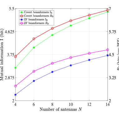
Figure 3:  The proposed covert beamformer design and proposed ZF beamformer design by  Mutual information ${\rm{I}}$ (bit) and $R_{\rm{B}}$ versus the number of antennas $N$, with the total transmit power $P_{\rm{total}}=10\rm{dBm}$ .

Fig. 3 shows the mutual information ${\rm{I}}\left({{{\bf{y}}_{\rm{R}}};{{\bf{h}}_{\rm{T}}}\left|{{s_{\rm{R}}}}\right.}\right){\rm{}}$ and $R_{\rm{B}}$ with the proposed covert beamformer design and the proposed ZF beamformer design versus the total transmit power $P_{\rm{total}}$, where the number of antennas is set as $N=5$. It can be observed that the mutual information of Radar ${\rm{I}}\left({{{\bf{y}}_{\rm{R}}};{{\bf{h}}_{\rm{T}}}\left|{{s_{\rm{R}}}}\right.}\right){\rm{}}$ and $R_{\rm{B}}$ almost linearly increase as the total available power $P_{\rm{total}}$ increases.

In Fig. 3, we plot the mutual information ${\rm{I}}\left({{{\bf{y}}_{\rm{R}}};{{\bf{h}}_{\rm{T}}}\left|{{s_{\rm{R}}}}\right.}\right){\rm{}}$ and $R_{\rm{B}}$ under the proposed covert beamformer design and the proposed ZF beamformer design versus the number of radar antennas $N$, where $P_{\rm{total}}=10\rm{dBm}$. It is observed that as the number of antennas $N$ increases, the mutual information ${\rm{I}}\left({{{\bf{y}}_{\rm{R}}};{{\bf{h}}_{\rm{T}}}\left|{{s_{\rm{R}}}}\right.}\right){\rm{}}$ and $R_{\rm{B}}$ increase in a logarithmic fashion, and the gap between the covert beamformer design and ZF beamformer design also increases. Because with more antennas, more spatial multiplexing gains can be realized. Moreover, Fig. 3 and 3 show that the covert beamforming design can achieve a larger MI and $R_{\rm{B}}$ than those of the ZF beamformer design.

V-B Imperfect WCSI

V-B1 MI Maximization

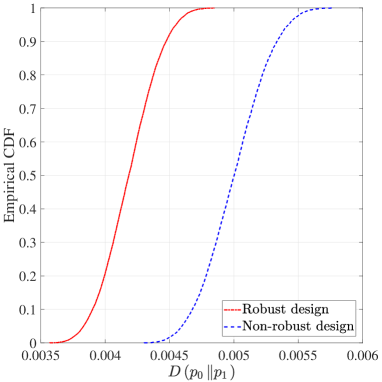
(a)

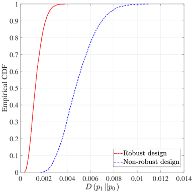
(b)

Figure 4: The empirical CDF of (a) $D\left({{p_{0}}\left\|{{p_{1}}}\right.}\right)$ and (b) $D\left({{p_{0}}\left\|{{p_{1}}}\right.}\right)$, with the covertness threshold $2{\varepsilon^{2}}=0.005$ and CSI errors $v_{w}=0.005$.

Fig. 4 (a) and (b) show the empirical CDF of the achieved $D\left({{p_{0}}\left\|{{p_{1}}}\right.}\right)$ and $D\left({{p_{1}}\left\|{{p_{0}}}\right.}\right)$ under the covertness threshold $2{\varepsilon^{2}}=0.005$ and CSI errors $v_{w}=0.005$, respectively, where $N=5$, and $P_{\rm{total}}=10\rm{dBm}$. Here, the non-robust design refers to the covert design by using the information of ${{{\bf{\hat{h}}}}_{\rm{W}}}$ only, instead of ${{{\bf{h}}}_{\rm{W}}}$. The covertness thresholds of the robust and non-robust designs are both $2{\varepsilon^{2}}=0.005$, i.e., $D\left({{p_{0}}\left\|{{p_{1}}}\right.}\right)\leq 0.005$ and $D\left({{p_{1}}\left\|{{p_{0}}}\right.}\right)\leq 0.005$. It can be seen that the CDF of the KL divergence of the non-robust design does not satisfy the constraints, where about 50% of the resulting $D\left({{p_{0}}\left\|{{p_{1}}}\right.}\right)$ exceed the covertness threshold 0.005; and about 57% of the resulting $D\left({{p_{1}}\left\|{{p_{0}}}\right.}\right)$ exceed the covertness threshold 0.005. On the other hand, the robust beamforming design guarantees the KL divergence requirement, that is, it satisfies Willie’s error detection probability requirement. In general, Fig. 4 (a) and (b) demonstrate the effectiveness of the proposed robust design.

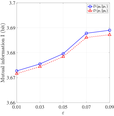
(a)

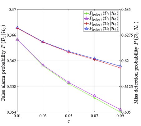
(b)

Figure 5: The value of $\varepsilon$ versus (a) the mutual information $\rm{I}$ and (b) the detection error probabilities with CSI errors $v_{w}=0.001$.

Fig. 5 (a) and (b) show the value of $\varepsilon$ versus the mutual information ${\rm{I}}\left({{{\bf{y}}_{\rm{R}}};{{\bf{h}}_{\rm{T}}}\left|{{s_{\rm{R}}}}\right.}\right){\rm{}}$ and the detection error probabilities under the two KL divergence cases, where CSI errors $v_{w}=0.001$. Fig. 5 (a) plots the mutual information ${\rm{I}}\left({{{\bf{y}}_{\rm{R}}};{{\bf{h}}_{\rm{T}}}\left|{{s_{\rm{R}}}}\right.}\right){\rm{}}$ versus the value of $\varepsilon$ under two covertness constraints $D\left({{p_{0}}\left\|{{p_{1}}}\right.}\right)\leq 2{\varepsilon^{2}}$ and $D\left({{p_{1}}\left\|{{p_{0}}}\right.}\right)\leq 2{\varepsilon^{2}}$, where CSI errors $v_{w}=0.001$. This simulation result is consistent with the theoretical analysis, that is, when $\varepsilon$ becomes larger, the covertness constraint becomes loose, which leads to a larger ${\rm{I}}\left({{{\bf{y}}_{\rm{R}}};{{\bf{h}}_{\rm{T}}}\left|{{s_{\rm{R}}}}\right.}\right){\rm{}}$. On the other hand, ${\rm{I}}\left({{{\bf{y}}_{\rm{R}}};{{\bf{h}}_{\rm{T}}}\left|{{s_{\rm{R}}}}\right.}\right){\rm{}}$ under the covertness constraints $D\left({{p_{0}}\left\|{{p_{1}}}\right.}\right)\leq 2{\varepsilon^{2}}$ is higher than that under the constraint $D\left({{p_{1}}\left\|{{p_{0}}}\right.}\right)\leq 2{\varepsilon^{2}}$. Fig. 5 (b) plots the detection error probabilities for the two KL divergence cases versus $\varepsilon$ , where CSI errors $v_{w}=0.001$. Here ${P_{\left({{p_{0}}\left\|{{p_{1}}}\right.}\right)}}\left({{{\cal D}_{1}}\left|{{{\cal H}_{0}}}\right.}\right)$ represents the FA probability $P\left({{{\cal D}_{1}}\left|{{{\cal H}_{0}}}\right.}\right)$ in the case of $D\left({{p_{0}}\left\|{{p_{1}}}\right.}\right)\leq 2{\varepsilon^{2}}$, and the other notation is defined similarly. It is found that under the two cases of the covertness constraint, the FA probability $P\left({{{\cal D}_{1}}\left|{{{\cal H}_{0}}}\right.}\right)$ and the MD probability $P\left({{{\cal D}_{0}}\left|{{{\cal H}_{1}}}\right.}\right)$ decrease as $\varepsilon$ increases, where $P\left({{{\cal D}_{1}}\left|{{{\cal H}_{0}}}\right.}\right)$ is always lower than $P\left({{{\cal D}_{0}}\left|{{{\cal H}_{1}}}\right.}\right)$. This shows that the looser the covertness constraint is, the better Willie’s detection performance will be. In addition, Fig. 5 (b) also verifies the effectiveness of the proposed robust beamformer design in covert communication.

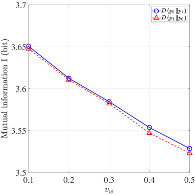
(a)

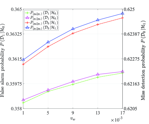
(b)

Figure 6: (a) The mutual information $\rm{I}$ versus CSI errors $v_{w}$ with the value of $\varepsilon=0.01$ and (b) the detection error probabilities versus CSI errors $v_{w}$ with the value of $\varepsilon=0.05$.

Fig. 6 (a) and (b) show CSI errors $v_{w}$ versus the mutual information ${\rm{I}}\left({{{\bf{y}}_{\rm{R}}};{{\bf{h}}_{\rm{T}}}\left|{{s_{\rm{R}}}}\right.}\right){\rm{}}$ and the detection error probabilities under the two covertness constraints $D\left({{p_{0}}\left\|{{p_{1}}}\right.}\right)\leq 2{\varepsilon^{2}}$ and $D\left({{p_{1}}\left\|{{p_{0}}}\right.}\right)\leq 2{\varepsilon^{2}}$, where the value of $\varepsilon=0.01$, $\varepsilon=0.05$, respectively. Fig. 6 (a) plots the mutual information ${\rm{I}}\left({{{\bf{y}}_{\rm{R}}};{{\bf{h}}_{\rm{T}}}\left|{{s_{\rm{R}}}}\right.}\right){\rm{}}$ versus CSI errors $v_{w}$ for the two KL divergence cases. It can be seen that the higher the CSI error is, the higher the mutual information ${\rm{I}}\left({{{\bf{y}}_{\rm{R}}};{{\bf{h}}_{\rm{T}}}\left|{{s_{\rm{R}}}}\right.}\right){\rm{}}$ and the worse radar performance will be. Fig. 6 (b) plots the FA probability $P\left({{{\cal D}_{1}}\left|{{{\cal H}_{0}}}\right.}\right)$ and the MD probability $P\left({{{\cal D}_{0}}\left|{{{\cal H}_{1}}}\right.}\right)$ versus CSI errors $v_{w}$ under two covertness constraints $D\left({{p_{0}}\left\|{{p_{1}}}\right.}\right)\leq 2{\varepsilon^{2}}$ and $D\left({{p_{1}}\left\|{{p_{0}}}\right.}\right)\leq 2{\varepsilon^{2}}$, where the value of $\varepsilon=0.05$. We observe that under the two covertness constraints, the FA probability $P\left({{{\cal D}_{1}}\left|{{{\cal H}_{0}}}\right.}\right)$ and the MD probability $P\left({{{\cal D}_{0}}\left|{{{\cal H}_{1}}}\right.}\right)$ both increase with the increase of $v_{w}$, where $P\left({{{\cal D}_{1}}\left|{{{\cal H}_{0}}}\right.}\right)$ is always less than $P\left({{{\cal D}_{0}}\left|{{{\cal H}_{1}}}\right.}\right)$. Moreover, Fig. 6 implies that a large error $v_{w}$ may lead to a good beamformer design in terms of radar performance and this beamformer may interfere with Willie’s detection, which is also beneficial to Bob. The intuition is that when the CSI error is large, the detection performance at Willie clearly would degrade.

Figure 7: The mutual information $\rm{I}$ versus number of antennas $N$ with CSI errors $v_{w}=0.005$, $\varepsilon=0.05$.

Figure 8: The mutual information $\rm{I}$ versus covert rates threshold $\beta$ with CSI errors $v_{w}=0.005$, $\varepsilon=0.05$.

Fig. 8 shows the mutual information ${\rm{I}}\left({{{\bf{y}}_{\rm{R}}};{{\bf{h}}_{\rm{T}}}\left|{{s_{\rm{R}}}}\right.}\right){\rm{}}$ versus the number of antennas $N$ under two covertness constraints $D\left({{p_{0}}\left\|{{p_{1}}}\right.}\right)\leq 2{\varepsilon^{2}}$ and $D\left({{p_{1}}\left\|{{p_{0}}}\right.}\right)\leq 2{\varepsilon^{2}}$, where $v_{w}=0.005$, $\varepsilon=0.05$. From Fig. 8, we can see that the higher the number of antennas $N$ is, the higher the mutual information ${\rm{I}}\left({{{\bf{y}}_{\rm{R}}};{{\bf{h}}_{\rm{T}}}\left|{{s_{\rm{R}}}}\right.}\right){\rm{}}$ will be, which is similar to the case in Fig. 3.

Finally, Fig. 8 shows the MI ${\rm{I}}\left({{{\bf{y}}_{\rm{R}}};{{\bf{h}}_{\rm{T}}}\left|{{s_{\rm{R}}}}\right.}\right){\rm{}}$ versus covert rates threshold $\beta$ under two covertness constraints $D\left({{p_{0}}\left\|{{p_{1}}}\right.}\right)\leq 2{\varepsilon^{2}}$ and $D\left({{p_{1}}\left\|{{p_{0}}}\right.}\right)\leq 2{\varepsilon^{2}}$, where $v_{w}=0.001$, $\varepsilon=0.05$. We can see that as the covert rate threshold $\beta$ increases, the mutual information ${\rm{I}}\left({{{\bf{y}}_{\rm{R}}};{{\bf{h}}_{\rm{T}}}\left|{{s_{\rm{R}}}}\right.}\right){\rm{}}$ gradually decreases. Moreover, from Fig. 5-8, we observe that the mutual information $\rm{I}$ with the covertness constraint $D\left({{p_{0}}\left\|{{p_{1}}}\right.}\right)\leq 2{\varepsilon^{2}}$ is higher than that with the covertness constraint $D\left({{p_{1}}\left\|{{p_{0}}}\right.}\right)\leq 2{\varepsilon^{2}}$. This is because $D\left({{p_{1}}\left\|{{p_{0}}}\right.}\right)\leq 2{\varepsilon^{2}}$ is stricter than $D\left({{p_{0}}\left\|{{p_{1}}}\right.}\right)\leq 2{\varepsilon^{2}}$, and this conclusion is in line with [34].

V-B2 Rate Maximization

In this subsection, we set $N=5$ and $P_{\rm{total}}=10\rm{dBm}$.

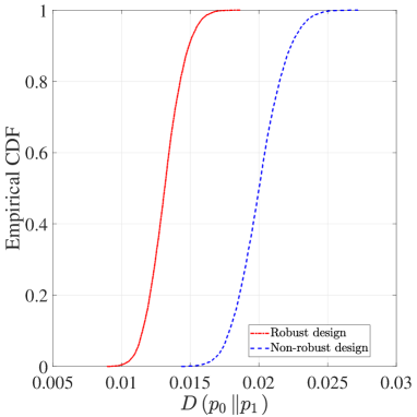
(a)

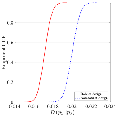
(b)

Figure 9: The empirical CDF of (a) $D\left({{p_{0}}\left\|{{p_{1}}}\right.}\right)$ and (b) $D\left({{p_{0}}\left\|{{p_{1}}}\right.}\right)$, with the covertness threshold $2{\varepsilon^{2}}=0.02$ and CSI errors $v_{w}=0.001$.

Fig. 9 (a) and (b) show the empirical CDF of the achieved $D\left({{p_{0}}\left\|{{p_{1}}}\right.}\right)$ and $D\left({{p_{1}}\left\|{{p_{0}}}\right.}\right)$ under the covertness threshold $2{\varepsilon^{2}}=0.02$ and CWSI errors $v_{w}=0.001$, respectively. The covertness threshold of the robust and non-robust designs are both $2{\varepsilon^{2}}=0.02$, i.e., $D\left({{p_{0}}\left\|{{p_{1}}}\right.}\right)\leq 0.02$ and $D\left({{p_{1}}\left\|{{p_{0}}}\right.}\right)\leq 0.02$. It can be seen that the CDF of the KL divergence of the non-robust design cannot satisfy the constraints. On the other hand, the robust beamforming design guarantees the KL divergence requirement, that is, it satisfies Willie’s error detection probability requirement. Here, the non-robust design refers to the proposed covert design with ${{{\bf{\hat{h}}}}_{\rm{W}}}$ under the same conditions. In general, Fig. 9 (a) and (b) demonstrate the effectiveness of the proposed robust design.

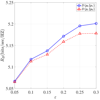
(a)

(b)

Figure 10: The value of $\varepsilon$ versus (a) the covert rate and (b) the detection error probabilities with CSI errors $v_{w}=0.001$.

Fig. 10 (a) and (b) show the value of $\varepsilon$ versus the covert rate $R_{\rm{B}}$ and the detection error probabilities under the two KL divergence cases, where CSI errors $v_{w}=0.001$. Fig. 10 (a) plots covert rates $R_{\rm{B}}$ versus $\varepsilon$ under two covertness constraints $D\left({{p_{0}}\left\|{{p_{1}}}\right.}\right)\leq 2{\varepsilon^{2}}$ and $D\left({{p_{1}}\left\|{{p_{0}}}\right.}\right)\leq 2{\varepsilon^{2}}$, where CSI errors $v_{w}=0.001$. This simulation result verifies the theoretical analysis that when $\varepsilon$ becomes larger, the covertness constraint becomes loose and $R_{\rm{B}}$ becomes larger. On the other hand, $R_{\rm{B}}$ under the covertness constraints $D\left({{p_{0}}\left\|{{p_{1}}}\right.}\right)\leq 2{\varepsilon^{2}}$ is higher than that under $D\left({{p_{1}}\left\|{{p_{0}}}\right.}\right)\leq 2{\varepsilon^{2}}$, which shows that $D\left({{p_{1}}\left\|{{p_{0}}}\right.}\right)\leq 2{\varepsilon^{2}}$ is a stricter covertness constraint than $D\left({{p_{0}}\left\|{{p_{1}}}\right.}\right)\leq 2{\varepsilon^{2}}$. Fig. 10 (b) plots the detection error probabilities for the two KL divergence cases versus $\varepsilon$, where CSI errors $v_{w}=0.001$. Here ${P_{\left({{p_{0}}\left\|{{p_{1}}}\right.}\right)}}\left({{{\cal D}_{1}}\left|{{{\cal H}_{0}}}\right.}\right)$ represents the FA probability $P\left({{{\cal D}_{1}}\left|{{{\cal H}_{0}}}\right.}\right)$ in the case of $D\left({{p_{0}}\left\|{{p_{1}}}\right.}\right)\leq 2{\varepsilon^{2}}$, and the other notation is defined similarly. It is found that under the two cases of the covertness constraint, the FA probability $P\left({{{\cal D}_{1}}\left|{{{\cal H}_{0}}}\right.}\right)$ and the MD probability $P\left({{{\cal D}_{0}}\left|{{{\cal H}_{1}}}\right.}\right)$ decrease as $\varepsilon$ increases, where $P\left({{{\cal D}_{1}}\left|{{{\cal H}_{0}}}\right.}\right)$ is always lower than $P\left({{{\cal D}_{0}}\left|{{{\cal H}_{1}}}\right.}\right)$. This shows that the looser the covertness constraint is, the better Willie’s detection performance will be. In addition, Fig. 10 (b) also verifies the effectiveness of the proposed robust beamformer design in covert communication.

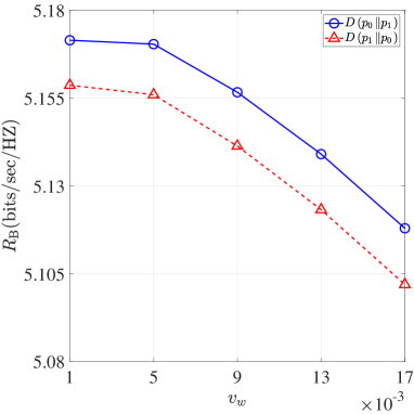
(a)

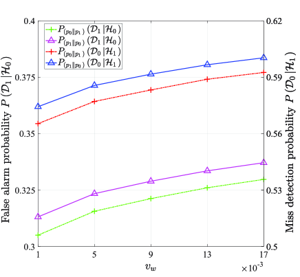
(b)

Figure 11: (a) The covert rate and (b) the detection error probabilities versus CSI errors $v_{w}$ with the value of $\varepsilon=0.20$.

Fig. 11 (a) and (b) show CSI errors $v_{w}$ versus the covert rate $R_{\rm{B}}$ and the detection error probabilities under the two covertness constraints $D\left({{p_{0}}\left\|{{p_{1}}}\right.}\right)\leq 2{\varepsilon^{2}}$ and $D\left({{p_{1}}\left\|{{p_{0}}}\right.}\right)\leq 2{\varepsilon^{2}}$, where the value of $\varepsilon=0.20$. Fig. 11 (a) plots covert rates $R_{\rm{B}}$ versus CSI errors $v_{w}$ for the two KL divergence cases. It can be seen that the higher the CSI error is, the lower the covert rate $R_{\rm{B}}$ will be. Fig. 11 (b) plots the FA probability $P\left({{{\cal D}_{1}}\left|{{{\cal H}_{0}}}\right.}\right)$ and the MD probability $P\left({{{\cal D}_{0}}\left|{{{\cal H}_{1}}}\right.}\right)$ versus CSI errors $v_{w}$ under the two covertness constraints $D\left({{p_{0}}\left\|{{p_{1}}}\right.}\right)\leq 2{\varepsilon^{2}}$ and $D\left({{p_{1}}\left\|{{p_{0}}}\right.}\right)\leq 2{\varepsilon^{2}}$, where the value of $\varepsilon=0.05$. We observe that under the two covertness constraints, the FA probability $P\left({{{\cal D}_{1}}\left|{{{\cal H}_{0}}}\right.}\right)$ and the MD probability $P\left({{{\cal D}_{0}}\left|{{{\cal H}_{1}}}\right.}\right)$ both increase with the increase of $v_{w}$, where $P\left({{{\cal D}_{1}}\left|{{{\cal H}_{0}}}\right.}\right)$ is always less than $P\left({{{\cal D}_{0}}\left|{{{\cal H}_{1}}}\right.}\right)$. Similar to the case of MI maximization, a large error $v_{w}$ may lead to a worse detection performance for Willie.

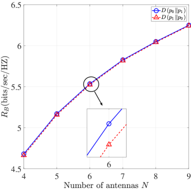
Figure 12: Covert rates $R_{\rm{B}}$ versus number of antennas $N$ with CSI errors $v_{w}=0.001$, $\varepsilon=0.20$.

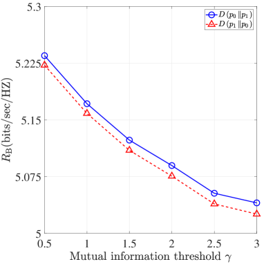
Figure 13: Covert rates $R_{\rm{B}}$ versus mutual information threshold $\gamma$ with CSI errors $v_{w}=0.001$, $\varepsilon=0.20$.

Fig. 13 shows the covert rate $R_{\rm{B}}$ versus the number of antennas $N$ under the two covertness constraints $D\left({{p_{0}}\left\|{{p_{1}}}\right.}\right)\leq 2{\varepsilon^{2}}$ and $D\left({{p_{1}}\left\|{{p_{0}}}\right.}\right)\leq 2{\varepsilon^{2}}$, where $v_{w}=0.001$ and $\varepsilon=0.20$. From Fig. 13, we can see that the higher the number of antennas $N$ is, the higher the achieved covert rates $R_{\rm{B}}$ will be, which is similar to the case in Fig. 3. Finally, Fig. 13 shows the covert rates $R_{\rm{B}}$ versus the mutual information threshold $\gamma$ under the two covertness constraints $D\left({{p_{0}}\left\|{{p_{1}}}\right.}\right)\leq 2{\varepsilon^{2}}$ and $D\left({{p_{1}}\left\|{{p_{0}}}\right.}\right)\leq 2{\varepsilon^{2}}$, where $v_{w}=0.001$, $\varepsilon=0.2$. We can see that as the mutual information threshold $\gamma$ increases, the covert rates $R_{\rm{B}}$ gradually decreases. Moreover, From Fig. 10-13, we observe that the rates with the covertness constraint $D\left({{p_{0}}\left\|{{p_{1}}}\right.}\right)\leq 2{\varepsilon^{2}}$ are higher than those with the covertness constraint $D\left({{p_{1}}\left\|{{p_{0}}}\right.}\right)\leq 2{\varepsilon^{2}}$. This is because $D\left({{p_{1}}\left\|{{p_{0}}}\right.}\right)\leq 2{\varepsilon^{2}}$ is stricter than $D\left({{p_{0}}\left\|{{p_{1}}}\right.}\right)\leq 2{\varepsilon^{2}}$, and this conclusion is also verified in [34].

VI Conclusions

In this paper, we developed a covert beamforming design framework for IRSC systems. Specifically, we proposed two effective solutions to maximize the MI of the radar while meeting the covertness requirements and the total power constraints to ensure covert transmission. When the WCSI is accurately known, we proposed a single-iterative beamforming design method based on the zero forcing criterion. When the WCSI can only be estimated with error, we proposed a robust optimization method to ensure the worst-case covert IRSC performance. Finally, simulation results showed that the proposed covert beamforming design framework can simultaneously realize radar detection and covert communication for perfect and imperfect WCSI scenarios.

References

- [1] F. Liu, C. Masouros, A. P. Petropulu, H. Griffiths, and L. Hanzo, “Joint radar and communication design: Applications, state-of-the-art, and the road ahead,” IEEE Trans. Commun., vol. 68, no. 6, pp. 3834–3862, Jun. 2020.
- [2] H. Wymeersch, G. Seco-Granados, G. Destino, D. Dardari, and F. Tufvesson, “5G mmwave positioning for vehicular networks,” IEEE Wireless Commun., vol. 24, no. 6, pp. 80–86, Dec. 2017.
- [3] F. Liu and C. Masouros, “A tutorial on joint radar and communication transmission for vehicular networks Part I: Background and fundamentals,” IEEE Commun. Lett., vol. 25, no. 2, pp. 322–326, Feb. 2021.
- [4] A. H. Lashkari, B. Parhizkar, and M. N. A. Ngan, “WIFI-Based indoor positioning system,” in Second International Conference on Computer and Network Technology (ICCNT2010), pp. 76–78, Jan. 2010.
- [5] P. M. McCormick, B. Ravenscroft, S. D. Blunt, A. J. Duly, and J. G. Metcalf, “Simultaneous radar and communication emissions from a common aperture, part ii: Experimentation,” in IEEE Radar Conf. (RadarConf), pp. 1697–1702, June. 2017.
- [6] A. Hassanien, M. G. Amin, Y. D. Zhang, and F. Ahmad, “Signaling strategies for dual-function radar communications: an overview,” IEEE Aerosp. Electron. Syst. Mag., vol. 31, no. 10, pp. 36–45, Oct. 2016.
- [7] F. Liu, L. Zhou, C. Masouros, A. Li, W. Luo, and A. Petropulu, “Toward dual-functional radar-communication systems: Optimal waveform design,” IEEE Trans. Signal Process., vol. 66, no. 16, pp. 4264–4279, Aug. 2018.
- [8] B. Li and A. P. Petropulu, “Joint transmit designs for coexistence of MIMO wireless communications and sparse sensing radars in clutter,” IEEE Trans. Aerosp. Electron. Syst., vol. 53, no. 6, pp. 2846–2864, Dec. 2017.
- [9] L. Zhou, F. Liu, C. Tian, C. Masouros, A. Li, W. Jiang, and W. Luo, “Optimal waveform design for dual-functional MIMO radar-communication systems,” in Proc. IEEE/CIC Int. Conf. Commun. China (ICCC), pp. 661–665, Aug. 2018.
- [10] X. Tong, Z. Zhang, J. Wang, C. Huang, and M. Debbah, “Joint multi-user communication and sensing exploiting both signal and environment sparsity,” IEEE J. Sel. Topics Signal Process., vol. 15, no. 6, pp. 1409–1422, Nov. 2021.
- [11] A. Deligiannis, A. Daniyan, S. Lambotharan, and J. A. Chambers, “Secrecy rate optimizations for MIMO communication radar,” IEEE Trans. Aerosp. Electron. Syst., vol. 54, no. 5, pp. 2481–2492, Oct. 2018.
- [12] B. K. Chalise and M. G. Amin, “Performance tradeoff in a unified system of communications and passive radar: A secrecy capacity approach,” Digit. Signal Process., vol. 82, pp. 282–293, Nov. 2018.
- [13] F. Liu, C. Masouros, A. Li, H. Sun, and L. Hanzo, “MU-MIMO communications with MIMO radar: From co-existence to joint transmission,” IEEE Trans. Wireless Commun., vol. 17, no. 4, pp. 2755–2770, Apr. 2018.
- [14] N. Su, F. Liu, and C. Masouros, “Secure radar-communication systems with malicious targets: Integrating radar, communications and jamming functionalities,” IEEE Trans. Wireless Commun., vol. 20, no. 1, pp. 83–95, Jan. 2021.
- [15] J. Chu, R. Liu, Y. Liu, M. Li, and Q. Liu, “AN-aided secure beamforming design for dual-functional radar-communication systems,” in 2021 IEEE/CIC International Conference on Communications in China (ICCC Workshops), pp. 54–59, Jul. 2021.
- [16] W.-C. Liao, T.-H. Chang, W.-K. Ma, and C.-Y. Chi, “Qos-based transmit beamforming in the presence of eavesdroppers: An optimized artificial-noise-aided approach,” IEEE Trans. Signal Process., vol. 59, no. 3, pp. 1202–1216, Mar. 2011.
- [17] K. Shahzad and X. Zhou, “Covert wireless communications under quasi-static fading with channel uncertainty,” IEEE Trans. Inf. Forensics Security, vol. 16, pp. 1104–1116, 2021.
- [18] B. A. Bash, D. Goeckel, D. Towsley, and S. Guha, “Hiding information in noise: fundamental limits of covert wireless communication,” IEEE Commun. Mag., vol. 53, no. 12, pp. 26–31, Dec. 2015.
- [19] D. Wang, P. Qi, Y. Zhao, C. Li, W. Wu, and Z. Li, “Covert wireless communication with noise uncertainty in space-air-ground integrated vehicular networks,” IEEE Trans. Intell. Transp. Syst., pp. 1–14, Aug. 2021.
- [20] S. Ma, Y. Zhang, H. Li, J. Sun, J. Shi, H. Zhang, C. Shen, and S. Li, “Covert beamforming design for intelligent reflecting surface assisted iot networks,” IEEE Internet Things J., pp. 1–1, Sep. 2021.
- [21] C. Wang, Z. Li, and D. W. K. Ng, “Covert rate optimization of millimeter wave full-duplex communications,” IEEE Trans. Wireless Commun., pp. 1–1, Oct. 2021.
- [22] S. Ma, Y. Zhang, H. Li, S. Lu, N. Al-Dhahir, S. Zhang, and S. Li, “Robust beamforming design for covert communications,” IEEE Trans. Inf. Forensics Security, vol. 16, pp. 3026–3038, Apr. 2021.
- [23] R. Chen, Z. Li, J. Shi, L. Yang, and J. Hu, “Achieving covert communication in overlay cognitive radio networks,” IEEE Trans. Veh. Technol., vol. 69, no. 12, pp. 15113–15126, Dec. 2020.
- [24] S. D. Blunt and P. Yantham, “Waveform design for radar-embedded communications,” in Int. Waveform Diversity and Design Conf., pp. 214–218, Jun. 2007.
- [25] S. D. Blunt, J. Stiles, C. Allen, D. Deavours, and E. Perrins, “Diversity aspects of radar-embedded communications,” in Int. Conf. Electromagnetics in Advanced Applicat., pp. 439–442, Sep. 2007.
- [26] K. Shahzad, X. Zhou, and S. Yan, “Covert communication in fading channels under channel uncertainty,” in Proc. IEEE 85th Veh. Technol. Conf. (VTC Spring), pp. 1–5, Jun. 2017.
- [27] A. Khawar, A. Abdelhadi, and C. Clancy, “Target detection performance of spectrum sharing mimo radars,” IEEE Sensors J.,, vol. 15, no. 9, pp. 4928–4940, 2015.
- [28] B. K. Chalise, M. G. Amin, and B. Himed, “Performance tradeoff in a unified passive radar and communications system,” IEEE Signal Process. Lett., vol. 24, no. 9, pp. 1275–1279, Jun. 2017.
- [29] M. Bell, “Information theory and radar waveform design,” IEEE Trans. Inform. Technol., vol. 39, no. 5, pp. 1578–1597, Sep. 1993.
- [30] B. Tang and J. Li, “Spectrally constrained MIMO radar waveform design based on mutual information,” IEEE Trans. Signal Process., vol. 67, no. 3, pp. 821–834, Feb. 2019.
- [31] M. Bica, K.-W. Huang, V. Koivunen, and U. Mitra, “Mutual information based radar waveform design for joint radar and cellular communication systems,” in Proc. IEEE Int. Conf. Acoust., Speech Signal Process., pp. 3671–3675, Mar. 2016.
- [32] S. Yan, B. He, X. Zhou, Y. Cong, and A. L. Swindlehurst, “Delay-intolerant covert communications with either fixed or random transmit power,” IEEE Trans. Inf. Forensics Security, vol. 14, no. 1, pp. 129–140, Jan. 2019.
- [33] E. L. Lehmann, J. P. Romano, and G. Casella, Testing statistical hypotheses, vol. 3, Springer, 2005.
- [34] S. Yan, Y. Cong, S. V. Hanly, and X. Zhou, “Gaussian signalling for covert communications,” IEEE Trans. Wireless Commun., vol. 18, no. 7, pp. 3542–3553, Jul. 2019.
- [35] B. A. Bash, D. Goeckel, and D. Towsley, “Limits of reliable communication with low probability of detection on AWGN channels,” IEEE J. Sel. Areas Commun., vol. 31, no. 9, pp. 1921–1930, Sep. 2013.
- [36] A. Ben-Naim, Elements of Information Theory, A Farewell To Entropy:Statistical Thermodynamics Based on Information, 2014.
- [37] T. M. Cover, Elements of information theory, John Wiley & Sons, 1999.
- [38] Z.-Q. Luo, W.-K. Ma, A. M.-C. So, Y. Ye, and S. Zhang, “Semidefinite relaxation of quadratic optimization problems,” IEEE Signal Process. Mag., vol. 27, no. 3, pp. 20–34, May 2010.
- [39] M. Grant and S. Boyd, “CVX: Matlab software for disciplined convex programming, version 2.1,” http://cvxr.com/cvx, Mar. 2014.
- [40] J. F. Sturm, “Using sedumi 1.02, a matlab toolbox for optimization over symmetric cones,” Optim. Methods Softw., vol. 11, no. 1-4, pp. 625–653, 1999.
- [41] A. Vakili, M. Sharif, and B. Hassibi, “The effect of channel estimation error on the throughput of broadcast channels,” in Proc. IEEE Int. Conf. Acoust. Speed Signal Process. Proc., vol. 4, pp. 14–19, May 2006.
- [42] L. Wei, C. Huang, G. C. Alexandropoulos, and C. Yuen, “Parallel factor decomposition channel estimation in RIS-assisted multi-user MISO communication,” in 2020 IEEE 11th Sensor Array and Multichannel Signal Processing Workshop (SAM), pp. 1–5, Jun. 2020.
- [43] L. Wei, C. Huang, G. C. Alexandropoulos, C. Yuen, Z. Zhang, and M. Debbah, “Channel estimation for RIS-empowered multi-user MISO wireless communications,” IEEE Trans. Commun., vol. 69, no. 6, pp. 4144–4157, Jun. 2021.
- [44] M. Forouzesh, P. Azmi, N. Mokari, and D. Goeckel, “Covert communication using null space and 3D beamforming: Uncertainty of willie’s location information,” IEEE Trans. Veh. Technol., vol. 69, no. 8, pp. 8568–8576, Aug. 2020.
- [45] B. He and X. Zhou, “Secure on-off transmission design with channel estimation errors,” IEEE Trans. Inf. Forensics Security, vol. 8, no. 12, pp. 1923–1936, Dec. 2013.
- [46] D. W. K. Ng, E. S. Lo, and R. Schober, “Robust beamforming for secure communication in systems with wireless information and power transfer,” IEEE Trans. Wireless Commun., vol. 13, no. 8, pp. 4599–4615, Aug. 2014.
- [47] F. Liu and C. Masouros, “Joint beamforming design for extended target estimation and multiuser communication,” in 2020 IEEE Radar Conference (RadarConf20), pp. 1–6, Sep. 2020.
- [48] Z. Cheng, B. Liao, S. Shi, Z. He, and J. Li, “Co-design for overlaid MIMO radar and downlink MISO communication systems via Cramer-Rao bound minimization,” IEEE Trans. Signal Process., vol. 67, no. 24, pp. 6227–6240, Dec. 2019.