Flexible Unsupervised Learning for Massive MIMO Subarray Hybrid Beamforming

Abstract

Hybrid beamforming is a promising technology to improve the energy efficiency of massive MIMO systems. In particular, subarray hybrid beamforming can further decrease power consumption by reducing the number of phase-shifters. However, designing the hybrid beamforming vectors is a complex task due to the discrete nature of the subarray connections and the phase-shift amounts. Finding the optimal connections between RF chains and antennas requires solving a non-convex problem in a large search space. In addition, conventional solutions assume that perfect channel state information (CSI) is available, which is not the case in practical systems. Therefore, we propose a novel unsupervised learning approach to design the hybrid beamforming for any subarray structure while supporting quantized phase-shifters and noisy CSI. One major feature of the proposed architecture is that no beamforming codebook is required, and the neural network is trained to take into account the phase-shifter quantization. Simulation results show that the proposed deep learning solutions can achieve higher sum-rates than existing methods.

I Introduction

Hybrid beamforming (HBF) is a well-known approach to reduce the energy consumption of massive MIMO (mMIMO) systems through a reduction in the number of transmitting radio frequency (RF) chains obtained by employing a hybrid structure combining a phase-shift analog precoder (AP) with a baseband digital precoder (DP) transmission  [1]. As a result, HBF techniques have been considered for fifth-generation cellular networks (5G) in the millimeter wave (mm-Wave) bands, and will most likely be extended to 6G [2]. In general, three HBF structures are considered: fully-connected HBF (FC-HBF), fixed subarray HBF (FSA-HBF) and dynamic subarray HBF (DSA-HBF). In FC-HBF, all RF chains are connected to all the antennas, providing the maximum degree of freedom. This structure offers the best performance, but it requires a large number of phase-shifters (PSs) that consume a non-negligible amount of energy. In the FSA-HBF structure, RF chains are connected to a fixed subset of antennas. The number of PSs being reduced, the energy efficiency of this structure is higher than FC-HBF [3]. Finally, in DSA-HBF, the connections between RF chains and antennas can dynamically change using low power multiplexers, as proposed in [4], and enable further energy-efficiency improvements.

However, designing HBF that achieve near-optimal performance usually has a high computational cost. Recently, several works have investigated the use of deep learning (DL) to design the HBF for FC-HBF [5, 6]. To the best of our knowledge, the only DL approach for designing subarray HBF was proposed in [7], for the case of a fixed subarray. However, these works proposed a supervised learning approach with perfect CSI knowledge, where the target values need to be computed using conventional HBF algorithms that are computationally complex. These solutions are not extendable to subarray HBF due to additional constraints that need to be taken into account when designing the APs.

A more interesting approach consists in training a deep neural network (DNN) without targets, which significantly reduces the training complexity, while also making it possible to outperform the conventional approaches. An unsupervised learning method for FC-HBF was proposed in [8]. However, this solution is not extendable to subarray HBF because of the additional constraints that need to be taken into account when designing the AP. Furthermore, it is important to take into account practical system constraints to achieve the best performance. CSI must be estimated and is prone to inaccuracies, while practical phase shifters are always quantized. Existing work address PS quantization in two ways, either by designing with real-valued phase shifts and then applying quantization, or by constructing an AP codebook. The codebook approach allows optimizing directly the quantized phase shifts, but the design of the codebook can be complex since the search space grows exponentially with the number of antennas, the number of RF chains, and the PS quantization. The codebook approach also imposes a trade-off between codebook size, and the associated memory usage, and sum-rate performance.

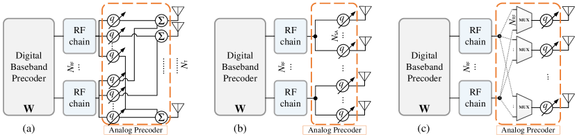
Figure 1: Hybrid Beamforming structures a) FC-HBF, b) FSA-HBF and c) DSA-HBF.

Therefore, in this paper, we propose a novel flexible unsupervised training for several HBF structures with quantized PSs that is not based on a codebook. Particularly, this is the first time an unsupervised DNN architecture is proposed for FSA-HBF and DSA-HBF. Although the DNN directly outputs quantized AP values, the DNN is properly trained and the gradient can be computed over the quantization layer. Since the training is unsupervised and no AP codebook is required, the amount of pre-processing steps required for DNN training has been simplified significantly. Moreover, we assume that the noisy pilot signal received from the users is the only information available to the DNN during inference. We demonstrate using simulation results that the proposed solutions outperform conventional methods in all considered HBF structures.

The rest of the paper is organized as follows. Section II gives the system model. In Section III, conventional methods are provided for each HBF structure. The proposed flexible unsupervised learning is described in Section IV, followed by simulation results in Section V. Section VI concludes the paper.

II System Model

We consider a multi-user mm-Wave system consisting of a mMIMO base station (BS) in a single-cell system equipped with $N_{\sf{T}}$ antennas and $N_{\sf{RF}}$ RF chains serving $N_{\sf{U}}$ single antenna users simultaneously. For both uplink and downlink transmission, HBF precoders are employed by the BS. We assumed that all employed PSs have $q$ bits quantization.

II-A Problem Definition

The main objective of this paper is to design the HBF vectors in the downlink for three different structures to maximize the sum-rate. Independently of the chosen HBF structure, the signal received by each user can be written as

$$\mathbf{y}_{u}=\mathbf{h}_{u}^{\dagger}\mathbf{A}_{q}\sum_{\forall u}\mathbf{w}_{u}x_{u}+\boldsymbol{\eta},$$ (1)

where $\mathbf{h}_{u}\in\mathbb{C}^{N_{\sf{T}}\times 1}$ stands for the channel vector from the user index $u$ to the $N_{\sf{T}}$ antennas at the BS, $\mathbf{x}=[x_{1},...,x_{u},...,x_{N_{\sf{U}}}]$ is the vectors of transmitted symbol for all users, normalized to $\mathop{\mathbb{E}}[\mathbf{x}\mathbf{x}^{\dagger}]=\frac{1}{N_{\sf{U}}}\mathbbm{1}_{N_{\sf{U}}}$, and $\boldsymbol{\eta}$ is the additive white gaussian noise (AWGN) term with noise power $\sigma^{2}$. The HBF vectors consist of a digital baseband precoder $\mathbf{W}=[\mathbf{w}_{1},...,\mathbf{w}_{u},...,\mathbf{w}_{N_{\sf{U}}}]\in\mathbb{C}^{N_{\sf{RF}}\times N_{\sf{U}}}$ and AP which is defined by a $N_{\sf{T}}\times N_{\sf{RF}}$ matrix $\mathbf{A}_{q}\in\mathbb{C}^{N_{\sf{T}}\times N_{\sf{RF}}}$, where $[\mathbf{A}_{q}]_{n,m}$ is the coefficient of the $q$ bits PS connected between the $n^{\text{th}}$ antenna and $m^{\text{th}}$ RF chain. The sum-rate for a given hybrid beamformer $(\mathbf{A}_{q},\mathbf{W})$ is given by

$$R(\mathbf{A}_{q},\mathbf{W})=\sum_{\forall u}\text{log}_{2}\Bigl{(}1+\text{SINR}(\mathbf{A}_{q},\mathbf{w}_{u})\Bigr{)}\,,$$ (2)

where the signal-to-interference-noise ratio (SINR) of the $u^{\text{th}}$ user can be expressed as

$$\text{SINR}(\mathbf{A}_{q},\mathbf{w}_{u}) =\frac{\big{|}\mathbf{h}^{\dagger}_{u}\mathbf{A}_{q}\mathbf{w}_{u}\big{|}^{2}}{\sum_{j\neq u}\big{|}\mathbf{h}^{\dagger}_{u}\mathbf{A}_{q}\mathbf{w}_{j}\big{|}^{2}+\sigma^{2}}\,.$$ (3)

Then, the HBF design consists of finding the precoder matrices $\mathbf{W}$ and $\mathbf{A}_{q}$ that maximize the sum-rate in (2) subject to a maximum transmission power $P_{\sf{max}}$ and AP constraints. More formally, we seek to solve the following optimization problem:

$$\underset{\mathbf{A}_{q},\mathbf{W}}{\max} R(\mathbf{A}_{q},\mathbf{W})=\underset{\mathbf{A}_{q},\mathbf{w}_{u}}{\max}\sum_{\forall u}\text{log}_{2}\Bigl{(}1+\text{SINR}(\mathbf{A}_{q},\mathbf{w}_{u})\Bigr{)},$$ (4a)

s.t. $$\sum_{\forall u}\mathbf{w}_{u}^{\dagger}\mathbf{A}_{q}^{\dagger}\mathbf{A}_{q}\mathbf{w}_{u}\leq P_{\sf{max}},$$

where $P_{\sf{max}}$ is the normalized transmit power constraint. The analog precoder $\mathbf{A}_{q}$ matrix depends on HBF structure described in more details in the next section.

In this paper, we consider time division duplex (TDD) communication and we assume that the channel reciprocity is available such that the uplink channel estimate can be used for the downlink transmission. We assume that the users transmit orthogonal pilots, such that the BS receives

$$\hat{\mathbf{H}}=\mathbf{H}^{{\dagger}}+\boldsymbol{\eta},$$ (5)

where $\mathbf{H}=[\mathbf{h}_{1},...,\mathbf{h}_{N_{\sf{U}}}]^{\rm{T}}$. As we explain in Section IV, the proposed DNN directly takes as input the noisy channel estimation $\hat{\mathbf{H}}$.

III Baseline Hybrid Beamforming

In this section we review the conventional (non-DL) solutions for each type of HBF structure, and describe the corresponding AP.

III-A Fully Connected Hybrid Beamforming (FC-HBF)

In FC-HBF, as shown in Fig. 1(a), each RF chain is connected to all $N_{\sf{T}}$ antennas through PSs and combiners. Considering that the PSs are quantized on $q$ bits, the set of feasible APs has size $2^{qN_{\sf{T}}N_{\sf{RF}}}$. Conventional HBF solutions either consider a codebook-based solution to limit the set of feasible solutions [9] or use real-valued PSs [10], which is not practical in a realistic system. The conventional approach consists in first designing the optimal fully digital precoder (FDP) matrix, denoted $\mathbf{U}_{\sf{opt}}=[\mathbf{u}_{1},...,\mathbf{u}_{u},...,\mathbf{u}_{N_{\sf{U}}}]$, where $N_{\sf{RF}}=N_{\sf{T}}$. Then, the AP and DP are designed in such a way that the resulting precoder approximates $\mathbf{U}_{\sf{opt}}$ as follows:

$$\underset{\mathbf{A}_{q},\mathbf{w}_{u}}{\operatorname*{minimize}}\big{\|}\mathbf{U}_{\sf{opt}}-\mathbf{A}_{q}\mathbf{w}_{u}\big{\|}^{2}\hskip 22.76219pt\text{s.t. \eqref{cnt2}},$$ (6)

Since all the antennas are connected to all the RF chains through a PS with $q$-bit quantization, we define $[\mathbf{A}_{q}]_{n,m}\in\{e^{j2\pi k/2^{q}}:k\in\{1,\dots,2^{q}\}\}$ as the feasible set for the AP. The FDP $\mathbf{U}_{\sf{opt}}$ in (6) is obtained by solving the following problem:

$$\underset{\left\{\mathbf{U}_{\sf{opt}}\right\}}{\max} \sum_{\forall u}R_{\text{FDP}}(\mathbf{U}_{\sf{opt}})$$ (7a)

s. t. $$\sum_{\forall u}\mathbf{u}_{u}^{\dagger}\mathbf{u}_{u}\leq P_{\sf{max}},$$ (7b)

where $R_{\text{FDP}}(\mathbf{U}_{\sf{opt}})=\sum_{\forall u}\log_{2}(1+\mathrm{SINR}_{u}(\mathbf{u}_{u}))\,$ and

$$\text{SINR}(\mathbf{u}_{u})=\frac{\big{|}\mathbf{h}^{\dagger}_{u}\mathbf{u}_{u}\big{|}^{2}}{\sum_{j\neq u}\big{|}\mathbf{h}^{\dagger}_{u}\mathbf{u}_{j}\big{|}^{2}+\sigma^{2}}.$$ (8)

The baseline results presented in this paper are obtained by solving (7) based on [11], and then obtaining the FC-HBF solution using “PE-AltMin” proposed in [10].

III-B Subarray Hybrid Beamforming

In subarray structures, each antenna is connected to only one RF chain through a PS. Therefore, the total number of PSs is reduced to $N_{\sf{T}}$ (instead of $N_{\sf{T}}\times N_{\sf{RF}}$). These structures can either have fixed connections, as shown in Fig. 1(b), or dynamic connections (Fig. 1(c)), where the connections between antennas and RF chains can be switched dynamically using a multiplexers network. It is shown in [4] that such dynamic structure improves the spectral efficiency of the system by providing more degrees of freedom in HBF design compared to FSA-HBF, while reducing the power consumption compared to FC-HBF. The AP in both subarray structures consists of two parts, i) PSs and ii) connections between RF chains and PSs. Therefore, the general feasible AP matrix for subarray beamforming can be written as

$$\mathbf{A}_{\text{q}}=\underbrace{\text{diag}\big{(}a_{1},...,a_{N_{\sf{T}}}\big{)}}_{\text{Phase-shifters}}\mathbf{S},$$ (9)

where $a_{i}\in\{e^{j2\pi k/2^{q}}:k\in\{1,\dots,2^{q}\}\}$, and $\mathbf{S}$ is a binary ${N_{\sf{T}}\times N_{\sf{RF}}}$ matrix ($[\mathbf{S}]_{n,m}\in\{0,1\}$) to represent the connections between the RF chains and antennas. To differentiate HBF structures, we denotes $\mathbf{S}_{\sf{FSA}}$ when the connection matrix $\mathbf{S}$ is fixed (FSA-HBF case) and $\mathbf{S}_{\sf{DSA}}$ where that matrix is variable (DSA-HBF case) and need to be jointly optimized with AP and DP. Since each antenna must be connected to only one RF chain, the constraint on matrix $\mathbf{S}$ is

$$\sum_{\forall m}[\mathbf{S}]_{n,m}=1\quad\forall\ n.$$ (10)

Some types of fixed subarray connections have been studied in [4], where it was shown that type “Squared” achieves better sum-rate than other types. Thus, we set $\mathbf{S}_{\sf{FSA}}$ to the “Squared” connection pattern. The general approach described in (6) can be considered here as well. In [7], a solution called “CR-AltMin” proposed to design the FSA-HBF. We used this method as a point of comparison for our DL solution.

For the DSA-HBF, $\mathbf{S}_{\sf{DSA}}$ needs to be optimized, resulting in a large design space. In [4], a sub-optimal method named “Dynamic Subarray Partitioning” is proposed. We consider this method as a point of comparison for our proposed unsupervised learning solution.

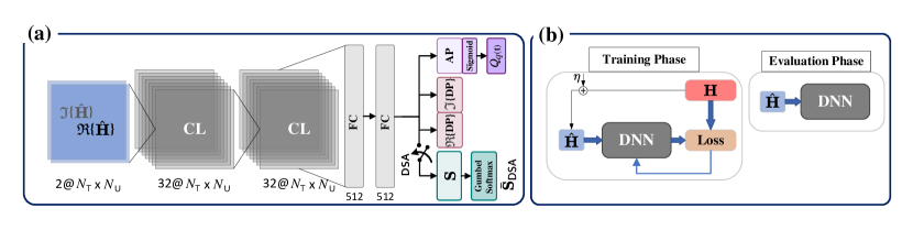
Figure 2: Proposed unsupervised learning hybrid beamforming design a) DNN architecture, b) Training and evaluation procedure of DNN.

IV Proposed Flexible Unsupervised Training for Subarray Hybrid Beamforming

In this section, we describe a DL architecture for designing the HBF for fully connected and subarray structures. The training (offline) and evaluation (online) phases are detailed. All proposed DL techniques are unsupervised. This is challenging because, in contrast with supervised DL, training the DNN for each subarray structure requires different algorithms, since different hardware constraints must be considered.

IV-A Network Architecture

The proposed DNN architecture is shown in Fig. 2 (a) and consists of $2$ convolutional layers (CLs) $32@N_{\sf{T}}\times N_{\sf{U}}$ where $32$ is the number of channel and $N_{\sf{T}}\times N_{\sf{U}}$ is the dimension of each channel. The kernel size is $3\times 3$ for all CLs. The CLs are followed by $2$ fully-connected layers (FLs), each with $512$ neurons, and by an output layer. The “Leaky ReLU” activation function is employed after all layers, except the output layer. Batch normalization is used after each layer to avoid over-fitting. The input of the DNN is the noisy channel matrix $\hat{\mathbf{H}}$ as described in Section II. To improve the representation learning, we separate the real and imaginary part of $\hat{\mathbf{H}}$, respectively denoted $\Re\{\hat{\mathbf{H}}\}$ and $\Im\{\hat{\mathbf{H}}\}$, into two channels in the first CL. We divide the output of the last FL into $4$ parallel layers. The output of the first parallel layer generates the AP, thus its dimension is $N_{\sf{RF}}\times N_{\sf{T}}$ for FC-HBF and $N_{\sf{T}}$ for both FSA-HBF and DSA-HBF. It is followed by a “Sigmoid” activation function that scales the components of the tensor in the range $[0,1]$, and then by the quantization function $Q_{q}$ that outputs the phase of the PSs, defined as:

$$Q_{q}(t)=2\pi\lceil t2^{q}\rceil/2^{q}\quad\,$$ (11)

where $\lceil x\rceil$ denotes the smallest integer greater or equal to $x$ and $t$ is an activation value. The second and third parallel layers, both of size ${N_{\sf{RF}}\times N_{\sf{U}}}$, respectively generate the real and imaginary part of the DP. Finally, the fourth layer of size ${N_{\sf{RF}}\times N_{\sf{T}}}$ is only activated for the DSA-HBF structure and designs the multiplexer network. We considered the “Gumbel-Softmax” activation function [12] to satisfy the constraint described in (10). More details will be given in Section IV-B3 regarding this choice.

IV-B Unsupervised Training

The training phase procedure is shown in Fig. 2 (b) (labeled “Training Phase”). During training, we assume the CSI is only available to measure the performance of the DNN through the loss function. The input of the DNN only has access to a noisy version of the CSI. Therefore, the training dataset is only composed of $\mathbf{H}$ matrix samples. These samples can be collected, for instance, during an initial “offline” phase where the channel environment is sounded. During this phase, more bandwidth resources can be dedicated toward CSI acquisition to improve the estimation accuracy.

In the training phase (offline), the weights and biases are tuned based on a defined loss function, and back propagation computes the gradient over each layer. The use of quantization functions during training is forbidden because it is not differentiable and therefore breaks the back propagation graph. To solve this issue, [13] proposes to use a differentiable activation function for $1$ bit PSs. However, this method does not scale well to a higher number of bits, as we discuss later in Section V. In this paper, we instead rely on the straight through estimator (STE) technique [14]. The quantization function (11) is only activated in the forward pass, and the output activation values are constrained in the range $[0,2\pi]$. In the backward pass, the gradient is simply passed through unchanged. In what follows we describe the training of each structure.

IV-B1 Fully Connected Hybrid Beamforming (FC-HBF-Net)

In FC-HBF, as we described in Section III, $[\mathbf{A}_{q}]_{n,m}\in\{e^{j2\pi k/2^{q}}:k\in\{1,\dots,2^{q}\}\}$. Therefore, considering that $\bar{\mathbf{A}}_{q}$ and $\bar{\mathbf{W}}$ are the output of the quantized AP and DP, respectively, the loss function can be written as

$$\mathcal{L}=-R(\bar{\mathbf{A}}_{q},\bar{\mathbf{W}}),$$ (12)

where $R$ denotes the sum-rate defined in (2).

IV-B2 Fixed Subarray Hybrid Beamforming (FSA-HBF-Net)

The loss function used for the FSA-HBF structure is also given by (12). However, $\bar{\mathbf{A}}_{q}$ is constrained to be of the form given by (9), where $\mathbf{S}=\mathbf{S_{\sf{FSA}}}$, and $\mathbf{S_{\sf{FSA}}}$ corresponds to the “Squared” connection defined in [4].

IV-B3 Dynamic Subarray Hybrid Beamforming (DSA-HBF-Net)

The training procedure of DSA-HBF is more challenging than the two previous structures since the matrix $\mathbf{S_{\sf{DSA}}}$ becomes an additional variable to be jointly optimized with the $\mathbf{A}_{q}$ and $\mathbf{W}$ matrices. According to the subarray constraint defined in (10), each antenna must be connected to only one RF chain at any given time. Note that each RF chain can still be connected to multiple antennas. Therefore, $\mathbf{S_{\sf{DSA}}}$ can be seen as a concatenation of $N_{\sf{T}}$ “one-hot” vectors, each of length $N_{\sf{RF}}$, where a “one-hot” vector is defined as a binary vector with a Hamming weight of $1$. In classification tasks, the need to choose one of many categories is typically handled by applying the “softmax” function during training, which is replaced by a (hard) maximum during the test phase. However, we found that this approach does not lead to good results for unsupervised learning, because the sum rate measured during training can then be very different from the actual test-time sum rate. To solve this issue, we propose a differentiable approximation during training inspired by the “Gumbel-Softmax” estimator [12]. Gumbel-Softmax is a technique that allows sampling from a categorical distribution during the forward pass of a neural network, by combining the reparameterization trick and smooth relaxation. Defining $p_{i,j}$ the probability that antenna $i$ is connected to RF chains $j$, we can form a $1\times N_{\sf{RF}}$ vector $\mathbf{p}_{i}=[p_{i,1},...,p_{i,N_{\sf{RF}}}]$ that corresponds to the probability states between antenna $i$ and all RF chains. Note that $\sum_{j}p_{i,j}=1\;\forall i\in[1,N_{\sf{T}}]$ due to constraint (10). The Gumbel-Softmax function applied to that vector, $G(\mathbf{p}_{i})$, can then be defined as

$$G(\mathbf{p}_{i})=\frac{\exp((\log(\mathbf{p}_{i})+g_{i})/\tau)}{\sum_{j=1}^{N_{\sf{RF}}}\exp((\log(p_{i,j})+g_{i,j})/\tau)},$$ (13)

where $g_{i,j}$ is a sample drawn from Gumbel distribution [15] with mean $0$ and variance $1$. Note that the $\exp(.)$ and $\log(.)$ functions are applied element-wise when taking a vector as input. The parameter $\tau$ is called “Softmax temperature”. When $\tau\rightarrow 0$, $G(\mathbf{p}_{i})$ tends to the categorical distribution, but when $\tau\rightarrow\infty$, it converges to the uniform distribution [12]. There is a trade-off between small temperatures, where sample vectors are close to one-hot but the variance of the gradient is large, and large temperatures, where samples are more uniform but the variance of the gradient is small. We thus consider $\tau$ as a hyper-parameter to be optimized. Finally, the output of the fourth layer, denoted $\bar{\mathbf{S}}_{\sf{DSA}}$, is obtained after a row-concatenation of vectors $G(\mathbf{p}_{i})\;\forall i\in[1,N_{\sf{T}}]$. The analog precoder $\bar{\mathbf{A}}_{q}$ is obtained from (9), where $\mathbf{S}$ is replaced by $\bar{\mathbf{S}}_{\sf{DSA}}$, and the loss function (12) can be computed. For the power constraint, we assumed a fixed transmit power for each RF chain. Then, the power of each RF chain is split equally among the antennas it is connected to. Furthermore, the total transmit power by AP and DP is normalized to satisfy the power constraint in (4a).

IV-C Evaluation Phase

In the evaluation phase, the DNN input consists only of noisy channel matrices $\hat{\mathbf{H}}$. In all three HBF structures, the output of the AP is quantized based on (11), whereas the DP can be used directly since it is continuous. For the DSA-HBF structure, the multiplexer network in evaluation phase can be obtained by

$$[\mathbf{S}_{\sf{DSA}}]_{i,j}=\begin{cases}1,&\text{if $j=\operatorname*{arg\;max}_{j^{\prime}}(p_{i,j^{\prime}})$,}\\ 0,&\text{otherwise.}\end{cases}$$ (14)

The form of (14) is known as “one-hot encoding,” and it determines the dynamic connection between the antennas and RF chains while ensuring that (10) is satisfied.

TABLE I: Sum-Rate Comparison of Proposed method

		Beamforming		Sum-Rate
Technique	CSI Status	structure	# Phase-Shifter	(bit/s/Hz)
O-FDP	Perfect CSI	FDP	-	$22.8$
FC-HBF-Net	Noisy CSI	FC-HBF	$N_{\sf{RF}}N_{\sf{T}}$	21.7
MO-AltMin [10]	Perfect CSI	FC-HBF	$N_{\sf{RF}}N_{\sf{T}}$	$18.9$
PE-AltMin [10]	Perfect CSI	FC-HBF	$N_{\sf{RF}}N_{\sf{T}}$	$17.8$
OMP [9]	Perfect CSI	FC-HBF	$N_{\sf{RF}}N_{\sf{T}}$	$15$
DSA-HBF-Net	Noisy CSI	DSA-HBF	$N_{\sf{T}}$	20.1
Park, et al [4]	Perfect CSI	DSA-HBF	$N_{\sf{T}}$	$18.7$
FSA-HBF-Net	Noisy CSI	FSA-HBF	$N_{\sf{T}}$	16.4
CR-AltMin [7]	Perfect CSI	FSA-HBF	$N_{\sf{T}}$	$13.8$
($N_{\sf{T}}=64$, $N_{\sf{RF}}=8$, $N_{\sf{U}}=4$, $\sigma^{2}=-130$ dBW)

V Numerical Results

The performance of the proposed solutions have been evaluated numerically by using the PyTorch DL framework. Scenario “O1-$28$ GHz” of the deepMIMO channel model [16] is employed to generate the dataset. The BS is equipped with $N_{\sf{T}}=64$ antennas and $N_{\sf{RF}}=8$ RF chains with $q$-bit PSs serving $N_{\sf{U}}=4$ users located randomly in a dedicated area (in deepMIMO channel model $\texttt{active\_user\_first}=1100$ and $\texttt{active\_user\_last}=2200$). The size of the DNN dataset is set to $2\times 10^{6}$ samples, with $85$% of the samples used for the training set and the remaining ones used to evaluate the performance. The mini-batch size, learning rate, and weight decay are set to $1000$, $0.001$, and $10^{-5}$, respectively. We used “RAdam” as the DNN training optimizer [17]. The training procedure converged after approximately $200$ epochs.

Table I compares the sum-rate performance of all techniques. The best sum-rate is obtained by O-FDP since the RF structure is not constrained, but this solution is not energy-efficient compared to HBF. The DNN architecture implementing the FC-HBF structure achieves $95\%$ of FDP sum-rate, while improving the sum-rate by $15\%$ when compared to the MO-AltMin solution [10]. FSA-HBF-Net outperforms existing methods by $19\%$. Furthermore, the DSA-HBF-Net approximately reaches $92\%$ of FC-HBF sum-rate, while the number of PSs has been divided by a factor $N_{\sf{RF}}$. For DSA-HBF-Net, the Gumbel-Softmax temperature is set to $\tau=1.5$. This choice will be motivated later in this section. When compared to “Dynamic Subarray Partitioning” in [4], the proposed approach improves the sum-rate by $7\%$. Note that all conventional methods were evaluated using perfect CSI, whereas the proposed DNN techniques consider noisy CSI in the evaluation phase. Therefore, it is expected that the performance gap would be larger in practice.

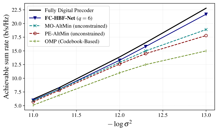
Figure 3: Sum-rate performance of FC-HBF.

Fig. 3 shows the sum-rate performance of FC-HBF based solutions for different noise power values $\sigma^{2}$. Sum-rate of the optimal FDP solution is also shown and provides an upper-bound for the sum-rate performance. Taking into account channel attenuation, the average signal-to-noise ratios (SNRs) ranges from $6.7$ dB to $26.7$ dB. The proposed FC-HBF-Net outperforms all conventional FC-HBF solutions for all noise power. Note that the performance gap between FDP and HBF increases at low noise power due to residual interference being more dominant for HBF systems.

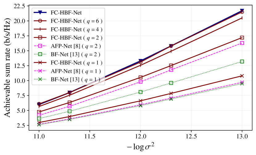
Figure 4: Sum-rate of DL-Based HBF with different PS quantization bits.

Fig. 4 shows the impact of the PS quantization on the sum-rate performance. We consider PS representations from 1 to 6 bits. At 6 bits, the sum-rate becomes almost identical to the ideal case of continuous phase shifts. As a comparison for the proposed approach, Fig. 4 also reports the sum-rate achieved by the codebook-based solution “AFP-Net” [8], for 1 and 2-bit PS quantization. It can be seen that the codebook-based solution provides lower sum-rate since its performance is limited by the codebook design. In contrast, the proposed DL solution directly finds the optimal solution. We also compare against an existing 1-bit quantization method trained using a differentiable function [13], that we adapted to also support a 2-bit quantization. These reference curves are labeled “BF-Net” in Fig. 4. To evaluate the performance on our dataset, we replaced our quantization function with the one from [13], taking care to re-optimize the method’s $\alpha$ parameter since it could depend on the DNN architecture and channel model. We observed that $\alpha=0.1$ is the best trade-off between the training and evaluation loss for $q\in\{1,2\}$. It can be seen that the use of the STE quantization trick allows the proposed DNN to be trained properly while supporting any PS quantization, and that our approach outperforms the quantization method in [13]. Particularly, the performance gap is significantly higher at $q=2$, which tends to show that the method proposed in [13] does not scale well when increasing the number of quantization bits.

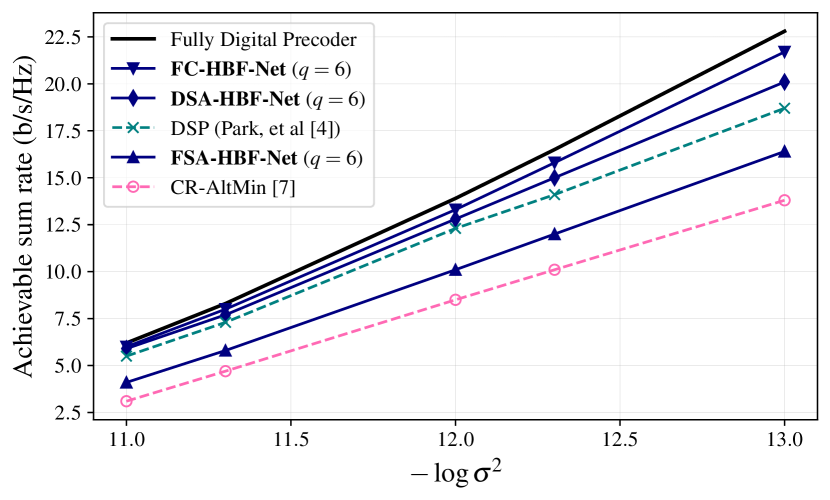
Figure 5: Sum-rate performance of FC-HBF, FSA-HBF, and DSA-HBF.

Fig. 5 shows the obtained sum-rate performance when considering different HBF structures. FC-HBF being the less constrained structure, it achieves the highest sum-rate performance. The most constrained structure, FSA-HBF, reduces the power consumption of the RF phase-shifter array at the cost of offering the worst sum-rate performance. The sum-rate performance of the DSA-HBF is very close to FC-HBF while only requiring $N_{\sf{T}}$ PSs. The multiplexer network improves the HBF design flexibility, which in turn improves the sum-rate when compared to FSA-HBF.

Finally, we evaluate in Fig. 6 how the Gumbel-Softmax temperature $\tau$ impacts the sum-rate performance of DSA-HBF-Net during the evaluation and training phases, for different noise powers. To improve the clarity of the figure, we normalize the sum-rate using $R/R^{\star}$, where $R^{\star}$ is the maximum sum-rate achieved at each noise power during the evaluation phase. We can observe that the best evaluation-phase sum-rate among the search options is obtained at $\tau=1.5$ for all noise powers. Note that for higher $\tau$ values, the sum-rate performance of the training phase keeps improving, while the sum-rate is significantly degraded in the evaluation phase. This is due to the fact that Gumbel-Softmax converges toward a uniform distribution for large $\tau$, and therefore becomes a bad representation of the desired one-hot vector.

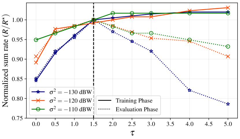
Figure 6: Sum-rate performance of DSA-HBF versus different $\tau$.

VI Conclusion

Subarray hybrid beamforming enables to further improve the energy efficiency of conventional HBF by reducing the number of phase-shifters. We propose for the first time an unsupervised DNN architecture for FSA-HBF and DSA-HBF, while supporting quantized phase shifters of any resolution. Since quantization functions are not differentiable and, consequently, cannot be used in back propagation, we considered the STE technique to train the network with quantized PSs. For DSA-HBF, we proposed to implement the Gumbel-Softmax activation function to efficiently train the network while satisfying the connection constraints between RF chains and antennas. Simulation results show that the proposed unsupervised DL techniques outperform the conventional HBF techniques for all HBF structures, even though the system uses noisy instead of perfect CSI as input.

References

- [1] A. F. Molisch, V. V. Ratnam, S. Han, Z. Li, S. L. H. Nguyen, L. Li, and K. Haneda, “Hybrid Beamforming for Massive MIMO: A Survey,” IEEE Commun. Mag., vol. 55, no. 9, pp. 134–141, Sep. 2017.
- [2] K. B. Letaief, W. Chen, Y. Shi, J. Zhang, and Y.-J. A. Zhang, “The Roadmap to 6G: AI Empowered Wireless Networks,” IEEE Commun. Mag., vol. 57, no. 8, pp. 84–90, 2019.
- [3] C. Lin and G. Y. Li, “Energy-Efficient Design of Indoor mmWave and Sub-THz Systems With Antenna Arrays,” IEEE Trans. on Wireless Commun., vol. 15, no. 7, pp. 4660–4672, 2016.
- [4] S. Park, A. Alkhateeb, and R. W. Heath, “Dynamic Subarrays for Hybrid Precoding in Wideband mmWave MIMO Systems,” IEEE Trans. on Wireless Commun., vol. 16, no. 5, pp. 2907–2920, 2017.
- [5] X. Li and A. Alkhateeb, “Deep Learning for Direct Hybrid Precoding in Millimeter Wave Massive MIMO Systems,” Asilomar Conference on Signals, Systems and Computers, pp. 800–805, Nov. 2019.
- [6] H. Hojatian, V. N. Ha, J. Nadal, J. Frigon, and F. Leduc-Primeau, “RSSI-Based Hybrid Beamforming Design with Deep Learning,” in 2020 IEEE International Conference on Communications (ICC), Jun. 2020, pp. 1–6.
- [7] K. Chen, J. Yang, Q. Li, and X. Ge, “Sub-Array Hybrid Precoding for Massive MIMO Systems: A CNN-Based Approach,” IEEE Commun. Lett., vol. 25, no. 1, pp. 191–195, 2021.
- [8] H. Hojatian, J. Nadal, J.-F. Frigon, and F. Leduc-Primeau, “Unsupervised Deep Learning for Massive MIMO Hybrid Beamforming,” IEEE Trans. on Wireless Commun., vol. 20, no. 11, pp. 7086–7099, 2021.
- [9] O. E. Ayach, S. Rajagopal, S. Abu-Surra, Z. Pi, and R. W. Heath, “Spatially Sparse Precoding in Millimeter Wave MIMO Systems,” IEEE Trans. on Wireless Commun., vol. 13, no. 3, pp. 1499–1513, Mar. 2014.
- [10] X. Yu, J. C. Shen, J. Zhang, and K. B. Letaief, “Alternating Minimization Algorithms for Hybrid Precoding in Millimeter Wave MIMO Systems,” IEEE J. Sel. Topics Signal Process., vol. 10, no. 3, pp. 485–500, 2016.
- [11] E. Bjornson, M. Bengtsson, and B. Ottersten, “Optimal Multiuser Transmit Beamforming: A difficult problem with a simple solution structure,” IEEE Sig. Proc. Mag., vol. 31, no. 4, pp. 142–148, Jul. 2014.
- [12] E. Jang, S. Gu, and B. Poole, “Categorical reparameterization with gumbel-softmax,” in ICLR, 2017.
- [13] Z. Liu, Y. Yang, F. Gao, T. Zhou, and H. Ma, “Deep Unsupervised Learning for Joint Antenna Selection and Hybrid Beamforming,” IEEE Trans. on Commun., vol. 70, no. 3, pp. 1697–1710, 2022.
- [14] P. Yin, J. Lyu, S. Zhang, S. J. Osher, Y. Qi, and J. Xin, “Understanding straight-through estimator in training activation quantized neural nets,” in ICLR, 2019.
- [15] C. J. Maddison, A. Mnih, and Y. W. Teh, “The Concrete Distribution: A Continuous Relaxation of Discrete Random Variables,” in ICLR, 2017.
- [16] A. Alkhateeb, “DeepMIMO: A Generic Deep Learning Dataset for Millimeter Wave and Massive MIMO Applications,” in Proc. of Inform. Theory and App. Workshop (ITA), San Diego, CA, Feb. 2019, pp. 1–8.
- [17] L. Liu, H. Jiang, W. Chen, X. Liu, J. Gao, and J. Han, “On the Variance of the Adaptive Learning Rate and Beyond,” in ICLR, 2020.