Yao Yu
Corresponding author: yuyao@cqupt.edu.cnChongqing University of Posts & Telecommunications, Chongqing, 400065, China
Department of Physics and Chongqing Key Laboratory for Strongly Coupled Physics, Chongqing University, Chongqing 401331, People’s Republic of China
Zhuang Xiong
Chongqing University of Posts & Telecommunications, Chongqing, 400065, China
Han Zhang
School of Physics and Microelectronics,
Zhengzhou University, Zhengzhou, Henan 450001, China
Bai-Cian Ke
Corresponding author: baiciank@ihep.ac.cnSchool of Physics and Microelectronics,
Zhengzhou University, Zhengzhou, Henan 450001, China
Yi Teng
Chongqing University of Posts & Telecommunications, Chongqing, 400065, China
Qing-Shan Liu
Chongqing University of Posts & Telecommunications, Chongqing, 400065, China
Jia-Wei Zhang
Corresponding author: jwzhang@cqust.edu.cnDepartment of Physics, Chongqing University of Science and Technology, Chongqing, 401331,
China
Abstract
An analysis of the decay by the BESIII
collaboration claims the observation of an exotic state with
. To establish its C-parity partner
in the picture of the molecular
state, we propose that
receives the main contributions from the final state interaction of
(, , , and ).
Specifically, and in decays transform as
, by exchanging a . We
predict
,
and
,
which can be studied in the decays.
I introduction
Although most conventional hadrons are mesons or baryon,
Quantum Chromodynamics actually allows the existence of other types of states,
called exotic states as long as the color confinement is satisfied. One
decisive way to judge whether a meson is exotic states or not is to examine its
, for which conventional mesons can’t have quantum numbers ,
, and . The BESIII Collaboration has
recently observed a new state with quantum
numbers on the invariant mass spectrum of
the decay BESIII:2022riz ; BESIII:2022riz2
and determined the mass and width to be
(1)
The of unambiguously indicates it is an exotic state.
However, it deserves more efforts to further determine which type of exotic
states the is.
Many theoretical hypotheses interpreting the nature of have been
proposed immediately after its observation, such as an isoscalar
hybrid meson Shastry:2023ths ; Qiu:2022ktc ; Chen:2022qpd ; Shastry:2022mhk ; Chen:2022isv or a
tetraquark state Wan:2022xkx , but the mass’ being around the threshold
of total mass of and makes the
more naturally to be interpreted as a +c.c. molecular
state Dong:2022cuw; Yang:2022lwq ; Wang:2022sib.
( denotes the various combinations , ,
, and in the following.)
Reference Dong:2022cuw has showed the binding energies of the
isoscalar are all negative in various situations in its
Fig. 2 and proved the attractive force between and , by
exchanging mesons, is strong enough to form a bound state using the
one-boson-exchange model. This shows the newly discovered could be
the candidate of a molecular state with . At the same
time, the molecular model uniquely predicted that should have
a C-parity partner with , called
Dong:2022cuw; Wang:2022sib.
Hence, examining existence of the is very important to
decide whether the are molecular states or not.
In this paper, we analyze the productions of , assuming
they are bound states, in the
decays. In principle, all the possible bases that can connect the initial state
and final state should be considered.
The direct estimations of these production process at the quark level are
difficult, but the loops composed by hadrons can be regarded as the major
contributions as indicated in Refs. Wu:2021caw; Wu:2021cyc. The dominant
diagrams contributing to , as
depicted in Fig. 1, can give large enough branching ratios to be
observed. The could be produced through the final state
interaction in the decay (, ,
, and ), followed by the -
rescattering. The and then transform to
with the exchange in the
triangle-rescattering process. The size of the contribution from this
triangle-rescattering effect highly depends on the couplings of involved
intermediate interactions, which are crucial and required in calculation of
the triangle loop. Fortunately, the branching fractions of the
and decays have been measured to be at
level and almost 100%,
respectively ParticleDataGroup:2020ssz, implying a strong
coupling constant with the helping of the SU(3)
flavour symmetry. In addition, the , as a candidate of a
molecular, should couple to strongly Dong:2022cuw.
Therefore, we investigate the
decays in the molecular model in this work and show that they are anticipated
to be accessible in the BESIII experiment.
II Formalism
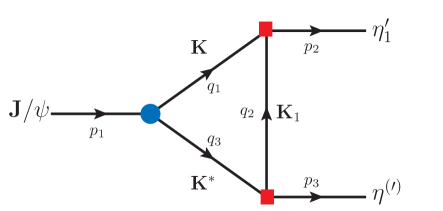
Figure 1: Rescattering decays.
In this section, we analyze the
decay in the molecular model. Its triangle-rescattering process, as depicted in
Fig. 1, can be separated into three parts:,
, and .
where , , and are the coupling
constants of the octet term, the mass-breaking term, and the
electromagnetic-breaking term, and the phase angle between electromagnetic and
strong interaction, respectively.
The second part is . The corresponding Lagrangian term
is
(5)
and the amplitude is derived to be
(6)
where is the Euclidean Jacobi momentum and
are the coupling constants of the decays.
For the sake of calculation,
and . The correlation function
can be parameterized as a Gaussian form vertex
function Branz:2007xp; Chen:2015igx or a pole form vertex
function Giacosa:2007bn; Giacosa:2012de; Schneitzer:2014rsa:
(7)
with is the size parameter. In this paper, the Gaussian form will
cause the integration divergence and, alternatively, we choose the pole vertex
form correlation function. We determine the coupling constants between the
hadronic molecule and its components using the pole vertex form by the
consequence of the lln-Lehmann representation (see
Eqs. 22-27) and the triangle diagram can be calculate by the
′tHooft-Veltman technique tHooft:1978jhc (see Eq. II).
Note that using the Gaussian form is more common than the Pole form to
determine the coupling constant by the compositeness condition in an one loop
diagram Weinberg:1962hj. However, calculating triangle diagram with the
Gaussian form may have singularities, called anomalous
thresholds Ivanov:2003ge. A parameter has been
proposed Branz:2009cd to prejudge whether there are anomalous
thresholds. The parameter describes the triangle diagram in which
particle decay into and particles with , , and particles as
propagators. Take Fig. 1 for example,
and . Then,
is given by
(8)
with and .
There will be no anomalous thresholds if is always positive.111
This could happen when, for example, is a molecular state and the circumstance
is satisfied.
In this paper, the set of masses
make not always positive, implying divergence will happen if the
Gaussian form is used.
The third part is , whose Lagrangian term and
amplitude are written as
(9)
and
(10)
where
(11)
and
(12)
where (, ) are the parameters for coupling constants and (,
) are the mixing angles of (,
) Divotgey:2013jba.
Eventually, the amplitude of the triangle-rescattering process for the
decay is obtained by
(13)
where sums over all possible Feynman diagrams for
, , , and ,
and
is the monopole form factor Tornqvist:1993ng; Li:1996yn; Yu:2020vlt,
which can be adopted to represent the off-shell effect by exchanging
mesons and also plays the role of avoiding integration divergences. Besides,
and correspond to the momentum
flows in Fig. 1. In the general form, one can expresses the
amplitude as
(14)
To obtain , one needs to integrate
over the variables of the triangle loop in Eq. 13, which gives
(15)
The propagators of and are supposed to contain vector and tensor
structures, but contributions from the tensor structures will be zero due to
the term in Eq. 13. Hence, we only
consider the vector structures here. The vector four-point function is
written as
(16)
such that one obtains
(17)
with the linear combination of scalar point functions
As for the term , one can obtain
by replacing in Eqs. (17-II) with . Next,
one can derive by comparing
Eqs. 14 and 15 and defining :
(20)
At this point, all parameters relevant to
are given except
, which can be determined by a consequence of the
lln-Lehmann representation (see the discussion below).
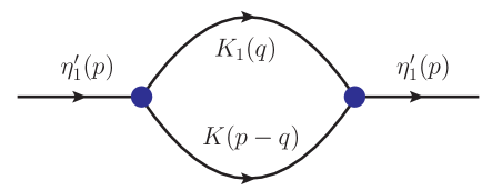
Figure 2: the one-loop correction to the propagator of .
Upon resummation of the one-loop contributions, as in Fig. 2, the
propagator of takes the form
(21)
The metric tensor term, , already provides enough information to
determine the coupling and the rest can be ignored
(denoted as […]). The spectral function of the state in the
lln-Lehmann representation can be obtained as the
imaginary part of the propagator Giacosa:2007bn; Giacosa:2012de:
(22)
and the normalization is required to be satisfied:
(23)
In the above equation, we define
(24)
and can give
(25)
where
(26)
and
(27)
The normalization of the spectral function of the ,
Eq. 23, causes a constraint in the lln-Lehmann
representation. With this constraint, the term in
Eq. II can be evaluated analytically with the ′tHooft-Veltman
technique.
More specifically, one can obtain an analytical expression for
by substituting Eqs. II-27 into Eq. 22.
After integrating out the momentum in Eq. 23, one can determine the
relationship between and , as shown in
Fig. 3. In this relationship, the masses of the relevant mesons are the
only input parameters.
Note that , , or itself possesses logarithmic
divergence. However, Eq. 25 doesn’t diverge because the divergence will
cancel by and .
III Numerical results and Discussions
In the numerical analysis, we adopt
, , =,
from Ref. Huang:2013wpa222Parameters
, , , and in SU(3) flavor symmetry theory
describe the to pseudoscalar-vector decays, e.g. ,
, and . They are extracted from fitting to
measured branching ratios.,
GeV, and from
Ref. Divotgey:2013jba.
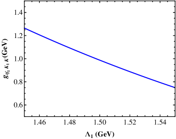
We can then fit GeV using
GeV Giacosa:2007bn; Giacosa:2012de; Schneitzer:2014rsa
and Eqs. 22-27. The choice of are typical in hadronic
theories. Figure 3 shows the coupling constant
related to . Empirically, we are
allowed to use GeV, which is not sensitive for the
branching ratio of because the
triangle Feynman diagrams to calculate
is convergent even without
the monopole form factor. As a consequence, we obtain
(28)
Approximately, we present the resonant branching fractions as
The uncertainty is evaluated by repeating the calculation after varying the
parameters according to their uncertainties. The uncertainty associated with
dominates. The larger yields the lower predicted
branching fractions, but when is set to be in the typical region,
the predicted branching fractions remains being of .
Figure 3: The coupling constant related to the
parameter .
IV Conclusions
The C-parity partner of , called , is a peculiar
prophecy in the molecular model. Confirming the existence of the
will be a critical support of the molecular model and helps
to pin down the nature of .
On the other side, the absence of would correspond to a
falsification of the molecular approach.
We have studied the rescattering decays
. In the triangle loop,
and transform as and by exchanging
, respectively. We have proposed the
decay as a candidate decay to search for the exotic state.
In particular, we have predicted
and
in the molecular model.
The BESIII collaboration has collected about 10 billion events at
GeV and can reach the sensitivity of -
level for branching fractions of decays. Our proposal is shown to be
accessible by the BESIII experiment.
ACKNOWLEDGMENTS
We would like to thank Dr. Zhi Yang, Xu-Chang Zheng, and Rui-Yu Zhou for useful discussions.
YY was supported in part by National Natural Science Foundation of China (NSFC) under Contracts No. 11905023, No. 12047564 and No. 12147102, the Natural Science Foundation of Chongqing (CQCSTC) under Contracts No. cstc2020jcyj-msxmX0555 and the Science and Technology Research Program of Chongqing Municipal Education Commission under Contracts No. KJQN202200605 and No. KJQN202200621; BCK was supported in part by NSFC under Contracts No. 11875054 and No. 12192263 and Joint Large-Scale Scientific Facility Fund of the NSFC and the Chinese Academy of Sciences under Contracts No. U2032104; JWZ was supported in part by NSFC under Contracts No. 12275036, CQCSTC under Contracts No. cstc2021jcyj-msxmX0681 and the Science and Technology Research Program of Chongqing Municipal Education Commission under Contracts No. KJQN202001541.