Kepler and TESS Observations of PG 1159-035

Abstract

PG 1159-035 is the prototype of the DOV hot pre-white dwarf pulsators. It was observed during the Kepler satellite K2 mission for 69 days in 59 s cadence mode and by the TESS satellite for 25 days in 20 s cadence mode. We present a detailed asteroseismic analysis of those data. We identify a total of 107 frequencies representing 32 $\ell=1$ modes, 27 frequencies representing 12 $\ell=2$ modes, and 8 combination frequencies. The combination frequencies and the modes with very high k values represent new detections. The multiplet structure reveals an average splitting of $4.0\pm 0.4\ \mu$Hz for $\ell$=1 and $6.8\pm 0.2\ \mu$Hz for $\ell=2$, indicating a rotation period of $1.4\pm 0.1$ days in the region of period formation. In the Fourier transform of the light curve, we find a significant peak at $8.904\pm 0.003\ \mu$Hz suggesting a surface rotation period of $1.299\pm 0.002$ days. We also present evidence that the observed periods change on timescales shorter than those predicted by current evolutionary models. Our asteroseismic analysis finds an average period spacing for $\ell=1$ of $21.28\pm 0.02$ s. The $\ell=2$ modes have a mean spacing of $12.97\pm 0.4$ s. We performed a detailed asteroseismic fit by comparing the observed periods with those of evolutionary models. The best fit model has $T_{\mathrm{eff}}=129\,600\pm 11\,100$ K, $M_{*}=0.565\pm 0.024M_{\odot}$, and $\log g=7.41^{+0.38}_{-0.54}$, within the uncertainties of the spectroscopic determinations. We argue for future improvements in the current models, e.g., on the overshooting in the He-burning stage, as the best-fit model does not predict excitation for all the pulsations detected in PG 1159-035.

1 Introduction

White dwarf (WD) stars are the evolutionary end point of all stars born with masses up to $\simeq 10.5~{}M_{\odot}$, which correspond to more than 98% of all stars (e.g. Lauffer et al., 2018). The effective temperature of WDs ranges from $T_{\mathrm{eff}}\simeq 200\,000~{}$ K to around $4500$ K, and masses from $\simeq 0.15~{}\mathrm{to}~{}\simeq 1.36~{}M_{\odot}$.

PG 1159-035 is the prototype of the hot WD spectroscopic class called PG 1159, as well as the GW Vir class of pulsating variable stars (PG 1159-035 = GW Vir = DOV) (McGraw et al., 1979; Córsico et al., 2019). The PG 1159 spectroscopic class is characterized by a strong H deficiency and high-excitation He II, C IV, O VI and N V lines (e.g. Werner et al., 1989; Sowicka et al., 2021; Werner et al., 2022). These are among the hottest pulsating stars known.

The pulsation modes observed in WDs are nonradial $g$ (gravity) modes. Gravity acts as the restoring force on the displaced portions of mass, moving it mainly horizontally. These pulsations cause different temperature zones that oscillate at eigenfrequencies, restricted by the spherical symmetry of the star.

In asteroseismology, we describe a pulsation mode using a spherical harmonic basis with three integer quantum numbers: $k$, $\ell$ and $m$. The number $k$ is called the radial index and is the number of radial nodes, related to how “deep” a mode is located in the star. The larger the radial index of a mode, the more superficial is its main region of period formation. The number $\ell$ is called the spherical harmonic index and is related to the number of latitudinal hot and cold zones. Finally, the number $m$ is called the azimuthal index, and its absolute value is related to the arrangement of those zones on the stellar surface. The number $m$ assumes integer values from $-\ell$ to $+\ell$. Rotation of the star breaks the degeneracy of the pulsation modes with same $k$ and $\ell$ but different $m$, causing the modes to split into $2\ell+1$ components in the Fourier Transform (FT) of its light curve.

Due to geometrical cancellation, we expect to observe predominantly modes with $\ell=1$ and $\ell=2$ in WDs (Robinson et al., 1982). These modes should produce triplets and quintuplets in Fourier Transforms (FT) of light curves of rotating WDs. This expectation is supported by the work of Stahn et al. (2005). The authors make use of the wavelength dependent flux variations, or chromatic amplitudes, for modes with different $\ell$. They extracted the chromatic amplitudes from 20 orbits of $\it{HST-STIS}$ time resolved spectra of PG 1159-035 between 1100 Å and 1750 Å. Comparing the results to models, they concluded that the most prominent pulsation mode at 516 s matches $\ell=1$ or $\ell=2$ modes only.

2 Previous datasets

PG 1159-035 has been observed by different ground-based telescopes since 1979 (Table 1). The ground-based data consist primarily of photometric observations obtained with CCDs and photomultiplier tubes. The Whole Earth Telescope (WET) runs in 1989, 1993, and 2002 were multi-site international campaigns dedicated to achieving 24 h coverage (Winget et al., 1991). In 2016 and 2021, this important star was continuously observed by space-based telescopes, enabling unprecedented quality data. Table 1 is a journal of the main observational campaigns since 1983. This table shows that, although the previous campaigns have comparable — or even longer — total lengths, the K2 data (2016) is by far the one with the most dense observations, followed by the TESS data (2021).

Year	Telescopes	Length	On star	Spectral
		(days)	(days)	resolution ($\mu$Hz)
1983	McDonald, SAAOa	96.0	2.7	0.12
1985	McDonald, SAAOa	64.6	2.0	0.18
1989	WETb	12.1	9.5	0.96
1993	WETc	16.9	14.4	0.68
2002	WETd	14.8	4.8	0.78
2016	Kepler	69.1	54.5	0.17
2021	TESS	24.9	22.0	0.46

^a Winget et al. (1985); ^b Winget et al. (1991); ^c Bruvold (1993);
^d Costa et al. (2003)

Table 1: Main observational campaigns of PG 1159-035 between 1983 and 2021.

Figure 1 shows the Fourier transform (FT) for each annual observation of PG 1159-035, in the range of the higher amplitude peaks (1700-2300 $\mu$Hz, or roughly $435-590$ s), and their respective spectral window on the right side.

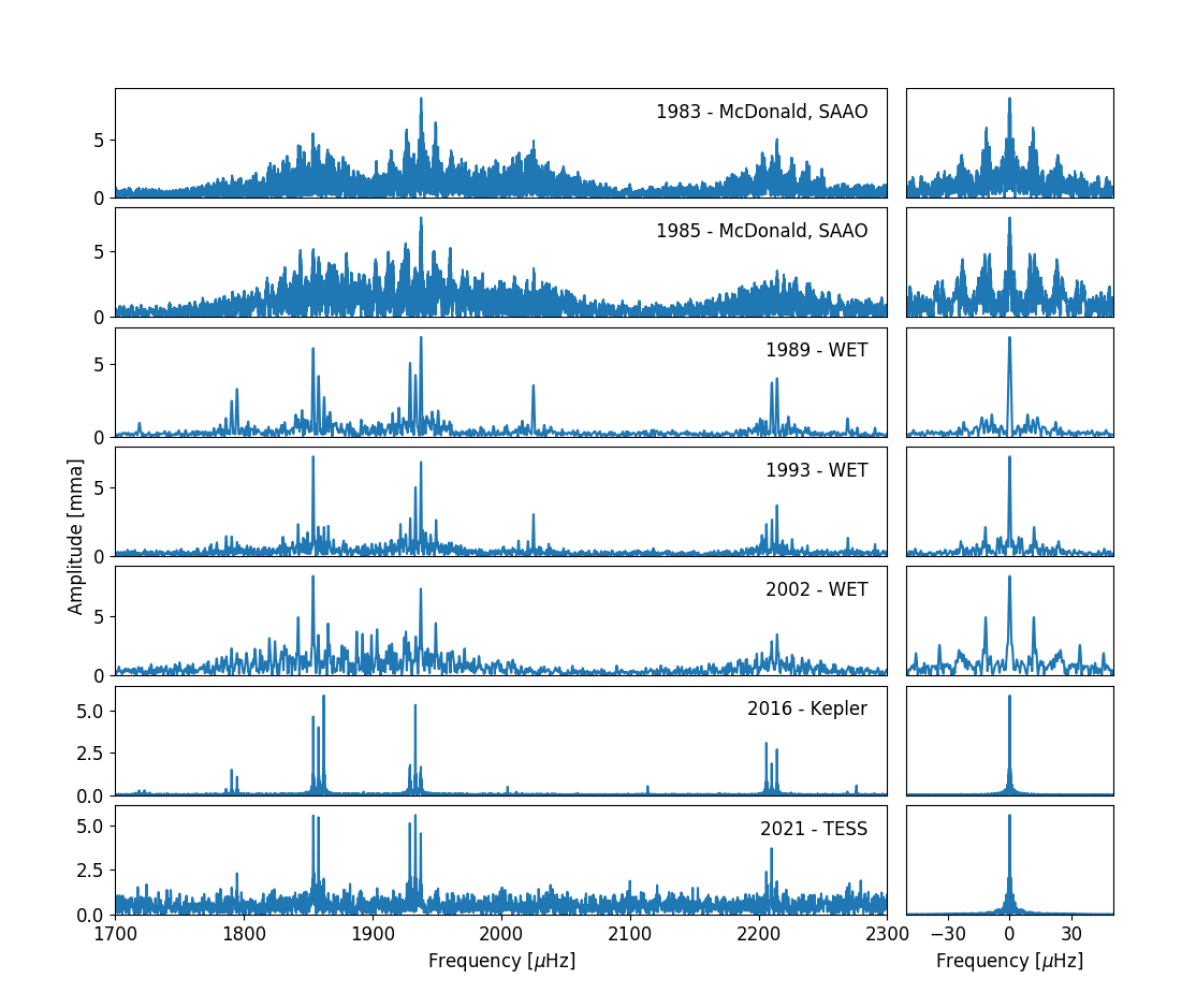
Figure 1: Fourier transform of PG 1159-035 of the years of 1983, 1985, 1989, 1993, 2002, 2016 and 2021, from 1700 to 2300 $\mu\mathrm{Hz}$. Their respective spectral windows are shown on the right side. Frequencies are in $\mu\mathrm{Hz}$ and amplitude units use 1 mma = 1/1.086 mmag = 1 ppt = 0.1%, see e.g. Bognar & Sodor (2016).

As shown in this figure, the K2 data spectral window has the sharpest structure, allowing the triplets to appear more clearly in the FT. The TESS data spectral window also has very little structure, but the TESS data signal-to-noise ratio is limited by the small size of the telescope and the redder bandpass. PG 1159-035 is very blue ($T_{\mathrm{eff}}\approx 140,000$K) and faint ($m_{v}=15.04$). The higher noise found in the TESS data hinders the detection of the numerous low amplitude frequencies found in the K2 data.

3 K2 and TESS Observational Data

After a failure of the second reaction wheel controlling the pointing of the Kepler spacecraft, observations along the ecliptic plane were enabled by the K2 mission (Howell et al., 2014). K2 observed PG 1159-035 (EPIC 201214472) between July and September 2016 during Campaign 10. We downloaded the target pixel files (TPFs) in short cadence (58.85s) from the Barbara A. Mikulski Archive for Space Telescopes (MAST), and used the Lightkurve package (Lightkurve Collaboration et al., 2018) to extract photometry from the TPFs. As K2 suffers a $\sim 6.5$ hr thruster firing to compensate for the solar pressure variation for fine pointing, we subsequently used the KEPSFF routine (Vanderburg & Johnson, 2014) to correct the systematic photometric variation that is induced by the low-frequency motion of the target on the CCD module. A series of apertures of different pixel sizes were tested on the TPF to optimize the photometry. We finally chose a fixed 30-pixel aperture to extract our light curve. After extracting the photometry, we fit a third-order polynomial and sigma clipped the light curve to 4.5$\sigma$ in order to detrend the light curve and to clip the outliers. We also subtracted the known electronic spurious frequencies and their harmonics (Van Cleve et al., 2016). The K2 data starts at Barycentric Julian Dates in Barycentric Dynamical Time BJD_TDB=2457582.5799677 and extends 69.14 days, with 58.8 s cadence.

The TESS data were collected in 2021 December during Sector 46 with the spacecraft’s fastest 20 s cadence. The data were downloaded from the MAST Portal and used PDCSAP simple aperture fluxes, after removal of 5$\sigma$ outliers. PG 1159-035 is TIC 35062562 in the TESS Target Input Catalog.

4 Detection of pulsation periods

We used the Period04 Fourier analysis software (Lenz & Breger, 2004) to detect the pulsation frequencies and subtract their respective sinusoids from the light curves of K2 (pre-whitening). We estimated the false-alarm-probability (fap) of 1/1000 by randomizing the input 1000 times, as the data consists of multiple coherent frequencies.

After the subtraction of each peak found in the Fourier Transform (FT) directly from the light curve, we calculated the detection limit of the residual light curve. We repeated this process until the highest amplitude peak had a false alarm probability larger than $1/1000$.

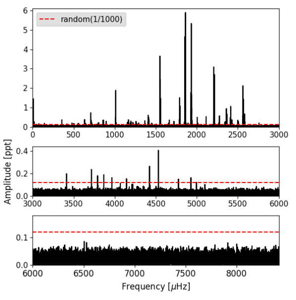
Figure 2: Fourier Transform of the original K2 light curve of PG 1159-035. The red dashed line indicates the false alarm probability fap(1/1000)=0.119 mma we obtained randomizing the input times 1000 times. Frequencies are in $\mu\mathrm{Hz}$ and amplitudes in $ppt$

.

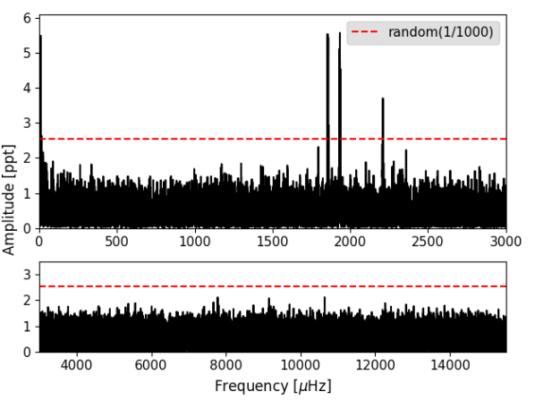
Figure 3: Fourier Transform of the original TESS light curve of PG 1159-035. The red dashed line indicates the false alarm probability fap(1/1000)= 2.537 mma we obtained randomizing the input times 1000 times.

Tables 2 and 3 list the $\ell=1$ and $\ell=2$ frequencies detected in the K2, and Table 4 in the TESS data sets. The values for the periods given in the tables were determined by non-linear simultaneous multisinusoidal least-squares fit and their uncertainties by Monte Carlo simulation, as in Costa et al. (2008).

5 Mode coherence

Asteroseismic analysis is based on the detected mode properties. The basic underlying assumption is that the frequencies and amplitudes of the pulsations modes are stable on a much longer baseline than that of the observations. Changes in stellar structure do affect the amplitude and frequency of pulsation modes. The Fourier transforms of PG 1159-035 from different epochs show different mode frequencies and amplitudes (Figures 1 and 4), indicating that its pulsation modes are not strictly coherent on time scales of months or years.

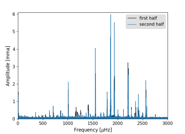
Figure 4: Fourier transform of first half and second half of the K2 data, showing amplitude changes during the 69 d observations, especially for peaks between 1100 and 1400 $\mu$Hz.

The intrinsic width of a mode in the power spectra is inversely related with its lifetime. A coherent mode appears in the power spectra as a single peak with a width dictated by the length of the observations. Such a peak has a lifetime considerably longer than the time span of the data set. On the other hand, if the observational campaign is lengthy enough to observe them, an incoherent mode with a short lifetime appears in the power spectra as a multitude of closely spaced peaks (e.g. Basu & Chaplin, 2017).

Motivated by the results presented in Hermes et al. (2017b) about the dichotomy of mode widths for ZZ Ceti (DAV) stars, we fitted Lorentzian envelopes by least-squares to every set of peaks detected in the K2 data power spectrum, as in Bell et al. (2015). We used the highest-amplitude peak within each set of peaks as an initial guess for the central frequency and Lorentzian height. For the half-width at half-maximum (HWHM), we take twice the frequency resolution as an initial guess.

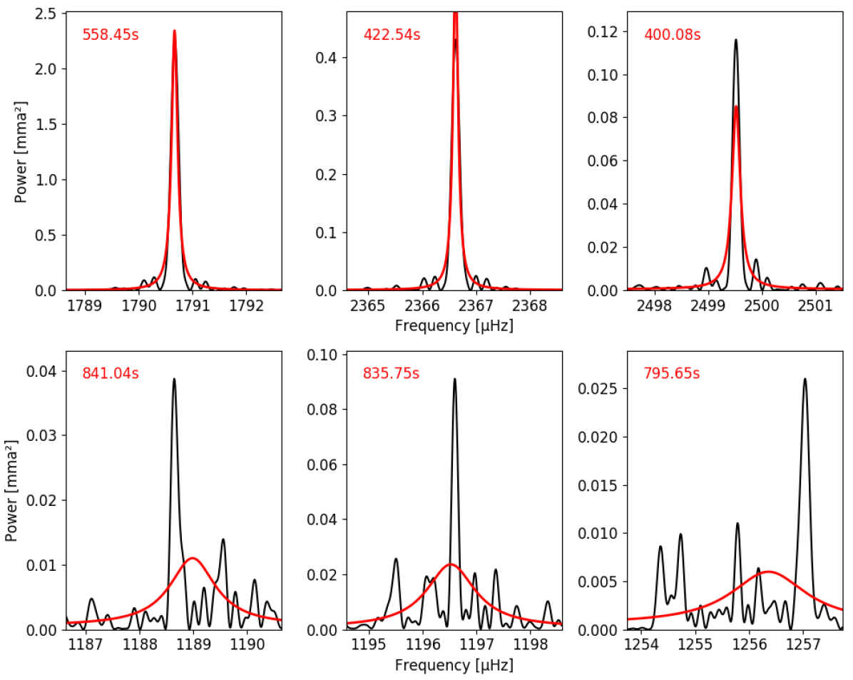
Figure 5: Detailed portions of the K2 data power spectrum of PG 1159-035 illustrating some Lorentzian fits as red lines. The frequency is in $\mu$Hz and the power is in units of mma² ($1\ \mathrm{mma}=1\ \mathrm{ppt}$). All plots have the same frequency range of $4\,\mu$Hz, but different power ranges. In the top panel, we show some modes whose HWHM are very close to the frequency resolution and, in the bottom panel, we show those modes with the widest HWHM.

We used the Lorentzian fits to determine the independent frequencies: we assume that all peaks covered by the Lorentzian represent the same mode. And, for modes whose Lorentzian fit covers more than one peak, we defined its HWHM as a width range. For these modes, the uncertainties are unreliable, once they are not coherent over the data set. The frequency and amplitude of the non-coherent modes are, respectively, the central frequency and height of the fitted Lorentzian.

Some Lorentzian fits are very close to the shape of a single peak, but others cover a few peaks, as illustrated by Figure 5. To determine if the distribution of Lorentzian widths is random or presents some pattern, we plot the HWHM of Lorentzian fits against period. Figure 6 shows that the largest values of HWHM are in the period range of $\approx 400-1000$ s. The highest points correspond to three $\ell=1$ modes: $k=33$, 34 and 35 . This is comparable with the results on DAVs of Hermes et al. (2017b), who found that the largest values of HWHM are in the period range $800-1400$ s. We note the largest values of HWHM in their sample of DAVs are several times larger than those seen in the PG 1159-035 data. Montgomery et al. (2020) showed that the dichotomy in HWHM values for the DAVs could be explained by changes in the surface convection zone during pulsation. These changes alter the reflection condition for modes, making these modes less coherent.

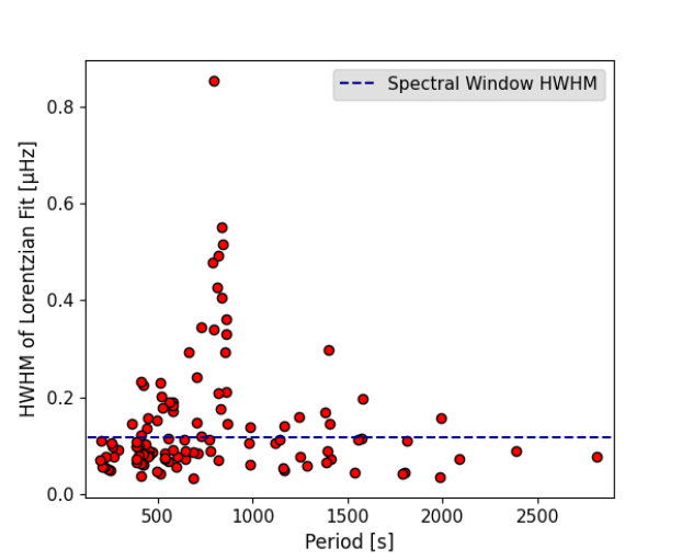
Figure 6: Half-width at half-maximum (HWHM) of Lorentzian fit to the significant peaks in the Fourier Transform of PG 1159-035 in $\mu\mathrm{Hz}$ vs. their periods in seconds. The horizontal blue dashed indicates the spectral window HWHM of the K2 data.

Models of PG 1159 stars generally show neither surface nor sub-surface convection zones (e.g. Miller Bertolami & Althaus, 2006; Córsico & Althaus, 2006), so the mechanism of Montgomery et al. (2020) is not expected to lead to a lack of mode coherence for this case. It is possible that other nonlinear effects come in to play near the outer turning point of some modes, which leads to a lack of coherent reflection. As an example, the large amplitudes of some modes could lead to a Kelvin-Helmholtz instability (shear instability) in the outer layers of the star, leading to energy loss and inconsistent reflection of the modes. Nonlinear mode coupling on similar timescales has been observed in two pulsating DBVs, by Kepler et al. (2003) and Zong et al. (2016), consistent with the amplitude equations of Goupil & Buchler (1994) and Buchler et al. (1995).

6 The period spacing and mode identification

6.1 K2 data

According to pulsation theory, the period spacing $\Delta\Pi_{l}$ between two g-modes with the same $\ell$, $m=0$, and consecutive $k$ is constant for a homogeneous model in the asymptotic limit ($k\gg\ell$). We can write the following general equation:

$$\Pi_{\ell,k}=\Pi_{\ell,0}+k\Delta\Pi_{\ell}$$ (1)

where $\Pi_{\ell,k}$ is the period of a $(k,\ell,m=0)$ mode, and $\Pi_{\ell,0}$ is the period of the $k=0$ mode (Tassoul, 1980; Winget et al., 1991).

To identify sequences of consecutive k modes for different $\ell$ values, we need initial guesses for the constants of the equation above. We used the Kolmogorov-Smirnov test (type: KP - Kuiper statistic) to get an initial value for the period spacing $\Delta\Pi_{1}$ and $\Delta\Pi_{2}$. Figure 7 shows the K-S test applied to our list of independent frequencies. We identified six significant peaks in the test: $\Delta\Pi_{\mathrm{1}}=21.23$ s, $\Delta\Pi_{\mathrm{2}}=12.97$ s and two multiples of each one. The $\Delta\Pi_{\mathrm{1}}$ peak is significantly stronger than its multiples. This is not true to $\Delta\Pi_{\mathrm{2}}$, which has a significance $\log Q$ value similar to its multiples. This may result from the smaller number of $\ell=2$ frequencies observed compared to the sample of $\ell=1$ frequencies.

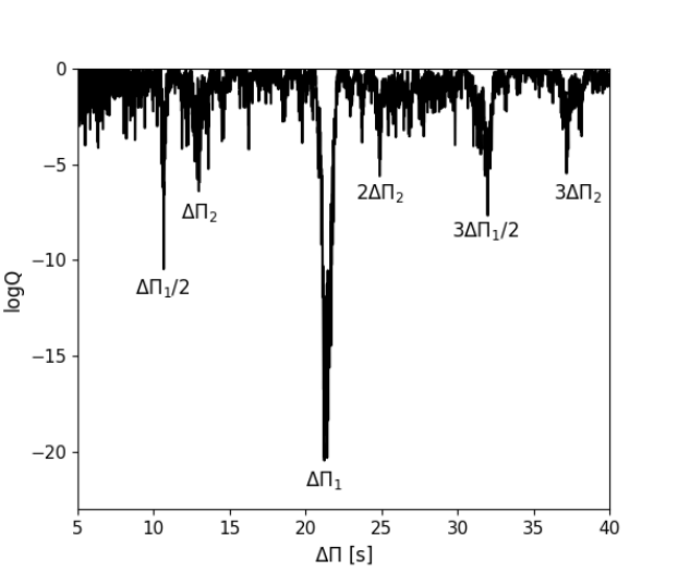
Figure 7: K-S test applied to our list of independent frequencies. There are six significant peaks: two of them correspond to $\Delta\Pi_{\mathrm{1}}$ and $\Delta\Pi_{\mathrm{2}}$ values, and the others are multiples of these.

We would also like to place constraints on the values of $\bf\Pi_{\ell=1,0}$ and $\bf\Pi_{\ell=2,0}$. For slow rotation in the absence of a magnetic field, the components of a split mode are equally spaced in frequency by a constant $\delta\nu_{\ell}$. To identify multiplets in the set of frequencies observed, it is important to estimate $\delta\nu_{\ell}$. As initial guesses, we took the values obtained by Winget et al. (1991), $\delta\nu_{\ell=1}=4.22$ and $\delta\nu_{\ell=2}=6.92$. Further, using the results of Winget et al. (1991) to assume that the triplet at $517$ s is the $k=20\pm 2$, $\ell=1$ mode, we find from equation $(1)$: $\Pi_{0,\ell=1}=92.6$ s. Using the results of Costa et al. (2008) to assume that the quintuplet of $387$ s is the $k=27\pm 2,\ \ell=2$ mode, we obtain $\Pi_{0,\ell=2}=37.98$ s.

Taking these values to classify the K2 frequencies in the range of $300-3000$ $\mu\mathrm{Hz}$, we identified $32$ $\ell=1$ independent modes (Table 2) and $12$ $\ell=2$ independent modes (Table 3). The fourteen $\ell=1$ modes with the largest values of $k$ are out of the frequency range analyzed by Costa et al. (2008), and the $k=61,\ell=2$ mode was not detected in their data.

$k\pm 2$	m	Period	Frequency	Amplitude	$k\pm 2$	m	Period	Frequency	Amplitude
		[s]	[$\mu$Hz]	[mma]			[s]	[$\mu$Hz]	[mma]
14	+1	$386.8818\pm 0.0013$	$2584.769\pm 0.008$	$0.26\pm 0.02$	35*	+1	$835.75\pm 0.38$	$1196.53\pm 0.55$	$0.15$
14	0	$387.5045\pm 0.0013$	$2580.615\pm 0.009$	$0.25\pm 0.02$	35*	0	$838.50\pm 0.29$	$1192.61\ \pm 0.41$	$0.13$
14	-1				35*	-1	$841.05\pm 0.36$	$1188.99\pm 0.52$	$0.10$
17	+1	$451.6086\pm 0.0002$	$2214.307\pm 0.001$	$2.70\pm 0.02$	42	+1	$981.7223\pm 0.0100$	$1018.618\pm 0.010$	$0.21\pm 0.02$
17	0	$452.4465\pm 0.0002$	$2210.206\pm 0.001$	$1.87\pm 0.02$	42	0	$985.6528\pm 0.0093$	$1014.556\pm 0.010$	$0.23\pm 0.02$
17	-1	$453.2911\pm 0.0001$	$2206.088\pm 0.001$	$3.14\pm 0.02$	42	-1	$988.4763\pm 0.0011$	$1011.658\pm 0.001$	$1.88\pm 0.02$
18	+1				48	+1
18	0	$473.0622\pm 0.0009$	$2113.887\pm 0.004$	$0.52\pm 0.02$	48	0	$1116.0179\pm 0.0096$	$896.043\pm 0.008$	$0.29\pm 0.02$
18	-1				48	-1
20*	+1	$516.10\pm 0.06$	$1937.59\ \pm 0.23$	$1.28$	50	+1	$1159.3618\pm 0.0085$	$862.543\pm 0.006$	$0.35\pm 0.02$
20	0	$517.2150\pm 0.0001$	$1933.432\pm 0.001$	$5.34\pm 0.02$	50	0	$1164.8798\pm 0.0107$	$858.458\pm 0.008$	$0.28\pm 0.02$
20*	-1	$518.34\pm 0.05$	$1929.24\ \pm 0.20$	$1.46$	50	-1	$1168.7091\pm 0.0088$	$855.645\pm 0.006$	$0.34\pm 0.02$
21	+1	$536.9727\pm 0.0001$	$1862.292\pm 0.001$	$5.92\pm 0.02$	54	+1	$1242.0046\pm 0.0150$	$805.150\pm 0.010$	$0.23\pm 0.02$
21	0	$538.1587\pm 0.0002$	$1858.188\pm 0.001$	$4.08\pm 0.02$	54	0	$1246.2601\pm 0.0216$	$802.401\pm 0.014$	$0.16\pm 0.02$
21	-1	$539.3473\pm 0.0001$	$1854.093\pm 0.001$	$4.74\pm 0.02$	54	-1	$1252.6274\pm 0.0178$	$798.322\pm 0.011$	$0.19\pm 0.02$
22	+1	$557.1217\pm 0.0006$	$1794.940\pm 0.002$	$1.14\pm 0.02$	56	+1
22	0	$558.4483\pm 0.0004$	$1790.676\pm 0.001$	$1.53\pm 0.02$	56	0	$1284.5235\pm 0.0254$	$778.499\pm 0.015$	$0.14\pm 0.02$
22*	-1	$559.78\pm 0.06$	$1786.42\pm 0.19$	$0.27$	56	-1
23*	+1	$579.07\pm 0.06$	$1726.90\pm 0.18$	$0.11$	61	+1	$1379.2645\pm 0.0309$	$725.024\pm 0.016$	$0.14\pm 0.02$
23*	0	$580.38\pm 0.06$	$1723.00\pm 0.19$	$0.18$	61	0	$1387.0651\pm 0.0210$	$720.947\pm 0.011$	$0.20\pm 0.02$
23*	-1	$581.78\pm 0.06$	$1718.85\pm 0.17$	$0.20$	61	-1	$1392.6642\pm 0.0299$	$718.048\pm 0.015$	$0.14\pm 0.02$
24	+1	$600.6547\pm 0.0023$	$1664.850\pm 0.006$	$0.34\pm 0.02$	62*	+1	$1398.74\pm 0.58$	$714.93\pm 0.30$	$0.16$
24	0				62	0	$1406.5058\pm 0.0122$	$710.982\pm 0.006$	$0.36\pm 0.02$
24	-1	$604.0409\pm 0.0041$	$1655.517\pm 0.011$	$0.20\pm 0.02$	62	-1	$1412.1701\pm 0.0000$	$708.130$	$0.72\pm 0.02$
26	+1	$641.5557\pm 0.0006$	$1558.711\pm 0.001$	$1.49\pm 0.02$	68	+1
26	0	$643.2361\pm 0.0004$	$1554.639\pm 0.001$	$2.54\pm 0.02$	68	0	$1539.0279\pm 0.0342$	$649.761\pm 0.014$	$0.15\pm 0.02$
26	-1	$644.9279\pm 0.0002$	$1550.561\pm 0.001$	$3.68\pm 0.02$	68	-1
27	+1				69	+1
27	0	$664.1985\pm 0.0068$	$1505.574\pm 0.015$	$0.14\pm 0.02$	69	0	$1555.7422\pm 0.0335$	$642.780\pm 0.014$	$0.16\pm 0.02$
27	-1				69	-1
28	+1	$685.7765\pm 0.0067$	$1458.201\pm 0.014$	$0.15\pm 0.02$	70	+1
28	0				70*	0	$1572.9948\pm 0.0000$	$635.730$	$0.37\pm 0.02$
28	-1	$689.6951\pm 0.0056$	$1449.916\pm 0.012$	$0.19\pm 0.02$	70	-1	$1589.91\pm 0.49$	$632.95\pm 0.20$	$0.29$
29*	+1	$706.08\pm 0.12$	$1416.27\pm 0.24$	$0.27$	80	+1	$1788.9168\pm 0.0392$	$558.998\pm 0.012$	$0.18\pm 0.02$
29	0	$708.1235\pm 0.0021$	$1412.183\pm 0.004$	$0.51\pm 0.02$	80	0	$1802.1048\pm 0.0437$	$554.907\pm 0.013$	$0.16\pm 0.02$
29	-1	$710.3398\pm 0.0018$	$1407.777\pm 0.004$	$0.61\pm 0.02$	80	-1	$1811.2402\pm 0.0400$	$552.108\pm 0.012$	$0.18\pm 0.02$
30	+1				89	+1
30*	0	$729.60\pm 0.18$	$1370.61\pm 0.35$	$0.11$	89	0	$1982.7768\pm 0.0504$	$504.343\pm 0.013$	$0.17\pm 0.02$
30	-1	$731.6054\pm 0.0037$	$1366.857\pm 0.007$	$0.32\pm 0.02$	89	-1	$1993.56\pm 0.07$	$501.615\pm 0.017$	$0.13\pm 0.02$
32	+1				90	+1
32	0	$773.7070\pm 0.0066$	$1292.479\pm 0.011$	$0.20\pm 0.02$	90	0	$2010.0490\pm 0.0569$	$497.500\pm 0.014$	$0.16\pm 0.02$
32	-1	$776.0878\pm 0.0078$	$1288.514\pm 0.013$	$0.17\pm 0.02$	90	-1	$2021.2441\pm 0.0613$	$494.745\pm 0.015$	$0.15\pm 0.02$
33*	+1	$791.56\pm 0.30$	$1263.33\ \pm 0.48$	$0.16$	94	+1
33*	0	$793.89\pm 0.21$	$1259.62\pm 0.34$	$0.20$	94	0	$2084.6910\pm 0.0501$	$479.687\pm 0.012$	$0.19\pm 0.02$
33*	-1	$795.5298\pm 0.0092$	$1257.024\pm 0.015$	$0.15\pm 0.02$	94	-1
34*	+1	$813.77\pm 0.28$	$1228.85\pm 0.43$	$0.08$	128	+1
34*	0	$816.68\pm 0.14$	$1224.46\pm 0.21$	$0.13$	128	0	$2807.9405\pm 0.0463$	$356.133\pm 0.006$	$0.37\pm 0.02$
34*	-1	$819.02\pm 0.33$	$1220.98\pm 0.49$	$0.15$	128	-1

Table 2: Identified $\ell=1$ pulsation modes in K2 data. The frequencies with an ‘*’ after the k number are not coherent during observations, and their parameters are the values referring to Lorentzian fits.

$k\pm 2$	m	Period	Frequency	Amplitude	$k\pm 2$	m	Period	Frequency	Amplitude
		[s]	[$\mu$Hz]	[mma]			[s]	[$\mu$Hz]	[mma]
25	+2				32	+2
25	+1				32	+1
25	0	$362.5385\pm 0.0014$	$2758.328\pm 0.011$	$0.21\pm 0.02$	32	0	$449.3623\pm 0.0032$	$2225.376\pm 0.016$	$0.14\pm 0.02$
25	-1				32	-1
25	-2				32	-2
27	+2				36	+2
27	+1	$387.1166\pm 0.0005$	$2583.201\pm 0.003$	$0.65\pm 0.02$	36	+1	$497.0416\pm 0.0028$	$2011.904\pm 0.011$	$0.19\pm 0.02$
27	0				36	0	$498.7392\pm 0.0011$	$2005.056\pm 0.004$	$0.50\pm 0.02$
27	-1	$389.2308\pm 0.0002$	$2569.170\pm 0.002$	$1.45\pm 0.02$	36	-1
27	-2	$390.2865\pm 0.0002$	$2562.220\pm 0.001$	$2.12\pm 0.02$	36	-2
28	+2				38	+2
28	+1	$398.9886\pm 0.0013$	$2506.337\pm 0.008$	$0.28\pm 0.02$	38	+1
28	0	$400.0776\pm 0.0010$	$2499.515\pm 0.006$	$0.34\pm 0.02$	38*	0	$528.21\pm 0.05$	$1893.20\ \pm 0.18$	$0.11$
28	-1				38	-1
28	-2				38	-2
29	+2	$410.8695\pm 0.0025$	$2433.863\pm 0.015$	$0.15\pm 0.02$	61	+2
29*	+1	$412.04\pm 0.04$	$2426.97\pm 0.23$	$0.24$	61	+1
29	0				61	0
29	-1	$414.4032\pm 0.0004$	$2413.109\pm 0.002$	$1.05\pm 0.02$	61*	-1	$833.58\pm 0.12$	$1199.65\pm 0.18$	$0.17$
29	-2	$415.5943\pm 0.0008$	$2406.193\pm 0.005$	$0.48\pm 0.02$	61	-2
30	+2	$422.5439\pm 0.0006$	$2366.618\pm 0.003$	$0.65\pm 0.02$	63	+2
30	+1	$423.7669\pm 0.0004$	$2359.788\pm 0.002$	$0.94\pm 0.02$	63	+1
30	0				63*	0	$856.55\pm 0.21$	$1167.47\pm 0.29$	$0.28$
30*	-1	$426.26\pm 0.04$	$2346.01\pm 0.22$	$0.19$	63*	-1	$861.00\pm 0.25$	$1161.44\pm 0.33$	$0.11$
30	-2	$427.4673\pm 0.0017$	$2339.360\pm 0.009$	$0.23\pm 0.02$	63	-2	$866.2231\pm 0.0081$	$1154.437\pm 0.011$	$0.20\pm 0.02$
31	+2				64*	+2	$859.36\pm 0.27$	$1163.66\pm 0.36$	$0.14$
31	+1				64*	+1	$864.21\pm 0.16$	$1157.13\pm 0.21$	$0.20$
31	0				64	0
31	-1	$439.3573\pm 0.0007$	$2276.052\pm 0.004$	$0.57\pm 0.02$	64	-1
31	-2	$440.7055\pm 0.0021$	$2269.089\pm 0.011$	$0.20\pm 0.02$	64	-2

Table 3: Identified $\ell=2$ pulsation modes in K2 data. The frequencies with an ‘*’ after the k number are not coherent during observations, and their parameters are the values referring to Lorentzian fits.

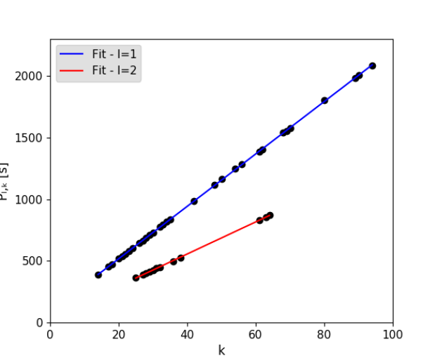
Figure 8: Observed periods sequences for $\ell=1$ (blue line) and $\ell=2$ (red line) modes from K2 data.

After identifying the modes, we were able to use their observational values to improve our constants. We plotted the periods vs. their assigned $k$ value to the $\ell=1$ and $\ell=2$ modes, as shown in Figure 8. So, fitting a line according to Equation $(1)$, we obtain:

$$\Delta\Pi_{\textit{1}}=21.28\pm 0.02~{}\mathrm{s}\quad\mathrm{and}\quad\Delta\Pi_{\textit{2}}=13.02\pm 0.04~{}\mathrm{s}$$ (2)

These values are very similar to the ones found by Costa et al. (2008): $\Delta\Pi_{\textit{1}}=21.43\pm 0.03~{}\mathrm{s}$ and $\Delta\Pi_{\textit{2}}=12.38\pm 0.01~{}\mathrm{s}$. The ratio between the period spacings we obtained is:

$$\frac{\Delta\Pi_{\textit{1}}}{\Delta\Pi_{\textit{2}}}=1.634\pm 0.005$$ (3)

that is, 94% of $\sqrt{3}$, the value expected by asymptotic pulsation theory.

6.2 TESS data

In Fig. 1 we observe that TESS data is much noisier than K2 data. The higher noise levels make it impossible to detect low amplitude frequencies. We are unable to complete a deep analysis. Since we do not gain any new insights from the TESS data compared to the K2 data, we only consider the K2 data for the remainder of this manuscript.

$k\pm 2$	m	Period	Frequency	Amplitude
		[s]	[$\mu$Hz]	[mma]
17	1
17	0	$452.462\pm 0.006$	$2210.13\pm 0.03$	$3.7\pm 0.4$
17	-1	$453.307\pm 0.009$	$2206.01\pm 0.04$	$2.4\pm 0.4$
20	1	$516.107\pm 0.006$	$1937.58\pm 0.02$	$4.5\pm 0.4$
20	0	$517.211\pm 0.005$	$1933.45\pm 0.02$	$5.7\pm 0.4$
20	-1	$518.370\pm 0.005$	$1929.12\pm 0.02$	$5.2\pm 0.4$
21	1
21	0	$538.155\pm 0.006$	$1858.20\pm 0.02$	$5.5\pm 0.4$
21	-1	$539.333\pm 0.005$	$1854.14\pm 0.02$	$5.5\pm 0.4$

Table 4: Identified pulsation frequencies in TESS data.

7 Mode structure and Asymmetries

7.1 $\ell=1$ modes

The 32 $\ell=1$ modes identified in the K2 light curve are distributed in 8 singlets, 8 doublets, and 16 triplets. For the 24 modes with multiplet structure, we find 15 with approximately symmetric splitting of $\langle\delta\nu_{\rm rot,1}\rangle=(4.0\pm 0.4)~{}\mu$Hz. The remaining nine $\ell=1$ multiplets have a very similar asymmetric frequency structure, as shown in Figures 9 and 14. The asymmetric modes present a larger spacing average $\langle\delta\nu_{\rm rot,1}^{+}\rangle=(4.06\pm 0.05)~{}\mu$Hz and a smaller spacing average $\langle\delta\nu_{\rm rot,1}^{-}\rangle=(2.81\pm 0.06)~{}\mu$Hz. For the major asymmetric modes, the larger spacing is that between the $m=0$ and $m=1$ frequencies. The $k=54$ mode is an exception, with the larger spacing between the $m=-1$ and $m=0$ frequencies. Please note that the x-axis of the $k=54$ panel is inverted in Figure 9.

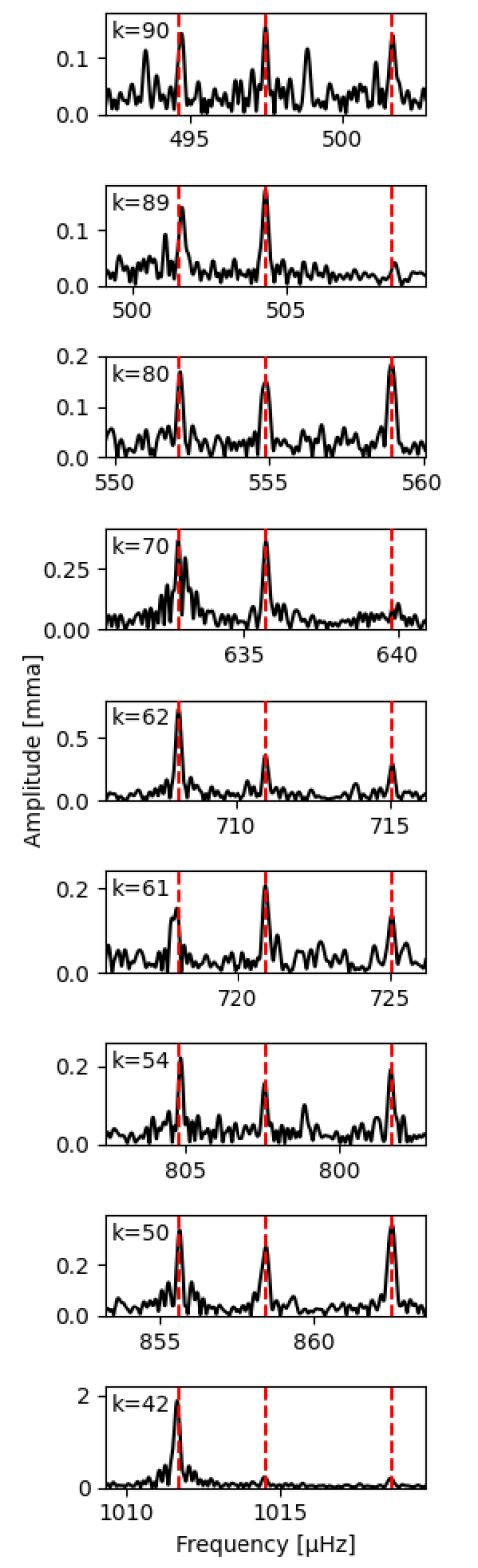
Figure 9: The panels show detailed portions of the K2 FT centered in the $m=0$ frequency of the asymmetric modes. The red dashed lines indicates the $\langle\delta\nu_{\mathrm{rot,1}}\rangle$ frequency spacing averages.

Figure 10 shows the asymmetry observed in $\ell=1$ modes in PG 1159$-$035 as a function of the radial node $k$. While the pulsations are global, each pulsation samples the star in slightly different ways. The lower k modes have outer turning points that are far below the stellar surface, so these modes preferentially sample the deeper interior. High k modes sample more of the outer layers. Figure 10 shows that the larger asymmetries are found in modes with larger values of k. This argues that the cause of the asymmetries, whether it be magnetic fields, differential rotation or some other symmetry-breaking agent, predominately influences the outer layers corresponding to $40\leq k\leq 80$ rather than in the inner zone corresponding to $k\leq 30$.

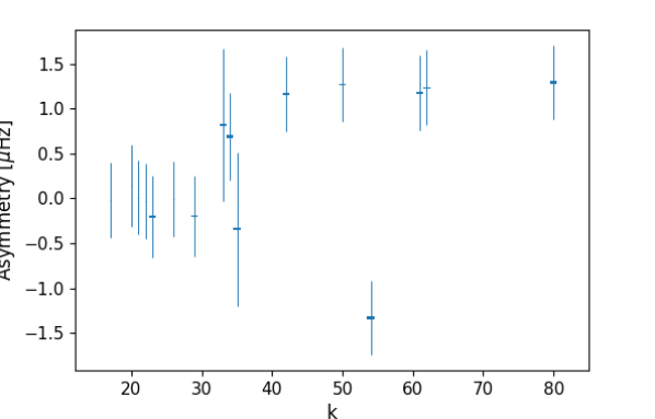
Figure 10: Asymmetry of the $\ell$ = 1 modes as a function of the radial node $k$. The height of the square markers correspond to the internal uncertainties calculated by MC Monte Carlo simulation. The error bars indicate the uncertainties obtained by the Lorentzian fit.

In the case of weak magnetic fields and slow ($\omega_{\mathrm{puls}}>\Omega_{\mathrm{rot}}$) uniform rotation, the observed frequency spacing depends on both the rotation period and the magnetic field of the star. Assuming that the pulsation axis, the rotation axis and the magnetic field are aligned, the frequency spacing can be approximated in first order by (e.g. Hansen et al., 1977; Jones et al., 1989; Gough & Thompson, 1990; Dintrans & Rieutord, 2000) :

$$\delta\nu\ \approx\ m(1-C)\Omega_{\mathrm{rot}}\ +\ m^{2}\bar{\gamma}B^{2}$$ (4)

where the Ledoux constant $C=C(k,\ell)$ is the uniform rotation coefficient (Ledoux, 1951), $\Omega_{\mathrm{rot}}$ is the rotational frequency, $\bar{\gamma}$ is a proportionality constant and $B$ is the magnetic field. Because of its dependence on $m^{2}$, the magnetic field term in equation 4 causes an asymmetric splitting about $m=0$ if combined with the rotational effect. Defining:

$$\mathrm{Asymmetry}(k,\ell)\approx\delta\nu(k,\ell,m=+1)+\delta\nu(k,\ell,m=-1)$$

$$\mathrm{Asymmetry}(k,\ell)\approx 2\bar{\gamma}B^{2}$$ (5)

with the asymmetry directly related with the square of the magnetic field.

From Figure 14, however, we can see that the exact morphology of the splitting does not follow the form of equation 4. While the $m=-1$ components are shifted to the right (toward the $m=0$ modes), the $m=+1$ components should also be shifted to the right, away from the $m=0$ modes. This is not observed. Thus, the simple model of uniform rotation plus a uniform magnetic field in which the magnetic and rotation axes are aligned cannot be valid. But if we assume differential rotation, as suggested by Figure 14, a lower rotational frequency in the period formation zone of the asymmetric modes plus an off-center magnetic field could explain Figure 10. Second order effects of rotation also can produce an asymmetry in multiplets, even for the slow rotators (Dziembowski & Goode, 1992).

However, it is important to point that all this discussion is based on the assumption that the quantum numbers $\it{k}$, $\ell$ and $m$ assigned to the frequencies lower than 1100 $\mu$Hz are correct. We have suggested a mode identification in Table 2 using the $\Pi_{\ell,k}$ model we have calculated in section 6.1. In the range of low frequencies, this model present a strong superposition of both $\ell=1$ and $\ell=2$ modes (see Figure 11), leading to other equally possible mode identification to these frequencies: the possibility that these sets of frequencies are not asymmetric $\ell=1$ modes but superposition of $\ell=1$ and $\ell=2$ modes, or nonlinear difference frequencies.

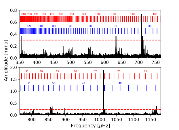
Figure 11: K2 data FT in the range of asymmetric modes. Vertical blue lines indicate the component m=0 of the $\ell=1$ model calculated in Section 6.1, similarly, the red ones indicate the component m=0 of the $\ell=2$ model. Red horizontal dashed line indicates the fap limit.

7.2 $\ell=2$ modes

Our sample for $\ell=2$ contains 12 modes distributed in 3 singlets, and 9 multiplets. We do not find any $\ell=2$ mode where all five $m$ subcomponents are detected. Based on this small sample, we did not observe any pattern of asymmetry. The frequency spacing average and standard deviation are:

$$\langle\delta\nu_{\mathrm{rot,2}}\rangle=6.8\pm 0.2~{}\mu\mathrm{Hz}$$ (6)

As here we used only the K2 data, both the values of frequency spacing average we estimated are less accurate than the multiyear values calculated by Costa et al. (2008): $\langle\delta\nu_{\mathrm{rot,1}}\rangle=4.134\pm 0.002~{}\mu\mathrm{Hz}$ and $\langle\delta\nu_{\mathrm{rot,2}}\rangle=6.90\pm 0.01~{}\mu\mathrm{Hz}$.

7.3 Regions of period formation

Figures 12 and 13 show the normalized “weight functions” versus the normalized radius for the $k=16$ mode and for the $k=56$ mode, computed as in Kawaler et al. (1985), for a representative PG 1159 model. The inset of each Figure depicts the same functions but in terms of the outer mass fraction coordinate. For reference, the internal chemical abundances are also shown. The weight functions constitute a very useful diagnostic recipe to know which are the most relevant regions of the star for the formation of periods. Due to the large $k$ values, there are no large differences in the regions of period formation for the modes with $k=16$ and $k=56$.

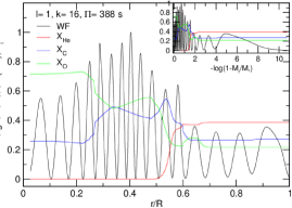
Figure 12: Normalized weight function of the $k=16$ mode (in black) versus the normalized stellar radius. The chemical composition profiles are also indicated by lines with different colors. Inset: the same quantities as in the main figure, but as a function of the negative logarithm of the outer mass fraction.

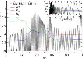
Figure 13: Same as fig. 12, but for the $k=56$ mode.

8 The rotational period

At first glance, the rotation period of PG1159-035 appears well established. Analysis of the K2 modes find an average splitting of $\delta\nu\ =4.0\pm 0.4\ \mu$Hz for $\ell=1$, and $\delta\nu\ =6.8\pm 0.2\ \mu$Hz for $\ell=2$. Using the equations for uniform rotation in the asymptotic limit, we find a rotation frequency of $8.16\ \mu$Hz and a period of $P_{\rm rot}=1.4\pm 0.1$ days. This is in agreement with the $1.38\pm 0.013$ day rotation period reported in Winget et al. (1991) and $1.3935\pm 0.0008$ day period reported in Costa et al. (2008).

The Fourier Tranform of K2 light curve reveals a significant ($1.46$ mma) peak at $8.906\pm 0.003\ \mu\mathrm{Hz}$ as well as its harmonic at $17.811\pm 0.006\,\mu$Hz. The modulation is apparent in visual inspection of the K2 light curve. There is no evidence that PG 1159-035 is a member of a binary system, so we propose that this modulation represents a surface rotation of $1.299\pm 0.001$ days. PG 1159-035 now joins PG 0112+104 (Hermes et al., 2017a) as one of only two WDs with photometrically detected surface rotation frequencies.

If 8.906 $\mu$Hz is the surface rotation frequency and PG 1159-035 rotates as a solid body as proposed by Charpinet et al. (2009), we would expect $\ell$ = 1 triplets with splittings of $\delta\nu\,=4.4\,\mu$Hz and $\ell=2$ quintuplets with $\delta\nu\,=7.4\,\mu$Hz. This predicted $\ell=1$ splitting is at the outer range of permitted values from K2 data. The predicted $\ell=2$ splittings are several sigmas from the values observed.

Figure 14: The observed multiplet splittings for 23 $\ell$ = 1 and 9 $\ell$ = 2 modes (we do not plot the singlets) centered on the $m=0$ component. The $k$ number for each mode is indicated on the right. The dashed and dotted lines indicate the frequency splittings if the star rotates as a rigid body with frequency $\Omega_{\rm rot}=8.16~{}\mu\mathrm{Hz}$. The width and color of the boxes correspond respectively to the uncertainty and the amplitude of the frequencies: the darker the color, the higher the amplitude.

Figure 14 shows the observational frequency splitting of $\ell$ = 1 and $\ell$ = 2 compared with the theoretical splitting, if PG 1159-035 rotates as a rigid body with frequency $\Omega_{\mathrm{rot}}=8.16\ \mu\mathrm{Hz}$. We do not find good agreement.

Figure 15: How far each $\delta\nu_{1}$ is from the median value $\overline{\delta\nu_{1}}$. It was calculated separately for frequency spacings between $m=-1$ and $m=0$ modes (red points) and for frequency spacings between $m=0$ and $m=1$ modes (blue points).

The K2 data shows evidence for two different rotation periods, the first from direct detection of a peak in the FT and a second from the average multiplet structure. If we interpret the rotation period derived from the multiplet structure as a globally averaged rotation rate, this provides evidence that differential rotation plays a role in PG1159-035. Further analysis of differential rotation in PG1159-035 will surely be the subject of future work.

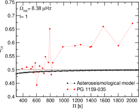
Figure 16: Observed Ledoux rotation coefficients $C(\ell,k)$ (red) versus the predicted ones (black) in the best asteroseismic model, in terms of the periods. The horizontal dotted line corresponding to $C(\ell,k)=0.5$ is the asymptotic value for large radial-order modes. If $\Omega_{\mathrm{rot}}=8.38~{}\mu$Hz, all values are larger than the model ones.

Figure 16 shows the observed Ledoux rotation coefficients $C(\ell,k)$ versus the predicted ones in the best asteroseismic model, which are close to the asymptotic values, for $\Omega_{\mathrm{rot}}=8.38~{}\mu$Hz (Winget et al., 1991). The observed values are in general larger than the predicted ones, indicating second order terms are necessary. If we assume the rotation frequency of $\Omega_{\mathrm{rot}}=8.90~{}\mu$Hz , all values are larger than the model and asymptotic value.

We observed a significant peak (4.29 mma) in the FT of the TESS light curve at 8.66 $\mu$Hz and we used the open source Python package TESS Localize (Higgins & Bell, 2022a) to make sure that this variability comes from PG1159-035. If this frequency is due the surface rotation, then it can indicate that the rotation frequency of the star not only changes radially, but also temporally.

9 Period changes

The evolution of a typical WD is dominated by cooling. An observable effect of WD evolution is change in pulsation periods. Measurements of period change can be used to constrain fundamental physical properties and constrain evolutionary models.

For a typical WD model, we expect the rate of change of period with time $\dot{\Pi}$ values between $10^{-12}-10^{-15}\,\mathrm{s\,s}^{-1}$. Hot WDs evolve rapidly, so higher values of $\dot{\Pi}$ will be associated with hotter stars. PG 1159-035 is very hot ($T_{\mathrm{eff}}\approx 140,000K$) and is evolving quickly. The period changes can be measured directly (e.g. Costa & Kepler, 2008). As PG 1159-035 has not yet completed the contraction of its outer layers, we must also consider the effects of contraction of the stellar atmosphere, which can produce decreasing periods ($\bf\dot{\Pi}<0$).

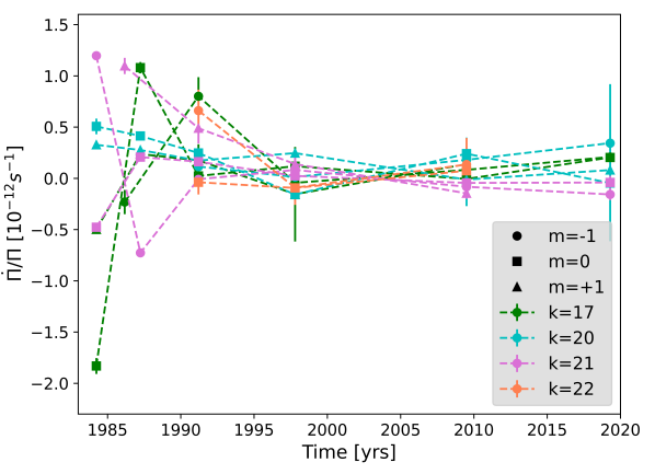
Figure 17: Relative change of pulsation period with time $\frac{\dot{\Pi}}{\Pi}$ over time to $k=17$, $k=20$, $k=21$ and $k=22$ modes. The error bars were calculated by Markov Chain Monte Carlo Simulation.

We used the periods measured in the earlier data cited in Table 1 to calculate the period changes of PG 1159-035’s high-amplitude modes. We choose four modes which often appear in the data. They are the $k=17,20,21,22$ modes, all $\ell=1$. For each given index radial $k$ mode, the period change between two consecutive data sets $n$ and $n+1$ was evaluated as:

$$\frac{\dot{\Pi}}{\Pi}\left(k,t=\frac{t_{n+1}+t_{n}}{2}\right)=\frac{1}{\Pi_{k}(t_{0})}\frac{\Pi_{k}(t_{n+1})-\Pi_{k}(t_{n})}{t_{n+1}-t_{n}}$$ (7)

where $\Pi_{k}(t_{n})$ is the period of index radial $k$ mode observed in the year $t_{n}$ and $t_{0}$ is the year of the first observation for the considered datasets.

The period changes of these modes over the years do not present a clear pattern. However, Figure 17 shows that, overlapping, they look to be converging to some value and then scattering again. The m components of the $\it k$=17 and the $\it k$=21 modes switch between positive and negative $\dot{\Pi}$ values. Clearly, we are neglecting an important effect that acts on timescales of months and years, as nonlinear mode coupling. Other possible effects include reflex motion and proper motion, but these would be expected to act equally on all modes. Magnetic fields would also affect $\dot{\Pi}$, and could affect each mode differently.

10 Combination frequencies

It was previously reported that PG 1159-035 had no combination frequencies, since none were detected in the previous data (e.g. Costa et al., 2008). However, due to the extended time base and signal-to-noise of the K2 data set, for the first time we are able to identify combination frequencies in its pulsation spectrum (see Table 5).

The amplitudes of these frequencies are small, but then so are those of the parent linear modes. A measure of the strength of the nonlinearity is

$$R_{\rm c}\equiv\frac{A_{i+j}}{n_{ij}A_{i}A_{j}}$$ (8)

where $A_{i}$ and $A_{j}$ are the parent amplitudes (in units of modulation amplitude ma), $A_{i+j}$ is the amplitude of the combination frequency, and $n_{ij}=2$ for $i\neq j$ and 1 otherwise (van Kerkwijk et al., 2000; Yeates et al., 2005).

From Table 5 we find $R_{\rm c}$ values in the range $\approx 4$–14. We note that these values are not smaller than those found in the DAVs, and are in fact completely consistent with them (see Yeates et al., 2005).

In the DAVs and DBVs, the dominant mechanism producing combination frequencies and nonlinear light curves is thought to be the interaction of the pulsations with the surface convection zone (Brickhill, 1992a, b; Wu, 2001; Montgomery, 2005). PG 1159-035 is sufficiently hot that models show no surface convection zone (e.g., Werner et al., 1989), so the presence of combination frequencies is something of a mystery, though Kurtz et al. (2015) find multiple large apparent amplitude combination peaks in Slowly Pulsating B stars and $\gamma$ Dor stars, and explain that visibility, which is highly dependent on the surface patterns of oscillations, can explain these amplitudes apparently larger than their parent frequencies.

An alternative mechanism is the nonlinear temperature to flux relationship described in Brassard et al. (1995). While this mechanism is not generally successful in explaining the nonlinearities seen in the DAVs (e.g., Vuille & Brassard, 2000), we consider whether it could be viable for the amplitudes of the combination frequencies observed in the DOV PG 1159-035.

To simplify the calculation, we approximate the stellar flux as a blackbody, $B_{\lambda}(T)$, and expand it to second order in the temperature perturbations, $\Delta T$:

$$F_{\lambda}\approx B_{\lambda}(T_{0})+\frac{\partial B_{\lambda}(T_{0})}{\partial T}\Delta T+\frac{1}{2}\frac{\partial^{2}B_{\lambda}(T_{0})}{\partial T^{2}}(\Delta T)^{2}+\ldots$$ (9)

Assuming just one mode with temperature perturbation $\Delta T_{i}$, we find that the fractional flux perturbations are

$$A_{i} = \frac{1}{B_{\lambda}(T_{0})}\frac{\partial B_{\lambda}(T_{0})}{\partial T}\Delta T_{i}$$ (10)

$$A_{2i} = \frac{1}{2B_{\lambda}(T_{0})}\frac{\partial^{2}B_{\lambda}(T_{0})}{\partial T^{2}}\Delta T_{i}^{2}$$ (11)

with the result that

$$R_{\rm c}=\frac{A_{2i}}{A_{i}^{2}}=\frac{1}{2}B_{\lambda}(T_{0})\left(\frac{\partial B_{\lambda}(T_{0})}{\partial T}\right)^{-2}\frac{\partial^{2}B_{\lambda}(T_{0})}{\partial T^{2}}$$ (12)

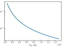
Figure 18: Expected value of $R_{\rm c}$ (Equation 12) as a function of $T_{\rm eff}$ for observations centered on $\lambda=5500\,$Å. A blackbody spectrum was assumed for this calculation.

Frequency ($\mu$Hz)	Amplitude (mma)	Combination frequencies $f_{k}$	Difference ($\mu$Hz)	$R_{\rm c}$
$75.31\pm 0.03$	$0.17\pm 0.05$	$f_{20}-f_{21}$	$-$0.06 (2.1$\,\sigma$)	3.9
$142.74\pm 0.03$	$0.19\pm 0.05$	$f_{20}-f_{22}$	+0.01 (0.5$\,\sigma$)	11.6
$419.28\pm 0.06$	$0.08\pm 0.05$	$f_{17}-f_{22}$	+0.25 (4.2$\,\sigma$)	14.0
$3412.82\pm 0.03$	$0.20\pm 0.05$	$f_{21}+f_{26}$	+0.01 (0.1$\,\sigma$)	9.6
$3716.39\pm 0.02$	$0.24\pm 0.05$	$2f_{21}$	$-$0.01 (0.5$\,\sigma$)	14.4
$3791.56\pm 0.03$	$0.18\pm 0.05$	$f_{20}+f_{21}$	+0.06 (1.7$\,\sigma$)	4.1
$3866.84\pm 0.03$	$0.19\pm 0.05$	$2f_{20}$	+0.03 (0.7$\,\sigma$)	6.7
$4143.67\pm 0.03$	$0.15\pm 0.05$	$f_{17}+f_{20}$	$-$0.03 (1.0$\,\sigma$)	7.5

Table 5: Combination frequencies in K2 data.

In Figure 18, we plot $R_{\rm c}$ as a function of $T$ for observations centered at the wavelength $\lambda=5500\,$Å. At $T_{\rm eff}\approx\,$140,000 K, we see that $R_{\rm c}<0.01$, which is much smaller than the observed values. Thus, if a blackbody spectrum is a good proxy for the actual flux distribution, then the mechanism of Brassard et al. (1995) cannot explain the observed nonlinearities in PG1159-035. However, it is possible that using actual model atmospheres could produce larger values of $R_{\rm c}$, but the atmospheres would need to be calculated on a fine enough grid in $T_{\rm eff}$ that accurate first- and second-order derivatives can be computed. Clearly, understanding the origin of these combination frequencies will require further analysis.

11 Asteroseismic modeling

The location of PG 1159-035 in the $\log T_{\rm eff}-\log g$ plane is displayed in Fig. 19 with a blue dot with error bars. If the star has $T_{\rm eff}=140\,000\pm 5\,000$ K and $\log g=7.0\pm 0.5$ (Werner et al., 2011), the PG 1159 evolutionary tracks of Althaus et al. (2005) and Miller Bertolami & Althaus (2006) indicate that the star has just turned its “evolutionary knee” (maximum $T_{\rm eff}$), and is entering its WD cooling track. The spectroscopic stellar mass of the star, considering the uncertainties in $T_{\rm eff}$ and $\log g$, is derived by linear interpolation and results in $M_{\star}=0.54\pm 0.07M_{\odot}$. We note that the star falls in the region where our pulsation models predict a mix of positive and negative rates of period changes (Fig. 19), as found by Costa & Kepler (2008) (see also Sect. 8).

In the next sections, we first describe the PG 1159 evolutionary models used in this work, and then we apply the tools of WD asteroseismology for inferring the stellar mass and the derivation of an asteroseismic model for PG 1159$-$035. Sect. 6.2 shows that TESS has detected very few periods (see Table 4), and they are almost identical to the corresponding K2 periods. Therefore, we will carry out our asteroseismic modeling considering only the K2 periods (Tables 2 and 3).

Figure 19: Location of the known GW Vir variable stars in the $\log T_{\rm eff}-\log g$ diagram, depicted with small red circles. Thin solid curves show the post-born-again evolutionary tracks from Althaus et al. (2005) and Miller Bertolami & Althaus (2006) for different stellar masses in the range $0.530-0.741M_{\odot}$. The location of the GW Vir stars observed with TESS (with published results) are emphasized with large orange circles. PG 1159$-$035 is displayed with a small blue circle with the error bars (within a box with dotted lines), according to Werner et al. (2011) ($T_{\rm eff}=140\,000\pm 5\,000$ K and $\log g=7\pm 0.5$). The location of PG 1159$-$035 according to the asteroseismic model (see Sect. 11.3) is depicted with a black, small circle. The violet curves divide the plane in three regions: one in which all the $g$ modes have $\dot{\Pi}<0$, another region where some modes have $\dot{\Pi}<0$ and others have $\dot{\Pi}>0$, and finally a region in which all the modes have $\dot{\Pi}>0$. The gray curves correspond to the theoretical blue edge of the GW Vir instability strip for $\ell=1$ and $\ell=2$ $g$ modes, according to Córsico et al. (2006).

11.1 PG 1159 stellar models

The PG1159 star model set used in this work has been described in depth in Althaus et al. (2005) and Miller Bertolami & Althaus (2006, 2007). We refer the interested reader to those papers for details. Althaus et al. (2005) and Miller Bertolami & Althaus (2006) computed the complete evolution of non-rotating model star sequences with initial masses on the ZAMS in the range $1-3.75\ M_{\sun}$ and assuming a metallicity of $Z=0.02$. All the post-AGB evolutionary sequences computed with the LPCODE evolutionary code (Althaus et al., 2005) were followed through the very late thermal pulse (VLTP) and the resulting born-again episode that give rise to the H-deficient, He-, C- and O-rich composition characteristic of PG 1159 stars. The masses of the resulting remnants are $0.530$, $0.542$, $0.565$, $0.589$, $0.609$, $0.664$, and $0.741\ M_{\sun}$. In Fig. 19 the evolutionary tracks employed in this work are shown in the $\log T_{\rm eff}$ vs. $\log g$ plane.

11.2 Derivation of the stellar mass from the period spacings

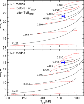
Figure 20: Upper panel: dipole ($\ell=1$) average of the computed period spacings, $\overline{\Delta\Pi_{k}}$, assessed in a range of periods that includes the periods observed in PG 1159$-$035, shown as dashed red (solid black) curves corresponding to stages before (after) the maximum $T_{\rm eff}$ for different stellar masses. The location of PG 1159$-$035 when we use the effective temperature derived by Werner et al. (2011), $T_{\rm eff}=140\,000\pm 5\,000$ K, and the period spacing $\Delta\Pi_{1}=21.28\pm 0.02$ s derived in Sect. 6, is highlighted with a blue circle. Lower panel: same as in upper panel, but for the case in which the period spacing is assumed to be associated to $\ell=2$ modes ($\Delta\Pi_{2}=13.02\pm 0.04$ s).

The approach we use to extract information on the stellar mass of PG 1159$-$035 is the same employed in, e.g., Córsico et al. (2021). Briefly, a way to estimate the masses of GW Vir stars is by comparing the observed period spacing $\Delta\Pi$ with the asymptotic period spacing $\Delta\Pi_{\ell}^{\rm a}$ (Tassoul et al., 1990) at the effective temperature of the star, following the pioneering work of Kawaler (1988). Since GW Vir stars generally do not have all of their pulsation modes in the asymptotic regime, and are not chemically homogeneous, it is more reliable to infer the stellar mass by comparing $\Delta\Pi$ with the average of the computed period spacings ($\overline{\Delta\Pi_{k}}$). It is assessed as $\overline{\Delta\Pi_{k}}=(n_{\rm c}-1)^{-1}\sum_{k=1}^{n_{\rm c}}\Delta\Pi_{k}$, where the “forward” period spacing ($\Delta\Pi_{k}$) is defined as $\Delta\Pi_{k}=\Pi_{k+1}-\Pi_{k}$ ($k$ being the radial order) and $n_{\rm c}$ is the number of computed periods laying in the range of the observed periods. Note that this method for assessing the stellar mass relies on the spectroscopic effective temperature, and the results are unavoidably affected by its associated uncertainty.

We have calculated the average of the computed period spacings for $\ell=1$ and $\ell=2$, in terms of the effective temperature, for all the masses considered. We employed the LP-PUL pulsation code (Córsico & Althaus, 2006) for computing the dipole and quadrupole adiabatic periods of $g$ modes on fully evolutionary PG1159 models generated with the LPCODE evolutionary code (Althaus et al., 2005). The results are shown in the upper ($\ell=1$) and lower ($\ell=2$) panels of Fig. 20, where we show $\overline{\Delta\Pi_{k}}$ corresponding to evolutionary stages before the maximum possible effective temperature, ${T_{\rm eff}}^{\rm MAX}$, which depends on the stellar mass, with red dashed lines, and the phases after that ${T_{\rm eff}}^{\rm MAX}$, the so-called WD stage itself, with solid black lines. The location of PG 1159$-$035 is indicated by a small blue circle with error bars, and corresponds to the effective temperature of the star according to Werner et al. (2011) and the period spacings derived in Sect. 6. We perform linear interpolations between the sequences and obtain the stellar mass shown in Table 6. If the star is after the “evolutionary knee”, as suggested by its spectroscopic parameters (see Fig. 19), then the stellar mass is $\sim 0.58M_{\odot}$ according to the $\ell=1$ modes, and $\sim 0.54M_{\odot}$ according to the $\ell=2$ modes.

	$\ell=1$	$\ell=2$
Before the maximum $T_{\rm eff}$	$0.594^{+0.003}_{-0.002}$	$0.560^{+0.005}_{-0.018}$
After the maximum $T_{\rm eff}$	$0.576^{+0.005}_{-0.004}$	$0.538^{+0.004}_{-0.002}$

Table 6: Stellar mass (in $M_{\odot}$) derived for PG 1159$-$035 by comparing the the average of the computed period spacings ($\overline{\Delta\Pi_{k}}$) of our PG 1159 models with the observed period spacings derived in Sect. 6.

If the star were at an earlier stage, before the“evolutionary knee”, the mass would be $\sim 0.59M_{\odot}$ and $\sim 0.54M_{\odot}$, according to the modes with $\ell=1$ and $\ell=2$, respectively. We conclude that the stellar mass of PG 1159$-$035, as derived from its period spacings $\Delta\Pi_{1}$ and $\Delta\Pi_{2}$, is in the range $0.54-0.59M_{\odot}$. This range of masses is compatible with the spectroscopic mass, $M_{\star}=0.54\pm 0.07\,M_{\odot}$ (Werner et al., 2011).

11.3 Asteroseismic period fits

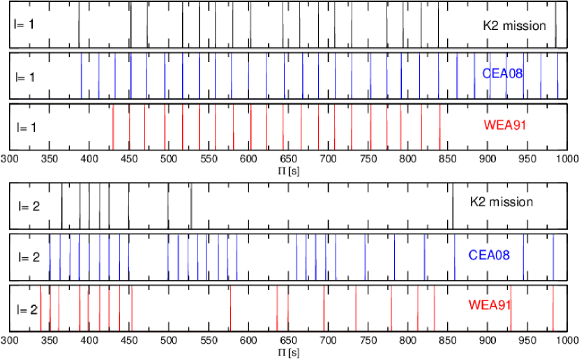
Figure 21: Schematic distribution of the $\ell=1$ and $\ell=2$ ($m=0$) pulsation periods of PG 1159$-$035 observed by K2 (black lines, upper panels), observed by Costa et al. (2008) (CEA08, blue lines, middle panels), and observed by Winget et al. (1991) (WEA91, red lines, lower panels). At least 14 additional $\ell=1$ modes only detected by K2 at periods longer than 1000 s have been cut off and not shown here, but are detailed in Table 2. The amplitudes have been arbitrarily set to one for clarity.

An asteroseismic tool to disentangle the internal structure of GW Vir stars is to search for theoretical models that best match the individual pulsation periods of the target star. To measure the goodness of the agreement between the theoretical periods ($\Pi_{\ell,k}$) and the observed periods ($\Pi_{i}^{\rm o}$), we adopt the quality function: $\chi^{2}(M_{\star},T_{\rm eff})=\frac{1}{N}\sum_{i=1}^{N}{\rm min}[(\Pi_{\ell,k}-\Pi_{i}^{\rm o})^{2}]$ (Córsico et al., 2021), where $N$ is the number of observed periods. In order to find the stellar model that best replicates the observed periods exhibited by each target star – the “asteroseismic” model –, we assess the function $\chi^{2}$ for stellar model masses $M_{\star}=0.530,0.542,0.565,0.589,0.609,0.664$, and $0.741M_{\odot}$. For the effective temperature, we employ a much finer grid ($\Delta T_{\rm eff}=10-30$ K). The PG 1159 model that shows the lowest value of $\chi^{2}$ is adopted as the best-fit asteroseismic model.

$\Pi_{i}^{\rm O}$	$\ell^{\rm O}$	$\Pi_{k}$	$\ell$	$k$	$\delta\Pi_{k}$	$\dot{\Pi}_{k}$	Unstable
(s)		(s)			(s)	($10^{-11}$ s/s)
(387.19)	1	388.29	1	16	$-1.10$	1.11	no
452.45	1	452.46	1	19	$-0.01$	1.15	no
473.06	1	474.24	1	20	$-1.18$	0.81	no
517.22	1	515.69	1	22	1.53	1.22	no
538.16	1	537.78	1	23	0.38	1.07	no
558.45	1	557.60	1	24	0.85	0.60	no
580.40	1	579.02	1	25	1.38	1.29	no
(602.35)	1	601.90	1	26	0.45	1.22	no
643.24	1	642.93	1	28	0.31	1.51	no
664.20	1	665.31	1	29	$-1.11$	1.07	no
687.74	1	685.85	1	30	1.89	1.01	no
708.12	1	707.25	1	31	0.87	1.60	no
729.58	1	728.55	1	32	1.03	1.30	no
773.71	1	771.82	1	34	1.89	1.49	no
793.95	1	793.26	1	35	0.69	1.85	no
816.74	1	814.77	1	36	1.97	1.31	no
838.36	1	836.14	1	37	2.22	1.66	no
985.65	1	987.59	1	44	$-1.94$	1.87	no
1116.01	1	1120.53	1	50	$-4.52$	2.62	no
1164.88	1	1163.72	1	52	1.16	2.95	no
1246.27	1	1251.47	1	56	$-5.20$	1.95	no
1284.52	1	1273.97	1	57	10.55	3.32	no
1387.06	1	1383.81	1	62	3.25	3.62	no
1406.51	1	1405.39	1	63	1.12	2.37	no
1539.03	1	1538.67	1	69	0.36	3.45	no
1555.74	1	1560.10	1	70	$-4.36$	3.27	no
1580.08	1	1581.27	1	71	$-1.19$	3.58	no
1802.11	1	1802.75	1	81	$-0.64$	4.03	no
1982.78	1	1981.36	1	89	1.42	5.18	no
2010.07	1	2002.26	1	90	7.81	3.15	no
2084.71	1	2091.45	1	94	$-6.74$	6.57	no
2807.93	1	2804.11	1	126	3.82	9.17	no
365.54	2	364.02	2	27	1.52	0.70	no
(388.18)	2	388.36	2	29	$-0.18$	0.51	no
400.08	2	400.67	2	30	$-0.59$	0.88	no
(413.22)	2	413.73	2	31	$-0.51$	0.93	no
(425.00)	2	425.42	2	32	$-0.42$	0.72	no
449.36	2	450.18	2	34	$-0.82$	1.18	no
498.74	2	500.55	2	38	$-1.81$	1.28	no
528.21	2	524.37	2	40	3.84	1.10	no
856.56	2	852.23	2	66	4.33	1.62	no

Table 7: Observed $m=0$ and theoretical periods of the asteroseismic model for PG 1159$-$035 [$M_{\star}=0.565M_{\odot}$, $T_{\rm eff}=129\,600$ K, $\log(L_{\star}/L_{\odot})=2.189$]. Periods are in seconds and rates of period change (theoretical) are in units of $10^{-11}$ s/s. $\delta\Pi_{i}=\Pi^{\rm O}_{i}-\Pi_{k}$ represents the period differences, the model $\ell$ the harmonic degree, $k$ the radial order, $m$ the azimuthal index. The last column provides information about the pulsational stability/instability nature of the modes. Parenthesis indicate $m=0$ periods which are actually absent from the power spectrum, their values being estimated by averaging the components $m=\pm 1$.

We employ the periods identified with $\ell=1$ and $\ell=2$ modes of Tables 2 and 3, respectively. We consider only $m=0$ components in the case of multiplets. When frequency multiplets have the central component ($m=0$) absent, we adopt a value for this frequency, estimating it as the mean value between the components $m=-1$ and $m=+1$ (if both frequencies exist). We have 32 $\ell=1$ periods and 9 $\ell=2$ periods available to perform the period fits. These periods are shown in Table 7, and they are also plotted in Fig. 21, along with the $m=0$ periods of Winget et al. (1991) (WEA91) and Costa et al. (2008) (CEA08). Regarding $\ell=1$ modes (the 3 upper panels in Fig. 21), we can observe that, in general, the periods which are common to the three data sets are in excellent agreement with each other. This is encouraging, because the results of the previous works, obtained from extensive ground-based observations, are confirmed with the new space data. Second, we can notice that for periods shorter than $\sim 1000$ s, the K2 observations have fewer periods than those of WEA91 and CEA08. Finally, we draw attention to the fact that in the K2 data there are many periods longer than $\sim 1000$ s, which are not present in the sets derived from ground-based observations. These are new periods of PG 1159$-$035. These long periods were not detectable by ground-based observations, mainly because of the relatively short length of each data set and the variable effects of extinction due to the Earth’s atmosphere. These effects generate frequency dependent noise, limiting sensitivity to longer periods. As for $\ell=2$ modes (the 3 lower panels in Fig. 21), we note again much fewer periods in the K2 observations compared to the other two data sets. On the other hand, there is good agreement between the K2 periods and those of CEA08. We also note, in passing, that the periods from WEA91 longer than $\sim 500$ s are somewhat different from those of CEA08, possibly due to alias contamination in the older data sets.

Quantity	Spectroscopy	Asteroseismology
	Astrometry	(This work)
$T_{\rm eff}$ [K]	$140\,000\pm 5\,000^{\rm(a)}$	$129\,600\pm 2\,000$
$M_{\star}$ [$M_{\odot}$]	$0.54\pm 0.07$	$0.565\pm 0.008$
$\log g$ [cm/s2]	$7.0\pm 0.5^{\rm(a)}$	$7.41\pm 0.11$
$\log(L_{\star}/L_{\odot})$	$2.58\pm 0.29^{\rm(a)}$	$2.19\pm 0.04$
$\log(R_{\star}/R_{\odot})$	$\cdots$	$-1.61\pm 0.05$
$M_{\rm env}$ [$M_{\odot}$]	$\cdots$	$0.017$
$(X_{\rm He},X_{\rm C},X_{\rm O})_{\rm s}$	0.33, 0.48, 0.17(a)	0.386, 0.321, 0.217
$d$ [pc]	$592\pm 21^{\rm(b)}$	$444^{+69}_{-59}$
$\pi$ [mas]	$1.69\pm 0.06^{\rm(b)}$	$2.25^{+0.35}_{-0.30}$
$A_{\rm V}$	$\cdots$	$0.064^{+0.002}_{-0.001}$

Table 8: The main characteristics of the GW Vir star PG 1159$-$035. The second column corresponds to spectroscopic and astrometric results, whereas the third column present results from the asteroseismic model of this work.

References: (a) Werner et al. (2011); (b) Gaia (https://gea.esac.esa.int/archive/).

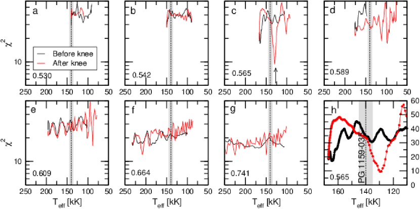
Figure 22: The quality function of the period fit in terms of the effective temperature for the PG 1159 sequences with different stellar masses (in solar units), indicated at the left-bottom corner of each panel. Black (red) lines correspond to stages before (after) the ”evolutionary knee” (see Fig. 19). Only the periods with $m=0$ (see Tables 2 and 3) have been considered. There is a strong minimum in panel c (marked with an arrow), corresponding to a model with $M_{\star}=0.565M_{\odot}$ and $T_{\rm eff}\simeq 129\,600$ K. Panel h is a zoom of the region with the strong minimum seen in panel c; the $y$-axis scale is linear in this case. The vertical dashed line is the spectroscopic $T_{\rm eff}$ of PG 1159$-$035 (140 kK) and the gray zone depicts its 1$\sigma$ uncertainty ($\pm 5$ kK).

The results of our period-to-period fit using the K2 periods are shown in Fig. 22, in which we depict the quality function of the period fit in terms of $T_{\rm eff}$ for the PG 1159 sequences with different stellar masses. Black (red) lines correspond to stages before (after) the“evolutionary knee” (see Fig. 19). There is a very pronounced minimum of the quality function, corresponding to a model of $M_{\star}=0.565M_{\odot}$ and $T_{\rm eff}=129\,613$ K. This model produces the best agreement between observed and theoretical periods. Note that this model is outside the 1$\sigma$ $T_{\rm eff}$ range indicated by the spectroscopy. We have also carried out an additional period fit ignoring the modes with $\ell=2$, and only fitting the modes $\ell=1$. The result of that period fit indicates the same $\chi^{2}$ minimum as in the case of the mode fitting with $\ell=1$ and $\ell=2$. We conclude that this model constitutes the asteroseismic model for PG 1159$-$035. This model is very similar to the one derived by Córsico et al. (2008) considering the Winget et al. (1991) and Costa et al. (2008) period sets, only differing slightly in temperature. Indeed, the current model is $\sim 1600$ K hotter than the model derived by Córsico et al. (2008). The adopted asteroseismic model corresponds to an evolutionary stage just after the star reaches its maximum effective temperature (${T_{\rm eff}}^{\rm MAX}=167\,000$ K; see Fig. 19).

In Table 7 we show a detailed comparison of the observed periods of PG 1159$-$035 and the theoretical $m=0$ periods of the asteroseismic model. To quantitatively assess the quality of the period fit, we compute the average of the absolute period differences, $\overline{\delta\Pi_{i}}=\left(\sum_{i=1}^{N}|\delta\Pi_{i}|\right)/N$, where $\delta\Pi_{i}=(\Pi_{\ell,k}-\Pi_{i}^{\rm o})$ and $N=41$, and the root-mean-square residual, $\sigma=\sqrt{(\sum_{i=1}^{N}|\delta\Pi_{i}|^{2})/N}=\sqrt{\chi^{2}}$. We obtain $\overline{\delta\Pi_{i}}=2.12$ s and $\sigma=3.08$ s. To have a global indicator of the goodness of the period fit that considers the number of free parameters, the number of fitted periods, and the proximity between the theoretical and observed periods, we computed the Bayes Information Criterion (BIC; Koen & Laney, 2000): ${\rm BIC}=n_{\rm p}\left(\frac{\log N}{N}\right)+\log\sigma^{2}$, where $n_{\rm p}$ is the number of free parameters of the models, and $N$ is the number of observed periods. The smaller the value of BIC, the better the quality of the fit. In our case, $n_{\rm p}=2$ (stellar mass and effective temperature), $N=41$, and $\sigma=3.08$ s. We obtain ${\rm BIC}=1.06$, which means that our period fit is acceptable. In comparison, Córsico et al. (2021) obtain ${\rm BIC}=0.59$ for the PNNV star RX J2117+3412, ${\rm BIC}=1.18$ for the hybrid DOV star HS 2324+3944, ${\rm BIC}=1.15$ for the PNNV star NGC 1501, and ${\rm BIC}=1.20$ for the PNNV star NGC 2371. On the other hand, Córsico et al. (2022) and Bischoff-Kim et al. (2019) obtain ${\rm BIC}=1.13$ and ${\rm BIC}=1.20$, respectively, for the prototypical star of the DBVs class of pulsating WDs, GD 358. The asteroseismic model for PG 1159$-$035 has $(\overline{\Delta\Pi_{k}})_{\ell=1}=22.02$ s and $(\overline{\Delta\Pi_{k}})_{\ell=2}=12.60$ s, in agreement with the measured values, $\Delta\Pi_{1}=21.28$ s and $\Delta\Pi_{2}=13.02$ s.

We also include in Table 7 (column 7) the rates of period change ($\dot{\Pi}\equiv d\Pi/dt$) predicted for each $g$ mode of PG 1159$-$035 according to the asteroseismic model. Note that all of them are positive ($\dot{\Pi}>0$), implying that the periods in the model are lengthening over time. The rate of change of periods in WDs and pre-WDs is related to the rate of change of temperature with time $\dot{T}$ ($T$ being the temperature at the region of the period formation) and $\dot{R_{\star}}$ ($R_{\star}$ being the stellar radius) through the order-of-magnitude expression $(\dot{\Pi}/\Pi)\approx-a\ (\dot{T}/T)+b\ (\dot{R_{\star}}/R_{\star})$ (Winget et al., 1983), $a,b$ being positive constants close to 1. According to our asteroseismic model, the star is entering its cooling stage after reaching its maximum temperature (Fig. 19). As a consequence, $\dot{T}<0$ and $\dot{R_{\star}}<0$ with $|-a\ (\dot{T}/T)|>|b\ (\dot{R_{\star}}/R_{\star})|$, and then, $\dot{\Pi}>0$. Our best fit model has all the modes with $\dot{\Pi}>0$, and thus it does not reproduce the measurements of Costa & Kepler (2008) neither the values shown in Fig. 17 of the present paper, which indicate that the pulsation modes of PG 1159$-$035 have positive and negative values of $\dot{\Pi}$ (see Fig. 19). Also, the magnitude of the observed rates of period change in PG 1159$-$035 are larger than the values derived from the asteroseismic model. This may be because the star could have a very thin He envelope, which would inhibit nuclear burning and shorten the evolutionary timescale (Althaus et al., 2008). This would result in larger rates of period change. We also note that our models do not include radiative levitation, which might influence the change in position of the nodes of the eigenfunctions of the pulsation modes, and the photospheric abundances in hot WDs depend on the balance between the flow of matter sinking under gravity and the resistance due to radiative levitation, as well as on the weak residual wind, driven by the metal opacities. It is also possible that the observed period changes are not attributable to stellar evolution, but to another (unknown) mechanism. For instance, in the case of the DOV star PG 0122+200, the detected rates of period changes are much larger than the theoretical models predict as due simply to evolutionary cooling, and it is suggested that the resonant coupling induced within rotational triplets could be the mechanism operating there (Vauclair et al., 2011).

In Table 8, we list the main characteristics of the asteroseismic model for PG 1159$-$035. The quoted uncertainties in the stellar mass and the effective temperature of the best fit model ($\sigma_{\rm M_{*}}$ and $\sigma_{T_{\rm eff}}$) are internal errors resulting from the period fit procedure alone, and are assessed according to the following expression, derived by Zhang et al. (1986):

$$\sigma_{i}^{2}=\frac{d_{i}^{2}}{S-S_{0}}$$ (13)

where $S_{0}=\chi^{2}(M_{*}^{0},T_{\rm eff}^{0})$ is the absolute minimum of $\chi^{2}$ which is reached at ($M_{*}^{0},T_{\rm eff}^{0}$) corresponding to the best-fit model, and $S$ the value of $\chi^{2}$ when we change the parameter $i$ (in our case, $M_{*}$ or $T_{\rm eff}$) by an amount $d_{i}$ keeping fixed the other parameter. The quantity $d_{i}$ can be evaluated as the minimum step in the grid of the parameter $i$. We have $d_{T_{\rm eff}}\equiv\Delta T_{\rm eff}\sim 1000$ K and $d_{M_{*}}\equiv\Delta M_{*}$ in the range $0.009-0.024M_{\odot}$. The rest of the uncertainties are calculated based on those in mass and effective temperature. The effective temperature of the asteroseismic model is lower than the spectroscopic effective temperature $T_{\rm eff}$ of PG 1159$-$035. The seismic stellar mass ($0.565\pm 0.008M_{\odot}$) is consistent with the range of masses indicated by the period spacings of PG 1159$-$035 ($0.54\lesssim M_{\star}/M_{\odot}\lesssim 0.58$), and compatible with the spectroscopic mass ($M_{\star}=0.54\pm 0.07M_{\odot}$). The luminosity of the asteroseismic model, $\log(L_{\star}/L_{\sun})=2.19\pm 0.04$ is $\sim 20$% lower than the luminosity inferred by Werner et al. (2011), $\log(L_{\star}/L_{\sun})=2.58$, based on the spectroscopic $T_{\rm eff}$ and the evolutionary tracks of Miller Bertolami & Althaus (2006), the same that we use in the present paper.

In Fig. 23 we display the fractional abundances ($X_{i}$) of the main chemical species, ⁴He, ¹²C, ¹³C, and ¹⁶O, corresponding to our best asteroseismic model of PG 1159$-$035, with $M_{\star}=0.565M_{\odot}$ and $T_{\rm eff}=129\,600$ K. The chemical transition regions of O/C and O/C/He are emphasized with gray bands. The precise location, thickness, and steepness of these chemical transition regions fix the mode-trapping properties of the model (see, e.g., Córsico & Althaus, 2005, 2006, for details). Note that the chemical composition in the models are not free parameters, but the result of the evolutionary calculation. It is therefore not an asteroseismic determination of the envelope composition.

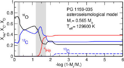
Figure 23: Internal chemical profile of the asteroseismic model of PG 1159$-$035 ($M_{\star}=0.565M_{\sun}$, $T_{\rm eff}=129\,600$ K) in terms of the outer fractional mass. The locations of the O/C and O/C/He chemical interfaces are indicated with gray regions.

11.4 Nonadiabatic analysis

Table 7 also provides information about the pulsational stability/instability nature of the modes associated with the periods fitted to the observed ones (eight column). We examined the sign and magnitude of the computed linear nonadiabatic growth rates $\eta_{k}=-\Im(\sigma_{k})/\Re(\sigma_{k})$, where $\Re(\sigma_{k})$ and $\Im(\sigma_{k})$ are the real and the imaginary parts, respectively, of the complex eigenfrequency $\sigma_{k}$. We have employed the nonadiabatic version of the LP-PUL pulsation code (Córsico et al., 2006), that assumes the “frozen-in convection” approximation (Unno et al., 1989). A positive value of $\eta_{k}$ means that the mode is linearly unstable.

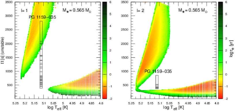
Figure 24: Left panel: periods of excited $\ell=1$ $g$ modes as a function of the effective temperature, with the palette of colors (right scale) indicating the logarithm of the $e$-folding time ($\tau_{\rm e}$ in years), for the PG 1159 sequence with $M_{\star}=0.565M_{\odot}$. Right panel: same as left panel, but for $\ell=2$ modes. In both panels, the pulsation periods with the identification of $\ell$ according to our asteroseismic model (see Table 7), are shown as horizontal segments, where their widths represent the possible $T_{\rm eff}$ interval, according to the best asteroseismic model (Table 8).

We show in Fig. 24 the periods of excited $\ell=1$ (left panel) and $\ell=2$ (right panel) $g$ modes as a function of the effective temperature for the sequence of PG 1159 models with $M_{\star}=0.565M_{\odot}$. In both panels, the identified pulsation periods of PG 1159$-$035 (see Table 7), are shown as horizontal segments, where the segment length represents the $T_{\rm eff}$ range from the best asteroseismic model (Table 8). For the effective temperature and stellar mass of the asteroseismic model, all the $\ell=1$ $g$ modes (left panel) are pulsationally stable, in disagreement with the existence of $\ell=1$ excited modes in PG 1159$-$035. Excited periods predicted by higher $T_{\rm eff}$ models (at the left of the left panel) could explain the long periods shown by the star. However, this instability branch corresponds to models that are before the maximum $T_{\rm eff}$ of the sequence. Our non-adiabatic $g$-mode calculations are not able to reproduce the excited periods in the star. Regarding the $\ell=2$ modes (right panel), our stability computations predict instability for modes with periods in the range $68-316$ s, thus excluding the interval of quadrupole periods excited in PG 1159$-$035 ($365-856$ s). We conclude that our asteroseismic model, while able to closely reproduce the periods observed in PG 1159$-$035, fails to predict their excitation, if the star is after the maximum temperature knee.

We expanded our analysis to include the stability of $\ell=1$ and $\ell=2$ modes for PG 1159 model sequences with $M_{\star}=0.530M_{\odot}$ and $M_{\star}=0.542M_{\odot}$ that embrace PG 1159-035’s spectroscopic mass. The results are displayed in Figs. 25 and 26. The nonadiabatic calculations for these masses predict unstable $\ell=1$ modes with periods up to $\sim 1000$ s, and unstable $\ell=2$ modes with periods up to $\sim 600$ s. However, $\ell=1$ modes with periods longer than $\sim 1000$ s and $\ell=2$ modes with periods longer than $\sim 600$ s are predicted to be pulsationally stable.

In summary, non-adiabatic calculations considering the best asteroseismic model for PG 1159-305, or adopting stellar models within the range of PG 1159-035’s spectroscopic mass are unable to predict the excitation of the long-period $\ell=1$ and $\ell=2$ modes detected in this star with the data of the K2 mission. It is interesting to note that, for GW Vir stars that are evolving at an stage after the ”evolutionary knee”, current non-adiabatic calculations do not predict the excitation of $g$ modes with periods longer than $\sim 1000$ s (Saio, 1996; Gautschy, 1997; Gautschy et al., 2005; Córsico et al., 2006; Quirion et al., 2007). We note, in passing, that these results are robust since in the case of these very hot stars, the pulsational stability analyzes are not affected by typical uncertainties related to convection/pulsation interaction, since PG 1159 stars probably do not have significant outer convective zones. In summary, the existence of very long periods in this DOV star is uncertain. A possible explanation is that these modes are the result of nonlinear combination (difference) frequencies (see Sect. 10).

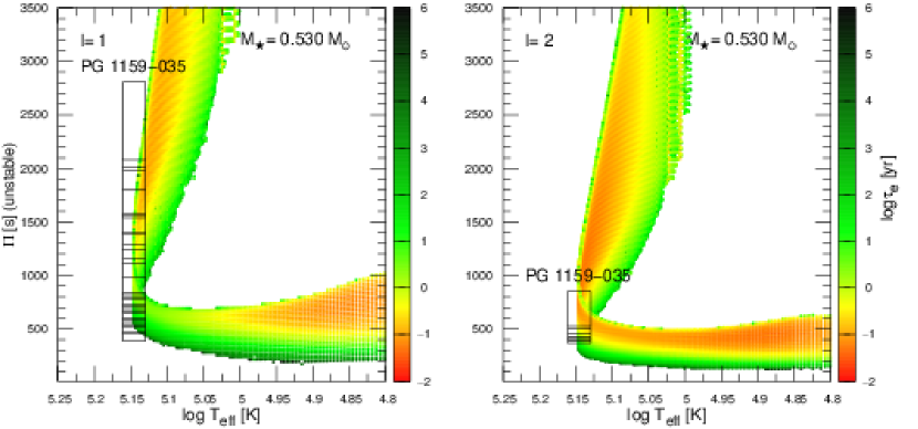
Figure 25: Left panel: periods of excited $\ell=1$ $g$ modes as a function of the effective temperature, with the palette of colors (right scale) indicating the logarithm of the $e$-folding time ($\tau_{\rm e}$ in years), for the PG 1159 sequence with $M_{\star}=0.530M_{\odot}$. In this case, the effective temperature and its uncertainties (horizontal segments) correspond to the spectroscopic determination of Werner et al. (2011). Right panel: same as left panel, but for $\ell=2$ modes. In both panels, the pulsation periods with the identification of $\ell$ according to our asteroseismic model (see Table 7), are shown as horizontal segments, where their widths represent the possible $T_{\rm eff}$ interval, according to spectroscopy (Table 8).

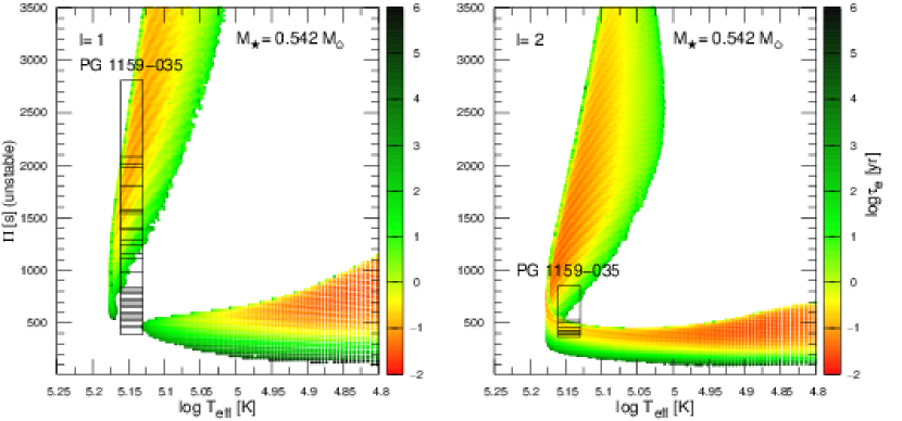
Figure 26: Left panel: periods of excited $\ell=1$ $g$ modes as a function of the effective temperature, with the palette of colors (right scale) indicating the logarithm of the $e$-folding time ($\tau_{\rm e}$ in years), for the PG 1159 sequence with $M_{\star}=0.542M_{\odot}$. Right panel: same as left panel, but for $\ell=2$ modes. In both panels, the pulsation periods with the identification of $\ell$ according to our asteroseismic model (see Table 7), are shown as horizontal segments, where their widths represent the possible $T_{\rm eff}$ interval, according to spectroscopy (Table 8).

We close this section by noting that the precise location of the boundaries of the GW Vir instability domain depends sensitively on the precise value of the abundances of C and O in the driving region of the stars (Quirion et al., 2004). In particular, by varying moderately the C and O abundances at the driving region, the blue edges of the GW Vir instability strip can be substantially shifted to higher or lower effective temperatures, according to the extensive calculations of Quirion et al. (2007). For instance, if the O abundance changes from 20% to 40%, with the C abundance fixed at 40%, the blue edge of the instability strip for $\ell=1$ $g$ modes gets hotter by $\sim 10\,000$ K (see Fig. 32 of Quirion et al., 2007). We conclude that a reasonable contrast in the O and C abundances at the driving region of PG 1159$-$035 in relation to the atmospheric abundances, could alleviate the discrepancy between the location of our asteroseismic model and the very existence of pulsations in this star.

11.5 Asteroseismic distance

The asteroseismic distance to PG 1159$-$035 can be computed as in Uzundag et al. (2021). Based on the luminosity of the asteroseismic model, $\log(L_{\star}/L_{\odot})=2.19\pm 0.04$, and a bolometric correction $BC=-7.6\pm 0.2$ from Kawaler & Bradley (1994) (estimated from Werner et al., 1991), the absolute magnitude can be assessed as $M_{\rm V}=M_{\rm B}-BC$, where $M_{\rm B}=M_{{\rm B},\odot}-2.5\ \log(L_{\star}/L_{\odot})$. We employ the solar bolometric magnitude $M_{\rm B\odot}=4.74$ (Cox, 2000). The seismic distance $d$ is derived from the relation: $\log d=[m_{\rm V}-M_{\rm V}+5-A_{\rm V}(d)]/5$. We employ the interstellar extinction law of Chen et al. (1998) for $A_{\rm V}(d)$, which is a nonlinear function of the distance and also depends on the Galactic latitude ($b$). For the equatorial coordinates of PG 1159$-$035 (Epoch B2000.00, $\alpha=12^{h}01^{m}45.97^{s}$ and $\delta=-03^{d}45^{\prime}40.62^{"}$) the corresponding Galactic latitude is $b=56.8646$. We use the apparent visual magnitude $m_{\rm V}=15.04\pm 0.01$ (Faedi et al., 2011), and obtain the seismic distance and parallax $d=444^{+69}_{-59}$ pc and $\pi=2.25^{+0.35}_{-0.30}$ mas, respectively, using the extinction coefficient $A_{\rm V}=0.064^{+0.002}_{-0.001}$. A significant check for the validation of the asteroseismic model for PG 1159$-$035 is the comparison of the seismic distance with the distance derived from astrometry. We have available the estimates from Gaia, $d_{\rm G}=592\pm 21$ pc and $\pi_{\rm G}=1.691\pm 0.06$ mas. They are in agreement at $1.5\sigma$ level with the asteroseismic derivations, considering the uncertainties in both determinations, in particular the large asteroseismic luminosity uncertainty.

12 Conclusions

The amount of asteroseismological information available in a pulsating star is directly proportional to the number of detected independent pulsation modes. PG 1159-035 is a complex pulsator and rich target for asteroseismic investigation. We first summarize PG 1159-035’s pulsational properties, as revealed in the K2 and TESS light curves. Our analysis produced a total of 107 frequencies distributed in 44 separate modes and 9 combination frequencies. The modes include 32 $\ell=1$ modes and 12 $\ell=2$ modes. Our investigation of the detected frequencies reveals:

• 15 $\ell=1$ modes consistent with a symmetric $m$ splitting of $\delta\nu=4.0\pm 0.4\ \mu$Hz.

• 9 $\ell=1$ modes with asymmetric $m$ splitting. These modes show $\delta\nu=4.08\pm 0.01\ \mu$Hz between $m=0$ and 1 and $\delta\nu=2.83\pm 0.06\ \mu$Hz between $m=0$ and $-1$. The asymmetries are not explained by the presence of a simple magnetic field geometry. We must caution that the asymmetric modes can also be explained by combination frequencies, following Kurtz et al. (2015).

• 9 $\ell=1$ modes with single peaks lacking multiplet structure.

• 12 $\ell=2$ modes with an average splitting of $\delta\nu=6.8\pm 0.2\ \mu$Hz. We note that none of the $\ell=2$ modes are complete quintuplets.

• the identification of a possible surface rotational frequency at $8.904\pm 0.003\ \mu$Hz, as well as its harmonic at $17.813\pm 0.006\ \mu$Hz, which is roughly 9 per cent faster than the rotation frequency inferred from the $\ell=1,2$ multiplet splittings.

• 9 combination frequencies.

• Several modes with periods between 400 and 1000 seconds show Lorentzian widths consistent with coherence timescale shorter than the observation length.

• The rates of period change for the highest amplitude modes, separately, do not show a clear pattern and can switch between positive and negative values. But, overlapping, they look to be converging to some value and then scattering again.

• the $\ell=1$ modes form a sequence with an average period spacing of $21.28\pm 0.02$ s.

• the $\ell=2$ modes form a sequence with an average period spacing of $12.97\pm 0.4$ s.

PG 1159-035 joins the hot DBV PG 0112+104 as the second WD with a photometrically detected surface rotation frequency. The $8.9\ \mu$Hz frequency represents a surface rotation rate of $1.299\pm 0.002$ days. The frequency splittings of the $\ell=1$ and $\ell=2$ modes indicate a rotation period of $1.4\pm 0.1$ days. The individual modes sample the rotation in different regions of the star, and we find that the rotational splittings are not constant with the radial node $k$ value. In particular, the high k $\ell$ = 1 modes that preferentially sample the outer atmosphere show asymmetric splittings. Taken together, PG 1159$-$035’s pulsation structure and the surface rotation period provide evidence of nonuniform rotation. PG 1159-035 is an important object for future analysis of the effects of differential rotation and internal structure in a DOV star.

We also present the first detection of combination frequencies in PG 1159-035. Surface convection is not expected to play a role in this hot object. We find that the fractional temperature changes required to produce the observed pulsation amplitudes are $\approx$ 2.5 times than that of a 12,000 K DAV WD. The second order nonlinearities are correspondingly larger, making the nonlinear response of flux to small temperature changes a plausible mechanism to produce combination frequencies in PG 1159-035. The second part of this work focuses on using the detected frequencies to complete a detailed asteroseismic investigation of PG 1159-035. We summarize the results:

• The average period spacings for $\ell=1$ and $\ell=2$ give a mass range of $0.54-0.59M_{\odot}$ consistent with the spectroscopic mass.

• The detailed asteroseismic fit includes new high k modes not included in previous studies.

• The best adiabatic asteroseismic fit model has $T_{\rm eff}=129,600\pm 2\,000$ K, $M_{\star}=0.565\pm 0.008\ M_{\odot}$, $\log g=7.41\pm 0.11$, $\log(L_{\star}/L_{\odot})=2.19\pm 0.04$, $\log(R_{\star}/R_{\odot})=-1.61\pm 0.05$, and $M_{\rm env}=0.017$ $M_{\odot}$.

• The best fit model corresponds to an evolutionary stage just after the star reaches its maximum effective temperature.

• The luminosity of the best fit model is consistent at $1.5\sigma$ level with the astrometric parallax from Gaia.

• The rates of period change predicted by the best-fit model are positive for all modes, and thus it do not agree with the observed positive and negative values.

• A nonadiabatic analysis considering the best-fit asteroseismic model is unable to predict the excitation of any of the periods detected in PG 1159-035. However, representative models of the star according to its spectroscopic parameters are able to predict the unstable periods, except for the long periods ($\Pi\gtrsim 1000$ s) associated to $\ell$ = 1 modes. We expect that the $g$-mode pulsation periods would be modified if one adopts another model to treat the overshooting in the He-burning stage during the evolution of the WD progenitor star, and that could impact the properties of the seismological model for PG 1159$-$035.

13 Acknowledgments

This work was partially supported by grants from CNPq (Brazil), CAPES (Brazil), FAPERGS (Brazil), NSF (USA) and NASA (USA). A.H.C acknowledges support from PICT-2017-0884 grant from ANPCyT, PIP 112-200801-00940 grant from CONICET, and G149 grant from University of La Plata. J.J.H. acknowledges support through TESS Guest Investigator Programs 80NSSC20K0592 and 80NSSC22K0737. D.E.W. and M.H.M. acknowledge support from the United States Department of Energy under grant DE-SC0010623, the National Science Foundation under grant AST 1707419, and the Wootton Center for Astrophysical Plasma Properties under the United States Department of Energy collaborative agreement DE-NA0003843. M.H.M. acknowledges support from the NASA ADAP program under grant 80NSSC20K0455. K.J.B. is supported by the National Science Foundation under Award AST-1903828. GH is grateful for support by the Polish NCN grant 2015/18/A/ST9/00578. SDK acknowledges support through NASA Grant # NNX16AJ15G, via a subcontract from The SETI Institute (Fergal Mullaly, PI). This paper includes data collected with the Kepler and TESS missions, obtained from the MAST data archive at the Space Telescope Science Institute (STScI). Funding for the TESS mission is provided by the NASA Explorer Program. STScI is operated by the Association of Universities for Research in Astronomy, Inc., under NASA contract NAS 5–26555. This research made use of Lightkurve, a Python package for Kepler and TESS data analysis (Lightkurve Collaboration et al. 2018). This work has made use of data from the European Space Agency (ESA) mission Gaia (https://www. cosmos.esa.int/gaia), processed by the Gaia Data Processing and Analysis Consortium (DPAC, https://www. cosmos.esa.int/web/gaia/dpac/consortium). Funding for the DPAC has been provided by national institutions, in particular the institutions participating in the Gaia Multilateral Agreement. We made extensive use of NASA Astrophysics Data System Bibliographic Service (ADS) and the SIMBAD and VizieR databases, operated at CDS, Strasbourg, France.

.

Appendix A Remaining frequencies

We have subtracted 121 independent frequencies from K2 FT, among these we identified 8 as linear combination, 2 as atmosphere rotation frequency and its harmonic, and we classified 99 as $\ell=1$ or $\ell=2$ modes. The 12 remaining frequencies that we could not classify are listed in the Table 9.

Period [s]	Frequency [$\mu$Hz]	Amplitude [mma]
24659.36	40.55	0.12
21168.43	47.24	0.14
2345.44	426.36	0.12
1770.91	564.68	0.12
1141.07	876.37	0.12
582.71	1716.12	0.13
252.19	3965.32	0.16
226.01	4424.51	0.26
220.66	4531.77	0.41
209.36	4776.54	0.15
202.89	4928.85	0.16
200.15	4996.25	0.12

Table 9: Remaining frequencies. The frequencies’ uncertainty are on the order of $0.01\mu$Hz.

References

- Althaus et al. (2008) Althaus, L. G., Córsico, A. H., Miller Bertolami, M. M., García-Berro, E., & Kepler, S. O. 2008, ApJ, 677, L35, doi: 10.1086/587739
- Althaus et al. (2005) Althaus, L. G., Serenelli, A. M., Panei, J. A., et al. 2005, A&A, 435, 631, doi: 10.1051/0004-6361:20041965
- and A. M. Price-Whelan et al. (2018) and A. M. Price-Whelan, Sipőcz, B. M., Günther, H. M., et al. 2018, The Astronomical Journal, 156, 123, doi: 10.3847/1538-3881/aabc4f
- Astropy Collaboration et al. (2013) Astropy Collaboration, Robitaille, T. P., Tollerud, E. J., et al. 2013, A&A, 558, A33, doi: 10.1051/0004-6361/201322068
- Basu & Chaplin (2017) Basu, S., & Chaplin, W. J. 2017, Asteroseismic Data Analysis: Foundations and Techniques
- Bell (2021) Bell, K. J. 2021, in Posters from the TESS Science Conference II (TSC2), 114, doi: 10.5281/zenodo.5129684
- Bell et al. (2015) Bell, K. J., Hermes, J. J., Bischoff-Kim, A., et al. 2015, ApJ, 809, 14, doi: 10.1088/0004-637X/809/1/14
- Bischoff-Kim et al. (2019) Bischoff-Kim, A., Provencal, J. L., Bradley, P. A., et al. 2019, ApJ, 871, 13, doi: 10.3847/1538-4357/aae2b1
- Bognar & Sodor (2016) Bognar, Z., & Sodor, A. 2016, Information Bulletin on Variable Stars, 6184, 1. https://arxiv.org/abs/1610.07470
- Brassard et al. (1995) Brassard, P., Fontaine, G., & Wesemael, F. 1995, ApJS, 96, 545, doi: 10.1086/192128
- Brickhill (1992a) Brickhill, A. J. 1992a, MNRAS, 259, 519
- Brickhill (1992b) —. 1992b, MNRAS, 259, 529
- Bruvold (1993) Bruvold, A. 1993, Baltic Astronomy, 2, 530, doi: 10.1515/astro-1993-3-426
- Buchler et al. (1995) Buchler, J. R., Goupil, M. J., & Serre, T. 1995, A&A, 296, 405
- Charpinet et al. (2009) Charpinet, S., Fontaine, G., & Brassard, P. 2009, Nature, 461, 501, doi: 10.1038/nature08307
- Chen et al. (1998) Chen, B., Vergely, J. L., Valette, B., & Carraro, G. 1998, A&A, 336, 137. https://arxiv.org/abs/astro-ph/9805018
- Córsico & Althaus (2005) Córsico, A. H., & Althaus, L. G. 2005, A&A, 439, L31, doi: 10.1051/0004-6361:200500154
- Córsico & Althaus (2006) —. 2006, A&A, 454, 863, doi: 10.1051/0004-6361:20054199
- Córsico et al. (2008) Córsico, A. H., Althaus, L. G., Kepler, S. O., Costa, J. E. S., & Miller Bertolami, M. M. 2008, A&A, 478, 869, doi: 10.1051/0004-6361:20078646
- Córsico et al. (2006) Córsico, A. H., Althaus, L. G., & Miller Bertolami, M. M. 2006, A&A, 458, 259, doi: 10.1051/0004-6361:20065423
- Córsico et al. (2019) Córsico, A. H., Althaus, L. G., Miller Bertolami, M. M., & Kepler, S. O. 2019, A&A Rev., 27, 7, doi: 10.1007/s00159-019-0118-4
- Córsico et al. (2021) Córsico, A. H., Uzundag, M., Kepler, S. O., et al. 2021, A&A, 645, A117, doi: 10.1051/0004-6361/202039202
- Córsico et al. (2022) —. 2022, A&A, 659, A30, doi: 10.1051/0004-6361/202142153
- Costa & Kepler (2008) Costa, J. E. S., & Kepler, S. O. 2008, A&A, 489, 1225, doi: 10.1051/0004-6361:20079118
- Costa et al. (2003) Costa, J. E. S., Kepler, S. O., Winget, D. E., et al. 2003, Baltic Astronomy, 12, 23, doi: 10.1515/astro-2017-0030
- Costa et al. (2008) —. 2008, A&A, 477, 627, doi: 10.1051/0004-6361:20053470
- Cox (2000) Cox, A. N. 2000, Allen’s Astrophysical Quantities, 4th ed. Publisher: New York: AIP Press; Springer, Edited y by Arthur N. Cox. ISBN: 0387987460
- Dintrans & Rieutord (2000) Dintrans, B., & Rieutord, M. 2000, A&A, 354, 86
- Dziembowski & Goode (1992) Dziembowski, W. A., & Goode, P. R. 1992, ApJ, 394, 670, doi: 10.1086/171621
- Faedi et al. (2011) Faedi, F., West, R. G., Burleigh, M. R., Goad, M. R., & Hebb, L. 2011, MNRAS, 410, 899, doi: 10.1111/j.1365-2966.2010.17488.x
- Gautschy (1997) Gautschy, A. 1997, A&A, 320, 811. https://arxiv.org/abs/astro-ph/9606136
- Gautschy et al. (2005) Gautschy, A., Althaus, L. G., & Saio, H. 2005, A&A, 438, 1013, doi: 10.1051/0004-6361:20042486
- Gough & Thompson (1990) Gough, D. O., & Thompson, M. J. 1990, MNRAS, 242, 25, doi: 10.1093/mnras/242.1.25
- Goupil & Buchler (1994) Goupil, M.-J., & Buchler, J. R. 1994, A&A, 291, 481
- Hansen et al. (1977) Hansen, C. J., Cox, J. P., & van Horn, H. M. 1977, ApJ, 217, 151, doi: 10.1086/155564
- Hermes et al. (2017a) Hermes, J. J., Kawaler, S. D., Bischoff-Kim, A., et al. 2017a, ApJ, 835, 277, doi: 10.3847/1538-4357/835/2/277
- Hermes et al. (2017b) Hermes, J. J., Gänsicke, B. T., Kawaler, S. D., et al. 2017b, ApJS, 232, 23, doi: 10.3847/1538-4365/aa8bb5
- Higgins & Bell (2022a) Higgins, M. E., & Bell, K. J. 2022a, arXiv e-prints, arXiv:2204.06020. https://arxiv.org/abs/2204.06020
- Higgins & Bell (2022b) —. 2022b, arXiv e-prints, arXiv:2204.06020. https://arxiv.org/abs/2204.06020
- Howell et al. (2014) Howell, S. B., Sobeck, C., Haas, M., et al. 2014, PASP, 126, 398, doi: 10.1086/676406
- Jones et al. (1989) Jones, P. W., Pesnell, W. D., Hansen, C. J., & Kawaler, S. D. 1989, ApJ, 336, 403, doi: 10.1086/167019
- Kawaler (1988) Kawaler, S. D. 1988, in IAU Symposium, Vol. 123, Advances in Helio- and Asteroseismology, ed. J. Christensen-Dalsgaard & S. Frandsen, 329
- Kawaler & Bradley (1994) Kawaler, S. D., & Bradley, P. A. 1994, ApJ, 427, 415, doi: 10.1086/174152
- Kawaler et al. (1985) Kawaler, S. D., Winget, D. E., & Hansen, C. J. 1985, ApJ, 295, 547, doi: 10.1086/163398
- Kepler et al. (2003) Kepler, S. O., Nather, R. E., Winget, D. E., et al. 2003, A&A, 401, 639, doi: 10.1051/0004-6361:20030105
- Koen & Laney (2000) Koen, C., & Laney, D. 2000, MNRAS, 311, 636, doi: 10.1046/j.1365-8711.2000.03127.x
- Kurtz et al. (2015) Kurtz, D. W., Shibahashi, H., Murphy, S. J., Bedding, T. R., & Bowman, D. M. 2015, MNRAS, 450, 3015, doi: 10.1093/mnras/stv868
- Lauffer et al. (2018) Lauffer, G. R., Romero, A. D., & Kepler, S. O. 2018, MNRAS, 480, 1547, doi: 10.1093/mnras/sty1925
- Ledoux (1951) Ledoux, P. 1951, ApJ, 114, 373, doi: 10.1086/145477
- Lenz & Breger (2004) Lenz, P., & Breger, M. 2004, in IAU Symposium, Vol. 224, The A-Star Puzzle, ed. J. Zverko, J. Ziznovsky, S. J. Adelman, & W. W. Weiss, 786, doi: 10.1017/S1743921305009750
- Lightkurve Collaboration et al. (2018) Lightkurve Collaboration, Cardoso, J. V. d. M., Hedges, C., et al. 2018, Lightkurve: Kepler and TESS time series analysis in Python. http://ascl.net/1812.013
- McGraw et al. (1979) McGraw, J. T., Starrfield, S. G., Liebert, J., & Green, R. 1979, in IAU Colloq. 53: White Dwarfs and Variable Degenerate Stars, ed. H. M. van Horn, V. Weidemann, & M. P. Savedoff, 377
- Miller Bertolami & Althaus (2006) Miller Bertolami, M. M., & Althaus, L. G. 2006, A&A, 454, 845, doi: 10.1051/0004-6361:20054723
- Miller Bertolami & Althaus (2007) —. 2007, A&A, 470, 675, doi: 10.1051/0004-6361:20077256
- Montgomery (2005) Montgomery, M. H. 2005, ApJ, 633, 1142, doi: 10.1086/466511
- Montgomery et al. (2020) Montgomery, M. H., Hermes, J. J., Winget, D. E., Dunlap, B. H., & Bell, K. J. 2020, ApJ, 890, 11, doi: 10.3847/1538-4357/ab6a0e
- Quirion et al. (2004) Quirion, P. O., Fontaine, G., & Brassard, P. 2004, ApJ, 610, 436, doi: 10.1086/421447
- Quirion et al. (2007) —. 2007, ApJS, 171, 219, doi: 10.1086/513870
- Robinson et al. (1982) Robinson, E. L., Kepler, S. O., & Nather, R. E. 1982, ApJ, 259, 219, doi: 10.1086/160162
- Saio (1996) Saio, H. 1996, in Astronomical Society of the Pacific Conference Series, Vol. 96, Hydrogen Deficient Stars, ed. C. S. Jeffery & U. Heber, 361
- Sowicka et al. (2021) Sowicka, P., Handler, G., Jones, D., & van Wyk, F. 2021, ApJ, 918, L1, doi: 10.3847/2041-8213/ac1c08
- Stahn et al. (2005) Stahn, T., Dreizler, S., & Werner, K. 2005, in Astronomical Society of the Pacific Conference Series, Vol. 334, 14th European Workshop on White Dwarfs, ed. D. Koester & S. Moehler, 545. https://arxiv.org/abs/astro-ph/0502013
- Tassoul (1980) Tassoul, M. 1980, ApJS, 43, 469, doi: 10.1086/190678
- Tassoul et al. (1990) Tassoul, M., Fontaine, G., & Winget, D. E. 1990, ApJS, 72, 335, doi: 10.1086/191420
- Unno et al. (1989) Unno, W., Osaki, Y., Ando, H., Saio, H., & Shibahashi, H. 1989, Nonradial oscillations of stars
- Uzundag et al. (2021) Uzundag, M., Córsico, A. H., Kepler, S. O., et al. 2021, A&A, 655, A27, doi: 10.1051/0004-6361/202141253
- Van Cleve et al. (2016) Van Cleve, J. E., Christiansen, J. L., Jenkins, J. M., et al. 2016, Kepler Data Characteristics Handbook, Kepler Science Document KSCI-19040-005
- van Kerkwijk et al. (2000) van Kerkwijk, M. H., Clemens, J. C., & Wu, Y. 2000, MNRAS, 314, 209, doi: 10.1046/j.1365-8711.2000.02931.x
- Vanderburg & Johnson (2014) Vanderburg, A., & Johnson, J. A. 2014, PASP, 126, 948, doi: 10.1086/678764
- Vauclair et al. (2011) Vauclair, G., Fu, J. N., Solheim, J. E., et al. 2011, A&A, 528, A5, doi: 10.1051/0004-6361/201014457
- Vuille & Brassard (2000) Vuille, F., & Brassard, P. 2000, MNRAS, 313, 185, doi: 10.1046/j.1365-8711.2000.03202.x
- Werner et al. (1989) Werner, K., Heber, U., & Hunger, K. 1989, in IAU Colloq. 114: White Dwarfs, ed. G. Wegner, Vol. 328, 194, doi: 10.1007/3-540-51031-1_317
- Werner et al. (1991) —. 1991, A&A, 244, 437
- Werner et al. (2011) Werner, K., Rauch, T., Kruk, J. W., & Kurucz, R. L. 2011, A&A, 531, A146, doi: 10.1051/0004-6361/201116992
- Werner et al. (2022) Werner, K., Reindl, N., Dorsch, M., et al. 2022, A&A, 658, A66, doi: 10.1051/0004-6361/202142397
- Winget et al. (1983) Winget, D. E., Hansen, C. J., & van Horn, H. M. 1983, Nature, 303, 781, doi: 10.1038/303781a0
- Winget et al. (1985) Winget, D. E., Kepler, S. O., Robinson, E. L., Nather, R. E., & Odonoghue, D. 1985, ApJ, 292, 606, doi: 10.1086/163193
- Winget et al. (1991) Winget, D. E., Nather, R. E., Clemens, J. C., et al. 1991, ApJ, 378, 326, doi: 10.1086/170434
- Wu (2001) Wu, Y. 2001, MNRAS, 323, 248, doi: 10.1046/j.1365-8711.2001.04224.x
- Yeates et al. (2005) Yeates, C. M., Clemens, J. C., Thompson, S. E., & Mullally, F. 2005, ApJ, 635, 1239, doi: 10.1086/497616
- Zhang et al. (1986) Zhang, E. H., Robinson, E. L., & Nather, R. E. 1986, ApJ, 305, 740, doi: 10.1086/164288
- Zong et al. (2016) Zong, W., Charpinet, S., Vauclair, G., Giammichele, N., & Van Grootel, V. 2016, A&A, 585, A22, doi: 10.1051/0004-6361/201526300