Neural signal propagation atlas of C. elegans

Abstract

A fundamental problem in neuroscience is understanding how a network’s properties dictate its function. Connectomics provides one avenue to predict nervous system function. To test this explicitly, we systematically measure signal propagation in 23,427 pairs of neurons across the head of the nematode Caenorhabditis elegans by direct optogenetic activation and simultaneous whole-brain calcium imaging. We measure the sign (excitatory or inhibitory), strength, temporal properties, and causal direction of signal propagation between these neurons to create a functional atlas. We find that signal propagation differs from predictions based on anatomy. Using mutants, we show that extrasynaptic signaling not visible from anatomy contributes to this difference. We identify many instances of dense-core-vesicle dependent signaling on seconds-or-less timescales that evoke acute calcium transients— often where no direct wired connection exists but where relevant neuropeptides and receptors are expressed. We propose that here extrasynaptically released neuropeptides serve a similar function as that of classical neurotransmitters. Finally, our measured signal propagation atlas better predicts neural dynamics of spontaneous activity than does anatomy. We conclude that both synaptic and extrasynaptic signaling drive neural dynamics on short timescales and that measurement of evoked signal propagation are critical for interpreting neural function.

Main text

Brain connectivity mapping is motivated by the claim that “nothing defines the function of a neuron more faithfully than the nature of its inputs and outputs” [1, 2]. Connectomics measures inputs and outputs anatomically by mapping electrical and chemical synapses of the brain. It has been argued that the connectome is the primary description of a nervous system from which neural function and computation are derived. This view motivates large-scale efforts to measure connectomes of a diverse set of organisms including mice [3, 4], fish [5], flies [6, 7, 8, 9], nematodes [10, 11, 12], ascidians [13] and platynereis [14]. Partial connectomes have already elucidated important details of direction selectivity in the mouse retina [15, 16] and of the head direction system in Drosophila [17, 18]. The C. elegans connectome [10, 11, 12] is the most mature of all of these efforts, and it has helped reveal circuit-level mechanisms of sensorimotor processing [19, 20, 21], and is used to constrain models of neural dynamics [22, 23] or to make predictions of neural function [24].

An anatomical map of synaptic contacts, however, leaves ambiguous important aspects of neurons’ inputs and outputs. A neural connection’s strength and sign (excitatory or inhibitory) is not always evident from anatomy or gene expression. Many mammalian neurons release both excitatory and inhibitory neurotransmitters, thus requiring functional measurements to disambiguate [25]. For example, starburst amacrine cells release both GABA and acetylcholine [26]; serotonergic neurons in the dorsal raphe nucleus also release glutamate [27]; and neurons in the ventral tegmental area release two or more of dopamine, GABA and glutamate [28]. Furthermore, anatomy does not provide a clear picture of the timescales of neural transmission, and not all anatomical neural connections are operational. In the head compass circuit in Drosophila, many anatomical connections exist, but plasticity from long-term potentiation and long-term depression selects only a subset to function in order to guide relevant visual inputs[29]. Similarly functional connections in the central complex appear to be sparser than expected from anatomy [30]. Neuromodulators also adjust properties of neural connections that aren’t visible from anatomy in order to strengthen or weaken them or to turn on only a subset of circuits out of a larger menu of possible latent circuits, for example, in the crab stomatogastric ganglion [31, 32, 33]. Additionally, neurons can release signaling molecules from outside the synapses, to facilitate extrasynaptic neural connections that are not visible in the anatomical wiring [34], as we explore in this work. These additional properties of a neuron’s inputs and outputs pose challenges for accurately predicting network function from anatomy alone.

A more direct way to characterize neural inputs and outputs is to measure their functional properties directly by activating a neuron and observing responses in other neurons, what we refer to as neural signal propagation. Indeed, complementing anatomical measurements with functional measurements was critical for understanding direction selective circuits in the mouse retina [15, 16]. Measuring signal propagation captures the strength and sign of neural connections, and it reflects plasticity, neuromodulation, and even extrasynaptic signaling. Moreover, direct measures of signal propagation allow us to define mathematical relations that describe how neural activity of an upstream neuron drives activity in a downstream neuron including its temporal response profile. Historically these measurements have been variously called, “influence mapping” [35], “projective fields” [36], “evoked brain connectivity” [37] and “functional connectivity” [30]. This contrasts with approaches that rely on correlations observed in neural activity to infer communications between neurons (confusingly also referred to as “functional connectivity”). Correlative approaches do not directly observe causality, nor do they directly capture detailed temporal properties of signal transmission, and they are limited to finding relations among only those neurons that happen to be active. By instead measuring downstream responses to neural activation, we probe connections between even those neurons that are not spontaneously active.

Previous efforts have measured signal propagation using optogenetic perturbations [38, 39] and calcium imaging [40, 41] in vivo in mouse visual cortex [42], mouse hippocampus [43], mouse somatosensory cortex [44], zebrafish [45], Drosophila [46], and C. elegans [47]. A cell-type resolution functional map of the Drosophila central complex brain region was used to relate functional measurements via neural activation to anatomy [30]. All of these prior works were restricted to selected circuits or subregions of the brain, and many achieved only cell-type and not single-cell resolution.

Here we use neural activation to make functional measurements of signal propagation between neurons throughout the head of C. elegans at single-cell resolution. We survey 23,427 neuron pairs to present a systematic signal propagation atlas. We show that functional measurements better predict spontaneous activity than anatomy and gene expression, and that peptidergic extrasynaptic signaling contributes to neural dynamics by performing a functional role similar to that of a classical neurotransmitter.

Results

Simultaneous population imaging and single-cell activation

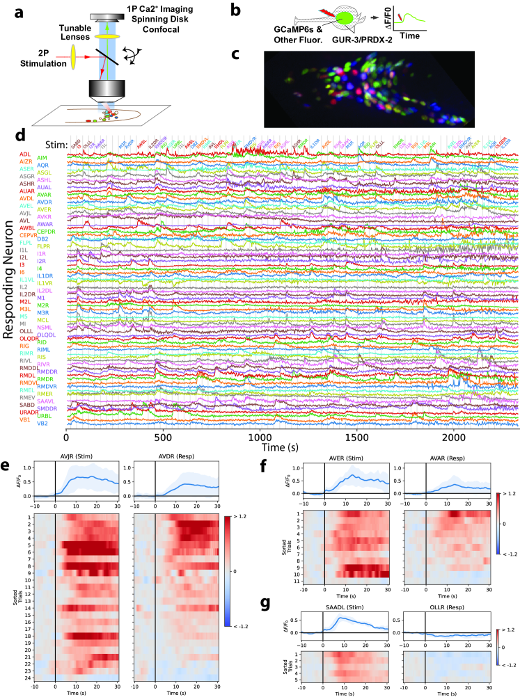
Figure 1: Measuring neural activation and network response. Schematics of a) the instrument and b) of the experiment. c) NeuroPAL fluorophores for neural identification. d) Whole-brain cell-resolved calcium activity (GCaMP6s fluorescence normalized by noise) during stimulation of individual neurons (gray vertical lines, listed at the top). e) Paired activity of AVJR and AVDR in response to AVJR stimulation, shown as relative change $\Delta F/F_{0}$. Top panel: average (blue) and standard deviation (shading) across trials and animals. Bottom panel: simultaneously recorded paired activity for individual trials (sorted by mean AVDR activity). All trials are shown that elicitced activity. f) Same as e for AVER stimulation and AVAR response. g) Same as e for SAADL stimulation and OLLR response.

To measure signal propagation, we activated each single neuron, one at a time, while simultaneously recording population calcium activity at cellular resolution. We recorded activity from 113 wild-type (WT) background animals, each for up to 40 min, while stimulating a mostly-randomly selected sequence of neurons one-by-one every 30 s (Fig. 1). We combined whole-brain calcium imaging via spinning disk single-photon confocal microscopy [48, 49] with two-photon [50] targeted optogenetic stimulation [51], each with their own remote focusing system, to measure and manipulate neural activity in an immobilized animal (Fig. 1a). Animals were awake and pharyngeal pumping was visible during recordings. We spatially restricted the optogenetic excitation volume in three dimensions to the typical size of a C. elegans cell soma (Extended Data Fig. 2a) using temporal focusing [52, 43] to address single neurons without also activating their neighbors (Extended Data Figs. 2c,d).

To overcome challenges associated with spectral overlap [43, 44, 53, 54, 55], we expressed the GUR-3/PRDX-2 purple-light activatable optogenetic system [56, 57] and a nuclear-localized calcium indicator GCaMP6s [58] in each neuron (Fig. 1b). Light activation of GUR-3 had previously been shown to elicit both calcium responses and behavioral responses. For example, light-activation of GUR-3 in I2 was shown to inhibit pharyngeal pumping by release of glutamate [59]. Light activation of GUR-3/PRDX-2 expressed in AVA evoked reversals (Extended Data Fig. 2h), as expected [60, 61]. To obtain high expression levels of GUR-3/PRDX-2 with less toxicity we expressed it under the control of a drug-inducible gene expression system and only turned on gene expression prior to experiments. The stimulus illumination duration of 0.3 s or 0.5 s was chosen to evoke modest amplitude calcium responses (Extended Data Fig. 2f), similar in amplitude to those evoked by natural odor stimuli [62]. Activation of cholinergic motor neurons M1 under these stimulation conditions evoked pharyngeal muscle contraction (Supplementary Video 1). This provides evidence that our stimulation condition is well suited to evoke typical synaptic release of classical neurotransmitters, since M1 is known to release acetylcholine via chemical synapse onto pharyngeal muscles [63, 64].

We performed calcium imaging, with excitation light at a wavelength and intensity that does not elicit photoactivation of GUR-3/PRDX-2 (Extended Data Fig. 2b) [65]. We also used genetically encoded fluorophores from NeuroPAL expressed in each neuron [66] to identify neurons consistently across animals (Fig. 1c). Many neurons exhibited calcium activity in response to activation of one or more other neurons (Fig. 1d). A downstream neuron’s response to a stimulated neuron is evidence that a signal propagated from the stimulated neuron to the downstream neuron.

We highlight three examples from the motor circuit (Fig. 1e-g). Stimulation of the interneuron AVJR evoked activity in AVDR (Fig. 1e). AVJ had been predicted to coordinate locomotion upon egg laying by promoting forward movements [67]. AVD activity is associated with sensory-evoked (but not spontaneous) backward locomotion [19, 68, 20, 69] and receives chemical and electrical synaptic input from AVJ [70, 12]. Both the wiring and our functional measurements suggest that AVJ may also play a role in coordinating backward locomotion, in addition to its previously described roles related to egg laying and forward locomotion.

Activation of premotor interneuron AVE evoked activity transients in AVA (Fig. 1f). Both AVA [71, 47, 72, 69, 73, 74, 75, 76] (Extended Data Fig. 2h) and AVE [69, 75] are implicated in backward movement and have activity correlated with one another [69] and AVE makes gap junction and many chemical synaptic contacts with AVA [70, 12].

Activation of the turning-associated neuron SAADL [75] inhibited activity in sensory neuron OLLR. SAAD had been predicted to inhibit OLL based on gene expression measurements [77]. SAAD is cholinergic and it makes chemical synapses to OLL which expresses an acetylcholine-gated chloride channel, LGC-47 [78, 79, 12].

Selected additional neural responses that are consistent with previous reports in the literature are listed in Extended Data Fig. 10.

Signal propagation map

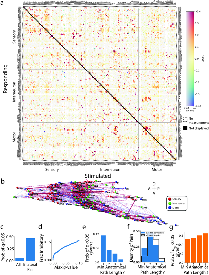
Figure 2: Signal propagation map of C. elegans. a) Mean post-stimulus neural activity $\langle\Delta F/F_{0}\rangle_{t}$ averaged across trials and individuals. $q$-values report false discovery rate (more gray is less significant). White indicates no measurement. Auto-response is required for inclusion and not displayed (black diagonal). $N$=113 animals. Neurons that were recorded but never stimulated are shown in Extended Data Fig. 5. b) Corresponding network graph with neurons positioned anatomically (only $q<0.05$ connections). Width and transparency indicate mean response amplitude (red, excitatory; blue, inhibitory). c) A bilaterally symmetric pair is more likely to have a $q<0.05$ functional connection than a pair chosen at random. d) Fraction of connections that are inhibitory as a function of the $q$-value threshold. Green indicates $q<0.05$. e) Probability of being functionally connected ($q<0.05$) given minimum anatomical path length $l$. f) Distribution of $l$ for functionally connected pairs (blue) compared to all possible pairs (black). g) Probability of being functionally non-connected ($q_{\mathrm{eq}}<0.05$) given $l$.

We generated a signal propagation map by aggregating downstream responses to stimulation for each neuron pair across recordings from 113 individuals (Fig. 2a). We report the average calcium response in a time window $\langle\Delta F/F_{0}\rangle_{t}$ averaged across trials and animals (Extended Data Fig. 3a). We imaged activity in response to stimulation for 23,427 neuron pairs (66% of all possible pairs in the head) at least once, and as many as 59 times (Extended Data Fig. 4a). This includes activity from 186 of 188 neurons in the head (99% of all head neurons, Extended Data Fig. 3b).

We employed two statistical tests to identify neuron pairs that are “functionally connected,” ‘functionally non-connected” or for which we lack confidence to make either determination. Both tests compare observed calcium transients in each downstream neuron to a null distribution of transients recorded in experiments lacking stimulation. To test whether a neuron pair is functionally connected, we seek to reject the null hypothesis that its downstream calcium transients could have arisen from the null distribution. We report a $q$-value, related to significance, that conveys the false-discovery rate across the many hypotheses tested in our large dataset[80, 81] (Extended Data Fig. 4b). Pairs that achieve $q<0.05$ are deemed “functionally connected.” To test whether a neuron pair is functionally non-connected, we perform a separate, equivalence test that seeks to reject the null hypothesis that the effect size of the observed transient is larger than some small $\epsilon$. Here too we report a false discovery rate, $q_{\mathrm{eq}}$ (Extended Data Fig. 5b). Neuron pairs with $q_{\mathrm{eq}}<0.05$ are declared functionally non-connected.

We emphasize that this statistical framework is conservative and presents a very high bar for which to declare a neuron pair to be functionally connected or functionally non-connected. Passing either of these hurdles requires consistent and reliable responses (or non-responses) and takes into account effect size, sample size, and multiple hypothesis testing. The majority of neuron pairs we measure fail to pass either of these tests, even though they often contain neural activity that, when observed in isolation, could easily be classified as a response (e.g. AVJR->ASGR in Extended Data Fig. 4c).

Our signal propagation map comprises the response amplitude and its associated $q$-value (Fig. 2a, Extended Data Fig. 5a). This functional dataset, overlaid on the anatomical wiring diagram [70, 12], is browseable online (https://funconn.princeton.edu) via software built on the NemaNode platform [12]. We estimate that at least 1,314 of the 23,427 measured neuron pairs, or 6 %, pass our stringent criteria to be deemed functionally connected at $q<0.05$ (Fig. 2c). We also mapped our confidence in neuron pairs that are functionally non-connected (Extended Data Fig. 5b). Note that in all cases functional connections refer to “effective connections” because they represent the propagation of signals over all paths in the network between the stimulated and responding neuron, not just the direct (monosynaptic) connections between them.

C. elegans neuron subtypes typically consist of two bilaterally symmetric neurons, often connected by gap junctions, that have similar neural wiring [70], similar gene expression [78], and correlated activity [82]. Our measurements show that bilaterally symmetric neurons are eight times more likely to be functionally connected than pairs of neurons chosen at random (Fig. 2c).

The balance of excitation and inhibition is important for a network’s stability [83, 84] but until now has not been directly measured in the worm. We measure that 11 % of $q<0.05$ functional connections are inhibitory (Fig. 2d), comparable to prior estimates of $\approx 20\%$ of synaptic contacts in C. elegans [77] or $\approx 20\%$ of cells in mammalian cortex [85]. Our estimate is likely a lower bound, because we assume that we only observe inhibition in neurons that already have tonic activity.

Neurons with a single-hop anatomical connection were more likely to be functionally connected at $q<0.05$ compared to neurons with only indirect or multi-hop anatomical connections; and functional connections became less likely as the minimal path length through the anatomical network increased (Fig. 2e). Conversely, neurons that had large minimal path-lengths through the anatomical network were more likely to be functionally non-connected than neurons that had a single-hop minimal path length (Fig. 2g). We investigated how far responses to neural stimulation penetrate into the anatomical network. Functionally connected ($q<0.05$) neurons were on average connected by a minimal anatomical path length of 2.1 hops (Fig. 2f), suggesting that neural perturbations often propagate multiple hops through the anatomical network or that neurons are also signaling directly through non-wired means, as explored later.

We observed instances of two types of variability in neural responses across trials and individuals: (1) a downstream neuron responds to stimulation of a given upstream neuron in only some simulations but not others (Extended Data Fig. 6a) and (2) the amplitude, temporal shape, and sign of the response varies from one stimulation to the next (Extended Data Fig. 6b-e). Some variability in the responding neuron’s activity can be attributed to variability of the upstream neuron’s activity. (We refer to a neuron’s response to its own stimulation as an auto-response.) To study variability in the strength, temporal properties, and sign of the connection, while excluding variability contributed by the upstream neuron’s activity, we calculated a kernel for each stimulation that caused a response. The kernel gives the activity of the downstream neuron when convolved with the activity of the upstream neuron. The kernel describes how the signal is transformed from upstream to downstream neuron for that stimulus event, including the timescales of the signal transfer (Extended Data Fig. 6b,c). We characterized variability of each functional connection by comparing how these kernels transform a standard stimulus (Extended Data Fig. 6e). Many neuron pairs had collections of kernels with properties that varied across trials. We did not identify the sources of this variability, but they likely include state- and history-dependent effects [60], including from neuromodulation [31, 86], plasticity, and inter-animal variability in wiring and expression. Collections of kernels within a neuron pair were more stereotyped than collections of kernels randomly selected from across shuffled pairs (Extended Data Fig. 6f), as expected.

Functional connectivity differs from anatomy

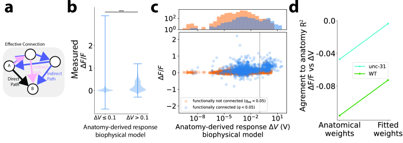
Figure 3: Functional connectivity differs from anatomy. a) Functional connectivity describes effective connections, which can include direct (black), indirect (pink), and recursive (purple) paths. Instead, anatomical features like synapse count describe only direct paths (black). To make a like-to-like comparison, anatomy-derived effective connections are computed in connectome-constrained simulations. b) Pairs predicted from anatomy to have large stimulus evoked downstream responses ($\Delta V>0.1V$) tend to have stronger measured responses (larger $\Delta F/F$ in the downstream neuron) than pairs that anatomy predicts to have small stimulus-evoked downstream responses. ($p<0.0001$, one-sided KS test). c) Main panel: Measured downstream response ($\Delta F/F$) vs. anatomy-derived response ($\Delta V$) for pairs that we observe to be functionally connected ($q<0.05$, blue) and functionally non-connected ($q_{\mathrm{eq}}<0.05$, orange). The vertical gray line is the threshold ($0.1V$) that separates anatomy-predicted effective connections from non-connections. Top panel: Marginal distributions (note y-axis is log scale). Functionally connected pairs are enriched for anatomy-predicted effective connections, compared to functionally non-connected pairs. ($p<0.0001$, one-sided KS test). d) Agreement of measured responses to anatomy-predicted responses is shown for wild-type (green) and unc-31 animals (cyan) in two conditions: using weights and signs from anatomy, or when weights and signs are fitted optimally. Agreement is calculated as the $R^{2}$ coefficient for the line-of-best-fit: $\Delta F/F=m\Delta V$. Perfect agreement would be $R^{2}=1$.

We sought to compare our measured functional connectivity to anatomy [70, 87, 12]. Functional connectivity and anatomical connectivity describe different levels of the network – functional connectivity measures effective connection between two neurons, including contributions from all paths through the network, direct and indirect (Fig. 3a). In contrast, anatomical features such as synapse count are properties of only the direct (monosynpatic) connection between two neurons. A bridge is needed between these two levels of description in order to make a like-to-like comparison. Therefore, we used connectome-constrained biophysical models of the network to simulate the expected signal propagation based on anatomy. We activated neurons in silico and simulated the network’s response, using synaptic weights from anatomy [70, 12], synaptic polarities estimated from gene expression [77], and using common assumptions about timescales and dynamics [88].

The anatomy-derived biophysical model made some predictions that agreed with our functional measurements. We classified neuron pairs into anatomy-predicted effective connections or anatomy-predicted effective non-connections based on the biophysical model (threshold of $\Delta V=0.1$). Anatomy-predicted effective connections were significantly more likely to correspond to larger amplitude responses in our measurements than predicted non-connections (Fig. 3b), showing agreement between structure and function. Similarly, we find that functionally connected pairs of neurons ($q<0.05$) are relatively enriched for anatomy-predicted effective connections compared to functionally non-connected neurons ($q_{\mathrm{eq}}<0.05$), (Fig. 3c, top panel).

Overall, however, there was fairly poor agreement between anatomical predictions and measurement. For example, we measured non-zero responses in neuron pairs that were predicted from anatomy to have almost no response (Fig. 3c). The agreement between anatomy predicted and measured response was also poor when considering all neuron pairs (Fig. 3d, $R^{2}$<0, where an $R^{2}$ of 1 would indicate perfect agreement).

It is challenging to infer the strength, sign or other functional properties of a neural connection from anatomy and this may contribute to the disagreement between anatomical predictions and our measurements. In mammals [25] and worms [77] presynaptic neurons can send both excitatory and inhibitory signals to their postsynaptic partner leaving the overall strength and sign ambiguous. For example, the AFD-AIY pair expresses machinery for inhibition via glutamate but we and others find it to be functionally excitatory likely due to peptidergic signaling [89] (Extended Data Fig. 2g). ASE-AIB is another ambiguous pair reported in the literature [90].

We therefore wondered whether agreement between structure and function would improve if we allowed the strength and signs of our biophysical model to float, but forbade the creation of entirely new connections that hadn’t appeared in the connectome. We fit strength and sign in the biophysical model from information about the measured effective functional connections. For simplicity during fitting, we assumed a linear network at steady state, but during the comparison we relaxed this assumption. Allowing the anatomical weights and signs to change in the most favorable way –but without adding any new connections – improved agreement between the anatomical prediction and functional measurements, although overall agreement remained poor (Fig. 3d).

We therefore explored whether additional functional connections exist that are not present in the anatomical wiring. We measured signal propagation in unc-31 mutant animal defective for dense-core vesicle-mediated extrasynaptic signaling, as explained below. While agreement was still poor, the signal propagation in these animals showed better agreement with anatomy than for WT (Fig. 3d). This prompted us to explore extrasynaptic signaling further.

Extrasynaptic signaling also drives neural dynamics

Neurons can communicate extrasynaptically by releasing transmitter that binds to receptors of downstream neurons after diffusing through the extracellular milieu instead of directly traversing a synaptic cleft. Such extrasynaptic signaling, sometimes called “volume transmission” [91], occurs either because the transmitter is released far from the cleft, for example via dense core vesicle, or because transmitter released at the cleft spills out into the milieu. Extrasynaptic signaling has been reported for GABA [92, 93], NMDA [94], monoamines [34], and neuropeptides [95]. In all cases, extrasynaptic signaling is not visible from anatomy and therefore forms additional wireless layers of communication in the nervous system [34]. We are motivated to investigate extrasyaptic signaling of neuropeptides in particular because neuropeptides and neuropeptide receptors are ubiquitous across not only the C. elegans nervous system [78, 96, 97] but also in mammalian cortex [98]. Neuropeptides are typically released via dense core vesicles [99] and are not required to be released at the synaptic cleft. Here we refer to dense-core-vesicle mediated signaling as extrasynaptic because it is commonly observed far from the synapse, however we cannot exclude the possibility that dense-core vesicles may also be released at the synapse.

To probe the role of dense-core mediated extrasynaptic signaling we measured a signal propagation map of unc-31-mutant animals defective for dense-core vesicle-mediated release (Extended Data Fig. 7a, 18 individuals) and compared their neural responses to WT animals. This mutant disrupts dense-core vesicle-mediated extrasynaptic signaling of peptides and monoamines because it lacks the UNC-31/CAPS protein that is involved in dense core vesicle fusion. In C. elegans, defects in UNC-31/CAPS are not expected to disrupt chemical or electrical synapses [100]. The signal propagation map of this mutant is browseable online and can be compared to WT at https://funconn.princeton.edu.

Extrasynaptic signaling is often associated with neuromodulation and is assumed to alter excitability or modulate synaptic properties that change how neurons respond to inputs [31, 95] often over long timescales, though not always [101]. But extrasynpatic transmission can also directly evoke activity in downstream neurons. Our signal propagation measurements are not designed to directly detect changes to a neuron’s excitability and instead such changes might appear as variability in our measured responses. But our measurements should detect instances where extrasynaptic signaling evokes activity.

Many functional connections remain in the unc-31 mutant, consistent with our expectation that chemical synapse and gap-junction mediated signaling plays a prominent role in the nervous system (Extended Data Fig. 8). For neuron pairs observed in both WT and unc-31 mutants, unc-31 animals had a smaller proportion of high-confidence functional connections (Extended Data Fig. 7b), consistent with the expected loss of extrasynaptic unc-31-dependent signaling between neurons.

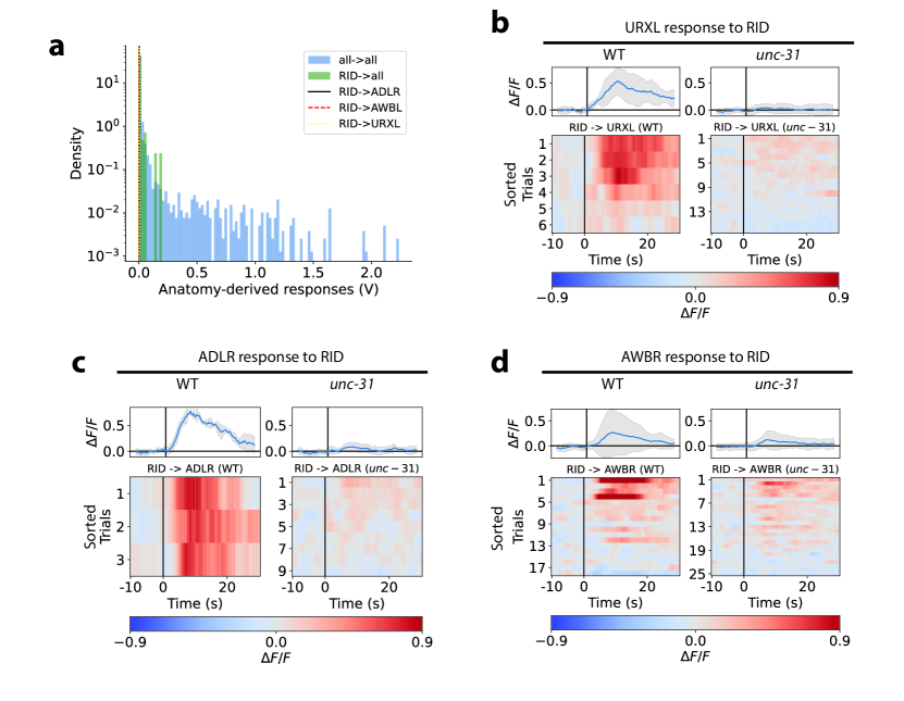
Figure 4: Anatomy omits extrasynaptic signaling from neuron RID. a) ADL, AWB, and URX are among the neurons predicted from anatomy to have no response to RID stimulation because there is no strong anatomical path from RID to those neurons (vertical lines at or near 0 volts). Their RID-evoked anatomy-predicted responses are shown within the distribution of anatomy-predicted responses for all neuron pairs (blue histogram), as in Fig. 3b. b-d.) Activity of neurons b) URXL, c) ADLR, and d) AWBR to RID stimulation, in WT and unc-31 mutant backgrounds. Top panel: average across trials and animals. Bottom panel: individual traces are sorted across trial and animal by mean response amplitude. Here trials are shown even in cases when RID activity was not measured. Responses of additional neurons are shown in Extended Data Fig. 7c

We sought to investigate specific extrasynaptic connections because these connections contribute to discrepancies between an anatomical and functional description. We first turned to the neuron RID, a neuroendocrine-like cell that is thought to signal to other neurons extrasynaptically via neuropeptides such as FLP-14, PDF-1, and INS-17 [102, 78]. RID has many potential extrasynaptic signaling partners but only very few and weak outgoing wired connections making it a good candidate in which to observe extrasynaptic signaling. In our imaging strain, RID exhibited only dim tagRFP-T expression, which prevented us from consistently segmenting the neuron in order to capture RID’s own calcium response to activation. We nonetheless stimulated RID and observed other neurons’ responses (Extended Data Fig. 7c). For analysis of responses to RID activation in Extended Data Fig. 7c and Fig. 4a only, we have relaxed our inclusion requirements and include downstream neural responses even when we do not measure the calcium activity of RID.

We inspected the activity of three neuron subtypes, URX, ADL, and AWB, that were predicted to have little or no response to RID stimulation based on anatomy (Fig. 4a) but showed notably strong responses to RID stimulation when measured in WT background (Fig. 4b-d). Several lines of evidence led us to conclude that RID predominantly sends signals to URX, ADL and AWB extrasynaptically. (1) When RID was stimulated in the unc-31 background, these three neurons all exhibited reduced amplitude or were less likely to respond at all (Fig. 4b-d), suggesting that these neurons’ connections to RID are dense-core-vesicle-dependent. (2) All three neuronal subtypes express receptors for peptides produced by RID (NPR-4 and NPR-11 for FLP-14 and PDFR-1 for PDF-1). And (3) there are no direct (monosynaptic) connections through the anatomical network from RID to URX, ADL, or AWB. The shortest paths from RID to URXL or AWBR require two hops ($l=2$), and three hops for ADLR ($l=3$), and in each case they rely on fragile single-contact synapses that appear in only one out of the four individual connectomes [12]. Taken together, we conclude that RID signals to other neurons extrasynaptically and that this signalling is captured by our functional measurements but not by anatomy.

Figure 5: a) Candidate purely extrasynaptic-dependent connections. b) Distribution of kernel rise times, as in Extended Data Fig. 6d. c) Paired responses for M3L->URYVL and d) AVDR->AVDL, respectively, shown for WT and unc-31 animals. unc-31 animals do not show downstream responses to stimulation. AVDR->AVDL extrasynaptic communication is putatively mediated in autocrine loops via NLP-10->NPR-35 and FLP-6->FRPR-8 signaling.

A screen for purely extrasynaptic-dependent signal propagation

Neuron RID had already been identified in the literature as a neuroendocrine-like cell that likely communicates extrasynaptically [102]. To identify new pairs of neurons that are purely extrasynaptic-dependent, we performed an unbiased screen and selected for neuron pairs that had functional connections in wild-type animals ($q<0.05$) but were functionally non-connected in animals defective for extrasynaptic signaling ($q_{\mathrm{eq}}<0.05)$. Out of the 1,314 pairs that we are confident are functionally connected in WT animals ($q<0.05$), 53 met the stringent threshold of also being functionally non-connected in unc-31 animals (Fig. 5a, Extended Data Fig. 9. These putative purely extrasynaptic-dependent connections represent a conservative lower-bound on the number of purely extrasynaptic-dependent connections in the brain.

Notably the distribution of timescales of unc-31-mediated functional connections is similar to that of all functional connections, Fig. 5b.

Neuron pair M3L->URYVL is a representative example of a purely extrasynaptic-dependent connection found from our screen. There are no direct wired connections between M3L and URYVL, but stimulation of M3L evokes unc-31-dependent calcium activity in URYVL (Fig. 5c). The recent de-orphaniziation of many neuropeptide receptors [97], combined with gene expression data [78], provides candidate neuropeptide/GPCR combinations mediating the communication in the majority of neuron pairs we identify (listed in Supporting Spreadsheet 1). For example, M3L and URYVL express the following peptides and receptors, respectively, that can bind with one another: peptide FLP-4 binds to receptor NPR-4 and peptide FLP-5 binds to receptor NPR-11. Additional peptide/receptor pairs are also likely expressed, albeit at lower levels, as described in methods.

The screen identifies only those subset of neural connections for which signal propagation is completely absent in unc-31. Many more neuron pairs likely signal through multiple parallel paths including both synaptic and extrasynaptic ones, or exhibit co-transmission of both, and these would not appear in the screen. Given the degree of anatomical connectedness (any neuron is anatomically connected to any other in no more than four hops) it is striking that we found so many neuron pairs that pass our stringent test for purely extrasynaptic dependence. We note that pairs that pass our screen could include signaling paths that involve synaptic signaling in series with extrasynaptic signaling, as this would still be purely extrasynaptic dependent. Our screen assumes that the unc-31 mutant is defective only for dense core vesicle release, as reported [100]. Defects in any additional signaling modes, or changes to wiring, would present a confound to interpreting these measurements.

We found bilateral partners among the candidate pairs of neurons identified in our screen for having purely extrasynaptic-dependent connections. These bilateral partners typically had no or only weak wired connections between them, and anatomy predicted very weak evoked responses (i.e. below the threshold displayed in Fig. 3b and c). AVDR and AVDL is the most prominent bilateral pair found in our screen. Stimulation of AVDR evoked robust unc-31-dependent responses in its bilateral partner AVDL. AVDR and AVDL have no or only weak wired connections between them (three of four connectomes show no wired connections, and the fourth finds only a very weak gap junction). Signal propagation between these bilateral partners is consistent with neuropeptidergic signaling, particularly via autocrine loops, in which a genetically defined cell sub-type expresses both a neuropeptide and the receptor to which it binds [96, 97]. The AVD cell-type was recently predicted to have a strong autocrine loop based on gene expression and peptide/GPCR interaction studies  [96] mediated by the neuropeptide/GPCR combinations NLP-10->NPR-35 and FLP-6->FRPR-8 [78, 97] (Fig. 5d). Moreover, AVD was predicted to be among the top 25 highest-degree “hub” nodes in a peptidergic network based on gene expression [96]. Consistent with this, we find that AVD is heavily represented among hits in our screen (Extended Data Fig 9b).

We note that the existence of a neuropeptide/GPCR combination indicates only that the molecular machinery for extrasynaptic peptidergic signaling is present. By contrast, functional measurements like those performed here provide the more direct evidence that extrasyanaptic signaling actually occurs. Moreover functional measurements resolve whether such signaling directly evokes neural responses, as in this case, or for example, whether they only modulate neural excitability over longer-timescales.

Signal-propagation better predicts spontaneous activity than anatomy

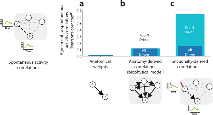
Figure 6: Measured signal-propagation better predicts spontaneous activity than anatomy. Schematic illustrates the types of measurements used to predict spontaneous activity correlations. a) Agreement (as Pearson’s correlation coefficient) between anatomical weights (synapse counts) and correlation matrix of spontaneous activity recorded from an immobilized animal. b) Agreement between correlations in anatomy-derived activity and those measured from spontaneous activity. Anatomy-derived activities and correlations are calculated in silico by driving all neurons (dark blue) or only an optimal subset of top-n neurons (light-blue). For anatomy, the optimal set is all neurons so the bars are the same. c) Agreement between correlations in spontaneous activity and correlations derived from functional measurements of signal propagation are reported. Functionally-derived correlations are calculated using measured signal-propagation kernels by either: driving all neurons (dark blue) or only an optimal subset, in this case the top 6 (light blue).

A key motivation for mapping neural connections is to understand how they give rise to neural dynamics. We therefore compared how well functional and anatomical descriptions of the network predict spontaneous neural activity. We measured the spontaneous network activity of immobilized worms without any optogenetic activators under bright imaging conditions, similar to [74], and compared correlations in the spontaneous activity to predictions from anatomy and from our signal propagation measurements (Fig. 6). We compared spontaneous activity to two different anatomical descriptions. First, we compared the matrix of spontaneous activity correlations to the matrix of the bare anatomical weights, or synapse counts between neurons, (Fig. 6a) which had previously been shown to have poor agreement [66, 82] and our experiments further support this conclusion. Poor agreement is unsurprising because descriptions of the monosynaptic contacts only captures direct connections between two neurons, while activity correlations are influenced by all possible paths through the network. We therefore also compared spontaneous correlations to anatomical predictions from the connectome-constrained biophysical model that considers all anatomical paths through the network. We drove activity in the biophysical model in silico and computed correlations from the resulting simulated activity. These anatomy-derived correlations showed better but still poor agreement with those measured in spontaneous activity (Fig. 6b).

We also compared spontaneous activity correlations to correlations predicted by our measurements of signal propagation (functionally-derived simulations). The functionally-derived correlations better predicted spontaneous activity than either of the anatomy-based approaches (Fig. 6c). To derive correlations from our signal propagation measurements we drove neurons in silico, propagated their activity through our measured kernels, and calculated the correlation matrix from the resulting activity.

We compared performance using two different assumptions: that all neurons drive spontaneous activity (“all driven”) or that only an optimal subset of neurons drive spontaneous activity (“top-$n$ driven”). To find the subset, we ranked-ordered each neuron’s individual agreement to spontaneous activity and selected the top-$n$ ranked neurons that collectively had the best agreement when driven.

Functionally-derived correlations based on signal propagation measurements always outperformed the anatomy-based correlations, but the performance is most significant under the assumption that the top-$n$ neurons are driven (Fig. 6c). Driving activity in the top 6 neurons dramatically improved agreement of the functionally-derived correlations to spontaneous activity compared to the all-driven assumption. Interestingly, for anatomy-derived correlations, we could not identify a top-n subset of neurons that significantly improved performance (Fig. 6b). Taken together, we conclude that functionally-derived predictions based on our signal propagation measurements better agree with spontaneous activity correlations than does anatomy, and that some subsets of neurons likely make outsized contributions to driving spontaneous dynamics.

Using our measured signal propagation kernels to simulate the worm’s neural activity has two distinct advantages compared to the anatomy-derived biophysical model and all other previous simulations of C. elegans: First, all of the parameters in the equations governing neural dynamics are extracted directly from the measured kernels that describe signal propagation: including the timescales, weights, signs, and connectivity, thereby avoiding ambiguities that arise from interpreting the connectome and transcriptome. Second, unlike all previous models that rely on the connectome, the functional measurements here capture extrasynaptic signaling, such as from neuropeptides, that likely contribute to spontaneous activity but are not visible in anatomy. These two advantages likely both contribute to why functional-derived predictions of correlations outperform anatomy at predicting spontaneous correlations. An interactive version of our functionally-derived simulation is available at https://funsim.princeton.edu.

Discussion

Signal propagation in C. elegans measured by neural activation differs from predictions based on anatomy in part because anatomy fails to account for wireless connections such as extrasynaptic release of neuropeptides [34]. We find that extrasynaptic signaling serves a functional role similar to that of classical neurotransmitters by directly evoking calcium activity on seconds timescale. We therefore conclude that extrasynaptic and synaptic signals together drive neural dynamics. The role of extrasynaptic signaling in directly evoking activity is likely in addition to its more well-characterized role in modulating neural excitability over longer-timescales of many minutes.

Our work complements recent efforts to map peptidergic signaling based on gene expression and neuropeptide/GPCR interaction studies [97, 96]. Gene expression can be used to identify pairs of neurons that express the correct peptides and receptors for signaling. But measurements of signal propagation, like those performed here, are needed to reveal whether signaling is actually present and to measure the temporal properties and functional role of signaling. In this work we provided a list of purely extrasynaptic-dependent connections that can be used to validate predictions based on gene-expression.

Peptidergic extrasynaptic signaling relies on diffusion and therefore C. elegans’ small size may be uniquely well-suited for this mode of signal propagation. Mammals express neuropeptides and receptors, including in multiple brain areas and throughout mouse cortex [98], but their larger brain size may limit the speed, strength or spatial extent of peptidergic extrasynaptic signaling.

Plasticity, neuromodulation, neural network state, and other longer-timescale effects may contribute to variability in our measured responses or to discrepancies between anatomical and functional descriptions of the C. elegans network. A future direction will be to search for latent connections that may only become functional in certain internal states.

Our signal propagation map provides a lower bound on the number of functional connections. Our analysis has fewer observations of neurons whose tagRFP-T expression is too dim or whose color and location pattern is too difficult to identify, and we are limited to calcium activity in the nucleus, and therefore omit compartmentalized calcium dynamics [103]. To better probe nonlinearities in the network, future measurements are needed that explore a larger stimulation space, including simultaneous stimulation of multiple neurons. Future work is also needed to probe functional connections in worms that are unrestrained and free to move.

Our signal propagation map reports effective connections, not direct connections. Effective connections are the most relevant and useful for answering the circuit-level questions that motivate our work, such as how a stimulus in one part of the network drives activity in another. By contrast, the properties of direct connections are well suited for probing questions of gene expression, development and anatomy, but can be less informative of network function. For example, a direct connection between two neurons may be slow or weak, but may overlook a fast and strong effective connection via other paths through the network. Here we have compared different network descriptions at the level of effective connections, in this case by using connectome-constrained simulations to derive effective connections from anatomy. An alternative approach would be to infer properties of direct connections from the measured effective connections, e.g. following [104], but solving this inverse problem may require a higher signal-to-noise ratio than our current measurements.

The neural dynamics we observe are slow but no slower than typical calcium responses to natural stimuli such as odor delivery [105]. The slow dynamics likely result from the slow graded potentials in C. elegans [89, 106], the slower calcium dynamics of the nucleus [74] and the slow rise and fall time of GCaMP6s [58] and GUR-3/PRDX-2 [56]. We identify fast signal transmission, even in slow dynamics, by fitting kernels to relate the dynamics of upstream and downstream neurons.

The signal propagation atlas presented here informs structure-function investigations at the level of both circuits and whole networks and also enables more accurate brain-wide simulations of neural dynamics and behavior. Crucially this work quantifies discrepancies between what is expected from anatomy and what is observed functionally at brain scale and cellular resolution for a complete connectome. The finding that extrasynaptic peptidergic signaling directly evokes activity and drives dynamics in C. elegans will inform ongoing discussion about efforts to characterize other brains at greater detail and scale.

Funding

Research reported in this work was supported by the National Institutes of Health National Institute of Neurological Disorders and Stroke under New Innovator award number DP2-NS116768 to AML; the Simons Foundation under award SCGB #543003 to A.M.L.; by the Swartz Foundation through the Swartz Fellowship for Theoretical Neuroscience to F.R.; by the National Science Foundation, through the Center for the Physics of Biological Function (PHY-1734030); and by the Boehringer Ingelheim Fonds to S.D. Strains from this work are being distributed by the CGC, which is funded by the NIH Office of Research Infrastructure Programs (P40 OD010440).

Author contributions

A.M.L. and F.R. conceived the experiments, F.R. and S.D. conducted the experiments, A.K.S. designed and performed all transgenics, F.R. designed and built the instrument and the analysis framework and pipeline, F.R. and S.D. performed the bulk of the analysis with additional contributions from A.M.L. and A.K.S. All authors wrote and reviewed the manuscript.

Data and materials availability

Data is available in an interactive and browseable format at https://funconn.princeton.edu and http://funsim.princeton.edu. Machine readable datasets are publicly accessible through on Open Science Foundation repository at https://osf.io/e2syt/. All analysis code is publicly available at https://github.com/leiferlab/pumpprobe, https://github.com/leiferlab/wormdatamodel, https://github.com/leiferlab/wormneuronsegmentation, and https://github.com/leiferlab/wormbrain. Hardware acquisition code is available at https://github.com/leiferlab/pump-probe-acquisition

Online Methods

Worm Maintenance

C. elegans were stored in the dark, and only minimal light was used when transferring worms or mounting worms for experiments. Strains generated in this study (Extended Data Fig. 1a) have been deposited in the Caenorhabditis Genetics Center, University of Minnesota, for public distribution.

Transgenics

To measure functional connectivity, we generated the transgenic strain AML462. This strain expresses the calcium indicator GCaMP6s in the nucleus of each neuron, a purple light-sensitive optogenetic protein system (i.e., GUR-3 and PRDX-2) in each neuron, and multiple fluorophores of various colors from the NeuroPAL[66] system also in the nucleus of neurons. We also used a QF-GR drug-inducible gene expression strategy to turn on gene expression of optogenetic actuators only later in development. To create this strain, we first generated an intermediate strain, AML456, by injecting a plasmid mix (75 ng/$\mu$l pAS3-5xQUAS::$\Delta$pes-10P::AI::gur-3G::unc-54 + 75 ng/$\mu$l pAS3-5xQUAS::$\Delta$pes-10P::AI::prdx-2G::unc-54 + 35 ng/$\mu$l pAS-3-rab-3P::AI::QF+GR::unc-54 + 100 ng/$\mu$l unc-122::GFP) into CZ20310 worms followed by UV integration and 6 outcrosses [107, 108]. The intermediate strain, AML456, was then crossed into the pan-neuronal GCaMP6s calcium imaging strain, with NeuroPAL, AML320 [66, 109].

An unc-31 mutant background with defects in the dense-core vesicle release pathway was used to diminish wireless signaling [100]. We created an unc-31 knockout version of our functional connectivity strain by performing CRISPR/Cas9-mediated genome editing on AML462 using a single-strand oligodeoxynucleotide (ssODN)-based homology-dependent repair strategy [110]. This approach resulted in strain AML508 (unc-31 [wtf502] IV; otIs669 [NeuroPAL] V 14x; wtfIs145 [pBX + rab-3::his-24::GCaMP6s::unc-54]; wtfIs348 [75 ng/$\mu$l pAS3-5xQUAS::$\Delta$pes-10P::AI::gur-3G::unc-54 + 75 ng/$\mu$l pAS3-5xQUAS::$\Delta$pes-10P::AI::prdx-2G::unc-54 + 35 ng/$\mu$l pAS-3-rab-3P::QF+GR::unc-54 + 100 ng/$\mu$l unc-122::GFP].

CRISPR/Cas-9 editing was carried out as follows. Protospacer adjacent motif (PAM) sites were selected in the first intron (gagcuucgcaauguugacucCGG) and the last intron (augguacauuggguccguggCGG) of the unc-31 gene (ZK897.1a.1) to delete 12,476 out of 13,169 bp (including the 5’ and 3’ untranslated regions [UTRs]) and 18 out of 20 exons from the genomic locus, while adding 6 bp (GGTACC) for the Kpn-I restriction site (Extended Data Fig. 1b). Alt-R S.p. Cas9 Nuclease V3, Alt-R-single guide RNA (sgRNA), and Alt-R homology-directed repair (HDR)-ODN were used (IDT, USA). We introduced the Kpn-I restriction site (gacccagcgaagcaaggatattgaaaacataagtacccttgttgttgtgtGGTACCccacggacccaatgtaccatattttacgagaaatttataatgttcagg) into our repair oligo to screen and confirm the deletion by PCR followed by restriction digestion. sgRNA and HDR ssODNs were also synthesized for the dpy-10 gene as a reporter, as described in [110]. An injection mix was prepared by sequentially adding Alt-R S.p. Cas9 Nuclease V3 (1 $\mu$L of 10 $\mu$g/$\mu$L), 0.25 $\mu$L of 1M KCL, 0.375 $\mu$L of 200 mM HEPES (pH 7.4), sgRNAs for unc-31 [1 $\mu$L each for both sites], and 0.75 $\mu$L for dpy-10 from a stock of 100 $\mu$M, ssODNs [1 $\mu$L for unc-31 and 0.5 $\mu$L for dpy-10 from a stock of 25 $\mu$M], and nuclease-free water to a final volume of 10 $\mu$L in a PCR tube, kept on ice. The injection mix was then incubated at 37 °C for 15 min before it was injected into the germline of AML462 worms. Progenies from plates showing roller or dumpy phenotypes in the F1 generation post-injection were individually propagated and PCR>Kpn-I digestion screened to confirm deletion. Single-worm PCR was carried out using GXL-PRIME STAR taq-Polymerase (Takara Bio, USA) and the Kpn-1-HF restriction enzyme (NEB, USA). Worms without a roller or dumpy phenotype and homozygous for deletion were confirmed by Sanger sequencing fragment analysis.

To cross validate GUR-3/PRDX-2 evoked behavior responses, we generated the transgenic strain AML546 by injecting a plasmid mix (40 ng/$\mu$l pAS3-rig-3P::AI::gur-3G::SL2::tagRFP::unc-54 + 40 ng/$\mu$l pAS3-rig-3P::AI::prdx-2G::SL2::tagBFP::unc-54) into N2- worms to generate transient transgenic line expressing GUR-3/PRDX-2 in AVA neurons.

Cross-validation of GUR-3/PRDX-2 evoked behavior

Optogenetic activation of AVA neurons using traditional channelrhodopsins (e.g. Chrimson) leads to reversals [60, 61]. We used worms expressing GUR-3/PRDX-2 in AVA neurons (AML 564) to show that GUR-3/PRDX-2 elicits a similar behavioral response. We illuminated freely moving worms with blue light from an LED (peaked at 480 nm, $2.3mW/mm^{2}$) for 45 s. We compared the number of onsets of reversals in that period of time with a control in which only dim white light was present, as well with the results of the same assay performed on N2 worms. Animals with GUR-3/PRDX-2 in AVA (n=11 animals) exhibited more blue-light evoked reversals per minute than WT (n=8 animals) (Extended Data Fig. 2h).

Dexamethasone treatment

To increase expression of optogenetic proteins while avoiding toxicity during the animals’ early life development, a drug-inducible gene expression strategy was used. Dexamethasone (dex) activates QF-GR to temporally control the expression of downstream targets [111], in this case the optogenetic proteins in the functional connectivity imaging strains AML462 and AML508. Dex-NGM plates were prepared by adding 200 $\mu$M of dex in DMSO just before pouring the plate. For dex treatment, L2/L3 worms were transferred to overnight-seeded dex-NGM plates and further grown until worms were ready for imaging. Further details of the dex treatment are described below.

We prepared stock solution of 100 mM dex by dissolving 1 gram Dexamethasone (D1756, Sigma-Aldrich) in 25.5 ml DMSO (D8418, Sigma-Aldrich). Stocks were then filter sterilized, aliquoted, wrapped in foil to prevent light, and stored at -80 C until needed. 200 $\mu$M dex-NGM plates were made by adding 2 ml of 100 mM dex stock in 1 liter of NGM-agar media, while stirring, 5 minutes before pouring the plate. Dex-plates were stored at 4 C for up to a month until needed.

Preparation of worms for imaging

Worms were individually mounted on 10 % agarose pads prepared with M9 buffer and immobilized using 2 $\mu$l of 100 nm polystyrene beads solution and 2 $\mu$l of levamisole (500 $\mu$M stock). This concentration of levamisole, after dilution in the polystyrene bead solution and the agarose pad water, largely immobilized the worm while still allowing the worm to slightly move, especially before placing the coverslip. Pharyngeal pumping was observed during imaging.

Multi-channel imaging and neural identification

Volumetric, multi-channel imaging was performed to capture images of the following fluorophores in the Neuropal transgene: mtagBFP2, CyOFP1.5, tagRFP-T, and mNeptune2.5 [66]. Light downstream of the same spinning disk unit used for calcium imaging traveled on an alternative light path through channel-specific filters mounted on a mechanical filter wheel, while mechanical shutters alternated illumination with the respective lasers, similar to [109]. Channels were as follows: mtagBFP2 was imaged using a 405 nm laser and a Semrock FF01-440/40 emission filter; CyOFP1.5 was imaged using a 505 nm laser and a Semrock 609/54 emission filter; tagRFP-T was imaged using a 561 nm laser and a Semrock 609/54 nm emission filter; and mNeptune2.5 was imaged using a 561 nm laser and a Semrock 732/68 nm emission filter.

After the functional connectivity recording was complete, a human manually assigned neuron identities by comparing each neuron’s color, position, and size to a known atlas. Some neurons are particularly hard to identify in NeuroPAL and are therefore absent or less frequently identified in our recordings. Some neurons have dim tagRFP-T expression, which makes it difficult for the neuron segmentation algorithm to find them and, therefore, to extract their calcium activity. These neurons include, for example, AVB, ADF, and RID. RID’s distinctive position and its expression of CyOFP allowed us nevertheless to manually target it optogenetically. Neurons in the ventral ganglion are hard to identify because it appears as very crowded when viewed in the most common orientation that worms assume when mounted on a microscope slide. Neurons in the ventral ganglion are therefore sometimes difficult to distinguish one from another, especially for dimmer neurons such as the SIA, SIB, and RMF neurons. In our strain, the neurons AWCon and AWCoff were difficult to tell apart based on color information.

Volumetric image acquisition

Neural activity was recorded at whole-brain scale and cellular resolution via continuous acquisition of volumetric images in red and green channels with a spinning disk confocal unit and via LabView software (https://github.com/leiferlab/pump-probe-acquisition/tree/pp), similarly to [112], with a few upgrades. The imaging focal plane was scanned through the brain of the worm remotely using an electrically tunable lens (Optotune EL-16-40-TC) instead of moving the objective. The use of remote focusing allowed us to decouple the z-position of the imaging focal plane and that of the optogenetics 2-photon spot (described below).

Images were acquired by an sCMOS camera, and each acquired image frame was associated to the focal length of the tunable lens (z-position in the sample) at which it was acquired. To ensure the correct association between frames and z-position, we recorded the analog signal describing the focal length of the tunable lens at time points synchronous with a trigger pulse output by the camera. By counting the camera triggers from the start of the recording, the z-positions could be associated to the correct frame, bypassing unknown operating-system-mediated latencies between the image stream from the camera and acquisition of analog signals.

Additionally, real-time “pseudo”-segmentation of the neurons (described below) required the ability to separate frames into corresponding volumetric images in real-time. Because the z-position was acquired at low sample rate, splitting of volumes based on finite differences between successive z-positions could lead to errors in assignment at the edge of the z-scan. An analog OP-AMP-based differentiator was used to independently detect the direction of the z-scan in hardware.

Calcium imaging

Calcium imaging was performed in single-photon regime with a 505 nm excitation laser via spinning disk confocal microscopy, at 2 vol/s. For functional connectivity experiments, an intensity of 1.4 mW/mm² at the sample plane was used to image GCaMP6s, well below the threshold needed to excite the GUR-3/PRDX-2 optogenetic system [56]. We note that at this wavelength and intensity animals exhibited very little spontaneous calcium activity.

For certain analyses (Fig. 6), recordings with ample spontaneous activity were desired. In those cases, we increased the 505 nm intensity seven-fold to approximately 10 mW/mm² and recorded from AML320 strains that lacked exogenous GUR-3/PRDX-2 to avoid potential widespread neural activation. Under these imaging conditions, we observed population-wide slow stereotyped spontaneous oscillatory calcium dynamics, as previously reported [74, 113].

Extraction of calcium activity from the images

The extraction of calcium activity from the raw images was performed using Python libraries implementing optimized versions of the algorithm described in [114], available at https://www.github.com/leiferlab/pumpprobe,
https://www.github.com/leiferlab/wormdatamodel,
https://www.github.com/leiferlab/wormneuronsegmentation-c,
and https://www.github.com/leiferlab/wormbrain.

The positions of neurons in each acquired volume was determined by computer vision software implemented in C++. This software was greatly optimized to identify neurons in real-time in order to also enable closed-loop targeting and stimulus delivery (as described in the section Stimulus delivery and pulsed laser). Two design choices made this algorithm dramatically faster than previous approaches. First, a local maxima search was used instead of a slower watershed-type segmentation. The nuclei of C. elegans neurons are approximately spheres and so they can be identified and separated by a simple local maxima search. Second, we factorized the 3D local maxima search into multiple 2D local maxima searches. In fact, any local maximum in a 3D image is also a local maximum in the 2D image in which it is located. Local maxima were therefore first found in each 2D image separately, and then candidate local maxima were discarded or retained by comparing them to their immediate surroundings in the other planes. This makes the algorithm less computationally intensive and fast enough to be used also in real time. We refer to this type of algorithm as “pseudo”-segmentation because it finds the center of neurons without fully describing the extent and boundaries of each neuron.

After neural locations were found in each of the volumetric images, a nonrigid pointset registration algorithm was used to track their locations across time, matching neurons identified in a given 3D image to the neurons identified in a 3D image chosen as reference. Even worms that are mechanically immobilized still move slightly and contract their pharynx, thereby deforming their brain and requiring the tracking of neurons. We implemented in C++ a fast and optimized version of the Dirichelet-Student-t Mixture Model (DSMM)  [115].

Calcium pre-processing

The GCaMP6s intensity extracted from the images undergoes the following pre-processing steps. (1) Missing values are interpolated based on neighboring time points. Missing values can occur when a neuron cannot be identified in a given volumetric image. (2) Photobleaching is removed by fitting a double exponential to the baseline signal. (3) Outliers more than 5 standard deviations away from the average are removed from each trace. (4) Traces are smoothed via a causal polynomial filtering with a window size of 6.5 s and polynomial order of 1 [Savitzky–Golay filters with windows completely “in the past”, e.g., obtained with scipy.signal.savgol_coeffs(window_length=13,
polyorder=1, pos=12)]. This type of filter with the chosen parameters is able to remove noise without smearing the traces in time. Note that when fits are performed (e.g., to calculate kernels), they are always performed on the original, non-smoothed traces. (5) Where $\Delta F/F_{0}$ of responses is used, $F_{0}$ is defined as the value of $F$ in a short interval before the stimulation time.

Stimulus delivery and pulsed laser

For two-photon optogenetic targeting, we used an optical parametric amplifier (OPA, Light Conversion ORPHEUS) pumped by a femtosecond amplified laser (Light Conversion PHAROS). The output of the OPA was tuned to a wavelength of 850 nm, at a 500 kHz repetition rate. We used temporal focusing to spatially restrict the size of the 2-photon excitation spot along the microscope axis. A motorized iris was used to set its lateral size. For temporal focusing, the first-order diffraction from a reflective grating, oriented orthogonally to the microscope axis, was collected (as in [116]) and traveled through the motorized iris, placed on a plane conjugate to the grating. To arbitrarily position the 2-photon excitation spot in the sample volume, the beam then traveled through an electrically tunable lens (Optotune EL-16-40-TC, on a plane conjugate to the objective), to set its position along the microscope axis, and finally was reflected by two galvo-mirrors to set its lateral position. The pulsed beam was then combined with the imaging light path by a dichroic mirror immediately before entering the back of the objective.

The majority of the stimuli were delivered automatically by computer control. Real-time computer vision software found the position of the neurons for each volumetric image acquired, using only the tagRFP-T channel. To find neural positions, we used the same “pseudo”-segmentation algorithm described above. The algorithm found neurons in each 2D frame in $\sim$500 $\mu$s as the frames arrived from the camera. In this way locations for all neurons in a volume were found within a few milliseconds of acquiring the last frame of that volume.

Every 30 s, a random neuron was selected among the neurons found in the current volumetric image based only on its tag-RFP-T signal. After galvo-mirrors and tunable lens set the position of the 2-photon spot on that neuron, a 500 ms (300 ms for the unc-31 mutant strain) train of light pulses was used to optogenetically stimulate that neuron. The duration of stimulus illumination for the unc-31 mutant strain was selected to elicit calcium transients in stimulated neurons with a distribution of amplitudes such that the maximum amplitude was similar to those in WT background animals, (Extended Data Fig. 2f). The output of the laser was controlled via the external interface to its built-in pulse picker, and the power of the laser at the sample was 1.2 mW at 500 kHz. Neuron identities were assigned to stimulated neurons after the completion of experiments using NeuroPAL [66].

To probe the AFD-AIY neural connection, a small set of stimuli used variable pulse durations from 100 ms to 500 ms in steps of 50 ms selected randomly to vary the amount of optogenetic activation of AFD.

In some cases, neurons of interest were too dim to be detected by the real-time software. For those neurons of interest, additional recordings were performed in which a human manually selected the neuron to be stimulated based on its color, size, and position. This was the case for certain stimulations of neurons RID and AFD.

Characterization of the 2-photon excitation spot size

The lateral (xy) size of the 2-photon excitation spot was measured with a fluorescent microscope slide, while the axial (z) size was measured using 0.2 nm fluorescent beads (Suncoast Yellow, Bangs Laboratories), by scanning the z-position of the optogenetic spot while maintaining the imaging focal plane fixed (Extended Data Fig. 2a).

We further tested our targeted stimulation in two ways: selective photobleaching and neuronal activation. First, we targeted individual neurons at various depth in the worm’s brain, and we illuminated them with the pulsed laser to induce selective photobleaching of tagRFP-T. Extended Data Fig. 2c,d shows how our 2-photon excitation spot selectively targets individual neurons, because it photobleaches tagRFP-T only in the neuron that we decide to target, and not in nearby neurons. To faithfully characterize the spot size, we set the laser power such that the 2-photon interaction probability profile of the excitation spot would not saturate the 2-photon absorption probability of tagRFP-T. Second, we showed that our excitation spot is restricted along the z-axis by targeting a neuron and observing its calcium activity. When the excitation was directed at the neuron but shifted by 4 $\mu$m along z, the neuron showed no activation. In contrast, the neuron showed activation when the spot was correctly positioned on the neuron (Extended Data Fig. 2e).

Inclusion criteria

Stimulation events were included for further analysis if they evoked a detectable calcium response in the stimulated neuron. A classifier determined whether the response was detected by inspecting whether the amplitude of the $\Delta F/F_{0}$ transient and its second derivative exceeded hand-tuned thresholds. Stimulation events that did not meet this threshold were excluded. RID responses shown in Fig. 4 and Extended Data Fig. 7c are an exception to this policy. RID is visible based on its CyOFP expression, but its tagRFP-T expression is too dim to consistently extract calcium signals. Therefore in Fig. 4 and Extended Data Fig. 7c (but not in other figures, like Fig. 2) responses to RID stimulation were included even in cases where it was not possible to extract a calcium-activity trace in RID.

Neuron traces were excluded from analysis if a human was unable to assign an identity or if the imaging time points were absent in a contiguous segment longer than 5% of the response window due to imaging artifacts or tracking errors. A different policy applies to dim neurons of interest that are not automatically detected by the “pseudo”-segmentation algorithm in the 3D image used as reference for the pointset registration algorithm. In those cases, we manually added the position of those neurons to the reference 3D image. If these “added” neurons are automatically detected in most of the other 3D images, then a calcium activity trace can be successfully produced by the DSMM nonrigid registration algorithm and is treated as any other trace. However, if the “added” neurons are too dim to be detected also in the other 3D images and the calcium activity trace cannot be formed for more than 50% of the total time points, the activity trace for those neurons is extracted from the neuron’s position as determined from the position of neighboring neurons. In the analysis code, we refer to these as “matchless” traces, because the reference neuron is not matched to any detected neuron in the specific 3D image, but its position is just transformed according to the DSMM nonrigid deformation field. In this way, we are able to recover the calcium activity also of some neurons whose tag-RFP-T expression is otherwise too dim to be reliably detected by the “pseudo”-segmentation algorithm. Responses to RID stimulation shown in Fig. 4 and Extended Data Fig. 7c are an exception to this policy. There, the activity of any neuron for which there is not a trace for more than 50% of the time points is substituted with the corresponding “matchless” trace, and not just for the manually added neurons. This is important to be able to show responses of neurons like ADL, which have dim tagRFP-T expression. In this RID-specific case, in order to exclude responses that become very large solely because of numerical issues in the division by the baseline activity due to the dim tagRFP-T, we additionally introduce a threshold at $\Delta F/F=2$.

Kernels were computed only for stimulation-response events for which the automatic classifier detected responses in both the stimulated and downstream neurons. If the downstream neuron did not show a response, we considered the downstream response to be below the noise level and the kernel to be zero.

Statistical analysis

To assess the relative significance of a functional connection between a target and putative responding neuron, we calculated the probability of observing the measured calcium response given no neural stimulation. We used a two-sided Kolmogorov–Smirnov test to compare the distributions of $\Delta F/F_{0}$ and its temporal second derivative from all observations of that neuron pair to the empirical null distributions from control recordings lacking stimulation. $p$-values were calculated separately for $\Delta F/F_{0}$ and its temporal second derivative, and then combined using Fischer’s method to report a single fused $p$-value for each neuron pair. Finally, to account for the large number of hypotheses tested, a false discovery rate was estimated. From the list of $p$-values, each neuron was assigned a $q$-value via the Storey–Tibshirani method [81]. $q$-values are interpreted as follows: when considering an ensemble of putative functional connections of $q$-values all less than or equal to $q_{c}$, approximately $q_{c}$ of those connections would have appeared in a recording that lacked any stimulation.

To explicitly test whether a pair of neurons are functionally not-connected, taking into account the amplitude of the response, their reliability, and the number of observations, we also computed equivalence $p_{\mathrm{eq}}$ and $q_{\mathrm{eq}}$-values. This asseses the confidence of a pair not being connected. We test whether our response is equivalent to what we would expect from our control distribution using the two one-sided t-tests (TOST) [117]. We computed $p_{\mathrm{eq}}$-values for $\Delta F/F_{0}$ and its temporal second derivative for a given pair being equivalent to the control distributions within an $\epsilon=1.2\sigma_{\Delta F/F_{0},\partial_{t}^{2}}$. Here, $\sigma_{\Delta F/F_{0},\partial_{t}^{2}}$ is the standard deviation of the corresponding control distribution. We then combined the two $p_{\mathrm{eq}}$-values into a single one with the Fisher method and computed $q_{\mathrm{eq}}$-values. Note that, differently from the regular $p$-values described above, the equivalence test relies on the arbitrary choice of $\epsilon$, which defines when we call two distributions equivalent. We chose a conservative value of $\epsilon=1.2\sigma$.

Measuring path length through the synaptic network

To find the minimum path length between neurons in the anatomical network topology, we proceeded iteratively. We started from the original binary connectome and computed the map of strictly 2-hop connections by looking for pairs of neurons that are not connected in the starting connectome (the actual anatomical connectome at the first step) but that are connected through a single intermediate neuron. To generate the strictly 3-hop connectome, we repeated this procedure using the binary connectome including direct and 2-hop connections, as the starting connectome. This process continued iteratively to generate the strictly n-hop connectome.

In the anatomical connectome (the starting connectome for the first step in the procedure above), a neuron was considered to be directly anatomically connected if the connectomes of any of the four L4 or adult individuals in [10] and [12] contained at least one synaptic contact between them. Note that this is a permissive description of anatomical connections as it considers even neurons with only a single synaptic contact in only one individual to be connected.

Fitting kernels

Kernels $k_{ij}(t)$ were defined as the functions to be convolved with the activity $\Delta F_{j}$ of the stimulated neuron to obtain the activity $\Delta F_{i}$ of a responding neuron $i$, such that $\Delta F_{i}(t)=\big{(}k_{ij}*\Delta F_{j}\big{)}(t)$. To fit kernels, each kernel $k(t)$ was parametrized as a sum of convolutions of decaying exponentials

$$k(t)=\sum\limits_{m}c_{m}\big{(}\theta(t)e^{-\gamma_{m,0}t}\big{)}*\big{(}\theta(t)e^{-\gamma_{m,1}t}\big{)}*...,$$ (1)

where the indices $i,j$ are omitted for clarity and $\theta$ is the Heaviside function. This parametrization is exact for linear systems, and works as a description of causal signal transmission also in nonlinear systems. Note that increasing the number of terms in the successive convolutions does not lead to overfitting, as would occur by increasing the degree of a polynomial. Overfitting could occur by increasing the number of terms in the sum, which in our fitting is constrained to be a maximum of 2. The presence of two terms in the sum allows the kernels to represent signal transmission with saturation (with $c_{0}$ and $c_{1}$ of opposite signs) and assume a fractional-derivative-like shape.

The convolutions are performed symbolically. The construction of kernels as in Eq. (1) starts from a symbolically stored, normalized decaying exponential kernel with a factor $A$, $A\gamma_{0}\theta(t)e^{-\gamma_{0}t}$. Convolutions with normalized exponentials $\gamma_{n}\theta(t)e^{-\gamma_{n}t}$ are performed sequentially and symbolically, taking advantage of the fact that successive convolutions of exponentials always produce a sum of functions in the form $\propto\theta(t)t^{n}e^{-\gamma t}$. Once rules are found to convolve an additional exponential with a function in that form, any number of successive convolution can be performed. These rules are as follows:

1. If the initial term is a simple exponential with a given factor (not necessarily just the normalization $\gamma$) $c_{i}\theta(t)e^{-\gamma_{i}t}$ and $\gamma_{i}\neq\gamma_{n}$, then the convolution is

   $$c_{i}\theta(t)e^{-\gamma_{i}t}*\gamma_{n}\theta(t)e^{-\gamma_{n}t}=c_{\mu}\theta(t)e^{-\gamma_{\mu}t}+c_{\nu}\theta(t)e^{-\gamma_{\nu}t},$$ (2)

   with $c_{\mu}=\frac{c_{i}\gamma_{n}}{\gamma_{n}-\gamma_{i}}$, $c_{\nu}=-\frac{c_{i}\gamma_{n}}{\gamma_{n}-\gamma_{i}}$, and $\gamma_{\mu}=\gamma_{i}$, $\gamma_{\nu}=\gamma_{n}$.

2. If the initial term is a simple exponential and $\gamma_{i}=\gamma_{n}$, then

   $$c_{i}\theta(t)e^{-\gamma_{i}t}*\gamma_{n}\theta(t)e^{-\gamma_{n}t}=c_{\mu}\theta(t)te^{-\gamma_{\mu}t},$$ (3)

   with $c_{\mu}=c_{i}\gamma_{i}$ and $\gamma_{\mu}=\gamma_{i}$.

3. If the initial term is a $c_{i}\theta(t)t^{n}e^{-\gamma_{i}t}$ term and $\gamma_{i}=\gamma_{\mu}$, then

   $$c_{i}\theta(t)t^{n}e^{-\gamma_{i}t}*\gamma_{n}\theta(t)e^{-\gamma_{n}t}=c_{\mu}\theta(t)t^{n+1}e^{-\gamma_{\mu}t},$$ (4)

   with $c_{\mu}=\frac{c_{i}\gamma_{i}}{n+1}$ and $\gamma_{\mu}=\gamma_{i}$.

4. If the initial term is a $c_{i}\theta(t)t^{n}e^{-\gamma_{i}t}$ term and $\gamma_{i}\neq\gamma_{\mu}$, then

   $$c_{i}\theta(t)t^{n}e^{-\gamma_{i}t}*\gamma_{n}\theta(t)e^{-\gamma_{n}t}=c_{\mu}\theta(t)t^{n}e^{-\gamma_{\mu}t}+c_{\nu}\big{(}\theta(t)t^{n-1}e^{-\gamma_{i}t}*\theta(t)e^{-\gamma_{n}t}\big{)},$$ (5)

   where $c_{\mu}=\frac{c_{i}\gamma_{n}}{\gamma_{n}-\gamma_{i}}$, $\gamma_{\mu}=\gamma_{i}$, and $c_{\nu}=-n\frac{c_{i}\gamma_{n}}{\gamma_{n}-\gamma_{i}}$.

Additional terms in the sum in Eq. (1) can be introduced by keeping track of the index $m$ of the summation for every term and selectively convolving new exponentials only with the corresponding terms.

Kernel-based simulations of activity

Using the kernels fitted from our functional data, we can simulate neural activity without making any further assumptions about the dynamical equations of the network of neurons. To compute the response of a neuron $i$ to the stimulation of a neuron $j$, we simply convolve the kernel $k_{i,j}(t)$ with the activity $\Delta F_{j}(t)$ induced by the stimulation in neuron $j$. The activity of the stimulated neuron can be either the experimentally observed activity or an arbitrarily shaped activity introduced for the purposes of simulation.

To compute kernel-derived neural activity correlations (Fig. 6), we completed the following steps. (1) We computed the responses of all the neurons $i$ to the stimulation of a neuron $j$ chosen to drive activity in the network. To compute the responses, for each pair $i,j$, we used the kernel $\langle k_{i,j}(t)\rangle_{\mathrm{trials}}$ averaged over multiple trials. For kernel-based analysis, pairs with connections of $q>0.05$ were considered not connected. We set the activity $\Delta F_{j}(t)$ in the driving neuron to mimic an empirically observed representative activity transient. (2) We computed the correlation coefficient of the resulting activities. (3) We repeated steps 1 and 2 for a set of driving neurons (all or top n neurons, as in Fig. 6). (4) For each pair $k,l$, we took the average of the correlations obtained by driving the set of neurons $j$ in step 3.

Anatomy-derived simulations of activity

Anatomy-derived simulations were performed as described in [88]. Briefly this simulation approach uses differential equations to model signal transmission via electrical and chemical synapses and includes a nonlinear equation for synaptic activation variables. We injected current in silico into individual neurons and simulated the responses of all the other neurons. Anatomy-derived responses (Fig. 3) of the connection from neuron $j$ to neuron $i$ were computed as the peak of the response of neuron $i$ to the stimulation of $j$. Anatomy-based predictions of spontaneous correlations were calculated analogously to kernel-based predictions.

In one analysis in Fig. 3d the synapse weights and polarities were allowed to float and were fitted from the functional measurements. In all other cases, synapse weights were taken as the scaled average of three adult connectomes from [70, 12] and an L4 connectome from [12] and polarities were assigned based on a gene expression analysis of ligand-gated ionotropic synaptic connections that considered glutamate, acetylcholine, and GABA neurotransmitter and receptor expression as performed in [77] and taken from CeNGeN [78] and other sources. Specifically, we used a previously published dataset https://doi.org/10.1371/journal.pcbi.1007974.s003 and aggregated polarities across all members of a cellular subtype (e.g.,  polarities from source AVAL and AVAR were combined). In cases of ambiguous polarities, connections were assumed to be excitatory as in [77]. For other biophysical parameters we chose values commonly used in C. elegans modeling efforts [68, 88, 22, 118].

Characterizing stereotypy of functional connections

To characterize the stereotypy of a neuron pair’s functional connection, its kernels were inspected. A kernel was calculated for every stimulus-response event in which both the upstream and downstream neuron exhibited activity that exceeded a threshold. At least two stimulus-response events that exceeded this threshold were required in order to calculate their stereotypy. The general strategy for calculating stereotopy was to convolve different kernels with the same stimulus inputs and compare the resulting outputs. Similarity of two outputs is reported as a Pearson’s correlation coefficient. Kernels corresponding to different stimulus-response events of the same pair of neurons were compared with one another round-robin style, one round-robin each for a given input stimuli. For inputs we chose the set of all stimuli delivered to the upstream neuron. The neuron-pairs stereotypy is reported as the average Pearsons’s correlation coefficient across all round-robin kernel pairings and across all stimuli.

Rise-time of kernels

The rise time of kernels, displayed in Fig. 5c and Experimental Data Fig. 6d, was defined as the interval between the earliest time at which the value of the kernel was $1/e$ its peak value and the time of its peak (whether positive or negative). The rise time was zero if the peak of the kernel was at time t=0. However, saturation of the signal transmission can make kernels appear slower than the connection actually is. For example, the simplest instantaneous connection would be represented by a single decaying exponential in Eq. 1, which would have its peak at time $t=0$. However, if that connection is saturating, a second, opposite-sign term in the sum is needed to fit the kernel. This second term would make the kernel have a later peak, thereby masking the instantaneous nature of the connection. To account for this effect of saturation, we removed terms representing saturation from the kernels and found the rise time of these “non-saturating” kernels.

Screen for purely extrasynaptic-dependent connections

To find candidate purely extrasynaptic-dependent connections we considered the pairs of neurons that are connected in WT animals ($q^{\mathrm{WT}}<0.05$) and non-connected in unc-31 animals ($q_{\mathrm{eq}}^{unc-31}$<0.05, with the additional condition $q^{unc-31}>0.05$ to exclude very small responses that are nonetheless significantly different from the control distribution.) We list these connections and provide additional examples in Extended Data Fig  9.

Using recent neuropeptide/GPCR interaction screen in C. elegans [97] and gene expression data from CeNGEN [78], we find putative combinations of neuropeptide and GPCR that can mediate those connections ( Supporting Spreadsheet 1). We produced such list of neuropeptide and GPCR combinations using the Python package Worm Neuro Atlas https://github.com/francescorandi/wormneuroatlas. In the list, we only include transcripts from CeNGEN detected with the highest confidence (threshold 4), following [96]. For each neuron pair, we first searched the CeNGEN database for neuropeptides expressed in the upstream neuron, then identified potential GPCR targets for each neuropeptide using information from [119, 97], and finally went back to the CeNGEN database to find if the downstream neuron in the pair was among the neurons expressing the specific GPCRs. The existence of potential combinations of neuropeptide and GPCR putatively mediating signaling supports our observation that communication in the candidate neuron pairs we identify can indeed be mediated extrasynaptically via neuropeptidergic machinery.

Extended Data

Extended Data Figure 1: Strains a) Table of strains used in this work. b) Schematic of CRISPR knockout of unc-31.

Extended Data Figure 2: Characterization of two photon optogenetic stimulation and evoked response. a) Two-photon stimulation spot size. b) The imaging excitation wavelength and intensity were chosen to avoid GUR-3/PRDX-2 activation. GCaMP response to 500 nm activation of GUR-3/PRDX-2 expressing neuron as reported in [56]. Vertical gray line indicates light intensity typically used for calcium imaging in the present work. Inset shows GCaMP6 excitation spectra from [58]. Vertical cyan line indicates 505 nm excitation wavelength used in the present work. c) Selected neurons are photobleached close to and d) far from the objective to demonstrate targeted illumination across the brain. tagRFP-T is photobleached by 2p stimulation (20 s illumination, 200 $\mu$W at 500 kHz repetition rate, 3.1 $\mu$m diameter FWHM spot). Fluorescence difference image shows tagRFP-T expression merged with a false-color blue-green image to reveal the change in intensity before and after targeted illumination. Only the targeted neuron and not nearby neurons appear photobleached. Insets shows zoomed-in image of the targeted neuron’s original tagRFP-T intensity (left) and difference image (right). Laser power was chosen to avoid saturated bleaching. e) In vivo demonstration of the two-photon effective spot size. Activity from a neuron expressing GUR-3/PRDX-2 and GCaMP6s is shown in response to a 300 ms 2p stimulation delivered, at $t$=11s, 4 $\mu$m beyond the $\approx 3.5$ $\mu$m diameter soma on the optical axis (z), and at $t=35$s, centered on the soma ($t=35$s). On-target soma stimulation, but not nearby stimulation, evokes a transient called an “autoresponse.” A stimulus artifact at $t=35$s is visible because no smoothing or filtering is applied to this trace. Schematic generated with BioRender. f) Distribution of autoresponses under typical stimulation conditions, as described in methods (1.2 mW, 500 kHz; 0.5 s for WT, 0.3 s for unc-31). Only stimulations that evoked activity meeting the criteria of an autoresponse are included, as described in methods. g) Measured calcium response of neuron AIY to optogenetic stimulation of AFD. Compare to Figure 4b in [89]. A variety of stimulus durations was used to generate autoresponses of different amplitudes. h) Animals expressing GUR-3/PRDX-2 in AVA (n=11 animals) exhibited more blue-light evoked reversals per min than WT (n=8 animals).  480 nm peaked light was delivered to freely moving animals.

Extended Data Figure 3: Signal propagation map. a) Mean amplitude of neural activity in a post-stimulus time window ($\langle\Delta F/F_{0}\rangle_{t}$) averaged across trials and individuals for WT background. White indicates no measurement. For inclusion, a stimulus event is required to evoke a response in the stimulated neuron. Therefore the strength of neuron’s response to its own stimulation is not displayed (black diagonal). ($N$=113 animals). b) Number of stimulation events (orange) and number of datasets (animals) in which the neuron was observed (blue) for each neuron is shown.

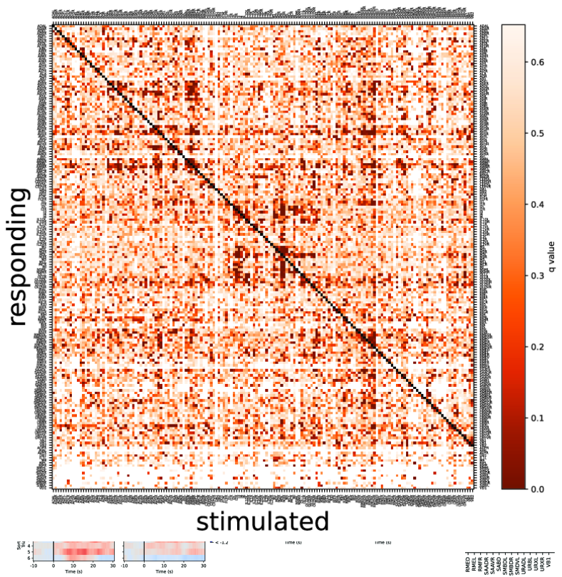
Extended Data Figure 4: Observations and false discovery rate of neuron pairs in the signal propagation map. a) Number of observations made of each neuron pair for WT-background animals. To be considered an observation, the upstream neuron must have been stimulated, calcium imaging of both the upstream and downstream neuron must have been recorded, and the upstream neuron must have exhibited an auto-response. Sorted as in Extended Data Figure 3a. Reverse cumulative distribution is also shown (bottom panel) and reports the fraction of pairs (number of observed pairs divided by the total number of possible pairs of neurons in the head). b) $q$-values are shown for each neuron pair. $q$-values report false discovery rate of finding a functional connection. They provide a metric of significance for assessing whether a neuron pair is functionally connected based on the number of observations and the magnitude of the response transients, taking into consideration the number of multiple hypothesis tested. Cumulative distribution is also shown (bottom panel). c) ASGR often exhibits activity immediately following stimulation of AVJR, but because its $q$-value is greater than 0.05, it does not meet the stringent statistical threshold to be deemed “functionally connected.”

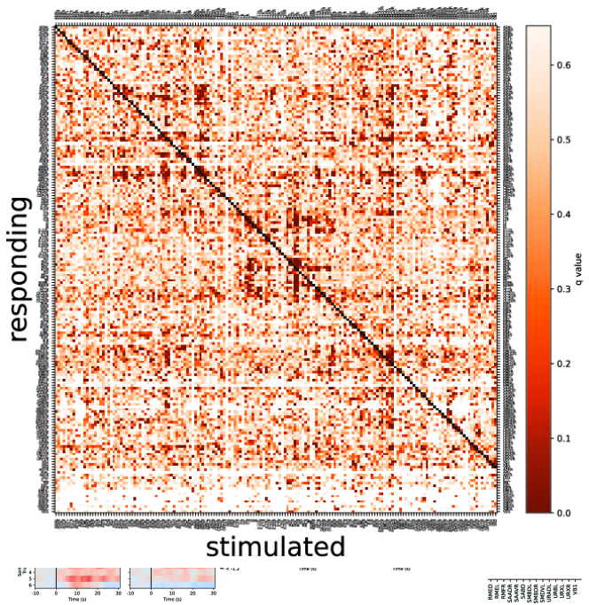
Extended Data Figure 5: Signal propagation map showing false discovery rates for functional connections and non-connections. a) Map of functional connections showing downstream calcium response amplitude and false discovery rate for WT. Same as Fig. 2 except here neurons that are observed but not stimulated are also included. Note the colorbar has two axes. Mean amplitude of neural activity in a post-stimulus time window ($\langle\Delta F/F_{0}\rangle_{t}$) averaged across trials and individuals is shown. $q$-value reports false discovery rate (more gray is less significant). White indicates no measurement. Auto-response is required for inclusion and not displayed (black diagonal). ($N$=113 animals). b) Map of functionally not connected pairs. The false discovery rate, $q_{\mathrm{eq}}$, is reported for declaring a neuron pair to be not functionally connected. Lower $q_{\mathrm{eq}}$ (more red) indicates higher confidence that the observed downstream calcium activity is equivalent within a bound $\epsilon$ to a null distribution of spontaneous activity. The false-discovery rate takes into consideration the amplitude of the calcium transient, the number of observations and the number of hypotheses tested.

Extended Data Figure 6: Timescales and variability of measured functional connectivity. WT. a) The fraction of stimulation events that evoked a downstream “response” is shown for each neuron pair. To be classified as a “response” requires a sufficiently large calcium transient amplitude and derivative. Auto-responses are required and not shown (black diagonal). b) Kernels are functions that return the downstream neuron’s activity when convolved with the upstream neuron’s activity. Kernels capture properties of the connection independent of variability in the upstream neuron’s auto-response. Kernels are shown for each c) FLP response to AQR stimulation. Kernels are only calculated for stimuli that evoked downstream “responses” (indicated in orange). d) Kernel rise time for each measured neuron pair in WT is a metric of signal propagation speed. e) The stereotypy of kernels within each neuron pair is reported by calculating the average correlation coefficient among them. Only neuron pairs with at least two kernels are considered. f) Distribution of the correlation-coefficients of convolved kernels, within each pair of neurons (blue, n=30,406), and across all kernels measured regardless of neuron pair (orange, n = 113,880,912).

Extended Data Figure 7: Signal propagation of unc-31 background, with defects in dense-core vesicle-mediated extrasynaptic signaling. a) Same format as Extended Data Figure 5a. Mean amplitude of neural activity in a post-stimulus time window ($\langle\Delta F/F_{0}\rangle_{t}$) averaged across trials and individuals is shown. $q$-value reports false discovery rate and is a metric of significance (more gray is less significant). White indicates no measurement. Auto-response is required and not displayed (black diagonal). ($N$=18 animals). b) unc-31 mutants had a smaller proportion of measured pairwise neurons that were functionally connected ($q<0.05$) than WT (comparison run on pairs for which data is present in both WT and unc-31 mutants). c) Responses to RID stimulation are shown for WT (blue) and unc-31 (orange). Points are responses, bar is mean across trials and animals. Neurons with the smallest amplitude responses are not shown. Corresponding traces for ADLR, AWBR and URXL are shown in Fig. 4. As in that figure, responses here are shown even for those cases when RID’s calcium activity was not measured and therefore do not appear in a. Different inclusion criteria are used here to accommodate cases where the tagRFP-T expression is dim, as described in methods.

Extended Data Figure 8: Neural responses for some pairs are similar in wild-type and unc-31 mutant animals. Paired stimulus and response traces of selected neuron pairs with a-c) monosynaptic gap junctions or d) monosynaptic chemical synapses are shown in WT background (left) and unc-31 mutant background (right).

Extended Data Figure 9: Examples of candidate purely extrasynaptic pairs. a)$\langle\Delta F/F\rangle$ vs number of observations for our candidate purely extrasynaptic-dependent pairs. Arrows indicate examples shown below. b)List of candidate entirely extrasynaptic-dependent connections. Relevant neuropeptide GPCR expression is listed in Supporting Spreadsheet 1, compiled from [97, 78], following [96]. c-e) Paired responses in WT and unc-31 animals for the candidate extrasynaptic pairs AVER->RMDDR, AVDR->ASHR, and RMDDR->RMDDL respectively, selected among all the candidates as illustrated in panel (a)

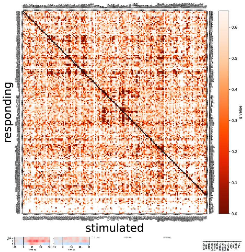
Extended Data Figure 10: Selected instances of agreement between measured signal propagation and previously reported functional measurements.

Supplementary Material

Supplementary Spreadsheet 1

https://doi.org/10.6084/m9.figshare.23057558 Microsoft Excel file lists neuropeptide and GPCR combinations for putative purely extrasynaptic-dependent signaling pairs of neurons. Neuropeptide and GPCR combinations are automatically generated based on data from [97, 78], following [96].]

Supplementary Movie 1

M1 stimulation evokes pharyngeal muscle contraction. Video from four animals are shown during signal propagation measurements. In each example, neuron M1 is optogenetically stimulated for 0.5 s and pharyngeal muscle contractions are visible by their effect on the location of neighboring neurons. M1 is known to release acetylcholine via chemical synapse onto pharyngeal muscles [63, 64]. Top panel shows z-projection of tagRFP-T. Bottom panel shows z-projection of GCaMP6 fluorescence. Crosshairs indicate neuron currently targeted for stimulation.

References

- [1] Mesulam, M. Imaging connectivity in the human cerebral cortex: The next frontier? \JournalTitleAnnals of Neurology 57, 5–7, DOI: 10.1002/ana.20368 (2005). _eprint: https://onlinelibrary.wiley.com/doi/pdf/10.1002/ana.20368.
- [2] Seung, H. S. Towards functional connectomics. \JournalTitleNature 471, 171–172, DOI: 10.1038/471170a (2011). Number: 7337 Publisher: Nature Publishing Group.
- [3] Abbott, L. F. et al. The Mind of a Mouse. \JournalTitleCell 182, 1372–1376, DOI: 10.1016/j.cell.2020.08.010 (2020).
- [4] Helmstaedter, M. et al. Connectomic reconstruction of the inner plexiform layer in the mouse retina. \JournalTitleNature 500, 168–174, DOI: 10.1038/nature12346 (2013).
- [5] Hildebrand, D. G. C. et al. Whole-brain serial-section electron microscopy in larval zebrafish. \JournalTitleNature 545, 345–349, DOI: 10.1038/nature22356 (2017). Number: 7654 Publisher: Nature Publishing Group.
- [6] Scheffer, L. K. et al. A connectome and analysis of the adult Drosophila central brain. \JournalTitleeLife 9, e57443, DOI: 10.7554/eLife.57443 (2020). Publisher: eLife Sciences Publications, Ltd.
- [7] Dorkenwald, S. et al. FlyWire: online community for whole-brain connectomics. \JournalTitleNature Methods 19, 119–128, DOI: 10.1038/s41592-021-01330-0 (2022). Number: 1 Publisher: Nature Publishing Group.
- [8] Schneider-Mizell, C. M. et al. Quantitative neuroanatomy for connectomics in Drosophila. \JournalTitleeLife 5, e12059, DOI: 10.7554/eLife.12059 (2016). Publisher: eLife Sciences Publications, Ltd.
- [9] Eichler, K. et al. The complete connectome of a learning and memory centre in an insect brain. \JournalTitleNature 548, 175–182, DOI: 10.1038/nature23455 (2017).
- [10] White, J. G., Southgate, E., Thomson, J. N. & Brenner, S. The Structure of the Ventral Nerve Cord of Caenorhabditis elegans. \JournalTitlePhilosophical Transactions of the Royal Society of London. B, Biological Sciences 275, 327 –348, DOI: 10.1098/rstb.1976.0086 (1976).
- [11] Cook, S. J. et al. Whole-animal connectomes of both Caenorhabditis elegans sexes. \JournalTitleNature 571, 63–71, DOI: 10.1038/s41586-019-1352-7 (2019).
- [12] Witvliet, D. et al. Connectomes across development reveal principles of brain maturation. \JournalTitleNature 596, 257–261, DOI: 10.1038/s41586-021-03778-8 (2021). Bandiera_abtest: a Cg_type: Nature Research Journals Number: 7871 Primary_atype: Research Publisher: Nature Publishing Group Subject_term: Development of the nervous system;Developmental biology;Neural circuits;Neuroscience Subject_term_id: development-of-the-nervous-system;developmental-biology;neural-circuit;neuroscience.
- [13] Ryan, K., Lu, Z. & Meinertzhagen, I. A. The CNS connectome of a tadpole larva of Ciona intestinalis (L.) highlights sidedness in the brain of a chordate sibling. \JournalTitleeLife 5, e16962, DOI: 10.7554/eLife.16962 (2016). Publisher: eLife Sciences Publications, Ltd.
- [14] Verasztó, C. et al. Whole-animal connectome and cell-type complement of the three-segmented Platynereis dumerilii larva, DOI: 10.1101/2020.08.21.260984 (2020). Pages: 2020.08.21.260984 Section: New Results.
- [15] Briggman, K. L., Helmstaedter, M. & Denk, W. Wiring specificity in the direction-selectivity circuit of the retina. \JournalTitleNature 471, 183–188, DOI: 10.1038/nature09818 (2011). Number: 7337 Publisher: Nature Publishing Group.
- [16] Bock, D. D. et al. Network anatomy and in vivo physiology of visual cortical neurons. \JournalTitleNature 471, 177–182, DOI: 10.1038/nature09802 (2011). Number: 7337 Publisher: Nature Publishing Group.
- [17] Hulse, B. K. et al. A connectome of the Drosophila central complex reveals network motifs suitable for flexible navigation and context-dependent action selection. \JournalTitleeLife 10, e66039, DOI: 10.7554/eLife.66039 (2021). Publisher: eLife Sciences Publications, Ltd.
- [18] Kim, S. S., Rouault, H., Druckmann, S. & Jayaraman, V. Ring attractor dynamics in the Drosophila central brain. \JournalTitleScience eaal4835, DOI: 10.1126/science.aal4835 (2017).
- [19] Chalfie, M. et al. The neural circuit for touch sensitivity in Caenorhabditis elegans. \JournalTitleThe Journal of Neuroscience: The Official Journal of the Society for Neuroscience 5, 956–64, DOI: 3981252 (1985).
- [20] Gray, J. M., Hill, J. J. & Bargmann, C. I. A circuit for navigation in Caenorhabditis elegans. \JournalTitleProceedings of the National Academy of Sciences of the United States of America 102, 3184–3191, DOI: 10.1073/pnas.0409009101 (2005). PMC546636 PMID: 15689400.
- [21] Perkins, L. A., Hedgecock, E. M., Thomson, J. N. & Culotti, J. G. Mutant sensory cilia in the nematode Caenorhabditis elegans. \JournalTitleDevelopmental Biology 117, 456–487, DOI: 10.1016/0012-1606(86)90314-3 (1986).
- [22] Kunert-Graf, J. M., Shlizerman, E., Walker, A. & Kutz, J. N. Multistability and Long-Timescale Transients Encoded by Network Structure in a Model of C. elegans Connectome Dynamics. \JournalTitleFrontiers in Computational Neuroscience 11 (2017).
- [23] Mi, L. et al. Connectome-constrained latent variable models of whole-brain neural activity (2022).
- [24] Yan, G. et al. Network control principles predict neuron function in the Caenorhabditis elegans connectome. \JournalTitleNature 550, 519–523, DOI: 10.1038/nature24056 (2017). Number: 7677 Publisher: Nature Publishing Group.
- [25] Vaaga, C. E., Borisovska, M. & Westbrook, G. L. Dual-transmitter neurons: Functional implications of co-release and co-transmission. \JournalTitleCurrent opinion in neurobiology 0, 25–32, DOI: 10.1016/j.conb.2014.04.010 (2014).
- [26] O’Malley, D. M., Sandell, J. H. & Masland, R. H. Co-release of acetylcholine and GABA by the starburst amacrine cells. \JournalTitleJournal of Neuroscience 12, 1394–1408, DOI: 10.1523/JNEUROSCI.12-04-01394.1992 (1992). Publisher: Society for Neuroscience Section: Articles.
- [27] Johnson, M. D. Synaptic glutamate release by postnatal rat serotonergic neurons in microculture. \JournalTitleNeuron 12, 433–442, DOI: 10.1016/0896-6273(94)90283-6 (1994).
- [28] Yoo, J. H. et al. Ventral tegmental area glutamate neurons co-release GABA and promote positive reinforcement. \JournalTitleNature Communications 7, 13697, DOI: 10.1038/ncomms13697 (2016). Number: 1 Publisher: Nature Publishing Group.
- [29] Fisher, Y. E., Lu, J., D?Alessandro, I. & Wilson, R. I. Sensorimotor experience remaps visual input to a heading-direction network. \JournalTitleNature 576, 121–125, DOI: 10.1038/s41586-019-1772-4 (2019). Number: 7785 Publisher: Nature Publishing Group.
- [30] Franconville, R., Beron, C. & Jayaraman, V. Building a functional connectome of the Drosophila central complex. \JournalTitleeLife 7, e37017, DOI: 10.7554/eLife.37017 (2018). Publisher: eLife Sciences Publications, Ltd.
- [31] Harris-Warrick, R. M. & Marder, E. Modulation of Neural Networks for Behavior. \JournalTitleAnnual Review of Neuroscience 14, 39–57, DOI: 10.1146/annurev.ne.14.030191.000351 (1991). _eprint: https://doi.org/10.1146/annurev.ne.14.030191.000351.
- [32] Marder, E. Neuromodulation of Neuronal Circuits: Back to the Future. \JournalTitleNeuron 76, 1–11, DOI: 10.1016/j.neuron.2012.09.010 (2012).
- [33] Bargmann, C. I. Beyond the connectome: how neuromodulators shape neural circuits. \JournalTitleBioEssays: News and Reviews in Molecular, Cellular and Developmental Biology 34, 458–465, DOI: 10.1002/bies.201100185 (2012).
- [34] Bentley, B. et al. The Multilayer Connectome of Caenorhabditis elegans. \JournalTitlePLOS Computational Biology 12, e1005283, DOI: 10.1371/journal.pcbi.1005283 (2016). Publisher: Public Library of Science.
- [35] Panzeri, S., Moroni, M., Safaai, H. & Harvey, C. D. The structures and functions of correlations in neural population codes. \JournalTitleNature Reviews Neuroscience 1–17, DOI: 10.1038/s41583-022-00606-4 (2022). Publisher: Nature Publishing Group.
- [36] Lehky, S. R. & Sejnowski, T. J. Network model of shape-from-shading: neural function arises from both receptive and projective fields. \JournalTitleNature 333, 452–454, DOI: 10.1038/333452a0 (1988). Number: 6172 Publisher: Nature Publishing Group.
- [37] Lepage, K. Q., Ching, S. & Kramer, M. A. Inferring evoked brain connectivity through adaptive perturbation. \JournalTitleJournal of Computational Neuroscience 34, 303–318, DOI: 10.1007/s10827-012-0422-8 (2013).
- [38] Petreanu, L., Huber, D., Sobczyk, A. & Svoboda, K. Channelrhodopsin-2?assisted circuit mapping of long-range callosal projections. \JournalTitleNature Neuroscience 10, 663–668, DOI: 10.1038/nn1891 (2007). Number: 5 Publisher: Nature Publishing Group.
- [39] Huber, D. et al. Sparse optical microstimulation in barrel cortex drives learned behaviour in freely moving mice. \JournalTitleNature 451, 61–64, DOI: 10.1038/nature06445 (2008). Number: 7174 Publisher: Nature Publishing Group.
- [40] Zhang, Y.-P. & Oertner, T. G. Optical induction of synaptic plasticity using a light-sensitive channel. \JournalTitleNature Methods 4, 139–141, DOI: 10.1038/nmeth988 (2007). Number: 2 Publisher: Nature Publishing Group.
- [41] Emiliani, V., Cohen, A. E., Deisseroth, K. & Haeusser, M. All-Optical Interrogation of Neural Circuits. \JournalTitleJournal of Neuroscience 35, 13917–13926, DOI: 10.1523/JNEUROSCI.2916-15.2015 (2015). WOS:000366051800013.
- [42] Wilson, N. R., Runyan, C. A., Wang, F. L. & Sur, M. Division and subtraction by distinct cortical inhibitory networks in vivo. \JournalTitleNature 488, 343–348, DOI: 10.1038/nature11347 (2012). Number: 7411 Publisher: Nature Publishing Group.
- [43] Rickgauer, J. P., Deisseroth, K. & Tank, D. W. Simultaneous cellular-resolution optical perturbation and imaging of place cell firing fields. \JournalTitleNature Neuroscience 17, 1816–1824, DOI: 10.1038/nn.3866 (2014). Tex.pmcid: PMC4459599.
- [44] Packer, A. M., Russell, L. E., Dalgleish, H. W. P. & Häusser, M. Simultaneous all-optical manipulation and recording of neural circuit activity with cellular resolution in vivo. \JournalTitleNature Methods 12, 140–146, DOI: 10.1038/nmeth.3217 (2015). Bandiera_abtest: a Cg_type: Nature Research Journals Number: 2 Primary_atype: Research Publisher: Nature Publishing Group Subject_term: Fluorescence imaging;Neuroscience;Optogenetics Subject_term_id: fluorescence-imaging;neuroscience;optogenetics.
- [45] McRaven, C. et al. High-throughput cellular-resolution synaptic connectivity mapping in vivo with concurrent two-photon optogenetics and volumetric Ca2+ imaging. \JournalTitlebioRxiv 2020.02.21.959650, DOI: 10.1101/2020.02.21.959650 (2020). Publisher: Cold Spring Harbor Laboratory Section: New Results.
- [46] Chen, C. et al. Functional architecture of neural circuits for leg proprioception in Drosophila. \JournalTitleCurrent Biology 31, 5163–5175.e7, DOI: 10.1016/j.cub.2021.09.035 (2021).
- [47] Guo, Z. V., Hart, A. C. & Ramanathan, S. Optical interrogation of neural circuits in Caenorhabditis elegans. \JournalTitleNature methods 6, 891–896, DOI: 10.1038/nmeth.1397 (2009).
- [48] Nguyen, J. P. et al. Whole-brain calcium imaging with cellular resolution in freely behaving Caenorhabditis elegans. \JournalTitleProceedings of the National Academy of Sciences 113, E1074–E1081, DOI: 10.1073/pnas.1507110112 (2016).
- [49] Venkatachalam, V. et al. Pan-neuronal imaging in roaming Caenorhabditis elegans. \JournalTitleProceedings of the National Academy of Sciences of the United States of America 113, E1082–1088, DOI: 10.1073/pnas.1507109113 (2016).
- [50] Denk, W., Strickler, J. H. & Webb, W. W. Two-photon laser scanning fluorescence microscopy. \JournalTitleScience (New York, N.Y.) 248, 73–76 (1990).
- [51] Rickgauer, J. P. & Tank, D. W. Two-photon excitation of channelrhodopsin-2 at saturation. \JournalTitleProceedings of the National Academy of Sciences 106, 15025–15030, DOI: 10.1073/pnas.0907084106 (2009). Publisher: Proceedings of the National Academy of Sciences.
- [52] Andrasfalvy, B. K., Zemelman, B. V., Tang, J. & Vaziri, A. Two-photon single-cell optogenetic control of neuronal activity by sculpted light. \JournalTitleProceedings of the National Academy of Sciences 107, 11981–11986, DOI: 10.1073/pnas.1006620107 (2010). Publisher: Proceedings of the National Academy of Sciences.
- [53] Yang, W., Carrillo-Reid, L., Bando, Y., Peterka, D. S. & Yuste, R. Simultaneous two-photon imaging and two-photon optogenetics of cortical circuits in three dimensions. \JournalTitleeLife 7, DOI: 10.7554/eLife.32671 (2018).
- [54] Zhang, Z., Russell, L. E., Packer, A. M., Gauld, O. M. & Häusser, M. Closed-loop all-optical interrogation of neural circuits in vivo. \JournalTitleNature Methods 15, 1037, DOI: 10.1038/s41592-018-0183-z (2018).
- [55] Russell, L. E. et al. All-optical interrogation of neural circuits in behaving mice. \JournalTitleNature Protocols 1–42, DOI: 10.1038/s41596-022-00691-w (2022). Publisher: Nature Publishing Group.
- [56] Bhatla, N. & Horvitz, H. R. Light and hydrogen peroxide inhibit C. elegans Feeding through gustatory receptor orthologs and pharyngeal neurons. \JournalTitleNeuron 85, 804–818, DOI: 10.1016/j.neuron.2014.12.061 (2015).
- [57] Quintin, S., Aspert, T., Ye, T. & Charvin, G. Distinct mechanisms underlie H2O2 sensing in C. elegans head and tail. \JournalTitlePLOS ONE 17, e0274226, DOI: 10.1371/journal.pone.0274226 (2022). Publisher: Public Library of Science.
- [58] Chen, T.-W. et al. Ultrasensitive fluorescent proteins for imaging neuronal activity. \JournalTitleNature 499, 295–300, DOI: 10.1038/nature12354 (2013). Tex.copyright: © 2013 Nature Publishing Group, a division of Macmillan Publishers Limited. All Rights Reserved.
- [59] Bhatla, N., Droste, R., Sando, S. R., Huang, A. & Horvitz, H. R. Distinct Neural Circuits Control Rhythm Inhibition and Spitting by the Myogenic Pharynx of C. elegans. \JournalTitleCurrent biology: CB 25, 2075–2089, DOI: 10.1016/j.cub.2015.06.052 (2015).
- [60] Gordus, A., Pokala, N., Levy, S., Flavell, S. W. & Bargmann, C. I. Feedback from network states generates variability in a probabilistic olfactory circuit. \JournalTitleCell 161, 215–227, DOI: 10.1016/j.cell.2015.02.018 (2015).
- [61] Li, Z., Liu, J., Zheng, M. & Xu, X. Z. S. Encoding of Both Analog- and Digital-like Behavioral Outputs by One C. elegans Interneuron. \JournalTitleCell 159, 751–765, DOI: 10.1016/j.cell.2014.09.056 (2014).
- [62] Lin, A. et al. Functional imaging and quantification of multineuronal olfactory responses in C. elegans. \JournalTitleScience Advances 9, eade1249, DOI: 10.1126/sciadv.ade1249 (2023). Publisher: American Association for the Advancement of Science.
- [63] Franks, C. J., Murray, C., Ogden, D., O’Connor, V. & Holden-Dye, L. A comparison of electrically evoked and channel rhodopsin-evoked postsynaptic potentials in the pharyngeal system of Caenorhabditis elegans. \JournalTitleInvertebrate neuroscience: IN 9, 43–56, DOI: 10.1007/s10158-009-0088-8 (2009).
- [64] Sando, S. R., Bhatla, N., Lee, E. L. & Horvitz, H. R. An hourglass circuit motif transforms a motor program via subcellularly localized muscle calcium signaling and contraction. \JournalTitleeLife 10, e59341, DOI: 10.7554/eLife.59341 (2021). Publisher: eLife Sciences Publications, Ltd.
- [65] Bhatla, N. C. elegans - Interactive Neural Network (2009).
- [66] Yemini, E. et al. NeuroPAL: A Multicolor Atlas for Whole-Brain Neuronal Identification in C. elegans. \JournalTitleCell 184, 272–288.e11, DOI: 10.1016/j.cell.2020.12.012 (2021).
- [67] Hardaker, L. A., Singer, E., Kerr, R., Zhou, G. & Schafer, W. R. Serotonin modulates locomotory behavior and coordinates egg-laying and movement in Caenorhabditis elegans. \JournalTitleJournal of Neurobiology 49, 303–313, DOI: 10.1002/neu.10014 (2001). _eprint: https://onlinelibrary.wiley.com/doi/pdf/10.1002/neu.10014.
- [68] Wicks, S. R., Roehrig, C. J. & Rankin, C. H. A dynamic network simulation of the nematode tap withdrawal circuit: predictions concerning synaptic function using behavioral criteria. \JournalTitleThe Journal of Neuroscience: The Official Journal of the Society for Neuroscience 16, 4017–4031 (1996).
- [69] Kawano, T. et al. An Imbalancing Act: Gap Junctions Reduce the Backward Motor Circuit Activity to Bias C. elegans for Forward Locomotion. \JournalTitleNeuron 72, 572–586, DOI: 10.1016/j.neuron.2011.09.005 (2011).
- [70] White, J. G., Southgate, E., Thomson, J. N. & Brenner, S. The Structure of the Nervous System of the Nematode Caenorhabditis elegans. \JournalTitlePhilosophical Transactions of the Royal Society of London. Series B, Biological Sciences 314, 1–340 (1986).
- [71] Chronis, N., Zimmer, M. & Bargmann, C. I. Microfluidics for in vivo imaging of neuronal and behavioral activity in Caenorhabditis elegans. \JournalTitleNature Methods 4, 727–731, DOI: 10.1038/nmeth1075 (2007).
- [72] Arous, J. B., Tanizawa, Y., Rabinowitch, I., Chatenay, D. & Schafer, W. R. Automated imaging of neuronal activity in freely behaving Caenorhabditis elegans. \JournalTitleJournal of Neuroscience Methods DOI: 10.1016/j.jneumeth.2010.01.011 (2010).
- [73] Shipley, F. B., Clark, C. M., Alkema, M. J. & Leifer, A. M. Simultaneous optogenetic manipulation and calcium imaging in freely moving C. elegans. \JournalTitleFrontiers in Neural Circuits 8, DOI: 10.3389/fncir.2014.00028 (2014).
- [74] Kato, S. et al. Global brain dynamics embed the motor command sequence of Caenorhabditis elegans. \JournalTitleCell 163, 656–669, DOI: 10.1016/j.cell.2015.09.034 (2015).
- [75] Wang, Y. et al. Flexible motor sequence generation during stereotyped escape responses. \JournalTitleeLife 9, e56942, DOI: 10.7554/eLife.56942 (2020). Publisher: eLife Sciences Publications, Ltd.
- [76] Faumont, S. et al. An Image-Free Opto-Mechanical System for Creating Virtual Environments and Imaging Neuronal Activity in Freely Moving Caenorhabditis elegans. \JournalTitlePLoS ONE 6, e24666, DOI: 10.1371/journal.pone.0024666 (2011).
- [77] Fenyves, B. G., Szilágyi, G. S., Vassy, Z., S?ti, C. & Csermely, P. Synaptic polarity and sign-balance prediction using gene expression data in the Caenorhabditis elegans chemical synapse neuronal connectome network. \JournalTitlePLOS Computational Biology 16, e1007974, DOI: 10.1371/journal.pcbi.1007974 (2020). Publisher: Public Library of Science.
- [78] Taylor, S. R. et al. Molecular topography of an entire nervous system. \JournalTitleCell 184, 4329–4347.e23, DOI: 10.1016/j.cell.2021.06.023 (2021).
- [79] Jones, A. K. & Sattelle, D. B. The cys-loop ligand-gated ion channel gene superfamily of the nematode, Caenorhabditis elegans. \JournalTitleInvertebrate Neuroscience 8, 41–47, DOI: 10.1007/s10158-008-0068-4 (2008).
- [80] Benjamini, Y. & Hochberg, Y. Controlling the False Discovery Rate: A Practical and Powerful Approach to Multiple Testing. \JournalTitleJournal of the Royal Statistical Society. Series B (Methodological) 57, 289–300 (1995). Publisher: [Royal Statistical Society, Wiley].
- [81] Storey, J. D. & Tibshirani, R. Statistical significance for genomewide studies. \JournalTitleProceedings of the National Academy of Sciences 100, 9440–9445, DOI: 10.1073/pnas.1530509100 (2003). Publisher: Proceedings of the National Academy of Sciences.
- [82] Uzel, K., Kato, S. & Zimmer, M. A set of hub neurons and non-local connectivity features support global brain dynamics in C. elegans. \JournalTitleCurrent Biology DOI: 10.1016/j.cub.2022.06.039 (2022).
- [83] van Vreeswijk, C. & Sompolinsky, H. Chaos in Neuronal Networks with Balanced Excitatory and Inhibitory Activity. \JournalTitleScience 274, 1724–1726 (1996). Publisher: American Association for the Advancement of Science.
- [84] Isaacson, J. S. & Scanziani, M. How Inhibition Shapes Cortical Activity. \JournalTitleNeuron 72, 231–243, DOI: 10.1016/j.neuron.2011.09.027 (2011).
- [85] Meinecke, D. L. & Peters, A. GABA immunoreactive neurons in rat visual cortex. \JournalTitleJournal of Comparative Neurology 261, 388–404, DOI: 10.1002/cne.902610305 (1987). _eprint: https://onlinelibrary.wiley.com/doi/pdf/10.1002/cne.902610305.
- [86] Stern, S., Kirst, C. & Bargmann, C. I. Neuromodulatory Control of Long-Term Behavioral Patterns and Individuality across Development. \JournalTitleCell 171, 1649–1662.e10, DOI: 10.1016/j.cell.2017.10.041 (2017).
- [87] Varshney, L. R., Chen, B. L., Paniagua, E., Hall, D. H. & Chklovskii, D. B. Structural Properties of the Caenorhabditis elegans Neuronal Network. \JournalTitlePLoS Comput Biol 7, e1001066, DOI: 10.1371/journal.pcbi.1001066 (2011).
- [88] Kunert, J., Shlizerman, E. & Kutz, J. N. Low-dimensional functionality of complex network dynamics: Neurosensory integration in the Caenorhabditis connectome. \JournalTitlePhysical Review E 89, 052805, DOI: 10.1103/PhysRevE.89.052805 (2014).
- [89] Narayan, A., Laurent, G. & Sternberg, P. W. Transfer characteristics of a thermosensory synapse in Caenorhabditis elegans. \JournalTitleProceedings of the National Academy of Sciences of the United States of America 108, 9667–9672, DOI: 10.1073/pnas.1106617108 (2011).
- [90] Kuramochi, M. & Doi, M. An Excitatory/Inhibitory Switch From Asymmetric Sensory Neurons Defines Postsynaptic Tuning for a Rapid Response to NaCl in Caenorhabditis elegans. \JournalTitleFrontiers in Molecular Neuroscience 11 (2019).
- [91] Agnati, L. F., Zoli, M., Strömberg, I. & Fuxe, K. Intercellular communication in the brain: wiring versus volume transmission. \JournalTitleNeuroscience 69, 711–726, DOI: 10.1016/0306-4522(95)00308-6 (1995).
- [92] Brickley, S. G. & Mody, I. Extrasynaptic GABAA Receptors: Their Function in the CNS and Implications for Disease. \JournalTitleNeuron 73, 23–34, DOI: 10.1016/j.neuron.2011.12.012 (2012).
- [93] Shen, Y. et al. An extrasynaptic GABAergic signal modulates a pattern of forward movement in Caenorhabditis elegans. \JournalTitleeLife 5, e14197, DOI: 10.7554/eLife.14197 (2016). Publisher: eLife Sciences Publications, Ltd.
- [94] Hardingham, G. E. & Bading, H. Synaptic versus extrasynaptic NMDA receptor signalling: implications for neurodegenerative disorders. \JournalTitleNature Reviews Neuroscience 11, 682–696, DOI: 10.1038/nrn2911 (2010). Number: 10 Publisher: Nature Publishing Group.
- [95] Taghert, P. H. & Nitabach, M. N. Peptide neuromodulation in invertebrate model systems. \JournalTitleNeuron 76, 82–97, DOI: 10.1016/j.neuron.2012.08.035 (2012).
- [96] Ripoll-Sánchez, L. et al. The neuropeptidergic connectome of C. elegans, DOI: 10.1101/2022.10.30.514396 (2022). Pages: 2022.10.30.514396 Section: New Results.
- [97] Beets, I. et al. System-wide mapping of neuropeptide-GPCR interactions in C. elegans, DOI: 10.1101/2022.10.30.514428 (2022). Pages: 2022.10.30.514428 Section: New Results.
- [98] Smith, S. J. et al. Single-cell transcriptomic evidence for dense intracortical neuropeptide networks. \JournalTitleeLife 8, e47889, DOI: 10.7554/eLife.47889 (2019). Publisher: eLife Sciences Publications, Ltd.
- [99] Pelletier, G., Leclerc, R. & Dupont, A. Electron microscope immunohistochemical localization of substance P in the central nervous system of the rat. \JournalTitleJournal of Histochemistry & Cytochemistry 25, 1373–1375, DOI: 10.1177/25.12.925343 (1977). Publisher: Journal of Histochemistry & Cytochemistry.
- [100] Speese, S. et al. UNC-31 (CAPS) Is Required for Dense-Core Vesicle But Not Synaptic Vesicle Exocytosis in Caenorhabditis elegans. \JournalTitleThe Journal of Neuroscience 27, 6150–6162, DOI: 10.1523/JNEUROSCI.1466-07.2007 (2007).
- [101] Golowasch, J. & Marder, E. Proctolin activates an inward current whose voltage dependence is modified by extracellular Ca2+. \JournalTitleJournal of Neuroscience 12, 810–817, DOI: 10.1523/JNEUROSCI.12-03-00810.1992 (1992). Publisher: Society for Neuroscience Section: Articles.
- [102] Lim, M. A. et al. Neuroendocrine modulation sustains the C. elegans forward motor state. \JournalTitleeLife 5, e19887, DOI: 10.7554/eLife.19887 (2016).
- [103] Hendricks, M., Ha, H., Maffey, N. & Zhang, Y. Compartmentalized calcium dynamics in a C. elegans interneuron encode head movement. \JournalTitleNature 487, 99–103, DOI: 10.1038/nature11081 (2012).
- [104] Randi, F. & Leifer, A. M. Nonequilibrium Green’s Functions for Functional Connectivity in the Brain. \JournalTitlePhysical Review Letters 126, 118102, DOI: 10.1103/PhysRevLett.126.118102 (2021).
- [105] Lin, A. et al. Functional imaging and quantification of multi-neuronal olfactory responses in C. elegans, DOI: 10.1101/2022.05.27.493772 (2022). Pages: 2022.05.27.493772 Section: New Results.
- [106] Lindsay, T. H., Thiele, T. R. & Lockery, S. R. Optogenetic analysis of synaptic transmission in the central nervous system of the nematode Caenorhabditis elegans. \JournalTitleNature Communications 2, 306, DOI: 10.1038/ncomms1304 (2011).
- [107] Noma, K. & Jin, Y. Rapid Integration of Multi-copy Transgenes Using Optogenetic Mutagenesis in Caenorhabditis elegans. \JournalTitleG3 Genes Genomes Genetics 8, 2091–2097, DOI: 10.1534/g3.118.200158 (2018).
- [108] Evans, T. Transformation and microinjection. In WormBook (2006). Doi/10.1895/wormbook.1.108.1.
- [109] Yu, X. et al. Fast deep learning correspondence for neuron tracking and identification in C.elegans using synthetic training. DOI: 10.17605/OSF.IO/T7DZU (2021).
- [110] Paix, A., Folkmann, A. & Seydoux, G. Precision genome editing using CRISPR-Cas9 and linear repair templates in C. elegans. \JournalTitleMethods (San Diego, Calif.) 121-122, 86–93, DOI: 10.1016/j.ymeth.2017.03.023 (2017).
- [111] Monsalve, G. C., Yamamoto, K. R. & Ward, J. D. A New Tool for Inducible Gene Expression in Caenorhabditis elegans. \JournalTitleGenetics 211, 419–430, DOI: 10.1534/genetics.118.301705 (2019).
- [112] Nguyen, J. P. et al. Whole-brain calcium imaging with cellular resolution in freely behaving Caenorhabditis elegans. \JournalTitleProceedings of the National Academy of Sciences 201507110, DOI: 10.1073/pnas.1507110112 (2015).
- [113] Hallinen, K. M. et al. Decoding locomotion from population neural activity in moving C. elegans. \JournalTitleeLife 10, e66135, DOI: 10.7554/eLife.66135 (2021). Publisher: eLife Sciences Publications, Ltd.
- [114] Nguyen, J. P., Linder, A. N., Plummer, G. S., Shaevitz, J. W. & Leifer, A. M. Automatically tracking neurons in a moving and deforming brain. \JournalTitlePLOS Computational Biology 13, e1005517, DOI: 10.1371/journal.pcbi.1005517 (2017).
- [115] Zhou, Z. et al. Accurate and Robust Non-rigid Point Set Registration using Student?s-t Mixture Model with Prior Probability Modeling. \JournalTitleScientific Reports 8, 8742, DOI: 10.1038/s41598-018-26288-6 (2018). Number: 1 Publisher: Nature Publishing Group.
- [116] Papagiakoumou, E., Sars, V. d., Oron, D. & Emiliani, V. Patterned two-photon illumination by spatiotemporal shaping of ultrashort pulses. \JournalTitleOptics Express 16, 22039–22047, DOI: 10.1364/OE.16.022039 (2008). Publisher: Optica Publishing Group.
- [117] Schuirmann, D. J. A comparison of the Two One-Sided Tests Procedure and the Power Approach for assessing the equivalence of average bioavailability. \JournalTitleJournal of Pharmacokinetics and Biopharmaceutics 15, 657–680, DOI: 10.1007/BF01068419 (1987).
- [118] Izquierdo, E. J. & Beer, R. D. From head to tail: a neuromechanical model of forward locomotion in Caenorhabditis elegans. \JournalTitlePhilosophical Transactions of the Royal Society of London. Series B, Biological Sciences 373, 20170374, DOI: 10.1098/rstb.2017.0374 (2018).
- [119] Frooninckx, L. et al. Neuropeptide GPCRs in C. elegans. \JournalTitleFrontiers in Endocrinology 3 (2012).
Acknowledgments
We thank Annegret Falkner, Mala Murthy, Eva Naumann, H. Sebastian Seung, Jacob Bien and Josh Shaevitz for comments on the manuscript. Online visualization software was created by Research Computing staff in the Lewis-Sigler Institute for Integrative Genomics and the Princeton Neuroscience Institute with special thanks to Fan Kang, Robert Leach, Ben Singer, and Lance Parsons.