New bounds for the number of connected components of fewnomial hypersurfaces

Abstract

We prove that the zero set of a $5$-nomial in $n$ variables, whose exponent vectors are not colinear, has at most $\lfloor\frac{n-1}{2}\rfloor+3$ connected components in the positive orthant. Moreover, we give an explicit $5$-nomial in $2$ variables which defines a curve with three connected components in the posititive orthant, showing that our bound is sharp for $n=2$. In a more general setting, if $\operatorname{\mathcal{A}}=\{a_{0},\ldots,a_{d+k}\}\subset\operatorname{\mathbb{Z}}^{n}$ has dimension $d$, we prove that the number of connected components of the zero set of a $\operatorname{\mathcal{A}}$-polynomial in the positive orthant is smaller than or equal to $18(d+1)^{k-1}2^{\binom{k-1}{2}}+k+1$, improving the previously known bounds. Moreover, our results continue to work for polynomials with real exponents.

1 Introduction

Descartes’ rule of signs implies that the number of positive solutions of a univariate polynomial is bounded by a function which only depends on its number of monomials. The Fewnomials Theory, developped by Khovanskiĭ [19] generalizes this result for multivariate polynomials and more general functions.

In its monograph, Khovanskiĭ considered smooth hypersurfaces in the positive orthant $\operatorname{\mathbb{R}}_{>0}^{n}$ defined by polynomials with $n+k+1$ monomials. He showed [[19], Sec. 3.14, Cor. 4] that the total Betti number (and so the number of connected components) of such a fewnomial hypersurface is at most

$$(2n^{2}-n+1)^{n+k}(2n)^{n-1}2^{\binom{n+k}{2}}.$$

The breakthrough was that the bound is only depending on $n$ and on the number of monomials (and so holds true whatever is the degree of the considered polynomial). Even if this upper bound was expected to be far from optimal, only few quantitative improvements have been found. The upper bound on the number of connected components was first improved by Li, Rojas, and Wang [20], Perrucci [22], and Bihan, Rojas, and Sottile [6]. In the latter paper the authors showed that a smooth hypersurface in $(\operatorname{\mathbb{R}}_{>0})^{n}$ defined by a polynomial with $d+k+1$ monomials whose exponent vectors have $d$-dimensional affine span has fewer than

$$\frac{e+3}{4}2^{\binom{k+1}{2}}2^{d}d^{k+1}$$

connected components. The approach was based on Bihan and Sottile’s improved bound on the number of positive solutions of a system supported on few monomials [8].

In a subsequent work, Bihan and Sottile [10] improved again their bound. They show that the sum of Betti numbers of such an hypersurface was bounded by

$$\frac{e^{2}+3}{4}2^{\binom{k}{2}}\sum_{i=0}^{d}\binom{d}{i}i^{k}$$

which already gives the better bound

$$(e^{2}+3)2^{\binom{k}{2}}d^{k}2^{d-3}.$$

The approach was based on the stratified Morse theory which was developped in [16].

More recently, the authors in [14] give a new bound which is in particular not anymore exponential in $d$. Taking our notations, they showed that if $f$ is a $n$-variate polynomial of support of cardinal $(d+k+1)$ and not lying in an affine hyperplane, then, for generic coeffients, the positive zero set of $f$ has no more than

$$\binom{d+k+1}{2}+2^{\binom{k-1}{2}}(d+2)^{k-1}$$

connected components. Furthermore, for $k=2$, a sharper upper bound of $\frac{(d+3)(d+2)}{2}+\lfloor\frac{d+5}{2}\rfloor$ is given.

However, it seems that there is a problem in their proof since they claim (Proposition 3.4 in [14]) that the number of non-simplicial faces of a $d$-dimensional polytope with $d+k+1$ vertices is at most $k$. In particular, a cube is a $3$-dimensional polytope (giving $k=4$) with already $6$ faces (the $2$-dimensional faces) which are non-simplicial. The situation happens to be even more problematic, since it can be shown (see Proposition 7.1) that the number of non-defective faces can be exponential in $k$.

Our results

In this paper, we improve the upper bounds on the number of connected components of the positive part of an hypersurface. We will mainly follow the “$\operatorname{\mathcal{A}}$-philosophy” developped by Gel’fand, Kapranov, and Zelevinsky [15]. In the following, let $\operatorname{\mathcal{A}}$ be a finite set in $\operatorname{\mathbb{R}}^{n}$ which spans an affine space of dimension $d$. The cardinal of $\operatorname{\mathcal{A}}$ is written as $d+k+1$. The parameter $k$ is called the codimension of $\operatorname{\mathcal{A}}$.

We give here our main results (see the theorems below to get stronger versions with more precise hypotheses).

Our new bound on the number of positive connected components in the general case is again polynomial in $d$ when $k$ is fixed.

Theorem (Theorem 7.4).

Let $\operatorname{\mathcal{A}}$ be a finite set in $\operatorname{\mathbb{R}}^{n}$ of dimension $d$ such that $\operatorname{codim}\operatorname{\mathcal{A}}=k$. For any real polynomial $f=\sum_{a\in\operatorname{\mathcal{A}}}c_{a}x^{a}$, we have

$$b_{0}(V_{>0}(f))\leq\frac{e^{2}+3}{4}\sum_{\kappa=1}^{k}\binom{d+k+1}{k-\kappa}2^{\binom{\kappa-1}{2}}(d+1)^{\kappa-1}.$$

The bound can be replaced by the weaker but simpler expression

$$b_{0}(V_{>0}(f))\leq 18(d+1)^{k-1}2^{\binom{k-1}{2}}+k+1.$$

The approach of the proof is close to that of [14]. However, we improve the bound obtained for the extremal $t$ case (see Theorem 6.2) and we correct the bound on the number of non-simplicial faces of a polytope.

Then, we focus on the case of codimension $2$. In this case, a finer analysis of the Gale dual of a critical system as well as the bounds obtained in [3] for the number of positive solutions of a system supported by a circuit enable us to prove the following result.

Theorem (Theorems 7.6 and 7.7).

If $\operatorname{\mathcal{A}}$ is a finite set of $\operatorname{\mathbb{R}}^{n}$ of dimension $d$ and codimension $2$, then $b_{0}(V_{>0}(f))\leq\left\lfloor\frac{d-1}{2}\right\rfloor+3$.

This bound is optimal for $d=2$, indeed we show that the bivariate polynomial $f(x,y)=1+x^{4}-xy^{2}-x^{3}y^{2}+0.76x^{2}y^{3}$ has three connected components in its positive zero set (see Theorem 7.8).

To achieve these bounds, we will start by obtaining an upper bound for hypersurfaces constructed by Viro’s combinatorial patchworking, also called $T$-hypersurfaces (see for example [18]). They are defined by polynomials of the form $f_{t}(x)=\sum_{a\in\operatorname{\mathcal{A}}}c_{a}t^{h_{a}}x^{a}$ where $t$ is a small positive parameter. These polynomials are often called Viro polynomials. We think this intermediate result could be interesting for itself.

Theorem (Theorem 6.2).

Assume that $h\in\operatorname{\mathbb{R}}^{\operatorname{\mathcal{A}}}$ is generic. There exist $0<t_{1}$ such that for every $t\in\left]0,t_{1}\right]$, $f_{t}=0$ has at most $k+1$ connected components in $(\operatorname{\mathbb{R}}_{>0})^{n}$.

If $n\geq 2$ and $k\geq 2$, then the bound can even be improved to $k$.

The ultimate goal is to estimate the number of connected components of $f_{t}(x)=0$ in $(\operatorname{\mathbb{R}}_{>0})^{n}$ when $t=1$. We analyze the set of $t\in]0,+\infty[$ for which the hypersurface $f_{t}(x)=0$ admits a singularity in the positive orthant or at infinity. This leads us to consider critical systems. When the function $h$ is sufficiently generic, these singularities are ordinary double points by a result of Forsgård [13] and the number of connected components varies at most by one. We detail this a bit more now using the easy examples of codimension $0$ and $1$.

Warm-up: the codimension $0$ and $1$ cases

We describe the general strategy and illustrate it in the easy (and well-known) cases of codimension $0$ and $1$. We decided to keep the objects intuitive in this warm-up to help the reader to understand the idea of the proof. The tools we use will be defined more formally in the next sections.

Let $\operatorname{\mathcal{A}}=\{a_{0},\ldots,a_{d+k}\}\subset\operatorname{\mathbb{R}}^{n}$ of dimension $d$. Let $f$ be a polynomial whose monomials have exponents $\operatorname{\mathcal{A}}$. The case $k=0$ arises when $\operatorname{\mathcal{A}}$ is the set of vertices of a simplex and an appropriate monomial change of variables transforms the positive zero set of $f$ into an affine hyperplane. Such a monomial change of coordinates gives rise to a diffeormorphism from the positive orthant to itself. In particular, the hypersurface defined by $f$ is never singular, and its positive part is either empty (when all coefficients of $f$ have the same sign) or diffeomorphic to the positive part of an affine hyperplane. A finite set $\operatorname{\mathcal{A}}\subset\operatorname{\mathbb{R}}^{n}$ for which there exists $a\in\operatorname{\mathcal{A}}$ such that $\operatorname{\mathcal{A}}\setminus\{a\}$ is contained in some affine subspace of dimension stricly smaller than $d=\dim\operatorname{\mathcal{A}}$ is called a pyramid. Note that if $\operatorname{\mathcal{A}}$ has codimension $0$ then it is a pyramid. Pyramidal sets provide another important family of sets $\operatorname{\mathcal{A}}$ with the property that the zero set of any polynomial $f=\sum_{a\in\operatorname{\mathcal{A}}}c_{a}x^{a}$ is non singular. This follows from the fact that if $\operatorname{\mathcal{A}}$ is pyramidal then via a monomial change of coordinates $f$ can tranformed into a polynomial of the form $x_{n}+g(x_{1},\ldots,x_{n-1})$. The case $k=1$ has been treated in [2] and [7] following the general strategy used in this paper.

Proposition 1.1.

Let $\operatorname{\mathcal{A}}=\{a_{0},\ldots,a_{d+k}\}\subset\operatorname{\mathbb{R}}^{n}$ of dimension $d$. Let $f$ be a polynomial in $\operatorname{\mathbb{R}}^{\operatorname{\mathcal{A}}}$ with non singular positive zero set $V_{>0}(f)=\{x\in(\operatorname{\mathbb{R}}_{>0})^{n}\mid f(x)=0\}$.

• If $k=0$, then $V_{>0}(f)$ is either empty or connected and non-compact.

• If $k=1$, then $V_{>0}(f)$ has at most $2$ connected components.

Write $f(x)=\sum_{a\in\operatorname{\mathcal{A}}}c_{a}x^{a}$. Let $h:\operatorname{\mathcal{A}}\rightarrow\operatorname{\mathbb{R}}$ be a generic function and consider the associated Viro polynomial $f_{t}(x)=\sum_{a\in\operatorname{\mathcal{A}}}c_{a}t^{h_{a}}x^{a}$. Assume that the positive zero set $V_{>0}(f)$ is non singular.

From Viro’s patchworking Theorem [29, 30], the topology of $V_{>0}(f_{t})$ is well understood when $t$ is small or large enough. We want to understand the topology of $V_{>0}(f_{t})$ when $t=1$. To do that it is sufficient to get $t$ moving and focus when the topology changes. Using stratified Morse theory (see the monograph [16]), it can happen only when a singularity appears. Let us be a bit more precise. A singularity can appear either inside the positive orthant, which corresponds to a positive solution of the critical system $f_{t}=x_{1}\partial f_{t}/\partial x_{1}=\cdots=x_{n}\partial f_{t}/\partial x_{n}=0$, or ”at infinity” which means that there exists a face $F$ of the convex hull $Q$ of $\operatorname{\mathcal{A}}$ such that the critical system associated to the truncated $f_{t}^{F}=\sum_{a\in\operatorname{\mathcal{A}}\cap F}c_{a}t^{h(a)}x^{a}$ has a positive solution. To highlight this fact, let us see it on an example which was given by Forsgård, Nisse, and Rojas (Example 3.7 in [14]). Taking $\operatorname{\mathcal{A}}=\{(0,0),(0,1),(0,2),(1,0),(1,2)\}$, the circle defined by $f_{0}=(x+1/2)^{2}+(y-2)^{2}-1=0$ intersects the positive orthant whereas the curve $f_{1}=(x+3/2)^{2}+(y-3/2)^{2}-1=0$ does not intersect the positive orthant (see Figure 1). However, the parameterized polynomial $f_{t}=(x+1/2+t)^{2}+(y-(4-t)/2)^{2}-1$ connects $f_{0}$ to $f_{1}$ and the hypersurface defined by $f_{t}$ has no singular point in the positive orthant for $t\in[0,1]$. In fact the change of topology comes from a singularity which appears in the $y$-axis. Indeed, if we consider the face $F$ of $Q$ given by the convex hull of $\{(0,0),(0,1),(0,2)\}$, we can notice that the hypersurface defined by the corresponding truncated polynomial $f_{t}^{F}=y^{2}+(t-4)y+5t^{2}/4-t+13/4$ has a singular point in the positive orthant for $t=1/2$.

Figure 1: The red circle defined by $f_{0}=0$ intersects the positive orthant and not the green one defined by $f_{1}=0$. The blue circle is the zero set of $f_{1/2}$.

Let us go back for a moment to the codimension $0$ case. Here, all intersections of $\operatorname{\mathcal{A}}$ with faces of $Q$ have codimension $0$. In particular, the hypersurfaces defined by $f_{t}$ and all its truncated do not have singular points in the corresponding positive orthants. Then the positive zero sets of polynomials $f_{t}$ are all homeomorphic. Consequently $V_{>0}(f)$ is either empty of connected and non-compact.

Let us consider now the codimension $1$ case. Thus, the configuration $\operatorname{\mathcal{A}}$ admits a unique affine relation, i.e., there exists a unique (up to multiplication by a scalar) vector $b=(b_{a})\in\operatorname{\mathbb{R}}^{\operatorname{\mathcal{A}}}$ such that $\sum_{a\in\operatorname{\mathcal{A}}}b_{a}=0$ and $\sum_{a\in\operatorname{\mathcal{A}}}b_{a}\cdot a=0$. Let $\operatorname{\mathcal{A}}^{\prime}$ be the support of $b$ (defined by $a\in\operatorname{\mathcal{A}}^{\prime}$ if and only if $b_{a}\neq 0$). The configuration $\operatorname{\mathcal{A}}^{\prime}$ is known as a circuit. The convex hull $Q^{\prime}$ of $\operatorname{\mathcal{A}}^{\prime}$ is a face of $Q$ and any triangulation of $\operatorname{\mathcal{A}}$ is induced by a triangulation of $\operatorname{\mathcal{A}}^{\prime}$. Furthermore, the triangulations of a circuit are also well known (see for example Proposition 1.2 in [15], in fact there are only two), and so, we know also the topology of $V_{>0}(f_{t})$, for $t$ extremal, using again Viro’s patchworking. More precisely, when $t$ is extremal, if $\operatorname{\mathcal{A}}$ has an interior point, then $V_{>0}(f_{t})$ is either empty, or has one (compact or not) connected component (the choice only depends on the coefficients $c_{a}$). Otherwise, $V_{>0}(f_{t})$ contains $0$, $1$, or $2$ non compact connected component and no compact component.

What happens now when we move $t$? Again, the topology can change only when a singularity appears. So let us consider all faces $F$ of $Q$ (including $Q$ itself) whose associated critical system might have a positive solution. It turns out that the only face $F$ of $Q$ such that $\operatorname{\mathcal{A}}\cap F$ is not a pyramid is $Q^{\prime}$, the convex hull of $\operatorname{\mathcal{A}}^{\prime}$. As noticed before, when $\operatorname{\mathcal{A}}\cap F$ is a pyramid, the corresponding critical system has no solution. So we just need to search for the positive solutions in $(t,x)$ of the system $f_{t}^{Q^{\prime}}=x_{1}\partial f_{t}^{Q^{\prime}}/\partial x_{1}=\cdots=x_{n}\partial f_{t}^{Q^{\prime}}/\partial x_{n}=0$. Let us emphasize here that we are reduced to studying the positive solutions of a system whose (exponents of) monomials form a set of codimension $0$. However such a system has at most one positive solution $(t^{\prime},x^{\prime})$ (since up to monomial change of coordinates it is a linear system). Consequently there is neither change in the topology in the interval $0<t<t^{\prime}$, or in the interval $t>t^{\prime}$. As $V_{>0}(f)$ is smooth, it has to be homeomorphic to one of the two $t$-extremal cases. This finishes the proof of the proposition.

Outline of the paper

We introduce the different tools we will need in Section 2. Then, we define Viro polynomials and show different forms for the associated critical systems (Section 3). The Gale dual version of this system will be mainly considered in the next section (Section 4). The end of the paper will be dedicated to the proof itself. As said, the proof contains mainly two ingredients, which are the bounds in the case of an extremal $t$ (Section 6) and bounds for the number of times the topology can change when $t$ goes through all the real values (Section 5). The last section (7) is devoted to the end of the proof.

Acknowledgements

The authors want to thank Francisco Santos for pointing to us the example of Lawrence polytope as a polytope with many non-simplicial faces.

2 Preliminaries

Definition 2.1.

Let $\operatorname{\mathcal{A}}$ be a finite set in $\operatorname{\mathbb{R}}^{n}$. We will denote by $\lvert\operatorname{\mathcal{A}}\rvert$ its cardinal. The dimension $\dim(\operatorname{\mathcal{A}})$ of $\operatorname{\mathcal{A}}$ is the dimension of the affine span of $\operatorname{\mathcal{A}}$. The codimension of the set $\operatorname{\mathcal{A}}$ is the nonnegative integer $|\operatorname{\mathcal{A}}|-\dim(\operatorname{\mathcal{A}})-1$.

In the following of the paper the dimension of $\operatorname{\mathcal{A}}$ will be usually denoted by $d$ and its codimension by $k$.

Example 2.2.

The codimension of $\operatorname{\mathcal{A}}$ is equal to $0$ if and only if $\operatorname{\mathcal{A}}$ is the set of vertices of a simplex. The elements of $\operatorname{\mathcal{A}}$ are affinely dependent if and only if $\operatorname{codim}\operatorname{\mathcal{A}}\geq 1$.

For $a\in\operatorname{\mathbb{R}}^{n}$, we will denote by $x^{a}$ the $n$-variate monomial $x_{1}^{a_{1}}x_{2}^{a_{2}}\cdots x_{n}^{a_{n}}$. A function will be called an $\operatorname{\mathcal{A}}$-polynomial if it is a linear combination of monomials $x^{a}$ for $a\in\operatorname{\mathcal{A}}$. The goal of this paper is to find an upper bound on the number of connected components in $(\operatorname{\mathbb{R}}_{>0})^{n}$ of a hypersurface defined by an $\operatorname{\mathcal{A}}$-polynomial.

Let us identify $\operatorname{\mathbb{R}}^{\operatorname{\mathcal{A}}}$ with the space of real Laurent polynomials with support $\operatorname{\mathcal{A}}$, that is to say, we identify $c=(c_{a})\in\operatorname{\mathbb{R}}^{\operatorname{\mathcal{A}}}$ with the Laurent polynomial

$$f(x)=\sum_{a\in\operatorname{\mathcal{A}}}c_{a}x^{a}.$$

Let $f\in\operatorname{\mathbb{R}}^{\operatorname{\mathcal{A}}}$. We will denote by $V_{>0}(f)$ the zero set of $f$ in $(\operatorname{\mathbb{R}}_{>0})^{n}$ (we will also use $V_{>0}(f_{1},\ldots,f_{p})$ for the common zeroset of $f_{1},\ldots,f_{p}$). A numbering $\{a_{0},\ldots,a_{d+k}\}$ of $\operatorname{\mathcal{A}}$ being given, the associated exponent matrix is

$${\mathrm{A}}=\begin{pmatrix}1&1&\ldots&1\\ a_{0}&a_{1}&\ldots&a_{d+k}\end{pmatrix}\in\operatorname{\mathbb{R}}^{(n+1)\times(d+k+1)}.$$

The convex hull $\operatorname{conv}(\operatorname{\mathcal{A}})$ of $\operatorname{\mathcal{A}}$ is a polytope that we will often denote by $Q$. The dimension of a polytope is the dimension of its affine span, so $\dim Q=\dim\operatorname{\mathcal{A}}$, and $\dim Q=d$ if and only if the matrix ${\mathrm{A}}$ has rank $d+1$. We will also use sometimes the matrix $\hat{{\mathrm{A}}}\in\operatorname{\mathbb{R}}^{n\times(d+k+1)}$ which is the matrix ${\mathrm{A}}$ without its first row.

A $\operatorname{\mathcal{A}}$-system is a system of equations

$$\left\{\begin{array}[]{ccc}c_{1,0}x^{a_{0}}+c_{1,1}x^{a_{1}}+\cdots+c_{1,d+k}x^{a_{d+k}}&=&0\\ \vdots&\vdots&\vdots\\ c_{p,0}x^{a_{0}}+c_{p,1}x^{a_{1}}+\cdots+c_{p,d+k}x^{a_{d+k}}&=&0\\ \end{array}\right.$$

where $\mathrm{C}=[c_{i,j}]\in\operatorname{\mathbb{R}}^{p\times(d+k+1)}$. The matrix $\mathrm{C}$ is called the coefficient matrix of the system.

Gale duality

Let ${\mathrm{U}}$ be a matrix in $\operatorname{\mathbb{R}}^{p\times q}$ of rank $r$. A Gale dual is a matrix ${\mathrm{V}}\in\operatorname{\mathbb{R}}^{q\times(q-r)}$ of full rank such that ${\mathrm{U}}\cdot{\mathrm{V}}$ equals $0$ (the columns of ${\mathrm{V}}$ form a basis of $\ker{\mathrm{U}}$). We can notice that ${\mathrm{U}}$ is defined up to multiplication on its right by a matrix in $\text{GL}_{q-r}(\operatorname{\mathbb{R}})$. Moreover, in the case where $p=r$, the matrices ${\mathrm{U}}$ and ${\mathrm{V}}$ are Gale dual to each other.

In the following, we will mainly use Gale duality for the exponent matrix ${\mathrm{A}}$ and for the coefficient matrix $\mathrm{C}$. Gale dual matrices will usually be denoted respectively $\mathrm{B}$ and $\mathrm{D}$.

We will see that this duality already appears in matroid theory.

Links with matroid theory

For the reader unfamiliar with matroid theory, most of the paper can be read without knowledge on it. However, the viewpoint of the matroid theory gives a more enlightening vision of the considered objects. More information about matroid theory could be found in [31, 21]. We present here the links with this theory.

The affine dependences gives to $\operatorname{\mathcal{A}}$ a structure of matroid (a subset $\mathcal{I}\subset\operatorname{\mathcal{A}}$ is independent in the matroid if and only if $\mathcal{I}$ is an affinely independent subfamily of $\operatorname{\mathcal{A}}$). This matroid will be denoted $\operatorname{\mathcal{M}_{\operatorname{\mathcal{A}}}}$.

A circuit is a subset of $\operatorname{\mathcal{A}}$ which is affinely dependent and minimal amongst such sets. Equivalently, a circuit is a set which has codimension $1$ and such that all its proper subsets have codimension $0$.

Moreover, if $\mathrm{B}$ is a matrix Gale dual to ${\mathrm{A}}$, then the dual of the matroid $\operatorname{\mathcal{M}_{\operatorname{\mathcal{A}}}}$ (called $\operatorname{\mathcal{M}_{\operatorname{\mathcal{A}}}^{*}}$) is exactly the rows matroid of $\mathrm{B}$ (that is to say, a subset $\operatorname{\mathcal{S}}$ of rows of $\mathrm{B}$ are independent if and only if they are linearly independent).

Let $\operatorname{\mathcal{A}}$ be a finite set in $\operatorname{\mathbb{R}}^{n}$ with convex hull $Q$. We will call face of $\operatorname{\mathcal{A}}$ any subset $\operatorname{\mathcal{A}}_{F}=\operatorname{\mathcal{A}}\cap F$ for some face $F$ of $Q$. We can consider the restriction $\operatorname{\mathcal{M}_{\operatorname{\mathcal{A}}_{F}}}$ of $\operatorname{\mathcal{M}_{\operatorname{\mathcal{A}}}}$ to the subset $\operatorname{\mathcal{A}}_{F}$. So, the codimension of $\operatorname{\mathcal{A}}_{F}$ is just the rank of $(\operatorname{\mathcal{M}_{\operatorname{\mathcal{A}}_{F}}})^{*}$.

A set $\operatorname{\mathcal{A}}$ in $\operatorname{\mathbb{R}}^{n}$ of dimension $d$ is a pyramid if there exists $a\in\operatorname{\mathcal{A}}$ such that $\operatorname{\mathcal{A}}\setminus\{a\}$ is contained in some affine space of dimension $d-1$. More generally, we will say that $\operatorname{\mathcal{A}}$ is a pyramid over $\operatorname{\mathcal{S}}$ (where $\operatorname{\mathcal{S}}\subsetneq\operatorname{\mathcal{A}}$) if $\operatorname{\mathcal{S}}$ belongs to an affine space of dimension $d-\lvert\operatorname{\mathcal{A}}\rvert+\lvert\operatorname{\mathcal{S}}\rvert$. It means that any circuit of $\operatorname{\mathcal{A}}$ is in fact a circuit of $\operatorname{\mathcal{S}}$. By duality, this is equivalent to the fact that the rows $\{b_{\alpha}\mid\alpha\in\operatorname{\mathcal{A}}\setminus\operatorname{\mathcal{S}}\}$ of $\mathrm{B}$ are $0$. Consequently, from any set $\operatorname{\mathcal{A}}$ we can extract a unique subset $\operatorname{\mathcal{A}}^{\prime}\subset\operatorname{\mathcal{A}}$ such that $\operatorname{\mathcal{A}}$ is a pyramid over $\operatorname{\mathcal{A}}^{\prime}$ and $\operatorname{\mathcal{A}}^{\prime}$ is not a pyramid (by duality, it just means we consider only the non-zero rows of $\mathrm{B}$). The set $\operatorname{\mathcal{A}}^{\prime}$ will be called the basis of $\operatorname{\mathcal{A}}$.

Remark 2.3.

If $F$ is a face of $Q$ and if $\operatorname{\mathcal{A}}_{F}$ is non-pyramidal, then any element of $\operatorname{\mathcal{A}}_{F}$ belongs to some circuit and so is in $\operatorname{\mathcal{A}}^{\prime}$. Consequently, any non-pyramidal face $\operatorname{\mathcal{A}}_{F}$ of $\operatorname{\mathcal{A}}$ is in fact a face of $\operatorname{\mathcal{A}}^{\prime}$ (i.e. there exists a face $F^{\prime}$ of the convex hull of $\operatorname{\mathcal{A}}^{\prime}$ such that $\operatorname{\mathcal{A}}_{F}=\operatorname{\mathcal{A}}^{\prime}\cap F^{\prime}$).

The following lemma is elementary

Lemma 2.4.

Let $\operatorname{\mathcal{A}}$ be a finite set in $\operatorname{\mathbb{R}}^{n}$. For any proper subset $\operatorname{\mathcal{S}}$ of $\operatorname{\mathcal{A}}$, we have $\operatorname{codim}\operatorname{\mathcal{S}}\leq\operatorname{codim}\operatorname{\mathcal{A}}$. Moreover, we have $\operatorname{codim}\operatorname{\mathcal{S}}=\operatorname{codim}\operatorname{\mathcal{A}}$ if and only if $\operatorname{\mathcal{A}}$ is a pyramid over $\operatorname{\mathcal{S}}$.

In particular a set $\operatorname{\mathcal{A}}$ has same codimension as its basis.

The $\operatorname{\mathcal{A}}$-discriminant

The theory of the $\operatorname{\mathcal{A}}$-discriminants has been studied in detail in the book of Gel’fand, Kapranov, and Zelevinsky [15].

Definition 2.5.

Given any $\operatorname{\mathcal{A}}\subset\operatorname{\mathbb{Z}}^{n}$, the $\operatorname{\mathcal{A}}$-discriminant variety $\nabla_{\operatorname{\mathcal{A}}}\subset\operatorname{\mathbb{C}}^{\operatorname{\mathcal{A}}}$ is the Zariski closure of the set of all $(c_{a})\in(\operatorname{\mathbb{C}}^{*})^{\operatorname{\mathcal{A}}}$ such that the hypersurface $\sum_{a\in\operatorname{\mathcal{A}}}c_{a}x^{a}=0$ has a singular point in $(\operatorname{\mathbb{C}}^{*})^{n}$.

When $\nabla_{\operatorname{\mathcal{A}}}$ has codimension $1$, we define $\Delta_{\operatorname{\mathcal{A}}}\in\operatorname{\mathbb{Z}}[c_{a},a\in\operatorname{\mathcal{A}}]$ – the $\operatorname{\mathcal{A}}$-discriminant – to be the unique (up to sign) irreducible defining polynomial of $\nabla_{\operatorname{\mathcal{A}}}$. Otherwise, when $\nabla_{\operatorname{\mathcal{A}}}$ has codimension at least $2$ or is empty, we set $\Delta_{\operatorname{\mathcal{A}}}$ to the constant $1$.

If $F$ is a face of $Q=\operatorname{conv}(\operatorname{\mathcal{A}})$, we define similarly $\nabla_{\operatorname{\mathcal{A}}_{F}}$ and $\Delta_{\operatorname{\mathcal{A}}_{F}}$. In the case where $\Delta_{\operatorname{\mathcal{A}}_{F}}\equiv 1$, we say that the face $F$, or the set $\operatorname{\mathcal{A}}_{F}$, is defective. For every $f\in\operatorname{\mathbb{R}}^{\operatorname{\mathcal{A}}}$ and every face $F$ of $\operatorname{conv}(\operatorname{\mathcal{A}})$, we denote by $f^{F}$ the polynomial truncated to the face $F$:

$$f^{F}=\sum_{a\in\operatorname{\mathcal{A}}_{F}}c_{a}x^{a}.$$

Its coefficients are thus $(c_{a})_{a\in\operatorname{\mathcal{A}}_{F}}$. We set $\tilde{\nabla}_{\operatorname{\mathcal{A}}_{F}}=\{c_{a}\in\operatorname{\operatorname{\mathbb{R}}^{\operatorname{\mathcal{A}}}}\mid(c_{a})_{a\in\operatorname{\mathcal{A}}_{F}}\in\nabla_{\operatorname{\mathcal{A}}_{F}}\}$. We have that $\tilde{\nabla}_{\operatorname{\mathcal{A}}_{F}}$ is the preimage of $\nabla_{\operatorname{\mathcal{A}}_{F}}$ by the projection over $\operatorname{\mathbb{R}}^{\operatorname{\mathcal{A}}_{F}}$. Notice that if $F=\operatorname{conv}(\operatorname{\mathcal{A}})$, then $\tilde{\nabla}_{\operatorname{\mathcal{A}}_{F}}=\nabla_{\operatorname{\mathcal{A}}}$. Finally, we consider

$$\nabla=\bigcup_{F\text{ face of }\operatorname{\mathcal{A}}}\tilde{\nabla}_{\operatorname{\mathcal{A}}_{F}}$$

and we denote by $\operatorname{\mathbb{R}}_{\text{gen}}^{\operatorname{\mathcal{A}}}$ the set $\operatorname{\operatorname{\mathbb{R}}^{\operatorname{\mathcal{A}}}}\setminus\nabla$.

We will need more notations and results from the book [15]. The toric variety $X_{\operatorname{\mathcal{A}}}$ associated with $\operatorname{\mathcal{A}}=\{a_{0},\ldots,a_{s}\}\subset\operatorname{\mathbb{Z}}^{n}$ is the Zarisky closure in $\operatorname{\mathbb{P}\mathbb{C}}^{s}$ of the image of the map $\varphi_{\operatorname{\mathcal{A}}}:(\operatorname{\mathbb{C}}^{*})^{n}\rightarrow\operatorname{\mathbb{P}\mathbb{C}}^{s}$ defined by $\varphi_{\operatorname{\mathcal{A}}}(x)=(x^{a_{0}}:\cdots:x^{a_{s}})$. Define $X_{\operatorname{\mathcal{A}}}^{\circ}(\operatorname{\mathbb{R}}_{>0})\subset X_{A}$ as the image of the positive orthant $(\operatorname{\mathbb{R}}_{>0})^{n}$ under the map $\varphi_{\operatorname{\mathcal{A}}}$ and let $X_{\operatorname{\mathcal{A}}}(\operatorname{\mathbb{R}}_{>0})$ denote the closure of $X_{\operatorname{\mathcal{A}}}^{\circ}(\operatorname{\mathbb{R}}_{>0})$ in $X_{A}$ (see [15], Chapter 11). Consider the stratification of $X_{\operatorname{\mathcal{A}}}(\operatorname{\mathbb{R}}_{>0})$ given by its intersections with the subtoric varieties $X_{F}$ given by the faces of the convex hull $Q$ of $\operatorname{\mathcal{A}}$. The moment map associated with $\operatorname{\mathcal{A}}$ is a map $\mu:X_{\operatorname{\mathcal{A}}}\rightarrow Q$ which extends the map over the dense torus $(\operatorname{\mathbb{C}}^{*})^{n}$ given by $\mu(x)=\frac{\sum_{a\in\operatorname{\mathcal{A}}}|x^{a}|a}{\sum_{a\in\operatorname{\mathcal{A}}}|x^{a}|}$. The restriction of $\mu$ to $X_{\operatorname{\mathcal{A}}}^{\circ}(\operatorname{\mathbb{R}}_{>0})$ induces a diffeomorphism onto the relative interior of $Q$ (see [15], Chapter 6).

Proposition 2.6 ([15], Theorem 5.3, page 383).

The moment map $\mu$ induces a stratified map $X_{\operatorname{\mathcal{A}}}(\operatorname{\mathbb{R}}_{>0})\rightarrow Q$ sending $X_{\operatorname{\mathcal{A}}_{F}}(\operatorname{\mathbb{R}}_{>0})$ to $F$ for each face $F$ (including $Q$). Moreover the restriction of $\mu$ to $X_{\operatorname{\mathcal{A}}_{F}}^{\circ}(\operatorname{\mathbb{R}}_{>0})$ is a diffeomorphism onto the relative interior $\mbox{relint}(F)$ of $F$ for each face $F$ of $Q$ (including $Q$).

Let $f\in\operatorname{\mathbb{R}}^{\operatorname{\mathcal{A}}}$ be a polynomial with support $\operatorname{\mathcal{A}}$. For any face $F$ of $Q$, define the chart $C_{F}^{\circ}(f^{F})\subset\mbox{relint}(F)$ as the image of the hypersurface $\{f^{F}=0\}\subset X_{\operatorname{\mathcal{A}}_{F}}^{\circ}(\operatorname{\mathbb{R}}_{>0})$ by the moment map associated with $\operatorname{\mathcal{A}}_{F}$. By Proposition 2.6, $\{f^{F}=0\}\subset X_{\operatorname{\mathcal{A}}_{F}}^{\circ}(\operatorname{\mathbb{R}}_{>0})$ and $C_{F}^{\circ}(f^{F})$ are diffeomorphic. Furthermore, let $C_{F}(f^{F})$ be the closure of $C_{F}^{\circ}(f^{F})$ in $F$.

Corollary 2.7.

The space $C_{Q}(f)$ is a stratified space, the strata are given by the intersections with the faces of $Q$. We have $C_{Q}(f)\cap\mbox{relint}(F)=C_{F}^{\circ}(f^{F})$ and $C_{Q}(f)\cap F=C_{F}(f^{F})$ for any face $F$ of $Q$.

We have assumed at the beginning of this subsection that $\operatorname{\mathcal{A}}\subset\operatorname{\mathbb{Z}}^{n}$. Since we are only interested by the zero sets of $\operatorname{\mathcal{A}}$-polynomials in the positive orthant, we might relax this assumption and consider finite sets $\operatorname{\mathcal{A}}\subset\operatorname{\mathbb{R}}^{n}$. Then, $\operatorname{\mathcal{A}}$-polynomials are in general not classical Laurent polynomials, they are sometimes called generalized polynomials in the literature. This leads to the theory of irrational toric varieties which have been studied in several papers [24], [12] [23]. Allowing $\operatorname{\mathcal{A}}$ to be a subset of $\operatorname{\mathbb{R}}^{n}$ produces more general results, but it also requires a slight modification of the definitions above. Assume now that $\operatorname{\mathcal{A}}$ is a finite set in $\operatorname{\mathbb{R}}^{n}$ which is not contained in $\operatorname{\mathbb{Z}}^{n}$. Define $X_{\operatorname{\mathcal{A}}}^{\circ}(\operatorname{\mathbb{R}}_{>0})$ as above as the image of the positive orthant by the map $\varphi_{\operatorname{\mathcal{A}}}$. The space $X_{\operatorname{\mathcal{A}}}(\operatorname{\mathbb{R}}_{>0})$ is then the image in $\operatorname{\mathbb{P}\mathbb{R}}^{s}$ of the closure of $X_{\operatorname{\mathcal{A}}}^{\circ}(\operatorname{\mathbb{R}}_{>0})$ in the usual topology on $\operatorname{\mathbb{R}}_{\geq 0}^{\operatorname{\mathcal{A}}}=\operatorname{\mathbb{R}}_{\geq 0}^{s+1}$. Then, again, the restriction of $\mu$ to $X_{\operatorname{\mathcal{A}}}^{\circ}(\operatorname{\mathbb{R}}_{>0})$ induces a diffeomorphism onto the relative interior of $Q$, and it follows that Proposition 2.6 and Corollary 2.7 still hold true when $\operatorname{\mathcal{A}}\subset\operatorname{\mathbb{R}}^{n}$. We also need to modify the definition of discriminantal varieties. We follow here the approach taken in [13], see also [14]. If $x\in\operatorname{\mathbb{R}}_{>0}^{n}$, then setting $z_{i}=\ln x_{i}$ we may rewrite $f(x)=\sum_{a\in\operatorname{\mathcal{A}}}c_{a}x^{a}$ as $e(z)=\sum_{a\in\operatorname{\mathcal{A}}}c_{a}e^{\langle z,a\rangle}$, where $z=(z_{1},\ldots,z_{n})$. Following [13] call $e$ an exponential sum. Since the logarithmic map $\operatorname{\mathbb{R}}_{>0}^{n}\mapsto\operatorname{\mathbb{R}}^{n}$, $x\mapsto z$, is a diffeomorphism, it sends singular points of $f(x)=0$ to singular points of $e(z)=0$.

Definition 2.8.

Given any $\operatorname{\mathcal{A}}\subset\operatorname{\mathbb{R}}^{n}$, the (generalized) $\operatorname{\mathcal{A}}$-discriminant variety $\nabla_{\operatorname{\mathcal{A}}}\subset\operatorname{\mathbb{C}}^{\operatorname{\mathcal{A}}}$ is the euclidean closure of the set of all $(c_{a})\in{(\operatorname{\mathbb{C}}^{*})}^{\operatorname{\mathcal{A}}}$ such that $\sum_{a\in\operatorname{\mathcal{A}}}c_{a}e^{\langle z,a\rangle}=0$ has a singular point in $\operatorname{\mathbb{C}}^{n}$.

If $F$ is a face of $Q=\operatorname{conv}(\operatorname{\mathcal{A}})$, define similarly $\nabla_{\operatorname{\mathcal{A}}_{F}}$ and say that the face $F$, or the set $\operatorname{\mathcal{A}}_{F}$, is defective if $\nabla_{\operatorname{\mathcal{A}}_{F}}$ has codimension at least 2 (see [13], Section 6). Then we keep the other definitions given above for the case $\operatorname{\mathcal{A}}\subset\operatorname{\mathbb{Z}}^{n}$. Namely, for any face $F$, define $\tilde{\nabla}_{\operatorname{\mathcal{A}}_{F}}=\{(c_{a})\in\operatorname{\operatorname{\mathbb{R}}^{\operatorname{\mathcal{A}}}}\mid(c_{a})_{a\in\operatorname{\mathcal{A}}_{F}}\in\nabla_{\operatorname{\mathcal{A}}_{F}}\}$. Set

$$\nabla=\bigcup_{F\text{ face of }\operatorname{\mathcal{A}}}\tilde{\nabla}_{\operatorname{\mathcal{A}}_{F}}$$

and denote by $\operatorname{\mathbb{R}}_{\text{gen}}^{\operatorname{\mathcal{A}}}$ the set $\operatorname{\operatorname{\mathbb{R}}^{\operatorname{\mathcal{A}}}}\setminus\nabla$. Thereafter, we will consider $\operatorname{\mathcal{A}}$-polynomials rather than exponential sums.

Proposition 2.9.

If $f_{0}$ and $f_{1}$ are $\operatorname{\mathcal{A}}$-polynomials in the same connected component of $\operatorname{\mathbb{R}}_{\text{gen}}^{\operatorname{\mathcal{A}}}$, then $V_{>0}(f_{0})$ and $V_{>0}(f_{1})$ are homeomorphic.

Proof.

Let us denote by $c_{0}$ and $c_{1}$ the coefficients of $f_{0}$ and $f_{1}$. Consider a continuous path $(c_{t})_{t\in[0,1]}$ from $c_{0}$ to $c_{1}$, where $c_{t}=(c_{t,a})_{a\in\operatorname{\mathcal{A}}}$, which is contained in the same connected component of $\operatorname{\mathbb{R}}_{\text{gen}}^{\operatorname{\mathcal{A}}}$. Define $\hat{C}=\{(x,t)\in Q\times[0,1]\mid x\in C_{Q}(f_{t})\}$ where $f_{t}(x)=\sum_{a\in\operatorname{\mathcal{A}}}c_{t,a}x^{a}$. Let $\pi:\hat{C}\rightarrow[0,1]$ denote the projection onto the $t$-coordinate. Then for each $t\in[0,1]$ we have $\pi^{-1}(t)=C_{Q}(f_{t})\times\{t\}$, and furthermore $\pi^{-1}(t)\cap(F\times\{t\})=C_{F}(f_{t}^{F})\times\{t\}$ for any face $F$ of $Q$. We get that $\hat{C}$ is a stratified space, in fact a manifold with corners, the strata being given by the intersections with the faces of $Q\times[0,1]$. Moreover, the projection $\pi$ is a stratified function (see [16], see also [28, 17] for an exposition specific to manifolds with corners). The fact that the path $c_{t}=(c_{t,a})_{a}$, $t\in[0,1]$, is contained in the same connected component of $\operatorname{\mathbb{R}}_{\text{gen}}^{\operatorname{\mathcal{A}}}$ means precisely that $\pi$ has no critical points at all. It follows then from the first Morse Lemma for manifolds with corners ([28] Theorem 2.1, see also [17] Theorem 7) that $C_{Q}(f_{0})\times\{0\}$ and $C_{Q}(f_{1})\times\{1\}$ are homeomorphic. It follows that $C_{Q}^{\circ}(f_{0})$ and $C_{Q}^{\circ}(f_{1})$ are homeomorphic, which yields the result. ∎

Proposition 2.10.

Assume that $f_{0},f_{1}\in\operatorname{\mathbb{R}}_{\text{gen}}^{\operatorname{\mathcal{A}}}$ are connected by a continuous path $(f_{t})_{t\in[0,1]}\subset\operatorname{\mathbb{R}}^{\operatorname{\mathcal{A}}}$ which intersects $\nabla$ at only one point $f_{t_{0}}$. Assume furthermore that $f_{t_{0}}$ is a smooth point of $\nabla$. Then, $|b_{0}(V_{>0}(f_{0}))-b_{0}(V_{>0}(f_{1}))|\leq 1$.

Proof.

Let us denote by $c_{0}$ and $c_{1}$ the coefficients of $f_{0}$ and $f_{1}$. Consider a continuous path $(c_{t})_{t\in[0,1]}$ from $c_{0}$ to $c_{1}$, where $c_{t}=(c_{t,a})_{a\in\operatorname{\mathcal{A}}}$. The fact that this path intersects $\nabla$ at only one point $c_{t_{0}}$, which is a smooth point of $\nabla$, means that there is only one face $F$ of $Q$ such that $(f_{t})_{t\in[0,1]}\cap\tilde{\nabla}_{\operatorname{\mathcal{A}}_{F}}\neq\emptyset$ and that $f_{t_{0}}=(f_{t})_{t\in[0,1]}\cap\tilde{\nabla}_{\operatorname{\mathcal{A}}_{F}}$ is a smooth point of $\tilde{\nabla}_{\operatorname{\mathcal{A}}_{F}}$. By [13] (Theorem 3.5), the hypersurface $f_{t_{0}}^{F}=0$ has then a unique singular point in $X_{\operatorname{\mathcal{A}}_{F}}^{\circ}(\operatorname{\mathbb{R}}_{>0})$, and this singular point is a non degenerate double point. We proceed now as in the proof Proposition 2.9 using $\hat{C}=\{(x,t)\in Q\times[0,1]\mid x\in C_{Q}(f_{t})\}$. Then, the stratified function $\pi$ has only one critical value $t_{0}$, and its only associated critical point $(z,t_{0})$ is contained in $C_{F}(f^{F})\times\{t_{0}\}$ and is not degenerated. In particular $\pi$ is a stratified Morse function and there may be a topological change in the level sets of $\pi$ only around the critical value $t_{0}$. Consider a neighbourhood of the critical point $(z,t_{0})$ of the cylindrical form $V\times I$ (so $I$ is a neighbourhood of $t_{0}$ in $[0,1]$) and let $U=\mu^{-1}(V)$.

If $F=Q$, it is sufficient to look directly at the hypersurfaces $V_{>0}(f_{t})\subset\operatorname{\mathbb{R}}_{>0}^{n}$ for $(x,t)\in U\times I$. Then the proof goes as the proof of Theorem 3.14 in [14]. Shrinking $V$ and $I$ if necessary, the hypersurfaces $V_{>0}(f_{t})\cap U$ are homeomorphic to the level sets of a non degenerate quadratic form (given by the Hessian of $f_{t_{0}}$ at the singular point), from which we easily get $|b_{0}(V_{>0}(f_{0})\cap U)-b_{0}(V_{>0}(f_{1})\cap U)|\leq 1$. The result follows then as a connected component of $V_{>0}(f_{i})\cap U$ is contained in at most one connected component of $V_{>0}(f_{i})$ for $i=0,1$.

Assume now that $F$ is a proper face of $Q$. Recall that $C_{Q}(f_{t})\cap F=C_{F}(f_{t}^{F})$ (Corollary 2.7). Thus the previous result applied to $f_{t}^{F}$ gives $|b_{0}(C_{Q}(f_{0})\cap F\cap U)-b_{0}(C_{Q}(f_{1})\cap F\cap U)|\leq 1$ (shrinking $V$ and thus $U$ if necessary). But since $\{f_{i}^{F}=0\}$ ($i=0,1$) has no singular point in $X_{\operatorname{\mathcal{A}}_{F}}^{\circ}(\operatorname{\mathbb{R}}_{>0})$, each hypersurface $\{f_{i}=0\}\subset X_{\operatorname{\mathcal{A}}}(\operatorname{\mathbb{R}}_{>0})$ intersects $X_{\operatorname{\mathcal{A}}_{F}}^{\circ}(\operatorname{\mathbb{R}}_{>0})$ transversally along $\{f_{i}^{F}=0\}$. Thus $C_{Q}(f_{i})$ intersects transversally $\mbox{relint}F$ along $C_{F}^{\circ}(f_{i}^{F})$, and thus a connected component of $C_{Q}(f_{i})\cap U\cap F$ is contained in at most one connected component of $C_{Q}(f_{i})$. As a consequence, $|b_{0}(C_{Q}(f_{0}))-b_{0}(C_{Q}(f_{1}))|\leq 1$, which yields $|b_{0}(C_{Q}^{\circ}(f_{0}))-b_{0}(C_{Q}^{\circ}(f_{1}))|\leq 1$ and thus the desired inequality. ∎

3 Viro polynomials and critical systems

In the following, we fix an ordering $\operatorname{\mathcal{A}}=\{a_{0},\ldots,a_{d+k}\}$ of the elements of $\operatorname{\mathcal{A}}$.

Let $c\in(\operatorname{\mathbb{R}}^{*})^{\operatorname{\mathcal{A}}}$. Consider a function $h:\operatorname{\mathcal{A}}\rightarrow\operatorname{\mathbb{R}},\ a\mapsto h_{a}$. For simplicity, we will often write $c_{i}$ instead of $c_{a_{i}}$ and $h_{i}$ instead of $h_{a_{i}}$. Consider the matrix

$${\mathrm{A}}^{h}=\begin{pmatrix}1&\cdots&1\\ |&\cdots&|\\ a_{0}&\cdots&a_{d+k}\\ |&\cdots&|\\ h_{0}&\cdots&h_{d+k}\\ \end{pmatrix}.$$

We will call ${\mathrm{A}}^{h}$ the $h$-exponent matrix associated to $\operatorname{\mathcal{A}}$ and $h$. It is the exponent matrix of the (generalized) polynomial in the $n+1$ variables $(x,t)$

$$f_{t}(x)=\sum_{a\in\operatorname{\mathcal{A}}}c_{a}t^{h_{a}}x^{a}.$$ (1)

We will also see $t$ as a positive parameter, so that $(f_{t})_{t\in]0,+\infty[}$ is the parametrization of a path in the space of polynomials with supports in $\operatorname{\mathcal{A}}$, identified with the coefficients $c_{t}=\left(c_{a}t^{h_{a}}\right)_{a\in\operatorname{\mathcal{A}}}$ of $f_{t}$. We are particularly interested by the polynomial $f$ given by $t=1$ with coefficients $c=(c_{a})_{a\in\operatorname{\mathcal{A}}}$. Note that $\operatorname{sign}(c)=\operatorname{sign}(c_{t})$ for all $t>0$ and $\{c_{t},\ t>0\}$ is a path in an orthant of $\operatorname{\mathbb{R}}^{\operatorname{\mathcal{A}}}$ going through $c$.

Definition 3.1.

Let $F$ be any face of $Q=\operatorname{conv}(\operatorname{\mathcal{A}})$. For any $t\in\operatorname{\mathbb{R}}_{>0}$ we set

$$f^{F}_{t}(x)=\sum_{a\in\operatorname{\mathcal{A}}_{F}}c_{a}t^{h_{a}}x^{a}=\sum_{a\in\operatorname{\mathcal{A}}_{F}}c_{t,a}x^{a}.$$

Moreover, let us denote by $\operatorname{\mathcal{A}}^{h}_{F}$ the set of points $(a,h_{a})$ for $a\in\operatorname{\mathcal{A}}_{F}$ and denote by ${\mathrm{A}}_{F}$ (resp., ${\mathrm{A}}^{h}_{F}$) the submatrix of ${\mathrm{A}}$ (resp., ${\mathrm{A}}^{h}$) obtained by removing the columns which do not correspond to elements of $\operatorname{\mathcal{A}}_{F}$.

The critical system associated to a polynomial $f$ in the variables $(x_{1},\ldots,x_{n})$ is the polynomial system

$$f=x_{1}\frac{\partial f}{\partial x_{1}}=\cdots=x_{n}\frac{\partial f}{\partial x_{n}}=0.$$ (2)

Remark 3.2.

Critical systems associated to a polynomial $f$ and its product $x^{a}\cdot f$ by a monomial have the same solutions in $\operatorname{\mathbb{R}}_{>0}^{n}$ (more generally in $(\operatorname{\mathbb{C}}^{*})^{n}$).

For any face $F$ of $Q$ including $Q$, we see the critical system of $f_{t}\in\operatorname{\mathbb{R}}[t][x]$ as the system with unknowns $(t,x)$ and exponent matrix ${\mathrm{A}}^{h}_{F}$:

$$\ f_{t}^{F}=x_{1}\frac{\partial f_{t}^{F}}{\partial x_{1}}=\cdots=x_{n}\frac{\partial f_{t}^{F}}{\partial x_{n}}=0. S_{F}$$ ()

It is worth noting that the systems ($S_{F}$) have $n+1$ equations but usually define algebraic sets of positive dimension (this happens when $\dim F<n$). We show now that we can rewrite these systems in a reduced form via some monomial changes of coordinates.

3.1 Monomial change of coordinates

A monomial change of coordinates is a map $\varphi_{L}:x=(x_{1},\ldots,x_{n})\mapsto y=(y_{1},\ldots,y_{n)}$ where $y_{i}=\prod_{j=1}^{n}x_{j}^{L_{ij}}$ for $i=1,\ldots,n$ and $L=(L_{ij})\in\operatorname{\mathbb{R}}^{n\times n}$. This provides a diffeomorphism $\varphi_{L}:(\operatorname{\mathbb{R}}_{>0})^{n}\rightarrow(\operatorname{\mathbb{R}}_{>0})^{n}$ when $L\in\textrm{GL}_{n}(\operatorname{\mathbb{R}})$. Moreover $\varphi_{L}^{-1}=\varphi_{L^{-1}}$. An easy way to see that is to conjugate $\varphi_{L}$ by the logarithm map $\operatorname{Log}:(\operatorname{\mathbb{R}}_{>0})^{n}\rightarrow\operatorname{\mathbb{R}}^{n}$ (which is a diffeomorphism) and observe that $\operatorname{Log}(y)=L\cdot\operatorname{Log}(x)$ (here and after $y=\varphi_{L}(x)$ and the vectors are seen as column vectors). It follows that for any $a\in\operatorname{\mathbb{R}}^{n}$ we have $x^{a}=\prod_{i=1}^{n}\prod_{j=1}^{n}y_{j}^{L_{ij}^{-1}a_{i}}=y^{\ell(a)}$ where $\ell$ is the linear map associated to the transpose of $L^{-1}$, that is, $\ell(a)=(L^{T})^{-1}\cdot a$. Then, if $f_{t}(x)=\sum_{a\in\operatorname{\mathcal{A}}}c_{t,a}x^{a}\in\operatorname{\mathbb{R}}[t][x]$, we get that $f_{t}=g_{t}\circ\varphi_{L}$, where $g_{t}$ is the polynomial $g_{t}(y)=\sum_{a\in\operatorname{\mathcal{A}}}c_{t,a}y^{\ell(a)}$.

Lemma 3.3.

Consider a polynomial $f_{t}(x)=\sum_{a\in\operatorname{\mathcal{A}}}c_{t,a}x^{a}$ in $n$ variables $x=(x_{1},\ldots,x_{n})$. Let $\varphi_{L}:(\operatorname{\mathbb{R}}_{>0})^{n}\rightarrow(\operatorname{\mathbb{R}}_{>0})^{n}$ be the monomial map given by $y_{i}=\prod_{j=1}^{n}x_{j}^{L_{ij}}$ for $i=1,\ldots,n$, and $L=(L_{ij})\in\textrm{GL}_{n}(\operatorname{\mathbb{R}})$. Set $g_{t}(y)=\sum_{a\in\operatorname{\mathcal{A}}}c_{t,a}y^{\ell(a)+\tau}$ where $\ell:\operatorname{\mathbb{R}}^{n}\rightarrow\operatorname{\mathbb{R}}^{n}$ is the linear map associated to $(L^{T})^{-1}$ and $\tau\in\operatorname{\mathbb{R}}^{n}$.

Then the map $(t,x)\mapsto(t,\varphi_{L}(x))$ is a diffeomorphism which sends the set $V_{>0}(f_{t},x_{1}\frac{\partial f_{t}}{\partial x_{1}},\cdots,x_{n}\frac{\partial f_{t}}{\partial x_{n}})$ onto $V_{>0}(g_{t},y_{1}\frac{\partial g_{t}}{\partial y_{1}},\cdots,y_{n}\frac{\partial g_{t}}{\partial y_{n}})$.

Proof.

By Remark 3.2, we already know that $V_{>0}(g_{t},y_{1}\frac{\partial g_{t}}{\partial y_{1}},\ldots,y_{n}\frac{\partial g_{t}}{\partial y_{n}})$ equals $V_{>0}(y^{-\tau}g_{t},y_{1}\frac{\partial(y^{-\tau}g_{t})}{\partial y_{1}},\ldots,y_{n}\frac{\partial(y^{-\tau}g_{t})}{\partial y_{n}})$, so we can assume that $\tau=0$.

By construction of $\varphi_{L}$ and $\ell$, we have $f_{t}(x)=0$ if and only if $g_{t}(\varphi_{L}(x))=0$. It remains to see that the first partial derivatives with respect to $y$ correspond via logarithmic change of coordinates (at the source and at the target, see the discussion above) to directional derivatives in the variables $x$ along a basis of $\operatorname{\mathbb{R}}^{n}$ determined by $L$. ∎

Remark 3.4.

Any affine transformation $\psi:\operatorname{\mathbb{R}}^{n}\rightarrow\operatorname{\mathbb{R}}^{n}$ corresponds to an invertible matrix $T_{\psi}\in\operatorname{\mathbb{R}}^{(n+1)\times(n+1)}$ with first row $(1,0,\ldots,0)$ via the rule

$$T_{\psi}\cdot\left(\begin{array}[]{c}1\\ a\end{array}\right)=\left(\begin{array}[]{c}1\\ \psi(a)\end{array}\right).$$

The first column of $T_{\psi}$ gives the translation vector of $\psi$ while the lower right matrix in $\operatorname{\mathbb{R}}^{n\times n}$ is the matrix associated to its linear part.

For any face $F$ of $Q$, we use an affine transformation sending $F$ to a coordinate subspace. This gives a reduced form for the associated critical system by applying the corresponding monomial change of coordinates.

Corollary 3.5.

Let $F$ be any face of $Q$ and $m=\dim F$. There is $L_{F}\in\mathrm{GL}_{n}(\operatorname{\mathbb{R}})$ such that $(t,x)\mapsto(t,\varphi_{L_{F}}(x))$ is a diffeomorphism between $V_{>0}(S_{F})$, the set of the solutions of the system ($S_{F}$), and $V_{>0}(g_{t},y_{1}\frac{\partial g_{t}^{F}}{\partial y_{1}},\cdots,y_{m}\frac{\partial g_{t}^{F}}{\partial y_{m}})\times\operatorname{\mathbb{R}}^{n-m}$ where the system with $m+1$ variables $(t,y_{1},\ldots,y_{m})$,

$$g_{t}^{F}=y_{1}\frac{\partial g_{t}^{F}}{\partial y_{1}}=\cdots=y_{m}\frac{\partial g_{t}^{F}}{\partial y_{m}}=0, \tilde{S}_{F}$$ ()

is defined by $\ g_{t}^{F}(y)=\sum_{a\in\operatorname{\mathcal{A}}_{F}}c_{t,a}y^{(L_{F}^{T})^{-1}\cdot(a-b)}$ with $b$ be any element of the affine span of $\operatorname{\mathcal{A}}_{F}$.

Moreover, $\tilde{{\mathrm{A}}}_{F}^{h}$, the exponent matrix of the system ($\tilde{S}_{F}$) is obtained from ${\mathrm{A}}^{h}_{F}$ by multiplication on the left by a matrix from $\mathrm{GL}_{n+2}(\operatorname{\mathbb{R}})$. The corresponding matrix $\tilde{{\mathrm{A}}}_{F}$ is again obtained from $\tilde{{\mathrm{A}}}_{F}^{h}$ by removing its last row.

Proof.

Since $\dim F=m$ there exists an inversible linear transformation $\ell:\operatorname{\mathbb{R}}^{n}\rightarrow\operatorname{\mathbb{R}}^{n}$ which sends vectors parallel to the affine span of $\operatorname{\mathcal{A}}_{F}$ to vectors with vanishing last $n-m$ coordinates. Choosing a point $b$ in the affine span of $\operatorname{\mathcal{A}}_{F}$, we define

$$g_{t}(y)=\sum_{a\in\operatorname{\mathcal{A}}_{F}}c_{t,a}y^{\ell(a)-\ell(b)}$$

and the monomials $y^{\ell(a-b)}$ for $a\in\operatorname{\mathcal{A}}_{F}$ only depend on $y_{1},\ldots,y_{m}$. Then, the first part of the corollary directly follows from Lemma 3.3 by choosing $\tau=-\ell(b)$ and $L$ such that the linear map of $(L^{T})^{-1}$ is $\ell$.

Thus, by Remark 3.4, the exponent matrix of the system ($\tilde{S}_{F}$) is

$$\tilde{{\mathrm{A}}}_{F}^{h}=\begin{pmatrix}1&0&0\\ -\ell(b)&\ell&0\\ 0&0&1\end{pmatrix}\cdot{\mathrm{A}}^{h}_{F}$$

where we identified $\ell$ and its associated matrix. Then, we directly have that $\tilde{{\mathrm{A}}}_{F}=\begin{pmatrix}1&0\\ -\ell(b)&\ell\end{pmatrix}\cdot{\mathrm{A}}_{F}$. ∎

Remark 3.6.

The system ($S_{F}$) and the system ($\tilde{S}_{F}$) have not the same exponent and coefficient matrices, but have the same Gale dual matrices. Indeed, the matrices $\tilde{{\mathrm{A}}}_{F}^{h}$ and $\tilde{{\mathrm{A}}}_{F}$ are obtained from ${\mathrm{A}}^{h}_{F}$ and ${\mathrm{A}}_{F}$ by multiplication on the left by invertible matrices.

Remark 3.7.

The system ($\tilde{S}_{F}$) is a particular case of system ($S_{Q}$) with $Q$ the convex hull of the support of $g_{t}^{F}$. Consequently, the study of systems ($\tilde{S}_{F}$) reduces to the study of a single system of the form ($S_{Q}$).

For any face $F$ of dimension $m$, the matrix ${\mathrm{A}}_{F}$ has rank $m+1$. Consequently, the matrix $\tilde{{\mathrm{A}}}_{F}$ has also rank $m+1$. We will also need in the following that adding the $h$-row increases the rank by $1$.

Definition 3.8.

The function $h$ is said compatible if for every non pyramidal face $F$ of $Q$ we have $\operatorname{rk}({\mathrm{A}}^{h}_{F})=\operatorname{rk}({\mathrm{A}}_{F})+1$, or equivalently, $\operatorname{codim}\operatorname{\mathcal{A}}^{h}_{F}=\operatorname{codim}\operatorname{\mathcal{A}}_{F}-1$.

Not being compatible, means that there exists a non pyramidal face $F$ such that the vector $(h(a))_{a\in\operatorname{\mathcal{A}}_{F}}$ is a linear combination of the rows of ${\mathrm{A}}_{F}$, that is to say, since $\operatorname{\mathcal{A}}_{F}$ has of positive codimension, the vector $(h(a))_{a\in\operatorname{\mathcal{A}}}$ belongs to some hyperplane of $\operatorname{\mathbb{R}}^{d+k+1}$. Consequently, $h$ is compatible as soon as it lies outside of the union of at most $2^{d+k+1}$ hyperplanes, which is verified for $h$ generic enough.

4 Gale duality for critical systems and cuspidal form

Under the assumption that $h$ is compatible, the codimension of the support $\operatorname{\mathcal{A}}_{F}^{h}$ of the critical system $S_{F}$ for the Viro polynomial $f_{t}^{F}$ is one less than the codimension of the support of $f^{F}$. For instance, if the support of $f^{F}$ has codimension $2$, then the codimension of the support of the critical system $S_{F}$ is $1$. Polynomial systems with support a set of codimension $1$ have been widely studied using Gale duality (for example [1, 3, 4]). Gale duality for polynomial systems was introduced in [8] (see also [9]). Our main reference here will be [5], Section 2.

In the last section, we saw that the different systems ($S_{F}$) could be put on the form of a critical system associated to some Viro polynomial with support $\operatorname{\mathcal{A}}$ depending on $n+1$ variables $(t,x)$:

$$\ f_{t}=x_{1}\frac{\partial f_{t}}{\partial x_{1}}=\cdots=x_{n}\frac{\partial f_{t}}{\partial x_{n}}=0 S$$ ()

where $n$ is the dimension of $\operatorname{\mathcal{A}}$ and the exponent matrix ${\mathrm{A}}^{h}$ has rank $n+2$ (see  ($\tilde{S}_{F}$)). We will continue to denote the codimension of $\operatorname{\mathcal{A}}$ by $k$.

The coefficient matrix of such a critical system ($S$) is the matrix $\mathrm{C}$ such that ($S$) can be written $\mathrm{C}\cdot(t^{h_{0}}x^{a_{0}},\ldots,t^{h_{n+k}}x^{a_{n+k}})^{T}=0$. There is a basic necessary condition for ($S$) to have a positive solution. Given a solution $(t,x)\in\operatorname{\mathbb{R}}_{>0}^{n+1}$ of ($S$) the column matrix $v\in\operatorname{\mathbb{R}}^{(n+k+1)\times 1}$ of entries $t^{h_{i}}x^{a_{i}}>0$ belongs to the kernel of $\mathrm{C}$. Let us introduce the matrix $\mathrm{D}$ Gale dual to $\mathrm{C}$. Thus there exists $u\in\operatorname{\mathbb{R}}^{k\times 1}$ such that $v=D.u$, and we get that $\langle D_{i},u\rangle>0$ for $i=0,\ldots,n+k$. Thus the row vectors $D_{i}$ of $D$ belong to an half space passing through the origin.

Lemma 4.1.

If ($S$) has a positive solution, then there exists a non-zero vector $y\in\operatorname{\mathbb{R}}^{k}$ such that $\langle\mathrm{D}_{i},y\rangle>0$ for $i=0,\ldots,n+k$, that is, the vectors $\mathrm{D}_{i}$ belong to some open half space passing through the origin.

A simple computation shows that the coefficient matrix $\mathrm{C}$ of ($S$) is the matrix obtained by multiplying the $i$-th column of ${\mathrm{A}}$ by $c_{i}$ for $i=0,\ldots,n+k$. As a consequence, a Gale dual matrix $\mathrm{D}$ of $\mathrm{C}$ is obtained from a Gale dual matrix $\mathrm{B}$ of ${\mathrm{A}}$ by dividing the $i$-th row of $\mathrm{B}$ by $c_{i}$, that is,

$$D_{i}=\frac{1}{c_{i}}B_{i},\quad i=0,\ldots,n+k.$$ (3)

A first consequence is that if $\operatorname{\mathcal{A}}$ is pyramidal, then $\mathrm{B}$ will contain a zero row. So it will also be the case for $\mathrm{D}$. Then Lemma 4.1 directly implies that the critical system has no positive solutions, and we recover the well-know result:

Corollary 4.2.

If $\operatorname{\mathcal{A}}$ is pyramidal, then the system ($S$) has no positive solution.

Let $\mathrm{B}^{h}\in\operatorname{\mathbb{R}}^{(n+k+1)\times(k-1)}$ be any Gale dual matrix of ${\mathrm{A}}^{h}$. Note that the kernel of ${\mathrm{A}}^{h}$ is contained in the kernel of ${\mathrm{A}}$, thus any column of $\mathrm{B}^{h}$ is a linear combination of columns of $\mathrm{B}$.

The Gale system associated to ($S$) is defined by

$$\prod_{i=0}^{n+k}{\langle D_{i},y\rangle}^{\mathrm{B}^{h}_{i,j}}=1,\quad j=1,\ldots,k-1. G$$ ()

We might alternatively write $\frac{1}{c_{i}}\langle B_{i},y\rangle$ instead of $\langle D_{i},y\rangle$. Note that ($G$) does not depend on the numbering of the elements of $\operatorname{\mathcal{A}}$. Also, it can be noticed that, up to linear change of coordinates, the set of solutions of ($G$) does not depend on the choice of the Gale dual matrices $\mathrm{B}$ and $\mathrm{D}$. Moreover, the equations of the system are homogeneous of degree zero since the columns of $\mathrm{B}$ sum up to zero. Consider the positive cone generated by the rows of $\mathrm{D}$

$${\mathscr{C}}_{\mathrm{D}}=\operatorname{\mathbb{R}}_{>0}D_{0}+\cdots+\operatorname{\mathbb{R}}_{>0}D_{n+k}.$$ (4)

The dual cone of ${\mathscr{C}}_{\mathrm{D}}$ is the cone

$${\mathscr{C}}_{\mathrm{D}}^{\nu}=\{y\in\operatorname{\mathbb{R}}^{k}\,:\,\langle D_{i},y\rangle>0,i=0,\ldots,n+k\}.$$ (5)

For any cone ${\mathscr{C}}\subset\operatorname{\mathbb{R}}^{n}$ with apex the origin, its projectivization $\operatorname{\mathbb{P}}{\mathscr{C}}$ is the quotient space ${\mathscr{C}}/{\simeq}$ under the equivalence relation $\simeq$ defined by: for all $y,y^{\prime}\in{\mathscr{C}}$, we have $y\simeq y^{\prime}$ if and only if there exists $\alpha>0$ such that $y=\alpha y^{\prime}$.

We saw that since $\mathrm{D}$ is Gale dual to $\mathrm{C}$, for any solution $(t,x)$ of ($S$), there exists a unique $y\in{\mathscr{C}}_{\mathrm{D}}^{\nu}$ such that $t^{h_{i}}x^{a_{i}}=\langle D_{i},y\rangle$ for $i=0,\ldots,n+k$.

Moreover, if $(t_{0},x_{0}),(t_{1},x_{1})$ are two positive solutions associated to $y_{0}$ and $y_{1}$ in ${\mathscr{C}}_{\mathrm{D}}^{\nu}$ such that $y_{0}\simeq y_{1}$, then there exists $\alpha>0$ such that, for every $a\in\operatorname{\mathcal{A}}$ we have $t_{0}^{h_{a}}x_{0}^{a}=\alpha t_{1}^{h_{a}}x_{1}^{a}$. But it implies that for all $a$ in $\operatorname{\mathcal{A}}$, $(\ln t_{0}-\ln t_{1})h_{a}+\sum_{i=1}^{n}(\ln x_{0,i}-\ln x_{1,i})a_{i}=\ln\alpha$. Since ${\mathrm{A}}^{h}$ is of maximal rank, we have that $\alpha=1$ and $(t_{0},x_{0})=(t_{1},x_{1})$.

Theorem 4.3 ([5] Theorem 2.5 and [9] Theorem 2.1).

There is a bijection preserving the multiplicities between the positive solutions of the system ($S$) and the solutions of the Gale dual system ($G$) in $\operatorname{\mathbb{P}}{\mathscr{C}}_{\mathrm{D}}^{\nu}$.

We expand further the codimension $1$ case since it will be useful later. Recall that if $\operatorname{rk}{\mathrm{A}}^{h}=\operatorname{rk}{\mathrm{A}}+1$ then the support of the associated Viro critical system has codimension $0$. Most part of Example 4.4 is known (see for instance [2] and [26]).

Example 4.4.

Assume $\operatorname{codim}\operatorname{\mathcal{A}}=1$ and $\operatorname{rk}{\mathrm{A}}^{h}=\operatorname{rk}{\mathrm{A}}+1=n+2$. Let $\lambda$ be any non zero vector in the kernel of ${\mathrm{A}}$ and let $c_{t}=(c_{a}t^{h_{a}})\in(\operatorname{\mathbb{R}}^{*})^{\operatorname{\mathcal{A}}}$. Then the corresponding critical system ($S$) can be written ${\mathrm{A}}\cdot(c_{a}t^{h_{a}}x^{a})_{a}^{T}=0$, and $(t,x)$ is a positive solution of ($S$) if and only if there exists $y\in\operatorname{\mathbb{R}}$ such that

$$c_{a}t^{h_{a}}x^{a}=\lambda_{a}y\text{ with }\frac{\lambda_{a}}{c_{a}}\cdot y>0\quad\text{for all }a\in\operatorname{\mathcal{A}}.$$ (6)

So we recover the bijective map of Theorem 4.3. It follows that ($S$) has no positive solution when some $\lambda_{a}$ vanish, which is already known since in that case $\operatorname{\mathcal{A}}$ is a pyramid and is thus defective (see also Corollary 4.2). Assume that no $\lambda_{a}$ vanish, in other words, $\operatorname{\mathcal{A}}$ is a circuit. It follows that if ($S$) has a positive solution then all $c_{a}\lambda_{a}$ are either positive, or negative, which is equivalent to ${\mathscr{C}}_{D}^{\nu}\neq\emptyset$. Moreover, if ${\mathscr{C}}_{D}^{\nu}\neq\emptyset$ then $\prod_{a\in\operatorname{\mathcal{A}}}{(\frac{\lambda_{a}}{c_{a}t^{h_{a}}}\cdot y)}^{\lambda_{a}}=1$, which implies that $\prod_{a\in\operatorname{\mathcal{A}}}{(\frac{\lambda_{a}}{c_{a}t^{h_{a}}})}^{\lambda_{a}}=1$ since the coefficients $\lambda_{a}$ sum up to zero. Note that $\sum_{a\in\operatorname{\mathcal{A}}}h_{a}\lambda_{a}\neq 0$ for otherwise $\lambda$ would belong to $\ker{\mathrm{A}}^{h}=\{0\}$. Thus $t$ is equal to the positive real number

$$t_{\operatorname{\mathcal{A}}}=\left(\prod_{a\in\operatorname{\mathcal{A}}}\left(\frac{\lambda_{a}}{c_{a}}\right)^{\lambda_{a}}\right)^{\frac{1}{\sum_{a\in\operatorname{\mathcal{A}}}h_{a}\lambda_{a}}}.$$ (7)

Then, fixing $t=t_{\operatorname{\mathcal{A}}}$, we see that any equality of (6) is a consequence of the others. Thus we can forget one equality of (6), say the equality given by $a=a_{n+1}$. Choose another one, say the equality given by $a=a_{0}$, to get rid off $y$ and see that $x$ is a positive solution of a system of the form $x^{a_{i}-a_{0}}=d_{i}>0$, $i=1,\ldots,n$. The latter system is a system supported on a set of codimension zero, in other words it is a linear system up to a monomial change of coordinates. Thus it has a unique positive solution, and this solution has multiplicity one. It follows then from Theorem 4.3 that this solution is a double point of the hypersurface $\sum_{a\in\operatorname{\mathcal{A}}}c_{a}{t}^{h_{a}}x^{a}=0$ when $t=t_{\operatorname{\mathcal{A}}}$. To resume, the hypersurface $\sum_{a\in\operatorname{\mathcal{A}}}c_{a}t^{h_{a}}x^{a}=0$ has no positive singular point if the sign compatibility ${\mathscr{C}}_{D}^{\nu}\neq\emptyset$ is not satisfied or if $t\neq t_{\operatorname{\mathcal{A}}}$. If the sign compatibility is satisfied, then the hypersurface given by $t=t_{\operatorname{\mathcal{A}}}$ has only one singular point which is a double point.

We show here that this behaviour continues to be true for supports of larger codimension when the coefficients are generic enough.

Proposition 4.5.

Assume $\operatorname{rk}{\mathrm{A}}^{h}=\operatorname{rk}{\mathrm{A}}+1=n+2$ and let $k=\operatorname{codim}\operatorname{\mathcal{A}}$. Then, all positive solutions of the critical system ($S$) are simple solutions for generic enough coefficients $c_{a}$. Moreover, two distinct solutions have distinct coordinates $t$.

Proof.

We use Theorem 4.3. If $\operatorname{\mathcal{A}}$ is defective, then the $\operatorname{\mathcal{A}}$-discriminant variety is of codimension at least $2$. Consequently, since the set $\{c_{a}t^{h_{a}}\mid t>0\}$ has dimension $1$, it avoids the discriminantal variety for generic enough coefficients $c_{a}$. Consequently, we might assume that ${\mathscr{C}}_{D}^{\nu}\neq\emptyset$ and that $\operatorname{\mathcal{A}}$ is not defective for otherwise the system ($S$) has no positive solution at all. Then the Gale system ($G$) consists of $k-1=\operatorname{codim}\operatorname{\mathcal{A}}^{h}$ homogeneous equations (of degree $0$)

$$\varphi_{j}(y)=1,\quad j=1,\ldots,k-1,$$

where $\varphi_{j}(y)=\prod_{i=0}^{n+k}{\langle D_{i},y\rangle}^{\lambda_{i,j}}$, $y=(y_{1},y_{2},\ldots,y_{k})\in{\mathscr{C}}_{D}^{\nu}$, and $\lambda=(\lambda_{i,j})$ is a matrix Gale dual to ${\mathrm{A}}^{h}$.

Let us consider $J\in M_{k}(\operatorname{\mathbb{R}})$ defined for any $1\leq j\leq k$ by $J_{k,j}=y_{j}$ and $J_{i,j}=\frac{\partial\phi_{i}}{\partial y_{j}}$ when $1\leq i\leq k-1$. By Euler’s homogeneous function Theorem, since each $\phi_{i}$ is homogeneous of degree $0$, we know that $\sum_{j=1}^{k}y_{j}\frac{\partial\phi_{i}}{\partial y_{j}}=0$ for all $i$. Consequently, the column vector $(y_{1},\ldots,,y_{k})^{T}$ is in the kernel of the $k-1$ first rows of $J$ but not in the kernel of the last row.

In particular, a solution $y\in{\mathscr{C}}_{D}^{\nu}$ of ($G$) is a critical point if and only if the first $(k-1)$ rows of $J(y)$ are linearly dependent, which is equivalent to $\det(J(y))=0$.

In [13], the author defined the cuspidal form $P_{\operatorname{\mathcal{A}}}$ of a finite set of points $\operatorname{\mathcal{A}}$:

$$P_{\operatorname{\mathcal{A}}}(y_{1},\ldots,y_{k})=\sum_{\begin{subarray}{c}\sigma\subset[0,n+k]\\ \lvert\sigma\rvert=n\end{subarray}}\det(\hat{{\mathrm{A}}}^{\sigma})^{2}\prod_{\ell\in\sigma}\langle B_{\ell},y\rangle$$

where $\hat{{\mathrm{A}}}$ is the matrix ${\mathrm{A}}$ without its top row of $1$’s and $\hat{{\mathrm{A}}}^{\sigma}$ is the sub-matrix we get from $\hat{{\mathrm{A}}}$ by selecting the columns in $\sigma$. In [13] (Theorem 6.1), the author proved that this polynomial $P_{\operatorname{\mathcal{A}}}$ is identically zero if and only if $\operatorname{\mathcal{A}}$ is defective.

The proof of the following identity being mostly computational (succession of Laplace expansions and changes of variables), it is postponed to the Appendix A.

Claim 4.6.

Assume the coefficients $c_{i}$ are all non-zero. Then, for all $y\in{{\mathscr{C}}_{D}^{\nu}}$, we have

$$\det(J)=\gamma\left(\prod_{a\in\operatorname{\mathcal{A}}}\langle B_{a},y\rangle^{-1+\sum_{p=1}^{k-1}\lambda_{a,p}}\right)\cdot P_{\operatorname{\mathcal{A}}}(y)\cdot\left(\sum_{j=1}^{k}y_{i}^{2}\right)\cdot\left(\sum_{a\in\operatorname{\mathcal{A}}}h_{a}\langle B_{a},y\rangle\right)$$

where $\gamma$ is a non-zero real constant which does not depend on $y$.

One can notice that the last factor can also be rewritten as a product of matrices: $(h_{0},\ldots,h_{n+k})\cdot B\cdot(y_{1},\ldots,y_{k})^{T}$. Since, $\operatorname{rk}({\mathrm{A}}^{h})=\operatorname{rk}({\mathrm{A}})+1$, we know that the vector $h$ is not in the left-kernel of $\mathrm{B}$, which means that the last factor is not identically zero. Thus by assumptions, $\det(J)$ is not identically zero.

Note also that the vanishing of $\det(J)$ does not depend on the coefficients $c_{a}$ (more precisely, they only appear in the factorized form in the constant $\gamma$). Writing $D_{i}=\frac{B_{i}}{c_{i}}$, we see that ($G$) is equivalent to

$$\psi_{j}(y)\operatorname{\stackrel{{\scriptstyle\text{def}}}{{=}}}\prod_{i=0}^{n+k}{\langle B_{i},y\rangle}^{\lambda_{i,j}}=\prod_{i=0}^{n+k}c_{i}^{\lambda_{i,j}},\quad j=1,\ldots,k-1.$$ (8)

The function $\psi=(\psi_{1},\ldots,\psi_{k-1})$ does not depend on the $c_{a}$.

We know that $\mathscr{C}_{\mathrm{D}}^{\nu}$ is a non-empty open cone of apex the origin in $\operatorname{\mathbb{R}}^{k}$. So the set $\{y\in\mathscr{C}_{\mathrm{D}}^{\nu}\mid\det(J(y))=0\}$ is still a cone of apex $0$ but of dimension at most $k-1$. Since the functions $\psi_{j}$ are homogeneous of degree $0$, the image $\psi(\{y\in\mathscr{C}_{\mathrm{D}}^{\nu}\mid\det(J(y))=0\})$ is of dimension at most $k-2$ in $\operatorname{\mathbb{R}}^{k-1}$. Finally, since $(c_{i})_{i}\mapsto(\prod_{i=0}^{n+k}c_{i}^{\lambda_{i,j}})_{j}$ is a submersion from $(\operatorname{\mathbb{R}}^{*})^{n+k+1}$ to $\operatorname{\mathbb{R}}^{k-1}$ (because $\operatorname{rk}\lambda=k-1$), the set of polynomials $(c_{a})$ which admit a point $y\in\mathscr{C}_{\mathrm{D}}^{\nu}$ verifying (8) and vanishing $\det(J)$ has codimension at least one. It follows then from Theorem 4.3 that all positive solutions of the critical system ($S$) are simple for generic enough coefficients $c_{a}$.

Now let $y$ be a solution of ($G$) contained in ${\mathscr{C}}_{D}^{\nu}$. By Theorem 4.3 there exists an unique $(t,x)\in\operatorname{\mathbb{R}}_{>0}^{n+1}$ such that

$$t^{h_{i}}x^{a_{i}}=\langle D_{i},y\rangle,\;i=0,\ldots,n+k.$$

Choose $u\in\ker{\mathrm{A}}\setminus\ker{\mathrm{A}}^{h}$. Then, ${\sum_{i}h_{i}u_{i}}\neq 0$ and ${\sum_{i}a_{i}u_{i}}=0$ and thus $t$ is determined by $y$ via the equality

$$t^{\sum_{i}h_{i}u_{i}}=\prod_{i}\langle D_{i},y\rangle^{u_{i}}.$$ (9)

Assume now that $y$ and $y^{\prime}$ are two solutions of ($G$) (or equivalently (8)) contained in ${\mathscr{C}}_{D}^{\nu}$ such that the corresponding values $t$ and $t^{\prime}$ are equal. Then, $y$ and $y^{\prime}$ have the same image by the map sending $y\in{\mathbb{P}\mathscr{C}}_{D}^{\nu}$ to $(\prod_{i}\langle B_{i},y\rangle^{\mathrm{B}_{i,j}})_{j=1,\ldots,k}$. But clearly the previous map is injective since $\mathrm{B}$ has maximal rank and we conclude that $y\simeq y^{\prime}$.

Consequently, if $(t,x)$ and $(t,x^{\prime})$ are two solutions of ($S$), then they have corresponding solutions $y$ and $y^{\prime}$ of the Gale dual system ($G$). But, it implies that $y\simeq y^{\prime}$, and so $x=x^{\prime}$. ∎

5 Bounds for critical systems

Consider the critical system ($S$). We present estimates on its number of positive solutions according to the dimension and the codimension of $\operatorname{\mathcal{A}}$. We also present a necessary condition for this number of positive solutions to be non-zero in any codimension and dimension. By the results of Subsection 3.1, this will give estimates for the facial critical systems ($S_{F}$).

5.1 Positive solutions of a sparse system

In the following, we will need to bound the number of positive values $t$ such that the system ($S$) has a positive solution. This amounts therefore to bounding the number of positive solutions of an $\operatorname{\mathcal{A}}$-system. This topic has been widely studied since Khovanskiǐ’s work [19] on fewnomials. The approach to get the current best bound also goes via Gale duality. In [8], the authors showed the following upper bound on the associated Gale system (see for example [27]):

Theorem 5.1.

Let $p_{1}(y),\ldots,p_{m+l}(y)$ be degree $1$ polynomials on $\operatorname{\mathbb{R}}^{l}$ that, together with the constant $1$, span the space of degree $1$ polynomials. For any linearly independent vectors $\{\beta_{1},\ldots,\beta_{l}\}\subset\operatorname{\mathbb{R}}^{m+l}$, the number of solutions to

$$p(y)^{\beta_{j}}=1\quad\text{ for }j=1,\ldots,l,$$

in the positive chamber $\{y\in\operatorname{\mathbb{R}}^{l}\mid\forall i\leq m+l,\ p_{i}(y)>0\}$ is less than

$$\frac{e^{2}+3}{4}2^{\binom{l}{2}}m^{l}.$$

In our case, it will be sufficient to bound the number of positive solutions of the system ($G$) which is an equivalent system with $m=n+1$ and $l=k-1$.

Corollary 5.2.

Assume that $h$ is compatible. The number of positive solutions of a system ($S_{F}$) where $F$ is a face of dimension $n$ and $\operatorname{\mathcal{A}}_{F}$ has codimension $k$, is bounded by

$$\frac{e^{2}+3}{4}2^{\binom{k-1}{2}}(n+1)^{k-1}.$$

Proof.

By Corollary 3.5 and Theorem 4.3, this is enough to bound the number of solutions in $\mathbb{P}\mathscr{C}_{\mathrm{D}}^{\nu}$ of a system ($G$) .

The matrix $\mathrm{D}$ has rank $k$, so there exist $\alpha\in\operatorname{\mathcal{A}}$ and ${\mathrm{G}}\in\mathrm{GL}_{k}(\operatorname{\mathbb{R}})$ such that the row $(\mathrm{D}\cdot{\mathrm{G}})_{\alpha}$ is exactly the row vector $e_{k}=(0,\ldots,0,1)$. Up to reordering the elements of $\operatorname{\mathcal{A}}$, assume that $\alpha=a_{0}$. We consider the linear change of variables $y^{\prime}={\mathrm{G}}^{-1}y$. The condition $\langle D_{a},y\rangle>0$ for all $a$ becomes $\langle D_{a},{\mathrm{G}}y^{\prime}\rangle>0$ for all $a$. It implies in particular that $D_{a_{0}}\cdot{\mathrm{G}}\cdot y^{\prime}=y^{\prime}_{k}>0$. So the number of solutions does not change by restricting the set to the affine chart given by $y^{\prime}_{k}=1$.

Consequently, $y$ is a solution of ($G$) in $\mathbb{P}\mathscr{C}_{\mathrm{D}}^{\nu}$ if and only if the element $(\tilde{y}_{1},\ldots,\tilde{y}_{k-1})\operatorname{\stackrel{{\scriptstyle\text{def}}}{{=}}}(y_{1}^{\prime}/y_{k}^{\prime},\ldots,y_{k-1}^{\prime}/y_{k}^{\prime})\in\operatorname{\mathbb{R}}^{k-1}$ is a solution of

$$\prod_{i=1}^{n+k}p_{i}(\tilde{y})^{\mathrm{B}^{h}_{i,j}}=1,\quad j=1,\ldots,k-1$$ (10)

where $p_{i}(\tilde{y})=\langle D_{i}\cdot{\mathrm{G}},(\tilde{y}_{1},\ldots,\tilde{y}_{k-1},1)\rangle$, which verifies $p_{i}(\tilde{y})>0$ for $i=1,\ldots,n+k$ (notice that we removed one factor since $p_{0}\equiv 1$).

We can now apply the bound of Theorem 5.1 to get the desired result. ∎

The previous bound does not depend on the coefficients $(c_{a})$. Thus, one could hope for a refinement that takes into account of these coefficients. A subset $J$ of $\operatorname{\mathcal{A}}$ is called a coface if its complement corresponds to a face $F$ of $\operatorname{conv}(\operatorname{\mathcal{A}})$: $\operatorname{\mathcal{A}}\setminus J=\operatorname{\mathcal{A}}_{F}$.

Proposition 5.3.

A necessary condition for ${\mathscr{C}}_{D}^{\nu}$ to be non-empty, and thus for the critical system ($S$) to have a positive solution is that for any non-empty coface $J$ of $\operatorname{\mathcal{A}}$, the set $\{c_{a}\mid a\in J\}$ contains at least one strictly negative real number and at least one strictly positive real number.

Proof.

We have that $J$ is a coface of $\operatorname{\mathcal{A}}$ if and only if there is an affine function which is $0$ on $\operatorname{\mathcal{A}}\setminus J$ and positive over $J$. But this is equivalent to say that there is row vector $R\in\operatorname{\mathbb{R}}^{n+1}$ such that the $a$-coordinate of the row vector $R\cdot{\mathrm{A}}$ is positive if $a\in J$ and $0$ otherwise. A solution of ($S$) gives rise to a positive vector $v=(t^{h_{0}}x^{a_{0}},\ldots,t^{h_{n+k}}x^{a_{n+k}})$ such that $C\cdot v=0$ (writing $v$ as a column vector). But then $R\cdot C\cdot v=0$ so $R\cdot C$ has to be the zero vector or to contain a positive and a negative entry. Since, the $a$-entry of $R\cdot\mathrm{C}$ is just $c_{a}$ times the $a$-entry of $R\cdot{\mathrm{A}}$, we get the result. ∎

5.2 Small codimension

As we saw previously, if $\operatorname{rk}{\mathrm{A}}^{h}=\operatorname{rk}{\mathrm{A}}+1$ we have $\operatorname{codim}\operatorname{\mathcal{A}}^{h}=\operatorname{codim}\operatorname{\mathcal{A}}-1$. Consequently, when $\operatorname{codim}\operatorname{\mathcal{A}}=1$ (resp., $2$) the corresponding Viro critical system has a support of codimenson zero (resp., $1$) and such systems have been well studied.

5.2.1 Codimension 1

If $\operatorname{\mathcal{A}}$ has codimension $1$, we say that $c=(c_{a})\in\operatorname{\mathbb{R}}^{\operatorname{\mathcal{A}}}$ (or the corresponding polynomial $f$) is sign compatible with $\operatorname{\mathcal{A}}$ if either $c_{a}\cdot\lambda_{a}>0$ for all $a\in\operatorname{\mathcal{A}}$, or $c_{a}\cdot\lambda_{a}<0$ for all $a\in\operatorname{\mathcal{A}}$, where the $\lambda_{a}$’s are the coefficients in a given non zero affine relation $\sum_{a\in\operatorname{\mathcal{A}}}\lambda_{a}\cdot a=0$ on $\operatorname{\mathcal{A}}$. Note that this definition does not depend on the choice of such an affine relation.

The following result is well-known (see [15], [2], and [26]).

Proposition 5.4.

Assume that $\operatorname{\mathcal{A}}$ has codimension $1$ and $\operatorname{rk}{\mathrm{A}}^{h}=\operatorname{rk}{\mathrm{A}}+1$. If $c=(c_{a})\in\operatorname{\mathbb{R}}^{\operatorname{\mathcal{A}}}$ is not sign compatible with $\operatorname{\mathcal{A}}$, then ($S$) has no positive solution. If $c$ is sign compatible with $\operatorname{\mathcal{A}}$, then ($S$) has exactly one positive solution, which is a simple solution.

Proof.

First, by Lemma 4.1, note that $(c_{a})$ is sign compatible with $\operatorname{\mathcal{A}}$ if and only if the cone (5) is non empty, which is a necessary condition for ($S$) to have a positive solution.

Since $\operatorname{rk}{\mathrm{A}}^{h}=\operatorname{rk}{\mathrm{A}}+1$, we get that $\operatorname{codim}\operatorname{\mathcal{A}}^{h}=0$ and thus, up to monomial change of coordinates, the system ($S$) is equivalent to a linear system (with constant term). It is then easy to see that this linear system has one, and only one, positive solution (which is simple) precisely when $(c_{a})$ is sign compatible with $\operatorname{\mathcal{A}}$, see Example 4.4 for more details. ∎

Remark 5.5.

If $\operatorname{codim}\operatorname{\mathcal{A}}=1$ but $\operatorname{\mathcal{A}}$ is not a circuit, then $\operatorname{\mathcal{A}}$ is a pyramid and thus no polynomial $f$ is sign compatible. Then ($S$) has no positive solution (this fact could also be deduced from Corollary 4.2).

Notice that in the case of codimension $1$, the criterion given by Proposition 5.3 becomes a characterization.

Lemma 5.6.

If $\operatorname{codim}\operatorname{\mathcal{A}}=1$ then the necessary condition given in Proposition 5.3 is equivalent to the sign compatibility of $f$ with $\operatorname{\mathcal{A}}$ which is in turn equivalent to ${\mathscr{C}}_{D}^{\nu}\neq\emptyset$ .

Proof.

Let $\sum_{a\in\operatorname{\mathcal{A}}}\lambda_{a}\cdot a=0$ be any non zero affine relation on the elements of $\operatorname{\mathcal{A}}$. Then the column matrix $\mathrm{B}=(\lambda_{a})_{a}$ is a Gale dual matrix of ${\mathrm{A}}$. Then $J\subset\operatorname{\mathcal{A}}$ is a coface if and only if the origin belongs to the cone $\sum_{a\in J}\operatorname{\mathbb{R}}_{>0}\lambda_{a}$, which means that $\{\lambda_{a}\mid a\in J\}$ contains at least one strictly negative real number and at least one strictly positive one. Considering all cofaces with two elements gives then the result. ∎

5.2.2 Codimension 2

We now turn to the codimension two case. We already know (Corollary 4.2) that if $\operatorname{\mathcal{A}}$ is pyramidal, then the critical system has no solution. So let us assume that $\operatorname{\mathcal{A}}$ is a finite set of $\operatorname{\mathbb{R}}^{n}$ which is not pyramidal.

We begin with a basic lemma.

Lemma 5.7.

Let $\operatorname{\mathcal{S}}$ be any non empty subset of $\operatorname{\mathcal{A}}$.

$\operatorname{\mathcal{S}}$ is flat of $\operatorname{\mathcal{M}_{\operatorname{\mathcal{A}}}^{*}}$ of rank $1$ (i.e. all $B_{i}$ for $i\in\operatorname{\mathcal{S}}$ are colinear and there does not exist $j\in\operatorname{\mathcal{A}}\setminus\operatorname{\mathcal{S}}$ such that $B_{j}$ is colinear to some (and thus any) $B_{i}$ with $i\in\operatorname{\mathcal{S}}$) if and only if $\operatorname{\mathcal{A}}\setminus\operatorname{\mathcal{S}}$ is a circuit.

Proof.

This is well-known that $\operatorname{\mathcal{A}}\setminus\operatorname{\mathcal{S}}$ is a circuit in $\operatorname{\mathcal{M}_{\operatorname{\mathcal{A}}}}$ if and only if $\operatorname{\mathcal{S}}$ is a hyperplane of $\operatorname{\mathcal{M}_{\operatorname{\mathcal{A}}}^{*}}$ which is exactly a flat of rank $1$ since $\operatorname{\mathcal{M}_{\operatorname{\mathcal{A}}}^{*}}$ has rank $2$. ∎

Consider the binary relation on the set $\operatorname{\mathcal{A}}$ defined by “${i}\sim{j}$ if and only if the rows $B_{i}$ and $B_{j}$ of $B$ are colinear" (which is equivalent to $i$ and $j$ are parallel in $\operatorname{\mathcal{M}_{\operatorname{\mathcal{A}}}^{*}}$). This is an equivalence relation since $B_{i}\neq 0$ for all $i\in\operatorname{\mathcal{A}}$. Note that this equivalence relation does not depend on the choice of the Gale dual matrix $B$ of $A$ (since it can be only defined from $\operatorname{\mathcal{M}_{\operatorname{\mathcal{A}}}^{*}}$).

Denote by $\operatorname{\mathcal{A}}/{\sim}$ the quotient space.

Proposition 5.8.

Let $\operatorname{\mathcal{A}}$ be a non-pyramidal finite set in $\operatorname{\mathbb{R}}^{n}$ of codimension $2$. The number $N$ of circuits ${\mathcal{C}}\subset\operatorname{\mathcal{A}}$ such that $\dim{\mathcal{C}}<\dim\operatorname{\mathcal{A}}$ is equal to the number of equivalence classes in $\operatorname{\mathcal{A}}/{\sim}$ having at least two elements. As a consequence, we have $N+\lvert\operatorname{\mathcal{A}}/{\sim}\rvert\leq\dim\operatorname{\mathcal{A}}+3$.

Proof.

Since $\operatorname{\mathcal{A}}$ is not a pyramid, for any $a\in\operatorname{\mathcal{A}}$, $\operatorname{\mathcal{A}}\setminus\{a\}$ has codimension $1$ but is still of dimension $\dim(\operatorname{\mathcal{A}})$. So $\mathcal{C}$ is a circuit such that $\dim(\mathcal{C})<\dim(\operatorname{\mathcal{A}})$ if and only if $\lvert\operatorname{\mathcal{A}}\setminus\mathcal{C}\rvert\geq 2$. Then, the first part of the proposition is a consequence of Lemma 5.7.

Moreover, we have $N+\lvert\operatorname{\mathcal{A}}/{\sim}\rvert\leq\lvert\operatorname{\mathcal{A}}\rvert=\dim(\operatorname{\mathcal{A}})+3$. ∎

We now turn our attention to the critical system ($S$) associated to $\operatorname{\mathcal{A}}$ (we still have $\operatorname{codim}\operatorname{\mathcal{A}}=2$). Recall that $D_{i}=\frac{1}{c_{i}}B_{i}$ for all $i\in\operatorname{\mathcal{A}}$, see (3). Thus vectors $D_{i}$ and $D_{j}$ are colinear if and only if $B_{i}$ and $B_{j}$ are colinear. Assume that the vectors $(D_{i})_{i\in\operatorname{\mathcal{A}}}$ are contained in an open half plane passing through the origin. Then, for any $i,j\in\operatorname{\mathcal{A}}$, we have $i\sim j$ if and only if there is a positive constant $c$ such that $D_{i}=c\cdot D_{j}$. Therefore, we can order the elements of $\operatorname{\mathcal{A}}/{\sim}$ taking one representative $D_{u}$ for each equivalence class $u\in\operatorname{\mathcal{A}}/{\sim}$ and declaring that for any $u,v\in\operatorname{\mathcal{A}}/{\sim}$ we have $u<v$ if and only if the determinant $\det(D_{u},D_{v})$ is (strictly) positive.

Let $u_{0}<u_{1}<\cdots<u_{s}$ be the elements of $\operatorname{\mathcal{A}}/{\sim}$ ordered according to the previous ordering. Let $b$ any non zero vector in the kernel of ${\mathrm{A}}^{h}$. For any equivalence class $u\in\operatorname{\mathcal{A}}/{\sim}$, define $b_{u}=\sum_{i\in u}b_{i}$.

Proposition 5.9.

If the vectors $D_{a}$ for $a\in\operatorname{\mathcal{A}}$ are not contained in an open half plane passing through the origin, then ($S$) has no positive solution. Otherwise, the system ($S$) has at most

$$\operatorname{signvar}(b_{u_{0}},b_{u_{1}},\ldots,b_{u_{s}})\leq s$$

positive solutions.

Here $\operatorname{signvar}(b_{u_{0}},b_{u_{1}},\ldots,b_{u_{s}})$ is the number of sign changes between consecutive non zero terms in the sequence $(b_{u_{0}},b_{u_{1}},\ldots,b_{u_{s}})$.

Proof.

This is a direct consequence of [3], Theorem 2.9. ∎

6 Number of connected components for extremal $t$ values

The goal of the paper is to find an upper bound on the number of connected components of a sparse hypersurface defined by a $\operatorname{\mathcal{A}}$-polynomial $f$. We start here by getting such an upper bound when $f$ is a Viro polynomial $f_{t}$ in the $t$-extremal setup i.e., when $t$ is large or small enough.

The real hypersurface defined by $f_{t}$ in this context is quite well known. Viro [29, 30] showed that under certain conditions it is isotopic to the gluing of ”smaller” hypersurfaces. When the height function $h$ is sufficiently generic, these conditions are automatically satisfied and these small hypersurfaces are, up to monomial change of coordinates, hyperplanes pieces. In the latter case, Viro’s patchworking is known as the combinatorial patchworking, and the gluing is completely determined by a triangulation and the signs of the coefficients of $f$.

Let us consider first the case where the lower facets of the convex hull of $\operatorname{\mathcal{A}}^{h}=\{(a,h_{a})\in\operatorname{\mathbb{R}}^{n+1}\mid a\in\operatorname{\mathcal{A}}\}$ are simplices. A lower facet is a facet with outward normal vector with negative last coordinate. Assume furthermore that the intersection of each lower facet with $\operatorname{\mathcal{A}}^{h}$ coincides with its set of vertices. These are precisely the genericity conditions on $h$ that are needed for the combinatorial patchworking.

As before, denote by $Q$ the convex hull of the points of $\operatorname{\mathcal{A}}$. Since the lower facets of the convex hull of the points $\operatorname{\mathcal{A}}^{h}$ are simplices, projecting them onto $\operatorname{\mathbb{R}}^{n}$ by the projection forgetting the last coordinate, we get a triangulation $\tau$ of $Q$. Let $\operatorname{\mathcal{A}}_{\tau}\subset\operatorname{\mathcal{A}}$ denote the set of vertices of $\tau$. To each point $a\in\operatorname{\mathcal{A}}_{\tau}$, we associate the sign of the coefficient $c_{a}$. If a $n$-dimensional simplex $\delta$ of $\tau$ has vertices of different signs, consider the edges from $\delta$ which have endpoints of opposite signs, and take the convex hull of the middle points of these edges. Let us denote by $L$ the union of the taken hyperplane pieces. This is a piecewise-linear hypersurface contained in $Q$. The following properties of $L$ are quite well known.

Lemma 6.1.

The following properties of $L$ are verified:

1. $b_{0}(V_{>0}(f_{t}))=b_{0}(L)$ for $t>0$ small enough.

2. Each connected component of $Q\setminus L$ (we will call them chambers in the following) contains at least one vertex of $\operatorname{\mathcal{A}}$.

3. For any connected component $C$ of $L$, the set $Q\setminus C$ has two connected components, i.e., $C$ partitions $\operatorname{\mathcal{A}}$ into two sets.

4. Each connected component $C$ of $L$ has in its neighboring exactly two chambers (we will call them, its neighboring chambers). Furthermore, any path from one point of a connected component of $Q\setminus C$ to a point in the other connected component intersects $C$ and so also its two neighboring chambers.

Proof.

Let $\delta$ be a $p$-dimensional simplex of the triangulation $\tau$. Let $\delta_{+}$ be the convex hull of $\{a\in\operatorname{\mathcal{A}}_{\tau}\cap\delta\mid c_{a}>0\}$, and $\delta_{-}$ be the convex hull of $\{a\in\operatorname{\mathcal{A}}_{\tau}\cap\delta\mid c_{a}<0\}$. As $\delta$ is a simplex, one can consider the barycentric coordinates of each point of $\delta$ with respect to the vertices of $\delta$:

$$x\in\delta \iff\exists!\gamma\in[0,1]^{\operatorname{\mathcal{A}}_{\tau}\cap\delta}\begin{cases}x=\sum_{a\in(\operatorname{\mathcal{A}}_{\tau}\cap\delta)}\gamma_{a}\cdot a\\ \sum_{a\in(\operatorname{\mathcal{A}}_{\tau}\cap\delta)}\gamma_{a}=1.\end{cases}$$

We define a function $\mu:Q\rightarrow\operatorname{\mathbb{R}}$ as follows. For any $x\in Q$, consider a simplex $\delta\in\tau$ containing $x$ and set $\mu(x)=2\sum_{a\in\delta_{+}}\gamma_{a})-1$ where $\gamma$ are the barycentric coordinates of $x$ with respect to the vertices of $\delta$ ($\mu(x)$ does not depend on the chosen simplex $\delta$). Over each $\delta\in\tau$, the function $\mu$ is affine and verifies $\mu(\delta_{+})=\{1\}$, $\mu(\delta_{-})=\{-1\}$.

Notice that $L\subset Q$ verifies $L=\mu^{-1}(\{0\})$. Any simplex of $\tau$ is contained in a $n$-dimensional simplex of $\tau$. Consequently, $L$ is determined by the $n$-simplices of $\tau$: $L=\bigcup_{\delta:n-\text{simplex}}\mu_{|\delta}^{-1}(\{0\})$.

Viro’s Theorem [29, 30] implies that as soon as $t$ is positive and either small enough or large enough, there exists a homeomorphism of pairs between $(\operatorname{\mathbb{R}}_{>0}^{n},V_{>0}(f_{t}))$ and $(\mathring{Q},L\cap\mathring{Q})$, where $\mathring{Q}$ is the interior of $Q$. So, $b_{0}(V_{>0}(f_{t}))=b_{0}(L\cap\mathring{Q})$, and it will be sufficient to bound from above $b_{0}(L\cap\mathring{Q})$.

Furthermore, we can see that the set $\{x\in Q\mid\lvert\mu(x)\rvert<1\}$ can be interpreted as a trivial fibration over $L$. Indeed, if $x\in Q$ satisfies $\lvert\mu(x)\rvert<1$, then there exists also a unique pair $(a_{-},a_{+})\in\delta_{-}\times\delta_{+}$ such that $x=\frac{(\mu(x)+1){a_{+}}+(1-\mu(x)){a_{-}}}{2}$ (notice that the pair does not depend on the choice of the simplex $\delta$). Consequently, the function $L_{\mu}$ which sends $x$ to $((a_{-}+a_{+})/2,\mu(x))$ is a homeomorphism between $\{x\in Q\mid\lvert\mu(x)\rvert<1\}$ and $L\times\left]-1,1\right[$.

Assertions of the lemma follow from this interpretation.

• First, let $x\in L\cap\partial Q$. Let $C$ be a connected component of $L\cap\mathring{Q}$ such that $x$ is in the closure (in $Q$) of $C$ (called $\overline{C}$). Since $C$ is of dimension $n-1$, $L_{\mu}^{-1}(\overline{C},\left]-1,1\right[)$ is open in $Q$ and of dimension $n$. So if $C^{\prime}$ is another connected component of $L\cap\mathring{Q}$ having $x$ in its closure, then $C^{\prime}$ intersects $L_{\mu}^{-1}(C,\left]-1,1\right[)$ which contradicts the fact that $L_{\mu}$ is a homeomorphism. Its proves the first point of the lemma.

• Second, we have that $Q$ is partitioned into $(\mu^{-1}(\operatorname{\mathbb{R}}_{<0}),\mu^{-1}(\operatorname{\mathbb{R}}_{>0}),L)$. So, by construction of $\mu$, any $x\in Q\setminus L$ with $\mu(x)\neq 0$ is path-connected to a vertex of $\operatorname{\mathcal{A}}$ inside $\mu^{-1}(\mu(x)\operatorname{\mathbb{R}}_{>0})$. It is the second point of the lemma.

• Third, each connected component $C$ of $L$ is homeomorphic to a smooth component of $V_{>0}(f_{t})$ by Viro pairs homeomorphism which implies the third assertion.

• Fourth, to each connected component $C$ of $L$, we can associate the following two sets $C_{-}\operatorname{\stackrel{{\scriptstyle\text{def}}}{{=}}}L_{\mu}^{-1}(C,\left]-1,0\right[)$ and $C_{+}\operatorname{\stackrel{{\scriptstyle\text{def}}}{{=}}}L_{\mu}^{-1}(C,\left]0,1\right[)$ which are homeomorphic to $C\times\left]0,1\right[$, and so, each one is connected. Thus, each connected component $C$ of $L$ has in its neighboring exactly two chambers – the one containing $C_{-}$ and the one containing $C_{+}$. This completes the proof.

∎

We are now ready to bound $b_{0}(L)$.

Theorem 6.2.

Assume that the vector $h$ is chosen such that the facets of the lower part of the convex hull of $\{(a,h_{a})\in\operatorname{\mathbb{R}}^{n+1}\mid a\in\operatorname{\mathcal{A}}\}$ are simplices. Assume furthermore that the intersection of each one of these facets with $\operatorname{\mathcal{A}}^{h}$ coincides with its set of vertices. Then, there exists $0<t_{1}<1$ such that for every $t\in\left]0,t_{1}\right]$, the hypersurface $f_{t}=0$ has at most $k+1$ connected components in $(\operatorname{\mathbb{R}}_{>0})^{n}$.

If $n\geq 2$ and $k\geq 2$, then the bound can even be improved to $k$.

Of course if the lower facets of upper part of the convex hull of $\{(a,h_{a})\in\operatorname{\mathbb{R}}^{n+1}\mid a\in\operatorname{\mathcal{A}}\}$ are simplices, and that the intersection of each one of these facets with $\operatorname{\mathcal{A}}^{h}$ coincides with its set of vertices, then we get the statement similar for $t$ very large. Indeed, taking $-h$ instead of $h$ sends the lower part to the upper part (and vice versa) and this is done by the change $t\mapsto 1/t$.

Proof.

As said before, by Viro’s combinatorial patchworking, it is enough to show that the given bound holds for $b_{0}(L)$.

Let us construct the dual graph $G$. The vertices of $G$ are the chambers of $Q\setminus L$. There is an edge between two chambers if their closures intersect (equivalently, they are the neighboring chambers of a same connected component of $L$). We claim that $G$ is in fact a tree (i.e., it does not contain cycles). Indeed, if $e=(u,v)$ is an edge from $G$, it means that $u$ and $v$ are two neighbouring chambers of a same connected component $C_{e}$ of $L$. Any path from $u$ to $v$ in $G$ corresponds to a path in $Q$ between a point of $u$ to a point of $v$. We saw that such a path has to intersect $C_{e}$. That is to say, any path in $G$ from $u$ to $v$ contains the edge $e$. Consequently, $G$ is a tree, and so its number of edges equals its number of vertices minus one. So we already get that $b_{0}(L)\leq n+k$ since there is at least a point of $\operatorname{\mathcal{A}}$ in each chamber. In particular we get the stated bound in the case $n=1$.

From now, assume $n\geq 2$. To get the stated bound, we want to ensure that some chambers contain several points of $\operatorname{\mathcal{A}}$. Let us see the triangulation $\tau$ as a pure simplicial $n$-complex and let $\mathcal{K}$ be any pure $n$-dimensional subcomplex of $\tau$. Let $\kappa=\lvert\{\text{vertices in }\mathcal{K}\}\rvert-n-1\geq 0$. We show by induction on $\kappa$ that $b_{0}(L\cap\mathcal{K})\leq\kappa+\mathbb{1}_{\kappa<2}$ which would prove the proposition taking $\mathcal{K}=\tau$.

Assume that $\kappa=0$, i.e., $\mathcal{K}$ has $n+1$ vertices. Since $\mathcal{K}$ is pure of dimension $n$, then $\mathcal{K}$ contains an unique $n$-simplex. Consequently, $b_{0}(L\cap\mathcal{K})\leq 1$ which is the required bound.

Assume now that $\kappa=1$, i.e., $\mathcal{K}$ has $n+2$ vertices. Let $u$ be one of the leaves of $G$. So $u$ is connected to the remainder of $G$ by an edge $e=(u,v)$ corresponding to a connected component $C_{e}$ of $L$. Let $\mathcal{K}^{\prime}$ be the pure subcomplex of $\mathcal{K}$ consisting of all $n$-simplices (together with their faces) of $\mathcal{K}$ without vertices in the chamber $u$. Note that ${\mathcal{K}^{\prime}}\cap C_{e}=\emptyset$ and that $\mathcal{K}^{\prime}$ is either empty or a pure $n$-dimensional complex. Let $C^{\prime}$ be a connected component of $L$ such that $C^{\prime}\neq C_{e}$. Since $u$ is a leaf of $G$, we get that $C^{\prime}$ does not intersect any $n$-simplex of $\mathcal{K}$ having a vertex in $u$, in other words, $C^{\prime}$ is contained in $\mathcal{K}^{\prime}$. So $b_{0}(L\cap\mathcal{K}^{\prime})=b_{0}(L\cap\mathcal{K})-1$. If $\mathcal{K}^{\prime}$ is empty, then $b_{0}(L\cap\mathcal{K})\leq 1$ which is what is wanted. Otherwise, $\mathcal{K}^{\prime}$ is pure $n$-dimensional and thus contains at least $n+1$ vertices, and so exactly $n+1$. By induction, $b_{0}(L\cap\mathcal{K}^{\prime})\leq 1$, which implies that $b_{0}(L\cap\mathcal{K})\leq 2$ which is the required bound.

Before going to the following case, let us focus on the case where the bound $2$ is reached. In this case $G$ is a path of length $2$: $u-v-w$. As said before, $u\cup v$ and $v\cup w$ contain exactly $n+1$ vertices, thus $u$ and $w$ contain each exactly one vertex, and $v$ contains $n$ vertices spanning an hyperplane of $\operatorname{\mathbb{R}}^{n}$.

Assume now that $\kappa=2$, i.e., $\mathcal{K}$ has $n+3$ vertices. We begin as in the case $\kappa=1$. Let $z$ be a leaf of $G$. Let $\mathcal{K}^{\prime}$ be the pure subcomplex of $\mathcal{K}$ consisting of all $n$-simplices (together with their faces) of $\mathcal{K}$ without vertices in the chamber $z$. Then as before, we get $b_{0}(L\cap\mathcal{K}^{\prime})=b_{0}(L\cap\mathcal{K})-1$. Thus, by induction $b_{0}(L\cap\mathcal{K}^{\prime})\leq 2$, and so $b_{0}(L\cap\mathcal{K})\leq 3$. Assume now that $b_{0}(L\cap\mathcal{K})=3$, which implies $b_{0}(L\cap\mathcal{K}^{\prime})=2$. We know that $z$ is a leaf and from the case $\kappa=1$ above (using $b_{0}(L\cap\mathcal{K}^{\prime})=2$), we get that the remainder of the graph is a length-$2$ path $u-v-w$ such that $u,w$ contains each one vertex and $v$ contains $n$ vertices. Furthermore, since $\mathcal{K}^{\prime}$ contains $n+2$ vertices, the chamber $z$ contains only one vertex. The edge leaving $z$ corresponds to a connected component $C_{z}$ of $L$, so the union of the two neighbouring chambers ($z$ and one chamber among $u,v,w$) of $C_{z}$ contains at least $n+1$ vertices (the vertices of a $n$-simplex of $\mathcal{K}$ intersected by $C_{z}$). Since the chamber $z$ contains $1$ vertex, we get that its adjacent chamber contains at least $n$ vertices and thus it is $v$. Consequently, the graph $G$ is a star of center $v$ whith three branches $u$,$w$, and $z$. This implies that the convex hulls of $\operatorname{\mathcal{A}}\cap(v\cup u)$, $\operatorname{\mathcal{A}}\cap(v\cup w)$, and $\operatorname{\mathcal{A}}\cap(v\cup z)$ are three $n$-simplices of $\mathcal{K}$ with disjoint interiors and sharing a commun $(n-1)$-dimensional face, which is impossible. Consequently, $b_{0}(L\cap\mathcal{K})\leq 2$.

To finish, assume now that $\kappa>2$. Let $u$ be a leaf of $G$. We construct again a pure $n$-complex $\mathcal{K}^{\prime}$ by removing vertices from $u$ (which has at most $n+\kappa$ vertices). By induction, $b_{0}(L\cap\mathcal{K}^{\prime})\leq\kappa-1$, and so $b_{0}(L\cap\mathcal{K})\leq\kappa$. ∎

We show now that we get a similar result by relaxing the constraint over $h$ when the codimension is small (we are not anymore in the setting of the combinatorial patchworking).

Proposition 6.3.

Let $\operatorname{\mathcal{A}}$ be a finite set in $\operatorname{\mathbb{R}}^{n}$ such that $\operatorname{codim}\operatorname{\mathcal{A}}=2$ and $\dim\operatorname{\mathcal{A}}\geq 2$. Consider a Viro polynomial $f_{t}(x)=\sum_{a\in\operatorname{\mathcal{A}}}c_{a}t^{h_{a}}x^{a}$. Assume that $\operatorname{rk}{\mathrm{A}}^{h}=\operatorname{rk}{\mathrm{A}}+1$. Then for generic enough coefficients $c_{i}$, there exists $t_{1}>0$ such that for any $0<t<t_{1}$ we have $b_{0}(V_{>0}(f_{t}))\leq 2$.

Proof.

Denote by $\tau$ the convex polyhedral subdivision of $Q=\operatorname{conv}(\operatorname{\mathcal{A}})$ obtained by projecting the lower faces of the convex hull of $\{(a,h_{a})\in\operatorname{\mathbb{R}}^{n+1}\mid a\in\operatorname{\mathcal{A}}\}$. Perturbing slightly the coefficients $c_{a}$ if necessary, we may assume that for each polytope $P\in\tau$ the polynomial $f_{|P}(x):=\sum_{a\in P\cap\operatorname{\mathcal{A}}}c_{a}x^{a}$ defines a nonsingular hypersurface in $\operatorname{\mathbb{R}}_{>0}^{n}$. Then the assumptions of the general general Viro’s patchworking Theorem [29, 30] (see also [25]) are satisfied and we conclude that for $t>0$ small enough the hypersurface $\{f_{t}=0\}\cap(\operatorname{\mathbb{R}}_{>0})^{n}$ is homeomorphic (even isotopic) to the gluing of all $\{f_{|P}=0\}\cap(\operatorname{\mathbb{R}}_{>0})^{n}$ with respect to the subdivision $\tau$ (hypersurfaces given by adjacent polytopes are glued together along the hypersurfaces given by the common faces). We now show that we can reduce to the case when $\tau$ is a triangulation and then apply Theorem 6.2 to get the desired result.

Let $\operatorname{\mathcal{A}}^{\prime}$ be the basis of $\operatorname{\mathcal{A}}$ (recall that $\operatorname{\mathcal{A}}^{\prime}=\operatorname{\mathcal{A}}$ if $\operatorname{\mathcal{A}}$ is not a pyramid). Then $Q^{\prime}=\operatorname{conv}(\operatorname{\mathcal{A}}^{\prime})$ is a face of $Q$ and the polytopes of $\tau$ contained in $Q^{\prime}$ form a polyhedral subdivision of $Q^{\prime}$. Moreover all polytopes of $\tau$ which do not belong to $\tau^{\prime}$ are pyramids over polytopes of $\tau^{\prime}$. From $\operatorname{rk}{\mathrm{A}}^{h}=\operatorname{rk}{\mathrm{A}}+1$ we get that for any polytope $P^{\prime}\in\tau^{\prime}$ we have $P^{\prime}\cap\operatorname{\mathcal{A}}^{\prime}\neq\operatorname{\mathcal{A}}^{\prime}$ which implies $\operatorname{codim}P^{\prime}\cap\operatorname{\mathcal{A}}^{\prime}\leq 1$ since $\operatorname{codim}\operatorname{\mathcal{A}}^{\prime}=2$ and $\operatorname{\mathcal{A}}^{\prime}$ is not a pyramid (Lemma 2.4). If $\operatorname{codim}P^{\prime}\cap\operatorname{\mathcal{A}}^{\prime}=0$ then $P^{\prime}$ is a simplex with set of vertices $P^{\prime}\cap\operatorname{\mathcal{A}}^{\prime}$. Consequently, we have $\operatorname{codim}P^{\prime}\cap\operatorname{\mathcal{A}}^{\prime}=0$ for any $P^{\prime}\in\tau^{\prime}$ if and only if $\tau^{\prime}$ is a triangulation of $\operatorname{\mathcal{A}}^{\prime}$ with set of vertices $\operatorname{\mathcal{A}}^{\prime}$, which in turn is equivalent to the fact that $\tau$ is a triangulation with set of vertices $\operatorname{\mathcal{A}}$. In that case, the result follows directly from Theorem 6.2. Assume that there exists $P^{\prime}\in\tau^{\prime}$ such that $\operatorname{codim}P^{\prime}\cap\operatorname{\mathcal{A}}^{\prime}=1$. Then $P^{\prime}\cap\operatorname{\mathcal{A}}^{\prime}$ is a circuit or pyramid over a circuit (its basis), and this circuit is equal to $F^{\prime}\cap\operatorname{\mathcal{A}}^{\prime}$ for some face $F^{\prime}$ of $P^{\prime}$. In particular, $F^{\prime}$ belongs to the subdivision $\tau^{\prime}$. Consider the star $st_{\tau^{\prime}}(F^{\prime})$ of $F^{\prime}$ in $\tau^{\prime}$, that is, the set of all polytopes in $\tau^{\prime}$ having $F^{\prime}$ as a face. For any $\Delta^{\prime}\in st_{\tau^{\prime}}(F^{\prime})$, we have $\operatorname{codim}\Delta^{\prime}\cap\operatorname{\mathcal{A}}^{\prime}=\operatorname{codim}F^{\prime}\cap\operatorname{\mathcal{A}}^{\prime}=1$ and thus $\Delta^{\prime}\cap\operatorname{\mathcal{A}}^{\prime}$ is a pyramid over $F^{\prime}\cap\operatorname{\mathcal{A}}^{\prime}$. Coming back to the subdivision $\tau$ of $Q$, we get that for all polytopes $\Delta$ in $st_{\tau}(F^{\prime})$ (polytopes of $\tau$ having $F^{\prime}$ as a face) the set $\Delta\cap\operatorname{\mathcal{A}}$ is a pyramid over $F^{\prime}\cap\operatorname{\mathcal{A}}^{\prime}$.

In passing we note that a consequence of the previous fact is that there exists at most one $F^{\prime}\in\tau$ such that $F^{\prime}\cap\operatorname{\mathcal{A}}$ is a circuit. Indeed, assume on the contrary that there are two distinct $F^{\prime}_{1},F^{\prime}_{2}\in\tau$ such that $F_{i}^{\prime}\cap\operatorname{\mathcal{A}}$ is a circuit for $i=1,2$. Then, for any $n$-polytopes $\Delta_{1}\in st_{\tau}(F_{1}^{\prime})$ and $\Delta_{2}\in st_{\tau}(F_{2}^{\prime})$ we have $\Delta_{1}\neq\Delta_{2}$ since a pyramid over a circuit cannot contain two distinct circuits. Thus $\Delta_{1}\cap\Delta_{2}$ is a possibly empty common face of dimension strictly smaller than $n$. Moreover, we get $\operatorname{codim}(\Delta_{1}\cap\Delta_{2}\cap\operatorname{\mathcal{A}})=0$ which yields then $|\Delta_{1}\cap\Delta_{2}\cap\operatorname{\mathcal{A}}|\leq n$. Thus, $|(\Delta_{1}\cup\Delta_{2})\cap\operatorname{\mathcal{A}}|=2(n+2)-|\Delta_{1}\cap\Delta_{2}\cap\operatorname{\mathcal{A}}|\geq n+4>n+3=|\operatorname{\mathcal{A}}|$ giving a contradiction.

Consider now any height function $g:F^{\prime}\cap\operatorname{\mathcal{A}}^{\prime}\rightarrow\operatorname{\mathbb{R}}$ which is not the restriction of an affine function and extend it by $0$ on the other points of $\Delta\cap\operatorname{\mathcal{A}}$ for all polytopes $\Delta\in st_{\tau}(F^{\prime})$. For each $\Delta\in st_{\tau}(F^{\prime})$, consider the Viro polynomial $f_{|\Delta,t}(x)=\sum_{a\in\Delta\cap\operatorname{\mathcal{A}}}c_{a}t^{g_{a}}x^{a}$. For $t=1$ this gives the polynomial $f_{|\Delta}$ which defines a nonsingular hypersurface in $(\operatorname{\mathbb{R}}_{>0})^{n}$ by assumption. The only face $F$ of $\Delta$ such that $F\cap\operatorname{\mathcal{A}}$ is not a pyramid is $F^{\prime}$, so only the facial system corresponding to $F^{\prime}$ can have a positive solution (see Corollary 4.2). This provides at most one value $t_{0}$ of $t$ such that the isotopy type of $\{f_{|\Delta,t}=0\}\subset(\operatorname{\mathbb{R}}_{>0})^{n}$ might change passing through $t_{0}$. The key point is that $t_{0}$ is determined by $\sum_{a\in F^{\prime}\cap\operatorname{\mathcal{A}}^{\prime}}c_{a}t^{g_{a}}x^{a}$ and thus does not depend on $\Delta\in st_{\tau}(F^{\prime})$. It follows that either for all $\Delta\in st_{\tau}(F^{\prime})$ the hypersurface $\{f_{|\Delta}(x)=0\}\subset(\operatorname{\mathbb{R}}_{>0})^{n}$ is isotopic to the hypersurface $\{f_{|\Delta,t}(x)=0\}\subset(\operatorname{\mathbb{R}}_{>0})^{n}$ for any $0<t<t_{0}$, or for all $\Delta\in st_{\tau}(F^{\prime})$ the hypersurface $\{f_{|\Delta}(x)=0\}\subset(\operatorname{\mathbb{R}}_{>0})^{n}$ is isotopic to the hypersurface $\{f_{|\Delta,t}(x)=0\}\subset(\operatorname{\mathbb{R}}_{>0})^{n}$ for any $t>t_{0}$ (both are true if the critical system corresponding to $F^{\prime}$ has no positive solution). For any $\Delta\in st_{\tau}(F^{\prime})$, denote by $\tau_{\ell}(\Delta)$ (resp., $\tau_{u}(\Delta)$) the convex polyhedral subdivision of $\Delta$ obtained by projecting the lower faces (respectively, the upper faces) of the convex hull of $\{(a,g_{a})\in\operatorname{\mathbb{R}}^{n+1}\mid a\in\Delta\cap\operatorname{\mathcal{A}}\}$. Since $g$ is not the restriction of an affine function on $F^{\prime}$, the subdivisions $\tau_{\ell}(F^{\prime})$ and $\tau_{u}(F^{\prime})$ are non trivial subdivisions, and are thus triangulations. Moreover, for each $\Delta\in st_{\tau}(F^{\prime})$ the subdivision $\tau_{\ell}(\Delta)$ (resp., $\tau_{u}(\Delta)$) is obtained by subdividing $\Delta$ along $\tau_{\ell}(F^{\prime})$ (resp., $\tau_{u}(F^{\prime})$). Since $\Delta\cap\operatorname{\mathcal{A}}$ is a pyramid over $F^{\prime}\cap\operatorname{\mathcal{A}}^{\prime}$, it follows that $\tau_{\ell}(\Delta)$ (resp., $\tau_{u}(\Delta)$) is a triangulation. It follows that the result of gluing the hypersurfaces $\{f_{|\Delta}(x)=0\}\subset(\operatorname{\mathbb{R}}_{>0})^{n}$ for $\Delta\in st_{\tau}(F^{\prime})$ can be obtained via the combinatorial patchworking process using either the triangulation $\tau_{\ell}(\Delta)$ for each $\Delta$ or the triangulation $\tau_{u}(\Delta)$ for each $\Delta$. It follows that for $t>0$ small enough the hypersurface $\{f_{t}=0\}\cap(\operatorname{\mathbb{R}}_{>0})^{n}$ is homeomorphic to an hypersurface obtained via the combinatorial patchworking process using a triangulation which refines $\tau$ along a triangulation of a circuit as above. It remains to apply Theorem 6.2. ∎

7 Bounds on the number of connected components

7.1 General case

In this section, we want to show how to bound the number of connected components of a sparse hypersurface. Such a result was already achieved in [14]. Similarly to their approach, we will need to find an upper bound on the number of non-defective faces that a polytope can have. However, it seems there is a problem with the proof in [14]. They claim (Proposition 3.4) that a polytope $Q=\operatorname{conv}(\operatorname{\mathcal{A}})$ has at most $n+k-\dim(Q)$ non-simplicial faces (which is an upper bound on the number of non-defective faces since simplicial faces are defective). But for example the cube in dimension $3$ has $6$ non-defective faces (which are circuits) but the codimension of its set of vertices is only $4$. We even notice that there exist polytopes with an exponential number (in $k$) of non-defective faces.

7.1.1 Configuration with many non-defective faces

The polytopes described below are Lawrence polytopes. A presentation of them can be found in [11].

Let $m,k\in\mathbb{N}$. Set $n=2m+k+1$. Let $\operatorname{\mathcal{A}}=\{v_{1},\ldots,v_{m+k+1}\}\subset\mathbb{R}^{m}$ be $m+k+1$ vectors such that any subset of $m$ of them is affinely independent. In particular, they linearly generate the entire space $\mathbb{R}^{m}$. As usual, we consider the associated matrix ${\mathrm{A}}$ of size $(m+1)\times(m+k+1)$

$${\mathrm{A}}=\begin{bmatrix}1&1&\cdots&1\\ |&|&&|\\ v_{1}&v_{2}&&v_{m+k+1}\\ |&|&&|\end{bmatrix}.$$

We define the following set of points $\mathcal{L}\subset\mathbb{R}^{n}$ given by its associated matrix ${\mathrm{A}}_{\mathcal{L}}$ defined by the blocks decomposition:

$${\mathrm{A}}_{\mathcal{L}}\operatorname{\stackrel{{\scriptstyle\text{def}}}{{=}}}\begin{bmatrix}{\mathrm{A}}&0\\ I_{m+k+1}&I_{m+k+1}\end{bmatrix}$$

where $I_{m+k+1}$ is the identity matrix of size $(m+k+1)$ and $0$ is the $0$ matrix of size $(m+1)\times(m+k+1)$. Consequently, ${\mathrm{A}}_{\mathcal{L}}$ has size $(2m+k+2)\times(2m+2k+2)$ which is $(n+1)\times(n+k+1)$, has maximal rank, and corresponds to a homogeneous configuration $\mathcal{L}_{A}\subset\mathbb{R}^{n}$ (since the last $m+k+1$ rows sum to the $1$’s row). The convex hull forms a Lawrence polytope. Let us denote its points (following the order of the columns) by $(\tilde{v}_{1},\ldots,\tilde{v}_{m+k+1},\tilde{u}_{1},\ldots,\tilde{u}_{m+k+1})$.

Following Lemma 9.3.1 in [11], circuits of $\mathcal{L}$ are exactly of the form $\{\tilde{v}_{i}\mid i\in I\}\cup\{\tilde{u}_{i}\mid i\in I\}$ where $\{v_{i}\mid i\in I\}$ is a circuit of $\operatorname{\mathcal{A}}$. Moreover they are also faces (and so non-defective faces) of the convex hull of $\mathcal{L}_{A}$.

Consequently, it gives a counter-example to Proposition 3.4 in [14].

Proposition 7.1.

Given two integers $k,n$ with $n\geq k+1$, choosing $m=\lfloor(n-k-1)/2\rfloor$, there exists a configuration of points of dimension $n$ and codimension $k$ with at least $\binom{\lfloor(n+k+1)/2\rfloor}{k}$ non-defective faces.

Let us show now that we can still obtain some non-trivial upper bounds for the number of non-defective faces.

7.1.2 Bound on the number of non-defective faces

Let $\operatorname{\mathcal{A}}$ be a homogeneous configuration of vectors of dimension $n$ and codimension $k$ given by its associated matrix ${\mathrm{A}}$ and $\mathrm{B}$ be a matrix Gale dual to ${\mathrm{A}}$. We call $(b_{i})_{i\in\operatorname{\mathcal{A}}}$ the rows of $\mathrm{B}$.

We want to bound from above the number of non-defective faces of $\operatorname{\mathcal{A}}$. In particular, it is sufficient to bound the number of subsets of $\operatorname{\mathcal{A}}$ which are not a pyramid.

For $0\leq\ell\leq k$, we define the sets

$$E_{\ell}\operatorname{\stackrel{{\scriptstyle\text{def}}}{{=}}}\{\operatorname{\mathcal{S}}\subset\operatorname{\mathcal{A}}\mid\text{codim}(\operatorname{\mathcal{S}})=\ell\text{ and }\operatorname{\mathcal{S}}\text{ is not a pyramid}\}.$$

First notice that a simplex is a particular case of pyramid. Hence, any $\operatorname{\mathcal{S}}\in E_{\ell}$ is also not a simplex. So $E_{0}$ is the empty set.

Let $\mathcal{F}^{*}_{r}$ be the set of flats of $\operatorname{\mathcal{M}_{\operatorname{\mathcal{A}}}^{*}}$ of rank $r$. Say differently, it corresponds to the set of subsets $\operatorname{\mathcal{S}}$ of $\operatorname{\mathcal{A}}$ such that $\dim(\text{span}(\{b_{i}\mid i\in\operatorname{\mathcal{S}}\}))=r$ and such that if $b_{j}\in\text{span}(\{b_{i}\mid i\in\operatorname{\mathcal{S}}\})$ then $j\in I$ (closure property).

Lemma 7.2.

For all $0<\ell\leq k$ we have $\operatorname{\mathcal{S}}\in E_{\ell}$ if and only if $\operatorname{\mathcal{A}}\setminus\operatorname{\mathcal{S}}\in\mathcal{F}^{*}_{k-\ell}$.

Proof.

We show that this lemma directly follows from standard facts from matroid theory but, for readers unfamiliar with this theory, the lemma can also be easily proved by direct arguments of linear algebra.

First, $\operatorname{rk}^{*}(\operatorname{\mathcal{A}}\setminus\operatorname{\mathcal{S}})=\lvert\operatorname{\mathcal{A}}\setminus\operatorname{\mathcal{S}}\rvert+\operatorname{rk}(\operatorname{\mathcal{S}})-\operatorname{rk}(\operatorname{\mathcal{A}})=(\lvert\operatorname{\mathcal{A}}\rvert-\operatorname{rk}(\operatorname{\mathcal{A}}))-(\lvert S\rvert-\operatorname{rk}(\operatorname{\mathcal{S}}))$. Hence any set $\operatorname{\mathcal{A}}\setminus\operatorname{\mathcal{S}}$ has rank $k-\operatorname{codim}(\operatorname{\mathcal{S}})$ in $\operatorname{\mathcal{M}_{\operatorname{\mathcal{A}}}^{*}}$.

A subset $\operatorname{\mathcal{S}}$ is a pyramid if and only if there is an element $e\in\operatorname{\mathcal{S}}$ which does not belong to any circuit from $\operatorname{\mathcal{S}}$. That is to say, $\operatorname{\mathcal{S}}$ is a pyramid if and only if $(\operatorname{\mathcal{M}_{\operatorname{\mathcal{A}}}}\mid\operatorname{\mathcal{S}})^{*}$, the dual of the matroid restricted to $\operatorname{\mathcal{S}}$, contains a loop. By Theorem 2 (page 63 in [31]), we know that $(\operatorname{\mathcal{M}_{\operatorname{\mathcal{A}}}}\mid\operatorname{\mathcal{S}})^{*}=\operatorname{\mathcal{M}_{\operatorname{\mathcal{A}}}^{*}}\centerdot\operatorname{\mathcal{S}}$ where $\operatorname{\mathcal{M}_{\operatorname{\mathcal{A}}}^{*}}\centerdot\operatorname{\mathcal{S}}$ is the contraction of $\operatorname{\mathcal{M}_{\operatorname{\mathcal{A}}}^{*}}$ to $\operatorname{\mathcal{S}}$. Finally, we conclude (for example, by Exercise 3.2, page 64 in [31]) that $\operatorname{\mathcal{S}}$ is a pyramid if and only if $\operatorname{\mathcal{A}}\setminus\operatorname{\mathcal{S}}$ is not a flat of $\operatorname{\mathcal{M}_{\operatorname{\mathcal{A}}}^{*}}$. ∎

We know that $E_{\ell}$ and $\mathcal{F}^{*}_{k-\ell}$ have same cardinal. From any flat $F$ of $\mathcal{F}^{*}_{k-\ell}$, we can extract an independent $I\subset F$ (in $\operatorname{\mathcal{M}_{\operatorname{\mathcal{A}}}^{*}}$) of rank $k-\ell$ (obviously, we can retrieve the flat $F$ from such an $I$). $I$ has cardinal $k-\ell$, consequently, the cardinal of $\mathcal{F}^{*}_{k-\ell}$ is bounded by the number of subsets of size $k-\ell$ in $\operatorname{\mathcal{A}}$.

Proposition 7.3.

The number of non-defective faces of $\operatorname{\mathcal{A}}$ of codimension $\ell$ is bounded from above by $\binom{n+k+1}{k-\ell}$.

Consequently, the total number of non-defective faces is bounded by

$$\sum_{j=0}^{k-1}\binom{n+k+1}{j}\leq\binom{n+2k}{k-1}.$$

Finally, notice that if $\operatorname{\mathcal{S}}$ is a subset of dimension $d$ and codimension $\ell$, then $\lvert\operatorname{\mathcal{S}}\rvert=d+\ell+1$. Consequently the complementary set $\operatorname{\mathcal{A}}\setminus\operatorname{\mathcal{S}}$ has cardinal $(n-d)+(k-\ell)$. If we assume that $\operatorname{\mathcal{A}}$ is not a pyramid, then we have at least $(n-d+1)$ choices for forming a basis of $\operatorname{\mathcal{A}}\setminus\operatorname{\mathcal{S}}$. It implies that for $1\leq\ell\leq k$,

$$\sum_{d=1}^{n}(n-d+1)\lvert\{\operatorname{\mathcal{S}}\in E_{\ell}\mid\dim(\operatorname{\mathcal{S}})=d\}\rvert\leq\binom{n+k+1}{k-\ell}$$

which is a bit more precise that Proposition 7.3.

7.1.3 Bound on the number of connected components

We finally show how to bound the number of connected components of a sparse hypersurface.

Theorem 7.4.

Let $\operatorname{\mathcal{A}}$ be a finite set in $\operatorname{\mathbb{R}}^{n}$ such that $\operatorname{codim}\operatorname{\mathcal{A}}=k$. Let $m$ be the dimension of the basis of $\operatorname{\mathcal{A}}$. For any real polynomial $f=\sum_{a\in\operatorname{\mathcal{A}}}c_{a}x^{a}$, we have

$$b_{0}(V_{>0}(f))\leq\frac{e^{2}+3}{4}\sum_{\kappa=1}^{k}\binom{m+k+1}{k-\kappa}2^{\binom{\kappa-1}{2}}(m+1)^{\kappa-1}.$$ (11)

The bound can be replaced by the weaker but simpler expression

$$b_{0}(V_{>0}(f))\leq 18(m+1)^{k-1}2^{\binom{k-1}{2}}+k+1.$$ (12)

Proof.

Consider a path $(f_{t})_{t\in]0,+\infty[}=(c_{a}t^{h_{a}})_{t\in]0,+\infty[}$. We might choose $h$ compatible with $\operatorname{\mathcal{A}}$ and generic enough so that any face $F$ of $\operatorname{\mathcal{A}}^{h}=\{(a,h_{a})\mid a\in\operatorname{\mathcal{A}}\}$ is a simplex of vertices exactly $\operatorname{\mathcal{A}}\cap F$. This gives two polyhedral triangulations of $Q$ obtained by projecting the lower part and the upper part of $\operatorname{\mathcal{A}}^{h}$. We might furthermore perturb slightly the coefficients $c_{a}$ so that the path $f_{t}$ intersects $\nabla$ only at smooth points (see Proposition 2.10).

For any face $F$ of $Q$, let us consider the set $T_{F}$ of $t\in\;]0,+\infty[$ for which there exists $x\in\operatorname{\mathbb{R}}_{>0}^{n}$ such that $(t,x)$ is a solution of ($S_{F}$). By Corollary 4.2, $T_{F}$ is empty as soon as $\operatorname{\mathcal{A}}_{F}$ is pyramidal. By Remark 2.3, it is sufficient to consider the faces of $\operatorname{\mathcal{A}}^{\prime}$ where $\operatorname{\mathcal{A}}^{\prime}$ is the basis of $\operatorname{\mathcal{A}}$.

Let $T=\bigcup_{F\text{ face of }\operatorname{\mathcal{A}}^{\prime}}T_{F}$. The set $T$ is finite and $b_{0}(V_{>0}(f_{t}))$ only changes when $t$ passes through a value $t\in T$, in which case $b_{0}(V_{>0}(f_{t}))$ only increases or decreases by at most $1$ (Propositions 2.9 and 2.10). Thus setting $n_{0}=b_{0}(V_{>0}(f_{t}))$ for $0<t<\min(T)$ and $n_{+\infty}=b_{0}(V_{>0}(f_{t}))$ for $t>\max(T)$, we get

$$b_{0}(V_{>0}(f))\leq\frac{|T|+n_{0}+n_{+\infty}}{2}.$$ (13)

From Theorem 6.2, we have $\max(n_{0},n_{+\infty})\leq k+1$, hence $b_{0}(V_{>0}(f))\leq\frac{|T|}{2}+k+1$.

For any face $F$ of dimension $\nu$ such that $\operatorname{\mathcal{A}}_{F}$ has codimension $\kappa$, by Corollary 5.2, we know that $\lvert T_{F}\rvert\leq\frac{e^{2}+3}{4}2^{\binom{\kappa-1}{2}}(\nu+1)^{\kappa-1}$. Then

$$\lvert T\rvert =\sum_{\nu=1}^{m}\sum_{\kappa=1}^{k}\sum_{\stackrel{{\scriptstyle F\text{ face of }Q}}{{\dim(F)=\nu,\operatorname{codim}(F)=\kappa}}}\lvert T_{F}\rvert$$

$$\leq\sum_{\nu=1}^{m}\sum_{\kappa=1}^{k}\sum_{\stackrel{{\scriptstyle F\text{ face of }Q}}{{\dim(F)=\nu,\operatorname{codim}(F)=\kappa}}}\frac{e^{2}+3}{4}2^{\binom{\kappa-1}{2}}(\nu+1)^{\kappa-1}$$

$$\leq\frac{e^{2}+3}{4}\sum_{\kappa=1}^{k}\binom{m+k+1}{k-\kappa}2^{\binom{\kappa-1}{2}}(m+1)^{\kappa-1}$$

$$=\frac{e^{2}+3}{4}(m+1)^{k-1}\sum_{\kappa=1}^{k}\frac{(m+k+1)(m+k)\cdots(m+\kappa+2)}{(k-\kappa)!(m+1)^{k-\kappa}}\left(2^{\binom{k-1}{2}-\binom{k-2}{1}-\cdots-\binom{\kappa-1}{1}}\right)$$

$$=\frac{e^{2}+3}{4}(m+1)^{k-1}2^{\binom{k-1}{2}}\sum_{\kappa=1}^{k}\frac{1}{(k-\kappa)!}\prod_{j=0}^{k-\kappa-1}\frac{m+\kappa+j+2}{2^{\kappa+j-1}(m+1)}$$

$$\leq\frac{e^{2}+3}{4}(m+1)^{k-1}2^{\binom{k-1}{2}}\frac{5}{2}e$$

$$\leq 18(m+1)^{k-1}2^{\binom{k-1}{2}}.$$

We used the fact that the product $\prod_{j=0}^{k-\kappa-1}\frac{m+\kappa+j+2}{2^{\kappa+j-1}(m+1)}$ is at most $5/2$ (reached for $\kappa=1$, $k=3$, and $m=1$). ∎

7.2 The codimension $2$ case

In the codimension $2$ case, if $\operatorname{rk}{\mathrm{A}}^{h}=\operatorname{rk}{\mathrm{A}}+1$ then the critical system of the associated Viro polynomial has codimension $1$ and so is a circuit (or a pyramid over a circuit). As sharp bounds are known in this case (see Section 5.2.2), we can refine our result.

Let $\operatorname{\mathcal{A}}$ be a finite set in $\operatorname{\mathbb{R}}^{n}$ such that $\dim\operatorname{\mathcal{A}}=n\geq 2$ and $\operatorname{codim}\operatorname{\mathcal{A}}=2$. Consider any real polynomial $f=\sum_{a\in\operatorname{\mathcal{A}}}c_{a}x^{a}$. To obtain more precise bounds we will use here non generic height functions. For $\alpha\in\operatorname{\mathcal{A}}$ we will consider the height vector $h^{\alpha}=(h_{a})_{a\in\operatorname{\mathcal{A}}}$ defined by $h_{a}=1$ if $a=\alpha$ and $h_{a}=0$ otherwise. We notice that if $h^{\alpha}$ is not compatible, it means that, there exists a non pyramidal face $F$ such that the row vector $(h_{a})_{a\in\operatorname{\mathcal{A}}_{F}}$ lies in the row span of ${\mathrm{A}}_{F}$. It would imply that $\operatorname{\mathcal{A}}_{F}$ is pyramidal over $\operatorname{\mathcal{A}}_{F}\setminus\{\alpha\}$, which contradicts the fact that $F$ is not a pyramid. As in the proof of Theorem 7.4, define the set $T$ of $t\in]0,+\infty[$ for which there exist a face $F$ of $Q$ and $x\in\operatorname{\mathbb{R}}_{>0}^{n}$ such that $(t,x)$ is a solution of ($S_{F}$). Set $n_{0}=b_{0}(V_{>0}(f_{t}))$ for $0<t<\mbox{min}\,T$ and $n_{+\infty}=b_{0}(V_{>0}(f_{t}))$ for $t>\mbox{Max}\,T$.

Lemma 7.5.

We have $n_{0}\leq 2$ and $n_{+\infty}\leq 2$.

Proof.

This follows from Proposition 6.3. ∎

Theorem 7.6.

Let $\operatorname{\mathcal{A}}$ be a finite set in $\operatorname{\mathbb{R}}^{n}$ of dimension $d\geq 2$ such that $\operatorname{codim}\operatorname{\mathcal{A}}=2$ and its basis $\operatorname{\mathcal{A}}^{\prime}$ has dimension $m$. Let $u\in\operatorname{\mathcal{A}}^{\prime}/{\sim}$ be any equivalence class. Then, for any real polynomial $f=\sum_{a\in\operatorname{\mathcal{A}}}c_{a}x^{a}$, we have

$$b_{0}(V_{>0}(f))\leq\left\lfloor\frac{m-|u|}{2}\right\rfloor+3.$$ (14)

Proof.

Choose $\alpha\in u$ and consider the height vector $h^{\alpha}$ defined by $h_{a}=1$ if $a=\alpha$ and $h_{a}=0$ otherwise. Since $\alpha\in\operatorname{\mathcal{A}}^{\prime}$, we know that the height function $h^{\alpha}$ is compatible.

Let $Q^{\prime}=\operatorname{conv}(\operatorname{\mathcal{A}}^{\prime})$. Consider the path $(f_{t})_{t\in]0,+\infty[}=(c_{a}t^{h_{a}})_{t\in]0,+\infty[}$. By our choice of $h^{\alpha}$ we see that if $F$ is a face of $Q^{\prime}$ which does not contain $\alpha$, then $f^{F}_{t}$ does not depend on $t$ i.e. is equal to $f^{F}$. Perturbing slightly the coefficients $c_{a}$ if necessary, we may assume that $(f_{t})_{t\in]0,+\infty[}$ intersects $\nabla$ at smooth points (in order to use Proposition 2.10) and that for all faces $F$ of $Q^{\prime}$ which does not contain $\alpha$ the hypersurface $f^{F}(x)=0$ has no singular point in the positive orthant. If follows that only systems ($S_{F}$) for $F$ a face of $Q^{\prime}$ containing $\alpha$ can have positive solutions.

Notice that $T\setminus T_{Q^{\prime}}$ consists of the elements $t$ of $T$ for which there exists a circuit $\operatorname{\mathcal{A}}_{F}$ being a proper face of $Q^{\prime}$ (in particular $\dim\operatorname{\mathcal{A}}_{F}<m$) and such that there exists $x\in\operatorname{\mathbb{R}}_{>0}^{n}$ with $(t,x)$ a solution of ($S_{F}$). Then, $|T\setminus T_{Q^{\prime}}|$ does not exceed the total number $N_{\alpha}$ of circuits $\operatorname{\mathcal{A}}_{F}\subset\operatorname{\mathcal{A}}^{\prime}$ such that $\dim\operatorname{\mathcal{A}}_{F}\leq m-1$ and $\alpha\in\operatorname{\mathcal{A}}_{F}$. By Lemma 5.7, the number $N_{\alpha}$ does not exceed the number $d$ of equivalences classes $v\in\operatorname{\mathcal{A}}^{\prime}/{\sim}$ such that $|v|\geq 2$ and $v\neq u$. Letting $s+1=\lvert\operatorname{\mathcal{A}}^{\prime}/{\sim}\rvert$, we get $|\operatorname{\mathcal{A}}^{\prime}|=m+3\geq\lvert u\rvert+N_{\alpha}+s$. Thus,

$$N_{\alpha}+s\leq m+3-|u|.$$ (15)

We have $T_{Q}\leq\operatorname{signvar}(b_{u_{0}},b_{u_{1}},\ldots,b_{u_{s}})$ by Proposition 5.9. Thus from the inequality (13) and Lemma 7.5 we get

$$b_{0}(V_{>0}(f))\leq\frac{N_{\alpha}+\operatorname{signvar}(b_{u_{0}},b_{u_{1}},\ldots,b_{u_{s}})}{2}+2.$$ (16)

It turns out that the term $b_{u}$ in the previous sequence vanishes. Indeed, recall that $b$ is a vector in $\mbox{Ker}\,{\mathrm{A}}^{h}\subset\mbox{Ker}\,A$. Thus $b_{\alpha}=0$ and there exists $\delta$ (a column vector) such that $b=\mathrm{B}\cdot\,\delta$. It follows that $\mathrm{B}_{\alpha}\cdot\,\delta=0$. Now, if $\ell\in u$, then $\mathrm{B}_{\ell}$ and $\mathrm{B}_{\alpha}$ are colinear, and thus $b_{\ell}=\mathrm{B}_{\ell}\cdot\delta=0$. It follows that $b_{u}=\sum_{\ell\in u}b_{\ell}=0$. Therefore, the sequence $(b_{u_{0}},b_{u_{1}},\ldots,b_{u_{s}})$ has at most $s$ non zero terms. Thus, $b_{0}(V_{>0}(f))\leq\frac{N_{\alpha}+s-1}{2}+2$ and using (15) we get

$$b_{0}(V_{>0}(f))\leq\frac{m-|u|}{2}+3.\qed$$

Theorem 7.6 has the following very simple reformulation using Lemma 5.7.

Theorem 7.7.

If $\operatorname{\mathcal{A}}$ is a finite set of $\operatorname{\mathbb{R}}^{n}$ of codimension $2$, then $b_{0}(V_{>0}(f))\leq\left\lfloor\frac{r-1}{2}\right\rfloor+3$ where $r$ is the minimal dimension of a circuit ${\mathcal{C}}\subset\operatorname{\mathcal{A}}$.

Proof.

if $\dim\operatorname{\mathcal{A}}=1$, then $\lvert\operatorname{\mathcal{A}}\rvert=4$, and $3$ is a bound on the number of positive solutions (which are the connected components). Otherwise, since ${\mathcal{C}}$ is not a pyramid, we have ${\mathcal{C}}\subset\operatorname{\mathcal{A}}^{\prime}$. Consider $u=\operatorname{\mathcal{A}}^{\prime}\setminus{\mathcal{C}}\subset\operatorname{\mathcal{A}}^{\prime}$. Then $u$ is an equivalence class of $\operatorname{\mathcal{A}}^{\prime}/{\sim}$ by Lemma 5.7. Then Theorem 7.6 yields $b_{0}(V_{>0}(f))\leq\frac{m-|u|}{2}+3$ and it remains to use that $|u|=|\operatorname{\mathcal{A}}^{\prime}|-|{\mathcal{C}}|=m+3-(r+2)$. ∎

We next show that the bound in Theorem 7.6 (equivalently in Theorem 7.7) is sharp for $n=2$.

Theorem 7.8.

Let $\operatorname{\mathcal{A}}\subset\operatorname{\mathbb{R}}^{2}$ be a set of at most five points in $\operatorname{\mathbb{R}}^{2}$ which do not belong to a line. Then, for any real polynomial $f=\sum_{a\in\operatorname{\mathcal{A}}}c_{a}x^{a}$, we have $b_{0}(V_{>0}(f))\leq 3$ Moreover, we have $b_{0}(V_{>0}(f))=3$ for the polynomial $f(x,y)=1+x^{4}-xy^{2}-x^{3}y^{2}+0.76x^{2}y^{3}$ (see Figure 2).

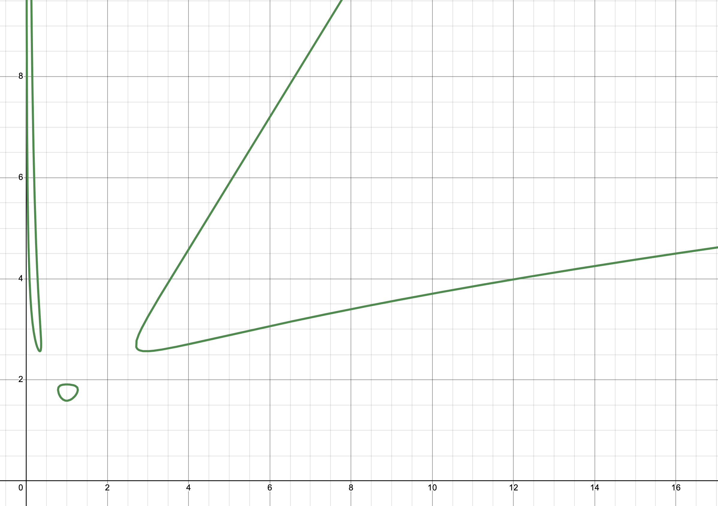
Figure 2: The positive zero set of $f=1+x^{4}-xy^{2}-x^{3}y^{2}+0.76x^{2}y^{3}$ has three connected components.

Remark 7.9.

The assumption that the points do not belong to a line cannot be dropped: the curve defined by the polynomial $f(x_{1},x_{2})=(x_{1}-1)(x_{1}-2)(x_{1}-3)(x_{1}-4)$ has $4$ connected components in the positive orthant.

Appendix A Proof of Claim 4.6

We prove now the following claim which was used for proving Proposition 4.5. We keep notations used in this latter proof.

Claim (Restating of Claim 4.6).

For all $(y_{1},\ldots,y_{k})\in{{\mathscr{C}}_{D}^{\nu}}$, we have

$$\det(J)=\gamma\left(\prod_{a\in\operatorname{\mathcal{A}}}\langle B_{a},y\rangle^{-1+\sum_{p=1}^{k-1}\lambda_{a,p}}\right)\cdot P_{{\mathrm{A}}}(y)\cdot\left(\sum_{j=1}^{k}y_{i}^{2}\right)\cdot\left(\sum_{a\in\operatorname{\mathcal{A}}}h_{a}\langle B_{a},y\rangle\right)$$

where $\gamma$ is a non-zero real constant which does not depend on $y$.

Proof.

We will use different notations during this proof. We will denote by $\lvert\textrm{M}\rvert$ the determinant of the matrix M. Moreover $\textrm{M}_{I}^{J}$ is the submatrix from $\mathrm{M}$ we get by keeping the rows from $I$ and the columns from $J$. We will also similarly use $\mathrm{M}_{I}$ and $\mathrm{M}^{J}$. Then $\mathrm{M}_{\setminus i}$ and $\mathrm{M}^{\setminus j}$ means that we remove respectively the $i$th row and the $j$th column from $\mathrm{M}$.

We will apply several times Laplace expansion, so for $I\subset[1,p]$ let us denote by $\varepsilon(I)$ the value $\sum_{i\in I}i+\sum_{i=1}^{\lvert I\rvert}i$. To be coherent with this previous convention, we will use here an ordering of $\operatorname{\mathcal{A}}=\{a_{1},\ldots,a_{n+k+1}\}$ (starting the numerotation by $1$ and not $0$ as in the remainder of the paper). Thus for $I\subset\operatorname{\mathcal{A}}$, we will write $\varepsilon(I)$ for $\varepsilon(\{j\in[1,n+k+1]\mid a_{j}\in I\})$.

Finally, if $V\in M_{p+q,q}$ is a matrix Gale dual to a matrix $U\in M_{p,p+q}$, then we note $\gamma_{U}$ be the constant verifying that for all $I\subset[1,p+q]$ with $\lvert I\rvert=q$, $\lvert V_{I}\rvert=(-1)^{\varepsilon(^{c}I)}\cdot\gamma_{V}\cdot\lvert U^{{}^{c}I}\rvert$.

We will expand the expression of $\det{J}$ to get the right hand side of the claimed identity. We have since $B_{a}=c_{a}D_{a}$,

$$\frac{\partial\phi_{i}}{\partial y_{j}}=\sum_{a\in\operatorname{\mathcal{A}}}\frac{\lambda_{a,i}\mathrm{D}_{a,j}}{\langle D_{a},y\rangle}\prod_{\ell\in\operatorname{\mathcal{A}}}\langle D_{\ell},y\rangle^{\lambda_{\ell,i}}=\sum_{a\in\operatorname{\mathcal{A}}}\frac{\lambda_{a,i}\mathrm{B}_{a,j}}{\langle B_{a},y\rangle}\prod_{\ell\in\operatorname{\mathcal{A}}}\langle D_{\ell},y\rangle^{\lambda_{\ell,i}}.$$

So the matrix $\phi=\left(\frac{\partial\phi_{i}}{\partial y_{j}}\right)\in M_{k-1,k}(\operatorname{\mathbb{R}})$ equals

$$\text{Diag}_{i}\left(\prod_{\ell\in\operatorname{\mathcal{A}}}\langle D_{\ell},y\rangle^{\lambda_{\ell,i}}\right)\cdot\lambda^{T}\cdot\text{Diag}_{a}\left(1/{\langle B_{a},y\rangle}\right)\cdot\mathrm{B}.$$

Let us define $G\operatorname{\stackrel{{\scriptstyle\text{def}}}{{=}}}\left(\prod_{\ell\in\operatorname{\mathcal{A}}}c_{\ell}^{1-\sum_{p=1}^{k-1}\lambda_{\ell,p}}\right)\left(\prod_{\ell\in\operatorname{\mathcal{A}}}\langle B_{\ell},y\rangle^{-1+\sum_{p=1}^{k-1}\lambda_{\ell,p}}\right)$.

By expanding the last row of $J$ and using Cauchy-Binet formula, we obtain

$$(\det{J})/G$$

$$= \sum_{i=1}^{k}(-1)^{i+k}y_{i}\sum_{I,\lvert I\rvert=k-1}\lvert\lambda_{I}\rvert\cdot\lvert\mathrm{B}_{I}^{\setminus i}\rvert\cdot\prod_{\ell\notin I}\langle B_{\ell},y\rangle$$

$$= \sum_{i=1}^{k}\sum_{I,\lvert I\rvert=k-1}(-1)^{i+k+\varepsilon(^{c}I)}y_{i}\gamma_{\lambda}\cdot\lvert{{\mathrm{A}}^{h}}^{{}^{c}I}\rvert\cdot\lvert\mathrm{B}_{I}^{\setminus i}\rvert\cdot\prod_{\ell\notin I}\langle B_{\ell},y\rangle$$

$$= \sum_{i=1}^{k}\sum_{\sigma,\lvert\sigma\rvert=n}\sum_{\begin{subarray}{c}u\neq v\in\operatorname{\mathcal{A}}\setminus\sigma\\ \sigma uv\operatorname{\stackrel{{\scriptstyle\text{def}}}{{=}}}\sigma\cup\{u\}\cup\{v\}\end{subarray}}(-1)^{i+k+\varepsilon(\sigma uv)}(-1)^{n+\lvert\{j\in\sigma\mid j\text{ between }u\text{ and }v\}\rvert+\mathbb{1}_{u<v}}$$

$$\quad\quad\quad\quad\quad\quad\cdot y_{i}\gamma_{\lambda}\cdot\lvert\hat{{\mathrm{A}}}^{\sigma}\rvert\cdot h_{u}\cdot\lvert\mathrm{B}_{{}^{c}\sigma uv}^{\setminus i}\rvert\cdot\prod_{\ell\in\sigma uv}\langle B_{\ell},y\rangle.$$

The last equality follows from Laplace expansion applied to the first and the last row of ${\mathrm{A}}^{h}$. Let us consider $\tilde{\mathrm{B}}_{i,^{c}\sigma u}$ being the matrix $\mathrm{B}_{{}^{c}\sigma u}$ where the column $i$ is replaced by the column $\mathrm{B}_{{}^{c}\sigma u}\cdot y^{T}$. Laplace expansion along the $i^{\text{th}}$ column also gives (denoting $\sigma\cup\{u\}$ by $\sigma u$)

$$y_{i}\lvert\mathrm{B}_{{}^{c}\sigma u}\rvert =\lvert\tilde{\mathrm{B}}_{i,^{c},\sigma u}\rvert$$

$$=\sum_{t=1}^{k}y_{t}\sum_{v\notin\sigma u}(-1)^{i+1+\varepsilon(\{v\})+\mathbb{1}_{u<v}+\lvert\{j\in\sigma\mid j<v\}\rvert}\lvert\mathrm{B}^{\setminus i}_{(^{c}\sigma u)\setminus v}\rvert\mathrm{B}_{v,t}$$

$$=\sum_{v\notin\sigma u}(-1)^{i+1+\varepsilon(\{v\})+\mathbb{1}_{u<v}+\lvert\{j\in\sigma\mid j<v\}\rvert}\lvert\mathrm{B}^{\setminus i}_{(^{c}\sigma u)\setminus v}\rvert\cdot\langle B_{v},y\rangle.$$

Consequently,

$$(\det{J})/(G\cdot\sum_{i=1}^{k}y_{i}^{2})$$

$$= \sum_{\sigma,\lvert\sigma\rvert=n}\sum_{u\notin\sigma}(-1)^{k+\varepsilon(\sigma u)+\lvert\{j\in\sigma\mid j<u\}\rvert}$$

$$\quad\quad\quad\quad\quad\quad\cdot\gamma_{\lambda}\cdot\lvert\hat{{\mathrm{A}}}^{\sigma}\rvert\cdot h_{u}\cdot\lvert\mathrm{B}_{{}^{c}\sigma u}\rvert\cdot\prod_{\ell\in\sigma u}\langle B_{\ell},y\rangle$$

$$= \sum_{\sigma,\lvert\sigma\rvert=n}\sum_{u\notin\sigma}(-1)^{k+\lvert\{j\in\sigma\mid j<u\}\rvert}$$

$$\quad\quad\quad\quad\quad\quad\cdot\gamma_{\lambda}\gamma_{B}\cdot\lvert\hat{{\mathrm{A}}}^{\sigma}\rvert\cdot h_{u}\cdot\lvert{\mathrm{A}}^{\sigma u}\rvert\cdot\prod_{\ell\in\sigma u}\langle B_{\ell},y\rangle$$

$$= \sum_{\sigma,\lvert\sigma\rvert=n}\sum_{u\notin\sigma}\sum_{t\in\sigma u}(-1)^{k+\lvert\{j\in\sigma\mid j<u\}\rvert+\lvert\{j\in\sigma\mid j<t\}\rvert+\mathbb{1}_{u<t}}$$ (17)

$$\quad\quad\quad\quad\quad\quad\cdot\gamma_{\lambda}\gamma_{B}\cdot\lvert\hat{{\mathrm{A}}}^{\sigma}\rvert\cdot h_{u}\cdot\lvert\hat{{\mathrm{A}}}^{\sigma u\setminus\{t\}}\rvert\cdot\prod_{\ell\in\sigma u}\langle B_{\ell},y\rangle.$$

Consider the terms of the previous sum when $t\neq u$ and doing the change of variables $\sigma^{\prime}=\sigma\cup\{u\}\setminus\{t\}$,

$$\sum_{\sigma,\lvert\sigma\rvert=n}\sum_{u\notin\sigma}\sum_{t\in\sigma}(-1)^{k+\lvert\{j\in\sigma\mid j<u\}\rvert+\lvert\{j\in\sigma\mid j<t\}\rvert+\mathbb{1}_{u<t}}$$

$$\quad\quad\quad\quad\quad\quad\cdot\gamma_{\lambda}\gamma_{B}\cdot\lvert\hat{{\mathrm{A}}}^{\sigma}\rvert\cdot h_{u}\cdot\lvert\hat{{\mathrm{A}}}^{\sigma u\setminus\{t\}}\rvert\cdot\prod_{\ell\in\sigma u}\langle B_{\ell},y\rangle$$

$$= \sum_{\sigma^{\prime},\lvert\sigma^{\prime}\rvert=n}\sum_{u\in\sigma^{\prime}}\sum_{t\notin\sigma^{\prime}}(-1)^{k+\lvert\{j\in\sigma^{\prime}\mid j<u\}\rvert+\lvert\{j\in\sigma^{\prime}\mid j<t\}\rvert+\mathbb{1}_{t<u}}$$

$$\quad\quad\quad\quad\quad\quad\cdot\gamma_{\lambda}\gamma_{B}\cdot\lvert\hat{{\mathrm{A}}}^{\sigma^{\prime}\cup\{t\}\setminus\{u\}}\rvert\cdot h_{u}\cdot\lvert\hat{{\mathrm{A}}}^{\sigma^{\prime}}\rvert\cdot\prod_{\ell\in\sigma^{\prime}\cup\{t\}}\langle B_{\ell},y\rangle$$

$$= \sum_{\sigma^{\prime},\lvert\sigma^{\prime}\rvert=n}\sum_{u\in\sigma^{\prime}}(-1)^{k+\lvert\{j\in\sigma^{\prime}\mid j<u\}\rvert}\cdot\gamma_{\lambda}\gamma_{B}h_{u}\cdot\lvert\hat{{\mathrm{A}}}^{\sigma^{\prime}}\rvert\cdot\prod_{\ell\in\sigma^{\prime}}\langle B_{\ell},y\rangle$$ (18)

$$\quad\quad\quad\quad\quad\quad\sum_{t\notin\sigma^{\prime}}(-1)^{\lvert\{j\in\sigma^{\prime}\mid j<t\}\rvert+\mathbb{1}_{t<u}}\left\lvert\hat{{\mathrm{A}}}^{\sigma^{\prime}\cup\{t\}\setminus\{u\}}\right\rvert\langle B_{t},y\rangle.$$

Let us consider the inside sum

$$\sum_{t\notin\sigma^{\prime}}(-1)^{\lvert\{j\in\sigma^{\prime}\mid j<t\}\rvert+\mathbb{1}_{t<u}}\left\lvert\hat{{\mathrm{A}}}^{\sigma^{\prime}\cup\{t\}\setminus\{u\}}\right\rvert\langle B_{t},y\rangle$$

$$= (-1)\sum_{t\notin\sigma^{\prime}}\left\lvert\hat{{\mathrm{A}}}^{\{t\}}\mid\hat{{\mathrm{A}}}^{\sigma^{\prime}\setminus\{u\}}\right\rvert\langle B_{t},y\rangle$$

$$= -\left(\sum_{t\in\operatorname{\mathcal{A}}}\left\lvert\hat{{\mathrm{A}}}^{\{t\}}\mid\hat{{\mathrm{A}}}^{\sigma^{\prime}\setminus\{u\}}\right\rvert\langle B_{t},y\rangle\right)+((-1)^{\lvert\{j\in\sigma^{\prime}\mid j<u\}\rvert}\cdot\lvert\hat{{\mathrm{A}}}^{\sigma^{\prime}}\rvert\cdot\langle B_{u},y\rangle)$$

$$= \left(\sum_{\ell=1}^{n}(-1)^{\ell+1}\left\lvert\hat{{\mathrm{A}}}^{\sigma^{\prime}\setminus\{u\}}_{\setminus\{\ell\}}\right\rvert\sum_{t\in\operatorname{\mathcal{A}}}t_{\ell}\langle B_{t},y\rangle\right)+(-1)^{\lvert\{j\in\sigma^{\prime}\mid j<u\}\rvert}\cdot\lvert\hat{{\mathrm{A}}}^{\sigma^{\prime}}\rvert\cdot\langle B_{u},y\rangle$$

$$= \left(\sum_{\ell=1}^{n}(-1)^{\ell+1}\left\lvert\hat{{\mathrm{A}}}^{\sigma^{\prime}\setminus\{u\}}_{\setminus\{\ell\}}\right\rvert\langle A_{\ell}\cdot B,y\rangle\right)+(-1)^{\lvert\{j\in\sigma^{\prime}\mid j<u\}\rvert}\cdot\lvert\hat{{\mathrm{A}}}^{\sigma^{\prime}}\rvert\cdot\langle B_{u},y\rangle$$

$$= (-1)^{\lvert\{j\in\sigma^{\prime}\mid j<u\}\rvert}\cdot\lvert\hat{{\mathrm{A}}}^{\sigma^{\prime}}\rvert\cdot\langle B_{u},y\rangle.$$

Reinjecting the last expression in 18, we can now compute 17 as the sum of the case $t=u$ and of 18:

$$(\det{J})/(G\sum_{i=1}^{k}y_{i}^{2})$$

$$= \sum_{\sigma,\lvert\sigma\rvert=n}\sum_{u\notin\sigma}(-1)^{k}\cdot\gamma_{\lambda}\gamma_{B}\cdot\lvert\hat{{\mathrm{A}}}^{\sigma}\rvert^{2}\cdot h_{u}\cdot\prod_{\ell\in\sigma u}\langle B_{\ell},y\rangle$$

$$\quad\quad\quad\quad\quad\quad+\sum_{\sigma^{\prime},\lvert\sigma^{\prime}\rvert=n}\sum_{u\in\sigma^{\prime}}(-1)^{k}\cdot\gamma_{\lambda}\gamma_{B}h_{u}\cdot\lvert\hat{{\mathrm{A}}}^{\sigma^{\prime}}\rvert^{2}\cdot\langle B_{u},y\rangle\cdot\prod_{\ell\in\sigma^{\prime}}\langle B_{\ell},y\rangle$$

$$= \sum_{\sigma,\lvert\sigma\rvert=n}\sum_{a\in\operatorname{\mathcal{A}}}(-1)^{k}\cdot\gamma_{\lambda}\gamma_{\mathrm{B}}\cdot\lvert\hat{{\mathrm{A}}}^{\sigma}\rvert^{2}\cdot h_{a}\cdot\langle B_{a},y\rangle\cdot\prod_{\ell\in\sigma}\langle B_{\ell},y\rangle$$

$$= (-1)^{k}\gamma_{\lambda}\gamma_{\mathrm{B}}\cdot P_{{\mathrm{A}}}\cdot\left(\sum_{a\in\operatorname{\mathcal{A}}}h_{a}\langle B_{a},y\rangle\right).$$

That is the claimed identity. ∎

References

- [1] Frederic Bihan. Polynomial systems supported on circuits and dessins d’enfants. Journal of the London Mathematical Society, 75(1):116–132, 2007.
- [2] Frédéric Bihan. Topologie des variétés creuses. PhD thesis, Habilitation thesis, Université de Savoie, France, 2011.
- [3] Frédéric Bihan and Alicia Dickenstein. Descartes? rule of signs for polynomial systems supported on circuits. International Mathematics Research Notices, 2017(22):6867–6893, 2017.
- [4] Frédéric Bihan, Alicia Dickenstein, and Jens Forsgård. Optimal descartes? rule of signs for systems supported on circuits. Mathematische Annalen, 381(3):1283–1307, 2021.
- [5] Frédéric Bihan, Alicia Dickenstein, and Magalí Giaroli. Sign conditions for the existence of at least one positive solution of a sparse polynomial system. Advances in Mathematics, 375:107412, 2020.
- [6] Frédéric Bihan, J Maurice Rojas, and Frank Sottile. On the sharpness of fewnomial bounds and the number of components of fewnomial hypersurfaces. In Algorithms in algebraic geometry, pages 15–20. Springer, 2008.
- [7] Frederic Bihan, J Maurice Rojas, and Casey E Stella. Faster real feasibility via circuit discriminants. In Proceedings of the 2009 international symposium on Symbolic and algebraic computation, pages 39–46, 2009.
- [8] Frédéric Bihan and Frank Sottile. New fewnomial upper bounds from gale dual polynomial systems. Moscow mathematical journal, 7(3), 2007.
- [9] Frédéric Bihan and Frank Sottile. Gale duality for complete intersections. In Annales de l’institut Fourier, volume 58-3, pages 877–891, 2008.
- [10] Frederic Bihan and Frank Sottile. Betti number bounds for fewnomial hypersurfaces via stratified morse theory. Proceedings of the American Mathematical Society, 137(9):2825–2833, 2009.
- [11] Anders Bjorner, Anders Björner, Michel Las Vergnas, Bernd Sturmfels, Neil White, and Gunter M Ziegler. Oriented matroids. Number 46 in Encyclopedia of Mathematics and its Applications. Cambridge University Press, 1999.
- [12] Gheorghe Craciun, Luis David García-Puente, and Frank Sottile. Some geometrical aspects of control points for toric patches. In International Conference on Mathematical Methods for Curves and Surfaces, pages 111–135. Springer, 2008.
- [13] Jens Forsgård. Defective dual varieties for real spectra. Journal of Algebraic Combinatorics, 49(1):49–67, 2019.
- [14] Jens Forsgård, Mounir Nisse, and J Maurice Rojas. New subexponential fewnomial hypersurface bounds. arXiv preprint arXiv:1710.00481, 2017.
- [15] Israel M Gelfand, Mikhail M Kapranov, and Andrei V Zelevinsky. Discriminants, resultants and multidimensional determinants. Modern Birkhuser Classics, Birkhuser, Boston, MA, 1994.
- [16] Mark Goresky and Robert MacPherson. Stratified morse theory. Springer, 1988.
- [17] David GC Handron. Generalized billiard paths and morse theory for manifolds with corners. Topology and its Applications, 126(1-2):83–118, 2002.
- [18] Ilia Itenberg, Grigory Mikhalkin, and Eugenii I Shustin. Tropical algebraic geometry, volume 35. Springer Science & Business Media, 2009.
- [19] Askold G Khovanskiĭ. Fewnomials, volume 88. American Mathematical Soc., 1991.
- [20] Tien-Yien Li, J Maurice Rojas, and Xiaoshen Wang. Counting real connected components of trinomial curve intersections and m-nomial hypersurfaces. Discrete & Computational Geometry, 30(3):379–414, 2003.
- [21] James G Oxley. Matroid theory, volume 3. Oxford University Press, USA, 2006.
- [22] Daniel Perrucci. Some bounds for the number of components of real zero sets of sparse polynomials. Discrete & Computational Geometry, 34(3):475–495, 2005.
- [23] Ata Pir and Frank Sottile. Irrational toric varieties and secondary polytopes. arXiv preprint arXiv:1807.05919, 2018.
- [24] Elisa Postinghel, Frank Sottile, and Nelly Villamizar. Degenerations of real irrational toric varieties. Journal of the London Mathematical Society, 92(2):223–241, 2015.
- [25] Jean-Jacques Risler. Construction d?hypersurfaces réelles [d?apres viro]. Séminaire Bourbaki, 1992:93, 1992.
- [26] J. Maurice Rojas and Korben Rusek. A-discriminants for complex exponents, and counting real isotopy types. arXiv:1612.03458, 2016.
- [27] Frank Sottile. Real solutions to equations from geometry, volume 57. American Mathematical Soc., 2011.
- [28] SA Vakhrameev. Morse lemmas for smooth functions on manifolds with corners. Journal of Mathematical Sciences, 100(4):2428–2445, 2000.
- [29] Oleg Y. Viro. Constructing real algebraic varieties with prescribed topology. Thesis, LOMI, Leningrad., 1983. An english translation by the author can be found in https://arxiv.org/pdf/math/0611382.pdf.
- [30] Oleg Y. Viro. Gluing of plane real algebraic curves and constructions of curves of degrees 6 and 7. In Topology, pages 187–200. Springer, 1984.
- [31] Dominic JA Welsh. Matroid theory. Courier Corporation, 2010.
- [32] Günter M Ziegler. Lectures on polytopes, volume 152. Springer Science & Business Media, 2012.