Long-term Causal Effects Estimation via Latent Surrogates Representation Learning
Abstract
Estimating long-term causal effects based on short-term surrogates is a significant but challenging problem in many real-world applications such as marketing and medicine. Most existing methods estimate causal effects in an idealistic and simplistic manner - disregarding unobserved surrogates and treating all short-term outcomes as surrogates. However, such methods are not well-suited to real-world scenarios where the partially observed surrogates are mixed with the proxies of unobserved surrogates among short-term outcomes. To address this issue, we develop our flexible method called LASER to estimate long-term causal effects in a more realistic situation where the surrogates are either observed or have observed proxies. In LASER, we employ an identifiable variational autoencoder to learn the latent surrogate representation by using all the surrogate candidates without the need to distinguish observed surrogates or proxies of unobserved surrogates. With the learned representation, we further devise a theoretically guaranteed and unbiased estimation of long-term causal effects. Extensive experimental results on the real-world and semi-synthetic datasets demonstrate the effectiveness of our proposed method.
keywords:
Long-term causal effects , Surrogates , LASER , Identifiable variational autoencoderPACS:
0000 , 1111MSC:
0000 , 1111[inst1]organization=School of Computer Science, Guangdong University of Technology,city=Guangzhou, country=China
[inst2]organization=School of Computing and Augmented Intelligence, Arizona State University,city=Tempe, state=AZ, country=USA
[inst3]organization=Didi Chuxing,city=Beijing, country=China
1 Introduction
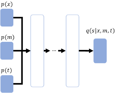
Estimating long-term causal effects is an important but challenging problem in many fields, from marketing (e.g., long-term revenue affected by high/low quality of advertising [1]), to medicine (e.g., taking years of follow-up to fully reveal mortality in acquired immunodeficiency syndrome drug clinical trials [2]). A key challenge in estimating long-term causal effects is the expense of conducting a long-time experiment to obtain a long-term outcome. Existing methods [3, 4, 5, 6] try to solve this problem by conducting short-time experiments and utilizing short-term outcomes as surrogates to estimate the long-time outcomes, which is much cheaper and more feasible, as shown in Figure 1 and Example 1.1.
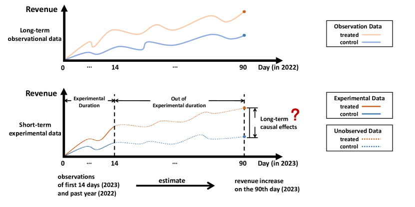
Example 1.1.
In the example illustrated in Figure 1, to increase customer loyalty and revenue in the next quarter of 2023, a ride-hailing platform needs to evaluate long-term campaign strategies such as a 90-day taxi promotion or advertising strategy. There are two ways to estimate the long-term effects of the promotion on revenue. One way is to conduct a 90-day random control experiment, and another way is to conduct an only-14-days experiment and to collect historical 90-day data available on the platform in the previous year. Comparing the two ways, the first will result in unaffordable marketing costs, while the second is considerably more feasible and acceptable to the ride-hailing platform.
Existing methods try to estimate long-term causal effects of treatment by utilizing surrogates, e.g., predicting the 90-day revenue increase of a promotion strategy by using users’ first 14-day usage frequency in Example 1.1. Athey et al. [5] propose Surrogate Index (SInd), a long-term outcome predictor given surrogates and covariates to estimate long-term causal effects based on the surrogacy assumption. Kallus et al. [7] propose an estimator based on flexible machine learning methods to estimate nuisance parameters. Cheng et al. [6] concentrate on time-dependent surrogates and employ an Recurrent Neural Network (RNN) with double heads to capture nonlinearity between surrogates and long-term outcomes. By utilizing the surrogates’ information related to the long-term outcome in observational data, these methods propose different types of estimators for long-term causal effects.
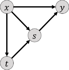
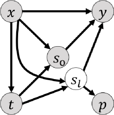
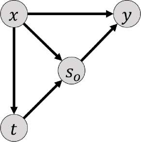
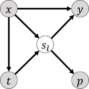
In many real-world scenarios, however, without considering unobserved surrogates and by treating all short-term outcomes as surrogates, existing methods estimate long-term effects in an idealistic and simplistic way like Figure 2(a). As shown in Example 1.1 and Figures 2(b), 2(c), in estimating the long-term effects of a promotion on the revenue on the ride-hailing platform, there exist unobserved surrogates (e.g., user habituation directly caused by the promotion) and lots of observed short-term variables, including the observed surrogates (e.g., regional empty taxi rate directly caused by the promotion) and noisy proxies of unobserved surrogates (e.g., users’ behaviors and users’ cost of calling taxis caused by user habituation). The long-term revenue heavily relies only on the and , but the can not be observed and the are indistinguishable from in multiple short-term outcomes. To work around this problem, existing works pose strong assumptions on the short-term outcomes and by excluding to obtain unbiased long-term outcome , which is often impractical in real-world scenarios.
To tackle the challenges of unobserved surrogates and indistinguishable observed short-term outcomes ( and ), we propose our method to identify long-term causal effects using LAtent SurrogatE Representation learning (LASER in short). Our method does not require accessing all valid surrogates nor distinguishing the observed surrogates from short-term outcomes. The generalized causal model is given in Figure 2(b). In detail, we aim to learn the predictive surrogate representation based on an identifiable variational auto-encoder (iVAE). Given the learned representation, the long-term causal effects can be directly estimated by classic methods, e.g., the Inverse Probability Weighting (IPW) method. We also extend our work to two special cases - we observe all valid surrogates and we only observe proxies. In summary, our contributions are as follows:
-
1.
We propose our method LASER to overcome the challenge of estimating long-term causal effects in the case that the valid surrogates are partially or even completely unobserved but noisy proxies of latent surrogates can be observed.
-
2.
Without the need to distinguish the observed surrogates and proxies of latent surrogates from short-term outcomes, we learn the surrogate representation in a unified way and provide the theoretically guaranteed identification of long-term causal effects.
-
3.
We provide extensive experimental results on both real-world datasets and semi-synthetic datasets which demonstrate the effectiveness of our proposed method.
2 Related Works
Related to Traditional Causal Inference: The traditional causal inference has been studied mainly in two languages: the graphical models [8] and the potential outcome framework [9]. The most related method is the propensity score method in the potential outcome framework, e.g., IPW method [10, 11]. Moreover, several neural networks-based works [12, 13, 14, 15, 16, 17] have been proposed, which mainly aim to learn a balanced representation or recover disentangled latent confounders. Different from these works above, we focus on the long-term setting and learn the latent surrogate representation instead of balanced representation or confounders.
Related to Surrogates: For many years, many works are interested in what is a valid surrogate that can reliably predict the long-term causal effects on treatment. Prentice criteria [3] is the first criteria proposing statistical surrogate condition that only requires the treatment and long-term outcome are independent conditioning on the surrogate. Based on the principal stratification framework, principal criteria [4] additionally consider the property of causal necessity, i.e., the absence of the causal effects on the surrogate indicates the absence of causal effects on the long-term outcome. Based on the language of graphical models, strong surrogate criteria [18] argue that a surrogate is valid for the effect of a treatment on the long-term outcome if and only if treatment is an instrument for the effects of the surrogates on long-term outcome. Causal effect predictiveness (CEP) [19] was introduced to evaluate a principal surrogate. However, the surrogate paradox still exists when these criteria hold, which means the treatment has a positive effect on surrogates but a negative effect on the long-term outcome. Consistent surrogate and several variants [20, 21, 22] propose various conditions for testing a valid surrogate to avoid surrogate paradox.
Moreover, many works have been proposed to estimate long-term causal effects based on surrogates. SInd [5] combines multiple surrogates to robustly estimate long-term causal effects. Cheng et al. [6] propose the Long-Term Effect Estimation method (LTEE) by adapting an RNN with double heads to learn the time-dependent link between time-dependent surrogates and the long-term outcome. Kallus et al. [7] propose Efficient Estimation for Treatment Effects (EETE) and analyze the benefit of surrogates in estimating causal effects and applies a nuisance estimator to long-term causal effects estimation. Some works [23, 24] also focus on the latent confounder problem in the long-term setting and propose causal effects estimators without the unconfoundedness assumption. Different from these works above, we consider the observed short-term outcomes including observed surrogates and the proxies of latent surrogates, and in this case, these surrogate criteria do not hold, including traditional surrogacy assumption.
Related to Variational Auto-encoders: Our work is also related to the variational auto-encoders (VAE) [25, 26]. The VAE attempts to approximate an intractable posterior inference in the presence of latent variables. Its variants include -VAE [27], Hilbert-Schmidt information criterion-constrained VAE [28], -VAE [29], coupled conditional VAE [30] and so on. However, these variants do not guarantee the identifiability of latent variables. A recent variant, called identifiable VAE (iVAE) [31], approximates the posterior with additional supervised information to ensure recovery of the true latent variables. Recently, Yao et.al [32] borrow the idea of iVAE and propose the latent temporally causal processes estimation method for modeling causal latent processes. In this paper, our method absorbs the core of iVAE, which not only learns the latent surrogate representation to guarantee the unbiased causal effects estimation but also provides the identification.
3 Problem Definition
Let be the covariates (also known as pre-treatment features or confounders). Let denote a binary treatment, where indicates a unit receives the treatment (treated) and indicates a unit receives no treatment (control). Let denote latent surrogates and denote the observed surrogates, with the entire set of valid surrogates represented by concatenating where . Let denote the proxies of latent surrogates, and for simplicity, we also denote the observed short-term outcomes as the mixture of observed surrogates and proxies of latent surrogates . Let be the long-term outcome. Let and denote the potential outcome under the treatment group and control group, respectively. Note that we can only observe one of the potential outcomes, and then .
In this paper, given a set of historical data (observational data) , our goal is to estimate the average treatment effects (ATE) on the target population, i.e., experimental data, as follows:
| (1) |
where means do-operation [33].
In this work, our assumptions include Stable Unit Treatment Value Assumption (SUTVA), Overlap, and Unconfoundedness assumptions which are widely adopted in existing casual inference methods [10, 5, 6, 7, 16]. We further assume the following assumptions hold:
Assumption 3.1.
(Comparability Assumption [5]). Given the covariates and the valid surrogates , the conditional distribution of in observational data is identical to that in experimental data. Formally,
where and denote the distribution on observational and experimental data, respectively.
Assumption 3.2.
(Partially Latent Surrogacy Assumption). Given the covariates and the valid surrogates, including the observed surrogates and the latent surrogates of which we only have the proxies , the treatment is independent of the long-term outcome . Formally,
Assumption 3.1 places the connection between observational and experimental data on the conditional distribution of . It allows inferring in experimental data by making use of in observational data.
Assumption 3.2 is the core assumption in our paper, which implies that given covariates the valid surrogates contain all causal information between the treatment and the long-term outcome. This assumption does not require full observation of the valid surrogates and even does not require observing one of the surrogates as long as the proxies are observed. Please note that this assumption is much weaker than the original surrogacy assumption in [5], i.e., , which requires full observation of surrogates to totally block the causal path between the treatment and the long-term outcome.
It is challenging to estimate long-term causal effects when surrogates are partially observed and mixed with noisy proxies, which, however, is a very common scenario in reality (see Example 1.1). Surprisingly, we find that noisy proxies of latent surrogates can still be useful in estimating long-term causal effects. Thus, we develop a representation learning method to jointly process noisy proxies and partially observed surrogates (see Section 4) and provide theoretically guaranteed and unbiased estimation (see Section 5).
4 Methodology
In this section, we aim to devise a practical LAtent SurrogatEs Representation learning method (LASER in short) to construct a predictive surrogate representation and further estimate the long-term causal effects, jointly taking the mixture of observed surrogates and proxies of latent surrogates as inputs. LASER generally consists of the following two steps: the iVAE-based representation learning step and the IPW-based causal effects estimation step.
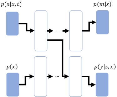
In the representation learning step, we employ iVAE to construct a predictive surrogate representation from the mixture of observed surrogates and the proxies of latent surrogates as inputs. Specifically, considering the causal graph in Figure 2(b), we reconstruct from , by incorporating and as additional supervised information to approximate the conditional prior . Such additional supervised information not only improves the quality of the learned representations but also guarantees the identifiability of the model.
We further devise an end-to-end neural network architecture for the representation learning as shown in Figure 3. The design of inference and generative network follows the distribution factorization as shown in Figure 2(b). For the inference network, the covariates and the treatment as additional supervised information are input together with to approximate appropriate prior , which importantly guarantees the power of approximation. For the generative network, besides the approximation of posterior , we also employ an MultiLayer Perceptron (MLP) to approximate . Considering the partially latent surrogacy assumption 3.2, training such an MLP at the same time will not only encourage the learned approximating the valid surrogates but also avoid the extra regression step of fitting after learning the surrogates .
Following existing VAE-based works, we choose the prior as standard Gaussian distribution, which can be extended to exponential family distributions as discussed in Section 5, and thus each of the dimensions of has two sufficient statistics, the mean and variance:
| (2) |
where is the parameter that determines the dimensions of surrogates .
In the inference network, the variational approximation of the posterior is defined as:
| (3) |
where and are the mean and variance of the Gaussian distribution parametrized by the inference network.
In the generative network, for a continuous outcome, we parametrize the probability distribution as a Gaussian distribution with its mean given by an MLP and a fixed variance . For a discrete outcome, we use a Bernoulli distribution parametrized by an MLP similarly:
| (4) | ||||
where for the continuous case and are the mean of the Gaussian distribution parametrized by the generative network similar to inference network, and and are the fixed variance of Gaussian distribution, and for the discrete case and are the mean of Bernoulli distribution similarly parametrized by the network.
We can now form the objective function for the inference and generative networks, consisting of the negative variational Evidence Lower BOund (ELBO) of the graphical model and the negative marginal log-likelihood of for reconstruction as follows:
| (5) | ||||
where and are the empirical data distributions given by dataset and respectively. The ELBO derivation is given in D.
In the causal effects estimation step, we simply utilize the IPW method to estimate the long-term causal effects. Specifically, given experimental data , we estimate the long-term causal effects as follows:
| (6) |
where is the output of the neural networks with input and denotes the propensity score .
It is worth noting that LASER does not need to distinguish between observed surrogates and proxies of latent surrogates within the mixed short-term outcomes. Instead, we use all the observed short-term outcomes, including and , to learn the complete surrogates and . Our method provides a unified way to process both the surrogates and proxies of latent surrogates. In the next section, we will discuss the identifiability to guarantee the correctness of our model.
5 Theoretical Analysis
In this section, we present the identifiability of our model and long-term causal effects. Note that if we correctly identify the valid surrogates, the long-term causal effects can be identified based on the IPW method.
For simplicity, we externally define the proxies of without noise as . Thus the mixture can be viewed as , which only consists of the proxies. In this way, both and can be considered as the latent variables, while both and can be observed.
Let be the parameters on of the following conditional generative models:
| (7) | ||||
where we define the following injective function :
| (8) |
in which we assume that is a conditional independent noise variable with probability density function , i.e., is mutually independent given . The proxies are allowed to have different practical meaning from the surrogates , but must be generated by and as valid proxies.
To specify the correlation between latent variables and observed variables , we assume the conditional distribution is conditional factorial with an exponential family distribution:
Assumption 5.1.
The correlation between and is characterized by:
| (9) | ||||
where is the base measure, is the normalizing constant, are sufficient statistics, and are the dependent parameters, and is the dimension of each sufficient statistic.
Assumption 5.1 specifies that the conditioning on is through an arbitrary function , which is crucial to make the latent surrogates identifiable. Note that the exponential families include many common distributions such as normal, exponential, gamma, beta, and Poisson, so Assumption 5.1 is not very restrictive. Such an assumption is widely used in VAE-based methods such as [14, 15, 31], and many of them usually further specify that the (conditional) prior is Gaussian. In our implementation, we also use Gaussian distribution as the conditional prior.
Then, we consider the following equivalence relation on the set of parameters from [31]:
Definition 5.2.
Let be the binary relation on defined as follows:
| (10) | ||||
where is a invertible matrix and is a vector, and is the domain of .
When the underlying model parameters can be recovered by perfectly fitting the conditional distribution , the joint distribution also can be recovered. This further implies the recovery of conditional prior and the recovery of latent surrogates (and noises ) up to some simple transformations. We conclude the identifiability of our model as follows:
Theorem 5.3.
Assume that the data we observed are generated following Eq. 7 and 8 and suppose Assumption 5.1 holds, and suppose the following conditions hold: (1) The sufficient statistics are differentiable almost everywhere, and are linearly independent on any subset of the domain of of measure greater than zero. (2) There exist distinct points such that the matrix
of size is invertible. Then the parameters are .
The proof is in A. Note that the last assumption in Theorem 5.3 requires there exist distinct points . The assumption is reasonable for two reasons. First, based on the Overlap assumption, i.e., , we only require that there exists distinct points . Further, in many scenarios the space of multivariate covariate is large enough so that we can easily collect sufficient enough different covariates.
Theorem 5.3 indicates that under mild assumptions, we can recover the and which are equal to a permutation (the matrix ) and a point-wise nonlinearity (in the form of and ) of the original latent surrogates and noises . Based on such recovered , we can further identify the long-term causal effects shown in the following theorem.
Theorem 5.4.
The proof is in B. Theorem 5.4 guarantees that given enough information that makes identifiable, the estimated ATE can also be identified under some mild assumptions which are usually assumed in causal inference. It theoretically guarantees the correctness of our model, providing a feasible technology of long-term causal effects estimation via learning latent surrogates. We also extend Theorem 5.4 to the following two special cases:
Corollary 5.5.
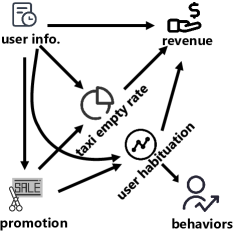
The proof is in C. Note that Figures 4(a) and 4(b) are only special cases under which our method LASER works well. In Figure 4(a), the proxies can be considered completely the same as observed surrogates, i.e., . In Figure 4(b), there are no observed surrogates and all observed short-term outcomes are proxies.
Corollary 5.5 indicates that regardless we observe the valid surrogates, the proxies of latent surrogates, or the mixed case, our method is able to estimate the long-term causal effects robustly, which guarantees practicability and flexibility of our representation learning based estimation method. In many real-world scenarios, we have a myriad of observed short-term variables, making it extremely difficult to distinguish between surrogates and proxies. Theorem 5.4 and Corollary 5.5 allow inferring long-term causal effects without considering the complex causal structure among short-term variables and identifying which are surrogates or proxies.
It is worth noting that the traditionally assumed causal graph like Figure 4(a) is also a special case of our model. It means that without testing whether the standard surrogacy assumption holds, our model can be an out-of-box tool to estimate long-term causal effects for many real-world applications.
6 Experiments
In this section, we validate the proposed LASER on real-world and semi-synthetic datasets. In detail, we verify the effectiveness of our method on the real-world dataset in Section 6.1 and we further evaluate the correctness of the theorem analysis with the help of the semi-synthetic datasets in Section 6.2 and 6.3. The real-world dataset is generously provided by the Chinese largest mobility technology platform and the semi-synthetic datasets are simulated based on the Infant Health and Development Program (IHDP) [34].
Baseline Methods: We consider several baseline methods including the state-of-the-art model based on neural networks like LTEE [6] and some statistical models like SInd [5] and Back-Door adjustment method (BD) [35]. Some baseline methods are proposed to deal with different settings, and we will clarify them as follows:
-
1.
LTEE [6]: LTEE uses an RNN with double heads to capture the relationship of time-dependent surrogates respectively in the treatment and control group, and then estimate CATE by the predicted long-term outcome. We use the code available at https://github.com/GitHubLuCheng/LTEE. It requires in observational data and in experimental data.
-
2.
SInd-Linear and SInd-MLP [5]: SInd uses a predictor named ”Surrogate Index” to predict the long-term outcome using surrogates, and the estimate CATE by the IPW method. We use linear regression (SInd-Linear) or an MLP (SInd-MLP) as the predictor to capture the relationship between surrogates and the long-term outcome. It requires in observational data and in experimental data.
-
3.
BD-Linear and BD-MLP [35]: We employ the back-door adjustment method using the fitted experimental long-term outcome by SInd. Specifically, we obtain the fitted long-term outcome of experimental data by SInd and perform two regressions of on the back-door adjustment set , i.e., and , using linear regressions (BD-Linear) or MLPs (BD-MLP). It requires in observational data and in experimental data.
-
4.
EETE [7]: EETE proposes an estimator and inferential method based on flexible machine learning methods to estimate nuisance parameters that appear in the influence functions. We implement its estimator in Python. To estimate causal effects, it requires in observational data and in experimental data.
Implementation details: We implement the basic version denoted by LASER and a modified version denoted by LASER-GRU. In LASER-GRU, we modify the extra MLP in the generative model to capture the time-dependent relationship between the long-term outcome and the specific surrogates that has the same practical meaning (e.g., the first days’ revenues when is the th day’s revenue). We apply a GRU by inputting to generate the time-dependent representation . Thus the modified extra MLP approximates: where . Our implementation is based on the code of iVAE. We choose the Leaky-ReLu as the activation function in our model and Adam is adopted to solve the optimization problem. All the experiments can be run on a single 8GB GPU of NVIDIA Tesla P40. Our code will be available after this paper is accepted.
Metric: We report the mean and the standard deviation of mean absolute percentage error (MAPE) of ATE on experimental data in -time runnings, where . The values presented are averaged over at least 5 replicated with different random seeds. The standard deviation is in the subscript.
6.1 Real-World Dataset
| Subject | Property | : Number | Exist In |
|---|---|---|---|
| dimension | : 15 | ||
| (all surrogates) | dimension | : 105 | |
| (revenues only) | dimension | : 14 | |
| dimension | : 1 | ||
| observational data (per strategy) | sample size | : 4592 | |
| experimental data (per strategy) | sample size | : 1008 |
| LASER | LASER-GRU | SInd-Linear | SInd-MLP | LTEE | EETE | BD-Linear | BD-MLP | ||
|---|---|---|---|---|---|---|---|---|---|
| Strategy | City | mean | mean | mean | mean | mean | mean | mean | mean |
| Strategy1 | All | 0.0179 | 0.0219 | 0.2070 | 0.1253 | 0.0151 | 0.0265 | 0.2086 | 0.1808 |
| A | 0.0306 | 0.0328 | 0.2406 | 0.1170 | 0.0562 | 0.0682 | 0.2246 | 0.1817 | |
| B | 0.0469 | 0.0563 | 0.1868 | 0.1855 | 0.1069 | 0.2112 | 0.2120 | 0.2060 | |
| C | 0.0232 | 0.0322 | 0.1481 | 0.1146 | 0.0839 | 0.0311 | 0.1961 | 0.2056 | |
| D | 0.0337 | 0.0373 | 0.1191 | 0.0926 | 0.0524 | 0.0923 | 0.1808 | 0.1923 | |
| Strategy2 | All | 0.0283 | 0.0167 | 0.2591 | 0.1584 | 0.0334 | 0.0636 | 0.1942 | 0.2346 |
| A | 0.0127 | 0.0301 | 0.2569 | 0.1300 | 0.0649 | 0.1091 | 0.2032 | 0.2470 | |
| B | 0.0686 | 0.0565 | 0.2160 | 0.2160 | 0.1447 | 0.0508 | 0.2048 | 0.2392 | |
| C | 0.0192 | 0.0412 | 0.2092 | 0.1753 | 0.0899 | 0.0234 | 0.2053 | 0.2428 | |
| D | 0.0420 | 0.0229 | 0.1906 | 0.1293 | 0.0645 | 0.0682 | 0.2038 | 0.2457 | |
| Strategy3 | All | 0.0471 | 0.0393 | 0.3301 | 0.2011 | 0.0476 | 0.1774 | 0.2170 | 0.2893 |
| A | 0.0384 | 0.0504 | 0.3595 | 0.1374 | 0.0601 | 0.2903 | 0.2289 | 0.2917 | |
| B | 0.0833 | 0.0773 | 0.2714 | 0.2754 | 0.1034 | 0.3425 | 0.2321 | 0.3101 | |
| C | 0.0583 | 0.0681 | 0.2600 | 0.1839 | 0.1251 | 0.1743 | 0.2341 | 0.3009 | |
| D | 0.0788 | 0.0638 | 0.2087 | 0.1480 | 0.1414 | 0.1130 | 0.2325 | 0.2881 | |
| Strategy4 | All | 0.0447 | 0.0311 | 0.3453 | 0.1892 | 0.0577 | 0.0474 | 0.2402 | 0.2828 |
| A | 0.0614 | 0.0726 | 0.3284 | 0.1216 | 0.1458 | 0.4315 | 0.2453 | 0.2852 | |
| B | 0.0872 | 0.0770 | 0.1858 | 0.2006 | 0.0934 | 0.1307 | 0.2420 | 0.2426 | |
| C | 0.0392 | 0.0204 | 0.2488 | 0.1744 | 0.1120 | 0.0441 | 0.2424 | 0.2583 | |
| D | 0.0512 | 0.0579 | 0.2849 | 0.1985 | 0.1266 | 0.0365 | 0.2446 | 0.2783 | |
| Strategy5 | All | 0.0428 | 0.0674 | 0.2685 | 0.1556 | 0.0432 | 0.0980 | 0.2463 | 0.2644 |
| A | 0.0532 | 0.0870 | 0.3340 | 0.0632 | 0.1183 | 0.0751 | 0.2503 | 0.2585 | |
| B | 0.3946 | 0.3804 | 0.2675 | 0.2767 | 0.3735 | 1.0166 | 0.2511 | 0.2583 | |
| C | 0.1000 | 0.0560 | 0.1699 | 0.1504 | 0.1131 | 0.1340 | 0.2477 | 0.2445 | |
| D | 0.1249 | 0.1159 | 0.2032 | 0.2139 | 0.3117 | 0.1310 | 0.2459 | 0.2541 |
| LASER | LASER-GRU | SInd-Linear | SInd-MLP | LTEE | EETE | BD-Linear | BD-MLP | ||
|---|---|---|---|---|---|---|---|---|---|
| Strategy | City | mean | mean | mean | mean | mean | mean | mean | mean |
| Strategy1 | All | 0.0185 | 0.0103 | 0.1814 | 0.0962 | 0.0256 | 0.0244 | 0.1804 | 0.1398 |
| A | 0.0146 | 0.0179 | 0.1384 | 0.1028 | 0.0449 | 0.0692 | 0.1591 | 0.1292 | |
| B | 0.0861 | 0.0718 | 0.1693 | 0.1542 | 0.0805 | 0.2100 | 0.1632 | 0.1743 | |
| C | 0.0312 | 0.0341 | 0.1096 | 0.0827 | 0.0616 | 0.0391 | 0.1498 | 0.1692 | |
| D | 0.0135 | 0.0221 | 0.0716 | 0.0481 | 0.0645 | 0.0913 | 0.1345 | 0.1650 | |
| Strategy2 | All | 0.0263 | 0.0295 | 0.2159 | 0.1281 | 0.0334 | 0.0634 | 0.1481 | 0.1622 |
| A | 0.0123 | 0.0151 | 0.1127 | 0.1030 | 0.0484 | 0.1109 | 0.1431 | 0.1409 | |
| B | 0.0449 | 0.0408 | 0.2069 | 0.2192 | 0.1509 | 0.0501 | 0.1520 | 0.1806 | |
| C | 0.0493 | 0.0522 | 0.1361 | 0.1096 | 0.0338 | 0.0231 | 0.1504 | 0.1819 | |
| D | 0.0529 | 0.0360 | 0.1261 | 0.0759 | 0.0719 | 0.0708 | 0.1482 | 0.1843 | |
| Strategy3 | All | 0.0146 | 0.0194 | 0.2704 | 0.1361 | 0.0388 | 0.1758 | 0.1604 | 0.2137 |
| A | 0.0397 | 0.0715 | 0.1716 | 0.1283 | 0.0626 | 0.2817 | 0.1615 | 0.1794 | |
| B | 0.0358 | 0.0834 | 0.2279 | 0.2180 | 0.0978 | 0.3576 | 0.1666 | 0.2409 | |
| C | 0.0264 | 0.0512 | 0.1450 | 0.0932 | 0.0776 | 0.1657 | 0.1650 | 0.2426 | |
| D | 0.0584 | 0.0315 | 0.0799 | 0.0652 | 0.0636 | 0.1083 | 0.1593 | 0.2265 | |
| Strategy4 | All | 0.0419 | 0.0312 | 0.2911 | 0.1540 | 0.0481 | 0.0445 | 0.1682 | 0.2553 |
| A | 0.0447 | 0.0688 | 0.1962 | 0.0922 | 0.0629 | 0.4162 | 0.1699 | 0.2252 | |
| B | 0.0998 | 0.0791 | 0.2123 | 0.1345 | 0.1092 | 0.1264 | 0.1725 | 0.2536 | |
| C | 0.0331 | 0.0353 | 0.1566 | 0.1433 | 0.0939 | 0.0494 | 0.1715 | 0.2468 | |
| D | 0.0451 | 0.0452 | 0.1975 | 0.1144 | 0.0767 | 0.0350 | 0.1730 | 0.2582 | |
| Strategy5 | All | 0.0536 | 0.0630 | 0.2394 | 0.1136 | 0.0408 | 0.0986 | 0.1763 | 0.1587 |
| A | 0.0588 | 0.0618 | 0.2044 | 0.0606 | 0.1049 | 0.0989 | 0.1777 | 0.1399 | |
| B | 0.2638 | 0.4357 | 0.3650 | 0.3098 | 0.2745 | 1.0327 | 0.1855 | 0.1799 | |
| C | 0.0413 | 0.0696 | 0.1013 | 0.1538 | 0.1126 | 0.1377 | 0.1821 | 0.1843 | |
| D | 0.1032 | 0.0567 | 0.1290 | 0.0832 | 0.1486 | 0.1202 | 0.1798 | 0.1895 |
We measure the effectiveness of our proposed methods using a real-world dataset collected from an online randomized controlled experiment that aims to estimate the long-term revenue increase of different taxi promotion strategies to users on the Chinese largest ride-hailing platform. The experiment is conducted in 4 different cities, and each enrolled user is randomly assigned one of the 6 different campaign strategies. In the next 90 days of the observation period, users’ transaction histories are logged anonymously on the platform. To ensure the privacy of users, we sample the data in a stratum and aggregate them in batches. In the end, the observed samples resulted in a large panel dataset, which includes the first 14 days of intermediate revenue and users’ behaviors that can be used as surrogates, as well as the primary outcome of interest, the th day cumulative revenue per user. To ensure the unconfoundedness assumption holds and the real long-term causal effects can be accessed, the observational and experimental data are all from this online randomized controlled experiment. Regarding the observational data, we use covariates, treatment, short-term outcome, and long-term outcome, i.e., . Regarding the experimental data, we only use covariates, treatment, and short-term outcome, i.e., .
Specifically, the original real-world dataset contains various short-term outcomes, including the user’s short-term revenue increase, usage frequency, taxi empty rate and so on for each day in the first 14 days, and the long-term outcome in the dataset is the user’s 90th-day revenue increase. We denote the whole original dataset as the dataset (All Surrogates) where we do not filter any short-term outcomes, resulting in 105 dimensions, and we denote the selective dataset as the dataset (Revenues Only) where only the first 14-day revenue increases are selected as the short-term outcomes due to the same practical meaning as the long-term outcome, which are of 14 dimensions. The covariates, the treatment, and the long-term outcome are identical in both datasets.
For compatibility and simplicity with other methods, we convert campaign strategies into binary ones, by setting one baseline strategy as the control and the rest as treated. To further prove LASER can handle heterogeneity across different regions, we compare experiment results in total and 4 cities respectively. We list the detailed information of the real-world dataset in Table 1, including the dimensions of covariates, short-term outcomes, etc. The detailed results are listed in Table 2 and Table 3.
In order to reflect the superior performance of the proposed method, we analyze the experiments by answering the following questions.
Which short-term outcomes should be used as surrogates? Compared Table 3 with Table 2, the results of using all surrogates are slightly better than the results of Revenues only. Although the revenues are the most important short-term outcome, adding more observational data will benefit the effectiveness of predicting the long-term outcome. To learn latent surrogate representation better, we suggest that we collect as many as possible short-term outcomes to achieve a better result and in a limited condition, we suggest collecting those surrogates which have the same practical meaning as the long-term outcome.
Do we need to consider the temporal property of the short-term outcomes? Compared LASER with LASER-GRU in Table 2 and 3, we find that these two methods perform almost the same. Thus we conclude that in the long-term causal effects estimating task, the time-dependent relationship is not important for long-term outcome estimation, because we are only concerned about the outcome at a fixed time step, i.e., th day in our dataset, different from the traditional time series prediction task that may predict days’ outcomes. That is also why LASER outperforms LTEE which focuses on capturing time-dependent relations to predict long-term outcomes.
Is it necessary to conduct latent surrogate representation learning? As shown in Table 2 and 3, our method generally performs better than other methods, which verifies Theorem 5.4. It indicates that the representation learning method based on iVAE is valid for long-term causal effect estimating tasks. In detail, compared with SInd-Linear, SInd-MLP, BD-Linear, BD-MLP and EETE, our methods perform better in almost every strategy and city, which means in the real-world scenario the surrogacy assumption is usually violated indeed and it is necessary to learn the latent surrogate representation through their proxies.
6.2 Semi-synthetic Datasets
Following LTEE [6], we use the semi-synthetic dataset generated based on a benchmark dataset for causal inference – IHDP [34]. The IHDP dataset is from a real-world randomized controlled trial, designed to recover the effect of high-quality child care and home visits on the children’s cognitive test scores. To mimic the reality, the imbalance between the treated and control units has been artificially introduced by removing a subset of the treated population and the outcomes are simulated using the original covariates and treatment [34]. Overall, this dataset contains 747 units and 25 covariates that describe both the characteristics of the infants and the characteristics of their mothers. To design a long-term setting dataset, we reuse the treatment and covariates in the IHDP dataset, and generate the surrogate and long-term outcome as follows:
where () are constant matrices or vectors and each of their elements is randomly sampled from , and are standard Gaussian. Specifically, is of dimensions , and the coefficient of is to artificially make the proxies noisy.
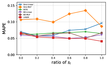
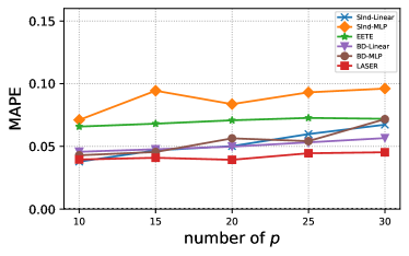
We generate two datasets to verify our method and theory. In the first dataset, we study the effect of the ratio of latent surrogates. Thus we fixed the number of observed short-term outcomes as and varied the ratio of latent surrogates. The range of numbers of variables in the first dataset are listed as follows: , and , where . The result is shown in Figure 5(a). In the second dataset, we study the effect of a varying number of proxies. Thus we do not generate and the numbers of are fixed as , and the range of numbers of proxies is: . The result is shown in Figure 5(b).
Sensitivity analysis of the ratio of latent surrogates. As shown in Figure 5(a), overall, LASER achieves the lowest MAPE. In detail, When the ratio of to is small, the traditional surrogacy assumption approximately holds and SInd-Linear, BD-Linear, BD-MLP, and EETE have similar performance to LASER. However, as the ratio of to increases, the performance of SInd-Linear, BD-Linear, BD-MLP and EETE becomes worse in different degrees. SInd-Linear gets worse most obviously, indicating it is not robust to the violation of the surrogacy assumption. SInd-MLP is unstable, and the reason may be the unmatched regression. LASER performs stable and effective, which means LASER is robust in different cases and verifies Corollary 5.5.
Sensitivity analysis of the number of proxies. As shown in Figure 5(b), LASER outperforms all baselines. In detail, as the number of noisy proxies increases, the MAPE of LASER stays below while other methods perform worse. The reason is that with the number of noisy proxies increasing, the noises, which bias the accuracy of causal effects estimation, increase too. The result shows that we can learn the latent surrogate representation well with the noisy proxies, whenever the number of proxies is small or large.
6.3 Additional Results of Semi-synthetic Dataset
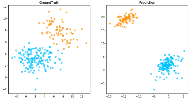
We further validate whether the iVAE-based LASER method can learn the latent surrogate representation as indicated by Theorem 5.3. Following the data generation in Section 6.2, we fixed the number of latent surrogates as 2, and fixed the number of observed surrogates as 0. The latent surrogates have two segments divided by the auxiliary treatment variables as shown in Figure 6. Then after applying our method, the recovered distribution (right) is very close to the true distribution (left) with some indeterminacy of scale which is reasonable due to the in our theoretical results. Therefore, we conclude that the latent surrogates can be identified by LASER.
7 Conclusions
In this paper, we provide a practical solution to the real-world problem of estimating long-term causal effects in the case that the surrogates are partially or even totally unobserved. Note that the observation of noisy proxies of the latent surrogates helps to learn a predictive representation for long-term causal effects estimation, even though the proxies and partially observed surrogates are mixed together and indistinguishable. Therefore, we propose an iVAE-based approach to learn a surrogate representation of the full short-term outcomes, without the need to distinguish the observed surrogates and proxies. Through such a unified view of the surrogates and the proxies of latent surrogates, we further devise an out-of-box, unbiased, and theoretically guaranteed solution to the long-term causal effects estimating problem. The extensive experiments, especially the real-world data experiments, validate the effectiveness of our method. A clear next step is to extend our work to robustly estimate long-term causal effects without the unconfoundedness assumption.
Acknowledgments
This research was supported in part by National Key R&D Program of China (2021ZD0111501), National Science Fund for Excellent Young Scholars (62122022), Natural Science Foundation of China (61876043, 61976052), the major key project of PCL (PCL2021A12).
References
- [1] H. Hohnhold, D. O’Brien, D. Tang, Focusing on the long-term: It’s good for users and business, in: Proceedings of the 21th ACM SIGKDD International Conference on Knowledge Discovery and Data Mining, 2015, pp. 1849–1858.
- [2] T. R. Fleming, R. L. Prentice, M. S. Pepe, D. Glidden, Surrogate and auxiliary endpoints in clinical trials, with potential applications in cancer and aids research, Statistics in medicine 13 (9) (1994) 955–968.
- [3] R. L. Prentice, Surrogate endpoints in clinical trials: definition and operational criteria, Statistics in medicine 8 (4) (1989) 431–440.
- [4] C. E. Frangakis, D. B. Rubin, Principal stratification in causal inference, Biometrics 58 (1) (2002) 21–29.
- [5] S. Athey, R. Chetty, G. W. Imbens, H. Kang, The surrogate index: Combining short-term proxies to estimate long-term treatment effects more rapidly and precisely, Tech. rep., National Bureau of Economic Research (2019).
- [6] L. Cheng, R. Guo, H. Liu, Long-term effect estimation with surrogate representation, in: Proceedings of the 14th ACM International Conference on Web Search and Data Mining, 2021, pp. 274–282.
- [7] N. Kallus, X. Mao, On the role of surrogates in the efficient estimation of treatment effects with limited outcome data, arXiv preprint arXiv:2003.12408 (2020).
- [8] J. Pearl, Causal inference in statistics: An overview, Statistics surveys 3 (2009) 96–146.
- [9] D. B. Rubin, Estimating causal effects of treatments in randomized and nonrandomized studies., Journal of educational Psychology 66 (5) (1974) 688.
- [10] P. R. Rosenbaum, D. B. Rubin, The central role of the propensity score in observational studies for causal effects, Biometrika 70 (1) (1983) 41–55.
- [11] P. R. Rosenbaum, Model-based direct adjustment, Journal of the American Statistical Association 82 (398) (1987) 387–394.
- [12] F. Johansson, U. Shalit, D. Sontag, Learning representations for counterfactual inference, in: International conference on machine learning, PMLR, 2016, pp. 3020–3029.
- [13] U. Shalit, F. D. Johansson, D. Sontag, Estimating individual treatment effect: generalization bounds and algorithms, in: International Conference on Machine Learning, PMLR, 2017, pp. 3076–3085.
- [14] C. Louizos, U. Shalit, J. M. Mooij, D. Sontag, R. S. Zemel, M. Welling, Causal effect inference with deep latent-variable models, in: NIPS, 2017.
- [15] W. Zhang, L. Liu, J. Li, Treatment effect estimation with disentangled latent factors, in: Proceedings of the AAAI Conference on Artificial Intelligence, Vol. 35, 2021, pp. 10923–10930.
- [16] C. Shi, V. Veitch, D. M. Blei, Invariant representation learning for treatment effect estimation, in: Uncertainty in Artificial Intelligence, PMLR, 2021, pp. 1546–1555.
- [17] S. Assaad, S. Zeng, C. Tao, S. Datta, N. Mehta, R. Henao, F. Li, L. C. Duke, Counterfactual representation learning with balancing weights, in: International Conference on Artificial Intelligence and Statistics, PMLR, 2021, pp. 1972–1980.
- [18] S. L. Lauritzen, O. O. Aalen, D. B. Rubin, E. Arjas, Discussion on causality [with reply], Scandinavian Journal of Statistics 31 (2) (2004) 189–201.
- [19] P. B. Gilbert, M. G. Hudgens, Evaluating candidate principal surrogate endpoints, Biometrics 64 (4) (2008) 1146–1154.
- [20] H. Chen, Z. Geng, J. Jia, Criteria for surrogate end points, Journal of the Royal Statistical Society: Series B (Statistical Methodology) 69 (5) (2007) 919–932.
- [21] C. Ju, Z. Geng, Criteria for surrogate end points based on causal distributions, Journal of the Royal Statistical Society: Series B (Statistical Methodology) 72 (1) (2010) 129–142.
- [22] Y. Yin, L. Liu, Z. Geng, P. Luo, Novel criteria to exclude the surrogate paradox and their optimalities, Scandinavian Journal of Statistics 47 (1) (2020) 84–103.
- [23] S. Athey, R. Chetty, G. Imbens, Combining experimental and observational data to estimate treatment effects on long term outcomes, arXiv preprint arXiv:2006.09676 (2020).
- [24] G. Imbens, N. Kallus, X. Mao, Y. Wang, Long-term causal inference under persistent confounding via data combination, arXiv preprint arXiv:2202.07234 (2022).
-
[25]
D. P. Kingma, M. Welling, Auto-encoding
variational bayes, in: Y. Bengio, Y. LeCun (Eds.), 2nd International
Conference on Learning Representations, ICLR 2014, Banff, AB, Canada, April
14-16, 2014, Conference Track Proceedings, 2014.
URL http://arxiv.org/abs/1312.6114 - [26] D. J. Rezende, S. Mohamed, D. Wierstra, Stochastic backpropagation and approximate inference in deep generative models, in: International conference on machine learning, PMLR, 2014, pp. 1278–1286.
- [27] I. Higgins, L. Matthey, A. Pal, C. Burgess, X. Glorot, M. Botvinick, S. Mohamed, A. Lerchner, beta-vae: Learning basic visual concepts with a constrained variational framework (2016).
- [28] R. Lopez, J. Regier, M. I. Jordan, N. Yosef, Information constraints on auto-encoding variational bayes, in: NeurIPS, 2018.
-
[29]
O. Rybkin, K. Daniilidis, S. Levine,
Simple and effective
vae training with calibrated decoders, in: M. Meila, T. Zhang (Eds.),
Proceedings of the 38th International Conference on Machine Learning, Vol.
139 of Proceedings of Machine Learning Research, PMLR, 2021, pp. 9179–9189.
URL https://proceedings.mlr.press/v139/rybkin21a.html -
[30]
Q. Wang, T. P. Breckon,
Generalized
zero-shot domain adaptation via coupled conditional variational
autoencoders, Neural Networks (2023).
doi:https://doi.org/10.1016/j.neunet.2023.03.033.
URL https://www.sciencedirect.com/science/article/pii/S0893608023001697 - [31] I. Khemakhem, D. Kingma, R. Monti, A. Hyvarinen, Variational autoencoders and nonlinear ica: A unifying framework, in: International Conference on Artificial Intelligence and Statistics, PMLR, 2020, pp. 2207–2217.
- [32] W. Yao, Y. Sun, A. Ho, C. Sun, K. Zhang, Learning temporally causal latent processes from general temporal data, arXiv preprint arXiv:2110.05428 (2021).
- [33] J. Pearl, Causality, Cambridge university press, 2009.
- [34] J. L. Hill, Bayesian nonparametric modeling for causal inference, Journal of Computational and Graphical Statistics 20 (1) (2011) 217–240.
- [35] J. Pearl, [bayesian analysis in expert systems]: comment: graphical models, causality and intervention, Statistical Science 8 (3) (1993) 266–269.
Appendix A Proof of Theorem 5.3
We now prove Theorem 5.3 that under mild assumptions, we can recover the latent up to some simper transformations. The proof is based on the proof of Theorem 1 in Khemakhem et al. [31], with the following differences:
-
1.
We use both and as auxiliary variables, and treat and as latent variables;
-
2.
We consider different causal mechanism of generating observed variables .
Proof.
Suppose we have two sets of parameters and such that , then:
| (1) | ||||
In Eq. 1, we denote the volume of a matrix as . denotes the Jacobian. We made the change of variable on the left-hand side and on the right-hand side.
In determining function , i.e., , the term in Eq.1 can be written as and then is vanished. Thus, we have the following equation:
| (2) |
By taking the logarithm on both side of Eq. 2 and replacing by its expression from Eq. 9 under Assumption 5.1, we have:
| (3) | ||||
Let distinct points be the point provided by the condition (2) of Theorem, and define . We evaluate the above equations at these points to obtain equations, and subtract the first equation from the remaining equations to obtain, for :
| (4) | ||||
Let be the matrix defined in condition (2) and similarly defined for (note that is not necessarily invertible). Define and the vector of all for .
Then Eq.4 can be rewritten in the matrix form:
Then we multiply both sides of the above equation by to get:
| (5) |
where and .
We next show that is invertible. By definition of and according to condition (1), its Jacobian exists and is a matrix of rank . This implies that the Jacobian of exists and is of rank and so is .
If , is invertible because is matrix of rank .
If , is also invertible because:
Define and .
First, we prove, by contradiction, that for each , there exist k points such that for the distribution the family are linearly independent. Suppose for any choice of , the family is never linearly independent. This means that is included in a subspace of of the dimension of most . Let be a non-zero vector that is orthogonal to . Then for all , we have . By integrating we find that . Since this is true for all and a , we conclude that the distribution is not strongly exponential, which contradicts the definition of distribution of . So by contradiction, we conclude that there exist k points such that are linearly independent.
Second, we prove the invertibility of . Collect these points to vectors and concatenate the Jacobians evaluated at each of those vectors horizontally into the matrix and similarly define as the concatenation of Jacobians of evaluated at those points. Then the matrix is invertible. By differentiating Eq. 5 for each , we have:
The invertibility of implies the invertibility of and , which completes the proof. ∎
Appendix B Proof of Theorem 5.4.
Proof.
The IPW method allows us to estimate causal effects by
| (6) | ||||
For simplicity, we only discuss the case of . We define the unbiased long-term outcome predictor , and in practice the predictor that we use is . We bridge the two predictors as follows:
| (7) | ||||
where the fourth equation holds due to , and the fifth equation holds due to the invertibility of .
Hence, the long-term causal effects are identifiable. ∎
Appendix C Proof of Corollary 5.5.
Proof.
As shown in Figure 4, this two cases are special cases of our generalized causal graph in Figure 2(b), and we discuss respectively:
Special case 1: in this case, we observe the whole valid surrogates. We can consider this case as that we observe noiseless proxies with the latent surrogates: and also , which means the defined in Eq. 7 is in a linear form with coefficient , i.e., . Thus the parameters is still when Theorem 5.3 hold. In such a case we can still recover . Thus, suppose Theorem 5.4 holds, the causal effects are also identifiable.
Special case 2: in this case, we only observe the proxies of surrogates. Without observing one of the surrogates, we consider and , which develops into the standard latent identification problem as discussed in Khemakhem et al. [31]. Thus the parameters is when Theorem 5.3 holds and then the causal effects are also identifiable when Theorem 5.4 holds. ∎
Appendix D ELBO Derivation
Our object function contains and a extra loss minimizing predicting error of long-term outcome . We give the derivation as follows:
| (8) | ||||
where is the empirical data distribution given by dataset .
Appendix E Additional Experiments
| Subject | Property | : Number | Exist In | |
| dimension | : 123 | |||
| (all surrogates) | dimension | : 122 | ||
| (revenues only) | dimension | : 7 | ||
| dimension | : 1 | |||
| sample size of observational data | Strategy1 | sample size | : 34866 | |
| Strategy2 | sample size | : 34992 | ||
| Strategy3 | sample size | : 35010 | ||
| Strategy4 | sample size | : 34929 | ||
| Strategy5 | sample size | : 35010 | ||
| Strategy6 | sample size | : 34893 | ||
| Strategy7 | sample size | : 34920 | ||
| Strategy8 | sample size | : 35046 | ||
| sample size of experimental data | Strategy1 | sample size | : 3874 | |
| Strategy2 | sample size | : 3888 | ||
| Strategy3 | sample size | : 3890 | ||
| Strategy4 | sample size | : 3881 | ||
| Strategy5 | sample size | : 3890 | ||
| Strategy6 | sample size | : 3877 | ||
| Strategy7 | sample size | : 3880 | ||
| Strategy8 | sample size | : 3894 |
E.1 Additional Real-world Dataset
To further validate the effectiveness of LASER, we conduct additional experiments on another much larger real-world dataset than the dataset in Section 6.1. The dataset is collected from an online randomized controlled experiment on the Chinese largest ride-hailing platform, aiming to measure the effects of 9 different campaign strategies across 30 cities for 14 days. We record the first 7 days’ user behavior as surrogates and the 14th day cumulative revenue as the long-term outcome. We compare LASER with baseline methods on 8 different campaign strategies. The detailed information of this real-world dataset is listed in Table 4. The detailed results on this dataset are listed in Table 5 and Table 6. The results are similar to the results in Section 6.1, strengthening our experimental conclusions. Moreover, LASER still performs well in the larger dataset, showing its robustness in the high dimensional case.
| LASER | LASER-GRU | SInd-Linear | SInd-MLP | LTEE | EETE | BD-Linear | BD-MLP | |
|---|---|---|---|---|---|---|---|---|
| Strategy | mean | mean | mean | mean | mean | mean | mean | mean |
| Strategy1 | 0.0296 | 0.0660 | 0.2787 | 0.2597 | 0.1247 | 0.1668 | 0.3060 | 0.4028 |
| Strategy2 | 0.0132 | 0.0066 | 0.1867 | 0.1931 | 0.0388 | 0.1825 | 0.2523 | 0.3163 |
| Strategy3 | 0.0047 | 0.0086 | 0.1987 | 0.1906 | 0.0281 | 0.1399 | 0.2415 | 0.1511 |
| Strategy4 | 0.0047 | 0.0578 | 0.2032 | 0.1974 | 0.0151 | 0.0517 | 0.2370 | 0.1947 |
| Strategy5 | 0.0039 | 0.0056 | 0.1617 | 0.1620 | 0.0092 | 0.0442 | 0.2266 | 0.1986 |
| Strategy6 | 0.1137 | 0.1076 | 0.1571 | 0.1838 | 0.1202 | 0.1840 | 0.2152 | 0.2583 |
| Strategy7 | 0.0639 | 0.0814 | 0.1078 | 0.1193 | 0.1435 | 0.1163 | 0.2057 | 0.1562 |
| Strategy8 | 0.0530 | 0.0253 | 0.1578 | 0.1691 | 0.0674 | 0.2081 | 0.2168 | 0.1871 |
| Average | 0.0358 | 0.0449 | 0.1815 | 0.1844 | 0.0684 | 0.1367 | 0.2376 | 0.2331 |
| LASER | LASER-GRU | SInd-Linear | SInd-MLP | LTEE | EETE | BD-Linear | BD-MLP | |
|---|---|---|---|---|---|---|---|---|
| Strategy | mean | mean | mean | mean | mean | mean | mean | mean |
| Strategy1 | 0.0822 | 0.1120 | 0.3067 | 0.2906 | 0.1059 | 0.1653 | 0.2783 | 0.2148 |
| Strategy2 | 0.0042 | 0.0480 | 0.1993 | 0.2058 | 0.0321 | 0.1827 | 0.2322 | 0.1616 |
| Strategy3 | 0.0272 | 0.0467 | 0.2198 | 0.2255 | 0.0288 | 0.1390 | 0.2211 | 0.1851 |
| Strategy4 | 0.0083 | 0.0123 | 0.2235 | 0.2310 | 0.0157 | 0.0515 | 0.2166 | 0.1964 |
| Strategy5 | 0.0043 | 0.0066 | 0.1851 | 0.1941 | 0.0096 | 0.0444 | 0.2057 | 0.1518 |
| Strategy6 | 0.0947 | 0.0986 | 0.1711 | 0.2188 | 0.1433 | 0.1853 | 0.1997 | 0.2254 |
| Strategy7 | 0.0157 | 0.0206 | 0.1489 | 0.1322 | 0.1377 | 0.1194 | 0.1865 | 0.1706 |
| Strategy8 | 0.0314 | 0.0146 | 0.2952 | 0.2656 | 0.0603 | 0.2072 | 0.1828 | 0.1400 |
| Average | 0.0335 | 0.0449 | 0.2187 | 0.2205 | 0.0667 | 0.1369 | 0.2153 | 0.1807 |