OptEmbed: Learning Optimal Embedding Table for Click-through Rate Prediction
Abstract.
Click-through rate (CTR) prediction model usually consists of three components: embedding table, feature interaction layer, and classifier. Learning embedding table plays a fundamental role in CTR prediction from the view of the model performance and memory usage. The embedding table is a two-dimensional tensor, with its axes indicating the number of feature values and the embedding dimension, respectively. To learn an efficient and effective embedding table, recent works either assign various embedding dimensions for feature fields and reduce the number of embeddings respectively or mask the embedding table parameters. However, all these existing works cannot get an optimal embedding table. On the one hand, various embedding dimensions still require a large amount of memory due to the vast number of features in the dataset. On the other hand, decreasing the number of embeddings usually suffers from performance degradation, which is intolerable in CTR prediction. Finally, pruning embedding parameters will lead to a sparse embedding table, which is hard to be deployed. To this end, we propose an optimal embedding table learning framework OptEmbed, which provides a practical and general method to find an optimal embedding table for various base CTR models. Specifically, we propose pruning the redundant embeddings regarding corresponding features’ importance by learnable pruning thresholds. Furthermore, we consider assigning various embedding dimensions as one single candidate architecture. To efficiently search the optimal embedding dimensions, we design a uniform embedding dimension sampling scheme to equally train all candidate architectures, meaning architecture-related parameters and learnable thresholds are trained simultaneously in one supernet. We then propose an evolution search method based on the supernet to find the optimal embedding dimensions for each field. Experiments on public datasets show that OptEmbed can learn a compact embedding table which can further improve the model performance.
1. Introduction
Click-through rate (CTR) prediction has been a critical task in real-world commercial recommender systems and online advertising systems (Chapelle et al., 2015; Naumov et al., 2019). It aims to predict the probability of a certain user clicking a recommended item (e.g. movie, advertisement) (Rendle, 2010; Guo et al., 2017; Wang et al., 2017; Song et al., 2019). General CTR prediction model architecture consists of embedding table, interaction layer, and classifier as illustrated in Fig. 1 (Wei et al., 2021; Guo et al., 2017; Wang et al., 2017; Song et al., 2019). The typical inputs of CTR models consist of many categorical features. We term the values of these categorical features as feature values, which are organized as feature fields. For example, a feature field gender contains three feature values, male, female and unknown. These predictive models use the embedding table to map the categorical feature values into real-valued dense vectors. Then these embeddings are fed into the feature interaction layer, such as factorization machine (Rendle, 2010), cross network (Wang et al., 2017), self-attention layer (Song et al., 2019). The final classifier aggregates the representation vector to make the prediction.
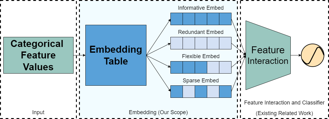
In the general CTR prediction model architecture, the embedding table dominates the number of parameters and plays a fundamental role in prediction performance. Therefore, it is critical to obtain optimal embedding tables that reduce the model size and improve performance (Kang et al., 2020; Shi et al., 2020). The embedding table is a two-dimensional tensor , which maps each feature value to an indexed row. The first dimension size thus equals the total number of feature values, and the second one is the embedding dimension. The memory cost of the embedding table is , where mainly decides the memory usage given . When all possible feature values are fed into the model (Guo et al., 2017; He and Chua, 2017), becomes a vast number (up to millions on web-scale applications). This leads to a large number of embeddings, which contributes to the primary memory bottleneck within both training and inference (Guo et al., 2021). However, the redundant embedding not only necessitates additional memory cost but is also detrimental to the model performance (Wang et al., 2022). Therefore, the first requirement for an optimal embedding table is to distinguish the redundant embeddings and zero them out before they are fed into the following layers, as shown in Fig. 1. The embedding dimension is mostly fixed across all the feature values. Previous works(Kang et al., 2020; Zhao et al., 2021) point out that the over-parameterizing features with smaller feature cardinality may induce overfitting, and features with larger cardinality need larger dimensions to convey fruitful information. Hence, the second requirement for an optimal embedding table is to assign various embedding dimensions to feature values as flexible embedding shown in Fig. 1. An alternative to optimize the embedding table is to mask the embedding parameters directly (Qu et al., 2022; Liu et al., 2021). It makes embedding dimension with discontinuous parameters, illustrated as sparse embedding in Fig. 1. Nevertheless, the sparse embedding table requires storing extra structural information and additional computation cost in the inference stage, which is not suitable for hardware in practical (Deng et al., 2021). The final requirement is to optimize the embedding table without storing additional structural information on hardware requirements. Given the above requirements, it is highly desired to prune redundant embeddings and search embedding dimensions in a unifying way.
Previous work on optimizing the embedding table either treats embedding reduction and dimensions search separately or generates sparse embedding. To reduce the number of embeddings, one natural approach is to design a hash function, which maps the categorical features to the embedding table index (Weinberger et al., 2009; Zhang et al., 2020; Yan et al., 2021a). Since the embedding table index size is far less than the number of feature values, this approach optimizes memory usage. However, blindly mapping different feature values into the same embeddings without distinguishing the redundant embeddings may lead to performance degradation, which is intolerable in CTR prediction. On the other hand, AutoField (Wang et al., 2022) utilizes the differential architecture search (Liu et al., 2019) method to prune redundant feature fields. But this method may prune some informative feature values while preserving some redundant ones since the feature field is not fine-grained enough to generate an optimal embedding. To search for flexible embedding dimension, AutoDim (Zhao et al., 2021) also utilize the differential architecture search (Liu et al., 2019) method. However, this method cannot get an optimal embedding table, as it does not remove redundant features. Moreover, some research optimizes the embedding table in a unifying way based on embedding pruning (Liu et al., 2021; Shen et al., 2021; Qu et al., 2022). These methods identify and mask redundant values in embeddings, where embeddings are pruned when their dimensions are equal to zero. However, these methods result in a sparse embedding table, which poses challenges when fitting into modern computation units.
In this paper, we propose a framework to address two main challenges and learn an optimal embedding table (OptEmbed) that satisfy all three requirements. First, for the problem of how to prune the redundant embeddings and search feature fields embedding dimensions in a unifying way, we transform it into the problem of identifying the importance of each feature value. Besides, searching field-wise embedding dimensions can be formulated as an architecture search problem. To this end, inspired by structural pruning and network architecture search (Frankle and Carbin, 2019; Cai et al., 2019), we introduce learnable pruning thresholds to distinguish informative embeddings and to allocate the dimensions to those embeddings in an automated and data-driven manner. Specifically, we mask redundant embeddings adaptively with thresholds. Meanwhile, we design a uniform embedding dimension sampling scheme to train a supernet with the learnable thresholds. Then, We conduct an evolutionary search based on the supernet with informative embeddings to assign optimal field-wise dimensions. To address the second challenge of how to optimize the embedding table efficiently, we reparameterize the problem with a threshold vector, which makes the original problem differentiable and only needs a few preallocate memory (Donà and Gallinari, 2021). Moreover, the search space of embedding dimensions is also too huge to explore (Zhao et al., 2021). Therefore, we design a one-shot embedding dimension search method to save search time by decoupling parameter training and dimension search based on the supernet mentioned above. The experimental results on three public datasets demonstrate the efficiency and effectiveness of our proposed framework OptEmbed. We summarize our major contributions as below:
-
•
This paper firstly proposes the requirements for an optimal embedding table: no redundant embedding, embedding dimension flexible and hardware friendly. We propose a novel optimization method called OptEmbed, which improves model performance and reduces memory usage based on these requirements.
-
•
The proposed OptEmbed optimizes the embedding table in a unifying way. It can efficiently train a supernet with informative feature values and the embedding parameters simultaneously. Moreover, we design a one-shot embedding dimension search method based on the supernet, which produces the optimal embedding table without sparse embedding.
-
•
The extensive experiments are conducted on three public datasets. The experimental results demonstrate the effectiveness and efficiency of the proposed framework.
We organize the rest of this paper as follows. In Section 2, we formulate the CTR prediction problem and three requirements for the optimal embedding table. In Section 3, we present OptEmbed to obtain the optimal embedding table efficiently. Section 4 details the experiments. In Section 5, we briefly introduce related works. Finally, we conclude this work in Section 6.
2. Problem Definition
In this section, we formulate how the CTR prediction model output the prediction result with the concatenation of multiple features and define the requirements for an optimal embedding table.
2.1. CTR Prediction
We represent the raw inputs as the raw feature vector that concatenates feature fields . Usually, is a one-hot representation, which is very sparse and high-dimensional. For example, the feature field gender has three unique feature values, male,female, and unknown, then they can be represented by three one-hot vectors , and , respectively. Before raw feature vectors are fed into the feature interaction layer, we usually employ embedding table to convert them into low dimensional and dense real-value vectors. This can be formulated as , where is the embedding table, is the number of feature values and is the size of embedding. Then embeddings are stacked together as a embedding vector .
Following learnable embedding table, the feature interaction layer will be performed based on in mainstream CTR models. There are several types of feature interaction in previous study, e.g. inner product (Guo et al., 2017). As discussed in previous work (Meng et al., 2021), feature interaction can be defined as based on embeddings:
| (1) |
where can be a single layer perceptron or cross layer(Wang et al., 2017). The feature interaction can be aggregated together:
| (2) |
where symbol denotes the concatenation operation, is the output of feature interaction, and is network parameters except for embedding table. The cross entropy loss (i.e. log-loss) is adopted for training the model:
| (3) |
We summarize the final CTR prediction problem as follows:
| (4) |
where is the ground truth of user clicks, is the training dataset.
2.2. Optimal Embedding Table
The original embedding table is neither effective nor efficient (Zhao et al., 2021; Wang et al., 2022; Wei et al., 2021; Liu et al., 2021). An optimal embedding table that satisfies the following requirements can greatly reduce the model size and improve performance:
Req. 1.
No Redundant Embeddings: The optimal embedding table should only map informative feature values to embeddings. Feature value is considered informative if the performance of the model is degraded when masking its corresponding embedding . Otherwise, it is deemed to be redundant.
Req. 2.
Embedding Dimension Flexible: The optimal embedding table should assign various embedding dimensions, improving the performance of the predictive model the most.
Req. 3.
Hardware Friendly: The optimal embedding table should be compatible with the modern parallel-processing hardware (e.g. GPU) – requiring no additional resources when training and inference.
To fulfill the three requirements above, we decompose the original single embedding table into a series of field-wise embedding tables , where . To satisfy requirement (i), we prune some embeddings related to redundant feature values, which can be formulated as . As to requirements (ii) and (iii), different embedding sizes for each field-wise embedding tables are allocated. In summary, an optimal embedding table can be further defined as:
| (5) | ||||
Notes that previous methods can not satisfy all three requirements. We will detail this in Section 3.4.
3. OptEmbed
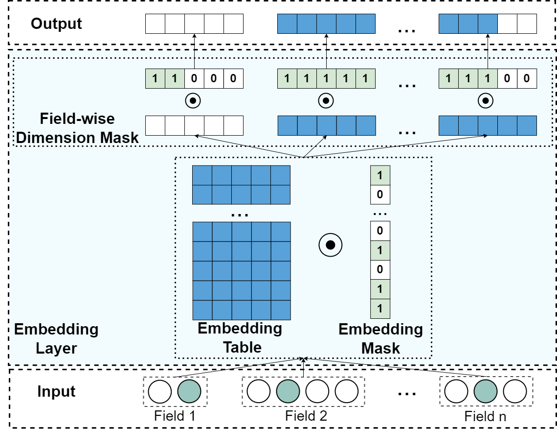
In this section, we propose a framework called OptEmbed to learn the optimal embedding table defined in Section 2. We rewrite Eq. 5 into the following by introducing two masks:
| (6) |
Here denotes the field-wise dimension mask. denotes the embedding mask. and denote the feature number and field number. denotes element-wise product with broadcasting. By doing so, we decompose the task of learning the optimal embedding table into three parts: (i) train embedding mask to preserve informative embeddings; (ii) search for field-wise dimension mask to assign various embedding size to each field and (iii) re-train the optimal embedding table under the constraints of (i) and (ii). The overview of OptEmbed framework is shown in Fig. 2. Both the embedding mask and dimension mask are applied to the embedding table. Some of the embeddings are removed, while others become sparse.
Below, we first illustrate how to determine embedding mask and field-wise dimension mask , respectively. We then introduce the re-training stage and discuss how OptEmbed compares with other methods that optimize the architecture of embedding tables from various aspects.
3.1. Redundant Embedding Pruning
The redundant embedding pruning component determines which rows of the embedding table are informative and should be included in the final prediction task. Given that tends to be a large number, it is computationally inefficient to assign individual parameters to each feature marking its importance. Inspired by network pruning (Liu et al., 2020a; Yuan et al., 2021), we directly optimize the embedding table and adaptively pruning the embeddings via comparing with field-wise threshold, which can be updated by gradient descent. The reparameterization of the is formulated as follows:
| (7) |
where is the field-wise threshold vector, is the norm of embedding in each field, is the activation function, which works as trainable dynamic mask. We will illustrate three parts in the following sections in details.
3.1.1. Field-wise Threshold Vector
We introduce a trainable field-wise vector to serve as pruning thresholds for embeddings in every field. We do not adopt a global threshold because corresponding features from different fields are likely to have different properties. For instance, the average frequency for the gender field is expected to be much higher than that for the ID field. Assessing the importance of features from different fields with a global threshold value would lead to a non-robust and hard-to-train network. Meanwhile, we do not adopt a feature-wise threshold vector considering it would significantly increase the number of total parameters and make it more likely to over-fit.
3.1.2. norm
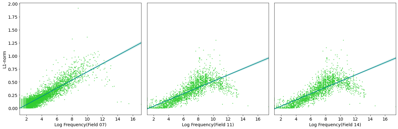
It is commonly believed that features with higher frequency tend to be more important and informative in CTR prediction (Yan et al., 2021b; Zhang et al., 2020). To measure the importance of features precisely, we empirically train a prediction model and investigate the relation between the frequency of each feature and norm of the corresponding embedding in each field. Three fields in Avazu dataset111http://www.kaggle.com/c/avazu-ctr-prediction are randomly selected as an example; here we set the base model as FNN (Zhang et al., 2016), norm as norm. The results are illustrated in Fig. 3. Each green dot represents one embedding in the embedding table, with its x-axis denoting the norm of the embedding and y-axis denoting the log frequency of the corresponding feature value. A fitting curve is also shown in blue to summarize the relationships between these two variables. As we can observe, with the increment of feature frequency, the norm of the corresponding embedding also grows linearly. As a result, we adopt norm of corresponding embeddings as a measurement in our framework (Liu et al., 2020a; Han et al., 2015).
3.1.3. Unit Step Function
We introduce a unit step function as the activation function to generate a binary mask. Given the field-wise threshold vector and unit step function , we can formally generate the embedding mask . For feature corresponding embedding , its embedding mask is given by:
| (8) |
where indicates the normalization function and maps feature to the corresponding field. With the unit step function , we can easily generate binary embedding mask . Then the embedding table can be formulated as
| (9) |
The prediction score will be calculated with . However, because the derivative of step unit function is an impulse function, Eq.9 cannot be directly optimized. To preserve gradients and make the model trainable, we adopt the long-tail derivation estimator (Liu et al., 2020a) to replace the gradient of the step unit function. The long-tail derivation estimator can be formulated as
| (10) |
We adopt this derivative long-tail estimator to optimize the field-wise threshold vector , so that the gradient would be large when the norm and the threshold value are close to each other and would be 0 when the gap between norm and threshold value are large enough. We denote the gradient of actual embedding as . Notes that the gradient of embedding for updating is
| (11) |
The gradient of embedding is composed of two parts. The first part is the performance gradient that improves the performance. The second part is the structure gradient that removes redundant embeddings. As the final embedding is jointly influenced by both the performance and structure, OptEmbed can recover some embeddings. Specifically, once an embedding is accidentally removed, the performance gradient becomes zero because the embedding is zeroed-out. However, the embedding still receives the structure gradient. So the pruned embedding may be recovered again if the gap between norm and threshold are not too large (i.e. smaller than one in this case).
It is worth mentioning that the in norm needs to be carefully selected. With for embedding , we can get derivation for particular element:
| (12) |
Due to the first term , the gradient of will be influenced by all elements from embedding unless . Therefore we select for OptEmbed hereafter to get rid of the influence.
3.1.4. Sparse Regularization Term
To remove more redundant embeddings, higher thresholds are encouraged. To achieve this, we explicitly add an exponential regularization term to the logloss that penalizes low threshold values. For the field-wise threshold , the exponential regularization term is
| (13) |
Notice that the regularization term gradually decreases to zero as increases. Hence, the final objective in this stage becomes
| (14) |
Here is the scaling coefficient for the sparse regularization term, controlling how many embeddings are pruned. With higher , tends to increase the threshold , which makes it easier to prune redundant embeddings. However, once becomes too large, it may accidentally remove certain informative embeddings, leading to the increase of the cross-entropy loss . Therefore, our method can dynamically remove redundant embeddings, leading to a proper balance between model performance and size.
3.2. Embedding Dimension Search
The embedding dimension search component aims to assign various optimal dimensions for all fields. By viewing a group of field-wise dimension masks as one neural network architecture, we design an efficient neural architecture search method to search for optimal dimension masks efficiently in this section.
3.2.1. One-shot NAS Problem
Because the optimal embedding table should satisfy Req. 2 and 3, the dimensionality set in our method, formed by all candidate embedding dimensions, can be formulated as . Notice that the complexity of this search space is , which is impossible to search all the possible architectures in the search space exhaustively. On the other hand, to evaluate architecture, we need to train and network parameters again, which costs a lot of computation resources. To efficiently search for the optimal embedding dimension mask, we hence re-formulate the dimension search as a one-shot NAS problem (Guo et al., 2020; Bender et al., 2018):
| (15) | ||||
where denotes the search space, is the prior distribution of the search space, is the best supernet parameter and denotes the parameter space of the supernet. By decoupling the dependency between training embedding and dimension search, we no longer need to train a sub-architecture from scratch, which reduces computation cost significantly.
3.2.2. Supernet Training
Following Eq. 15, we construct the supernet embedding table with ordinal parameter sharing (Wei et al., 2021), which is efficient to reuse most of parameters. In our method with search space , the supernet is constructed with maximum dimension . With no prior knowledge of , we then assume as a uniform distribution. Such an assumption proves to be empirically good enough and efficient to apply (Guo et al., 2020). Specially, given , the first elements of are ones and the rest are zeros. Different from other methods (Liu et al., 2021; Qu et al., 2022), induce flexible embedding, which is hardware-friendly, instead of sparse embedding, which requires a lot of structure information.
Moreover, the retains various embeddings during training both and embedding parameters, which affects the supernet directly. To train the supernet adapting to and reduce the total training time further, we conduct the supernet training and redundant embedding pruning in a unifying way by introducing . Finally, we can formulate supernet training as:
| (16) | ||||
3.2.3. Search Strategy
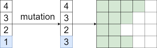
After training the supernet from Eq. 16, we present an evolutionary search for the optimal dimension mask . In the beginning, all candidates are randomly generated. At every epoch, each candidate dimension mask is evaluated on the validation set by inheriting parameters from the supernet. This part is relatively efficient as no training is involved. After the evaluation, the Top-k candidates are preserved for crossover and mutation operation to generate the candidates for the next epoch. For crossover, two randomly selected candidates are crossed to produce a new one by selecting a random point where the parents’ parts exchange happens. Fig. 4(b) details an example where the blue parts of the two candidates are crossed. For mutation, a randomly selected candidate mutates its choice at each position with the given mutation probability . An example is illustrated in Fig. 4(a) where the blue point is a random mutation. Crossover and mutation are repeated to generate enough new candidates given the corresponding number and . After epoch, we output the best-performed candidate dimension mask as the optimal dimension mask . This process is shown in Algorithm 1 in line 7-17.

3.3. Parameter Re-training
During the supernet training, we map all raw features into embeddings. Thus to eliminate the influence of these embeddings, a re-training stage is desired to train the model with only optimal number of embeddings and embedding dimensions. The embedding mask and the field-wise dimension mask are obtained followed Eq. 16. In the re-training stage, the objective becomes
| (17) |
In summary, the overall process of OptEmbed can be summarized as Algorithm 1.
3.4. Method Discussion
The combination of pruning redundant embeddings and embedding dimension search makes our OptEmbed approach efficient and effective. Table 1 performs a comprehensive comparison of our approach with others that optimize embedding table on whether they satisfied the Req. 1, 2 and 3. Some methods (Ginart et al., 2021; Cheng et al., 2020; Zhao et al., 2021; Wei et al., 2021; Kang et al., 2020) search optimal dimension for embedding table from different granularity: feature-wise (usually grouped by feature value frequency) or field-wise. Another method (Shi et al., 2020) uses hashing technique to reduce the number of embeddings in the embedding table. The other methods (Shen et al., 2021; Liu et al., 2021) utilize pruning techniques (Liu et al., 2020a; Frankle and Carbin, 2019) to learn the sparse embedding table directly, which is hard to compatible with the hardware. OptEmbed method is the only method that satisfies Req. 1, 2 and 3. The rest of the method tends to violate one or two requirements.
| Approach | R1: N.R.F. | R2: E.D.F. | R3: H.F. |
|---|---|---|---|
| MDE (Ginart et al., 2021) | ✗ | ✓ | ✓ |
| DNIS (Cheng et al., 2020) | ✗ | ✓ | ✓ |
| AutoDim (Zhao et al., 2021) | ✗ | ✓ | ✓ |
| AutoField (Wang et al., 2022) | ✓ | ✗ | ✓ |
| QR (Shi et al., 2020) | ✓ | ✗ | ✓ |
| PEP (Liu et al., 2021) | ✓ | ✓ | ✗ |
| OptEmbed | ✓ | ✓ | ✓ |
-
1
N.R.F, E.D.F. and H.F. are abbreviations for No Redundant Feature, Embedding Dimension Flexible and Hardwar Friendly.
4. experiment
We design experiments to answer the following research questions:
-
•
RQ1: Could OptEmbed achieve superior performance compared with mainstream CTR prediction models and other algorithms that optimize the embedding table?
-
•
RQ2: How does each component of OptEmbed contribute to the final result?
-
•
RQ3: What is the impact of the re-training stage in OptEmbed on the final result?
-
•
RQ4: How efficient is OptEmbed compared with SOTA handcrafted models and other algorithms that optimize the embedding table?
-
•
RQ5: Does OptEmbed output the optimal embedding table?
4.1. Experiment Setup
4.1.1. Datasets
We conduct our experiments on three public datasets. In all following dataset, we randomly split them into as the training set, validation set, and test set respectively.
Criteo222https://www.kaggle.com/c/criteo-display-ad-challenge dataset consists of ad click data over a week. It consists of 26 categorical feature fields and 13 numerical feature fields. We follow the winner solution of the Criteo contest to discretize each numeric value to , if ; otherwise. Following the best practice (Zhu et al., 2021), we replace infrequent categorical features with a default ”OOV” (i.e. out-of-vocabulary) token, with min_count=2.
Avazu333http://www.kaggle.com/c/avazu-ctr-prediction dataset contains 10 days of click logs. It has 24 fields with categorical features, including instance id, app id, device id, etc. Following the best practice (Zhu et al., 2021), we remove the instance id field and transform the timestamp field into three new fields: hour, weekday and is_weekend. We replace infrequent categorical features with the ”OOV” token, with min_count=2.
KDD12444http://www.kddcup2012.org/c/kddcup2012-track2/data dataset contains training instances derived from search session logs. It has 11 categorical fields, and the click field is the number of times the user clicks the ad. We replace infrequent features with an ”OOV” token, with min_count=10.
| Dataset | DeepFM | DCN | FNN | IPNN | |||||||||
|---|---|---|---|---|---|---|---|---|---|---|---|---|---|
| AUC | Logloss | Sparsity | AUC | Logloss | Sparsity | AUC | Logloss | Sparsity | AUC | Logloss | Sparsity | ||
| Criteo | Original | 0.8104 | 0.4409 | - | 0.8106 | 0.4408 | - | 0.8110 | 0.4404 | - | 0.8113 | 0.4401 | - |
| AutoDim | 0.8093 | 0.4420 | 0.8642 | 0.8096 | 0.4418 | 0.7917 | 0.8104 | 0.4410 | 0.7187 | 0.8103 | 0.4411 | 0.7179 | |
| AutoField | 0.8101 | 0.4412 | 0.0009 | 0.8108 | 0.4405 | 0.4108 | 0.8108 | 0.4406 | 0.6221 | 0.8111 | 0.4403 | 0.3941 | |
| QR | 0.8084 | 0.4444 | 0.5000 | 0.8103 | 0.4411 | 0.5000 | 0.8105 | 0.4408 | 0.5000 | 0.8102 | 0.4411 | 0.5000 | |
| PEP | 0.7980 | 0.4541 | 0.5010 | 0.8110 | 0.4404 | 0.5802 | 0.8108 | 0.4406 | 0.5802 | 0.8111 | 0.4402 | 0.5607 | |
| OptEmbed | 0.8105 | 0.4409 | 0.9684 | 0.8113 | 0.4402 | 0.8534 | 0.8114 | 0.4400 | 0.6710 | 0.8114 | 0.4401 | 0.7122 | |
| Avazu | Original | 0.7884 | 0.3751 | - | 0.7894 | 0.3748 | - | 0.7896 | 0.3748 | - | 0.7898 | 0.3745 | - |
| AutoDim | 0.7843 | 0.3779 | 0.6936 | 0.7893 | 0.3744 | 0.5013 | 0.7894 | 0.3743 | 0.5017 | 0.7894 | 0.3743 | 0.3892 | |
| AutoField | 0.7866 | 0.3762 | 0.0020 | 0.7887 | 0.3748 | 0.0001 | 0.7892 | 0.3748 | 0.0001 | 0.7897 | 0.3744 | 0.0001 | |
| QR | 0.7762 | 0.3821 | 0.5000 | 0.7868 | 0.3766 | 0.5000 | 0.7857 | 0.3769 | 0.5000 | 0.7849 | 0.3781 | 0.5000 | |
| PEP | 0.7877 | 0.3754 | 0.4126 | 0.7896 | 0.3743 | 0.3016 | 0.7894 | 0.3744 | 0.3016 | 0.7897 | 0.3742 | 0.3016 | |
| OptEmbed | 0.3740 | 0.6840 | 0.3744 | 0.5563 | 0.7902 | 0.4693 | |||||||
| KDD12 | Original | 0.7962 | 0.1532 | - | 0.8010 | 0.1522 | - | 0.8008 | 0.1522 | - | 0.8007 | 0.1522 | - |
| AutoDim | 0.7886 | 0.1550 | 0.0029 | 0.8016 | 0.1520 | 0.1904 | 0.8012 | 0.1522 | 0.1669 | 0.8013 | 0.1521 | 0.2286 | |
| AutoField | 0.7953 | 0.1534 | 0.0038 | 0.8011 | 0.1525 | 0.0000 | 0.8006 | 0.1522 | 0.0000 | 0.8006 | 0.1522 | 0.0038 | |
| QR | 0.7913 | 0.1544 | 0.5000 | 0.7925 | 0.1541 | 0.5000 | 0.7938 | 0.1538 | 0.5000 | 0.7928 | 0.1540 | 0.5000 | |
| PEP | 0.7957 | 0.1533 | 0.1001 | 0.7992 | 0.1525 | 0.1003 | 0.7984 | 0.1527 | 0.1003 | 0.7957 | 0.1535 | 0.1003 | |
| OptEmbed | 0.6183 | 0.1519 | 0.4715 | 0.1522 | 0.5105 | 0.1521 | 0.4154 | ||||||
-
1
Here denotes statistically significant improvement (measured by a two-sided t-test with p-value ) over the best baseline.
4.1.2. Metrics
Following the previous works (Guo et al., 2017; Zhang et al., 2016; Qu et al., 2018), we adopt the commonly used evaluation metric in CTR prediction community: AUC (Area Under ROC) and Log loss (cross-entropy). Notes that in CTR prediction task, 0.1 % AUC improvement is considered significant (Zhao et al., 2021; Wang et al., 2022). Besides, we also record the sparsity ratio of the embedding table, the inference time per batch and the training time of models to measure efficiency. The sparsity ratio is calculated as follows:
| (18) |
4.1.3. Baseline Models
We compare the proposed method OptEmbed with the following embedding architecture search methods: (i) AutoDim (Zhao et al., 2021): This baseline utilizes neural architecture search techniques(Liu et al., 2019) to select feasible embedding dimensions from a set of pre-defined search space. (ii) AutoField (Wang et al., 2022): This baseline utilizes neural architecture search techniques (Liu et al., 2019) to select the essential feature fields. (iii) QR (Shi et al., 2020): This baseline utilizes the Quotient-Remainder hashing trick to reduce the number of features explicitly. (iv) PEP (Liu et al., 2021): This baseline adopts trainable thresholds to remove redundant elements in the embedding table. We apply the above baselines and OptEmbed method over the following well-known models: DeepFM (Guo et al., 2017), DCN (Wang et al., 2017), FNN (Zhang et al., 2016), and IPNN (Qu et al., 2018).
4.1.4. Implementation Details
In this section, we provide the implementation details. For OptEmbed, (i) General hyper-params: We set the embedding dimension as 64 and batch size as 2048. For the MLP layer, we use three fully-connected layers of size [1024, 512, 256]. Following previous work (Qu et al., 2018), Adam optimizer, Batch Normalization (Ioffe and Szegedy, 2015) and Xavier initialization (Glorot and Bengio, 2010) are adopted. We select the optimal learning ratio from {1e-3, 3e-4, 1e-4, 3e-5, 1e-5} and regularization from {1e-3, 3e-4, 1e-4, 3e-5, 1e-5, 3e-6, 1e-6}. (ii) feature mask hyper-params: we select the optimal threshold learning ratio from {1e-2, 1e-3, 1e-4} and threshold regularization from {1e-4, 3e-5, 1e-5, 3e-6, 1e-6}. (iii) embedding mask hyper-params: we adopt the same hyper-parameters from previous work(Guo et al., 2020). For all the dimension search experiments, we empirically set mutation number , crossover number , max iteration and mutation probability . During the re-training phase, we reuse the optimal learning ratio and regularization. For AutoDim, AutoField and PEP, we select the optimal hyper-parameter from the same hyper-parameter domain of OptEmbed.
Our implementation555https://github.com/fuyuanlyu/OptEmbed is based on a public Pytorch library for CTR prediction666https://github.com/rixwew/pytorch-fm. For other comparison methods, we reuse the official implementation for the PEP777https://github.com/ssui-liu/learnable-embed-sizes-for-RecSys(Liu et al., 2021) and QR888https://github.com/facebookresearch/dlrm(Shi et al., 2020) methods. Due to the lack of available implementation for the AutoDim(Zhao et al., 2021) and AutoField(Wang et al., 2022) method, we re-implement them based on the details provided by the authors.
4.2. Overall Performace (RQ1)
The overall performance of our OptEmbed and other baselines on four different models using three datasets are reported in Table 2. We summarize our observations below.
First, our OptEmbed is effective and efficient compared with the original model and other baselines. OptEmbed can achieve higher AUC with fewer parameters. However, the benefit brought by OptEmbed differs on various datasets. On Criteo, the benefit tends to be memory reduction. OptEmbed is able to reduce 67% 97% parameters with improvement not considered sigificant statistically. On KDD12 and Avazu datasets, the benefit tends to be both performance boosting and memory reduction. OptEmbed can significantly increase the AUC by up to 0.15% compared with the original model while saving roughly 50% of the parameters.
Secondly, among all baselines, PEP is the most similar to OptEmbed. It also tends to be the best-performed baseline on Criteo and Avazu datasets. However, it might be surpassed by AutoField and AutoDim on KDD12. Its inconsistency highlights the necessity of OptEmbed framework. Moreover, the searching phase of PEP will only stop once the embedding table reaches a predetermined sparsity ratio, completely neglecting the model performance. Such stopping criteria may result in a sub-optimal embedding table.
Finally, other baselines tend to behave differently under different cases. Without considering the effect of redundant features, AutoDim performs well under certain cases but may result in a significant performance decrease sometime. On the other hand, AutoField often results in low sparsity as its granularity is too large. The performance degrade brought by QR is usually higher than other baselines. This might be related to its hashing trick, as it blindly forces different features to merge into one without considering the performance of its embedding.
4.3. Ablation on Different Components(RQ2)
| Basic | Metrics | Metrics | |||
|---|---|---|---|---|---|
| Model | AUC | Logloss | Sparsity | ||
| Criteo | DeepFM | Original | 0.8104 | 0.4409 | - |
| OptEmbed-E | 0.8104 | 0.4410 | 0.6267 | ||
| OptEmbed-D | 0.8103 | 0.4410 | 0.5547 | ||
| OptEmbed | 0.8105 | 0.4409 | 0.9684 | ||
| DCN | Original | 0.8106 | 0.4408 | - | |
| OptEmbed-E | 0.8110 | 0.4404 | 0.6111 | ||
| OptEmbed-D | 0.8110 | 0.4403 | 0.7192 | ||
| OptEmbed | 0.8113 | 0.4402 | 0.8534 | ||
| Avazu | DeepFM | Original | 0.7884 | 0.3751 | - |
| OptEmbed-E | 0.7884 | 0.3752 | 0.0000 | ||
| OptEmbed-D | 0.7888 | 0.3750 | 0.3927 | ||
| OptEmbed | 0.7888 | 0.3750 | 0.3927 | ||
| DCN | Original | 0.7894 | 0.3748 | - | |
| OptEmbed-E | 0.7895 | 0.3746 | 0.0024 | ||
| OptEmbed-D | 0.7900 | 0.3740 | 0.5044 | ||
| OptEmbed | 0.7900 | 0.3743 | 0.6840 | ||
In this section, we discuss the influence of different components of OptEmbed. Here we adopt two variants of OptEmbed: OptEmbed-E for only using the embedding pruning component and OptEmbed-D for only using the dimension search component. The results are shown in Table 3. As we can observe, embedding pruning and dimension search components behave differently given various datasets. On the Criteo dataset, both the components reduce the embedding parameters. On DCN model, OptEmbed-E and OptEmbed-D can slightly improve model performance. OptEmbed combines these two components to obtain an optimal embedding table with fewer parameters and higher model performance. On the Avazu dataset, OptEmbed-E makes no significant difference compared with original model. This may be due to the overwhelming majority of feature values in the Avazu dataset being ID features, which tend to be informative in prediction. Hence, the optimal embedding table obtained by OptEmbed and OptEmbed-D usually is similar to each other. In all, these two components should be utilized in a unifying way to obtain the optimal embedding table considering differences between datasets.
4.4. Ablation on Re-training(RQ3)
We investigate the necessity of Section 3.3 upon the result of the DCN model over both Criteo and Avazu datasets. Results are shown in Table 4. We compare the performance of OptEmbed under different settings with and without re-training. It can be observed that re-training can generally improve the performance. Without re-training, the neural network will inherit the sub-optimal model parameters from the supernet, which is trained for predicting the performance of all possible field-wise dimension masks. Re-training makes the model parameter optimal under the constraint of the embedding mask and field-wise dimension mask.
| Dataset | Criteo | Avazu | KDD12 | |||
|---|---|---|---|---|---|---|
| Retrain | w. | w.o. | w. | w.o. | w. | w.o. |
| AUC | 0.8113 | 0.8110 | 0.7900 | 0.7895 | 0.8021 | 0.8005 |
| Logloss | 0.4402 | 0.4404 | 0.3743 | 0.3749 | 0.1523 | 0.1526 |
-
1
w. stands for with re-training. w.o. stands for without re-training.
4.5. Efficiency Analysis(RQ4)
In addition to the model effectiveness, training and inference efficiency are also vital when deploying the CTR prediction model into reality. In this section, we investigate the efficiency of OptEmbed from both the time and space aspects.
4.5.1. Time Complexity
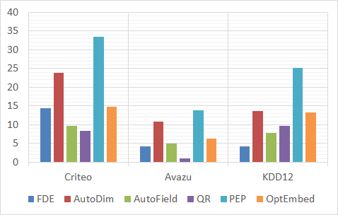
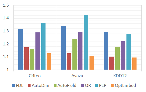
We illustrate the total training and inference time of DeepFM model trained on all three datasets in Fig. 5. Here we define the total training time as the sum of mask searching time(the time required to obtain the embedding and/or dimension mask given different methods) and re-training time(the time for re-training the parameters under the constraint of the embedding and/or dimension mask).
For the total training time in Fig. 5(a), we can observe that QR and AutoField tend to have faster speeds than other methods. For QR, no network architecture search is involved. It also has a smaller embedding table, leading to a faster training speed per epoch. AutoField has a smaller search space than other baselines since it only contains the feature field. Surprisingly, the total training time of original model is not always the fastest. This is because original model may take more epochs to converge. OptEmbed is faster than PEP and AutoDim because they have respectively slower convergence speeds during the mask searching and re-training phase.
The inference time is crucial when deploying the model in reality. As shown in Fig. 5(b), OptEmbed achieves the least inference time. This is because the final embedding table obtained by OptEmbed has the least parameters. PEP requires the longest inference time, even longer than original model, because its embedding table tends to be sparse and hardware-unfriendly. Note that it is inevitable to cost additional time to search masks for OptEmbed. However, the cost is worth considering the performance increase and inference time saving, which are more important in practice.
4.5.2. Space Complexity
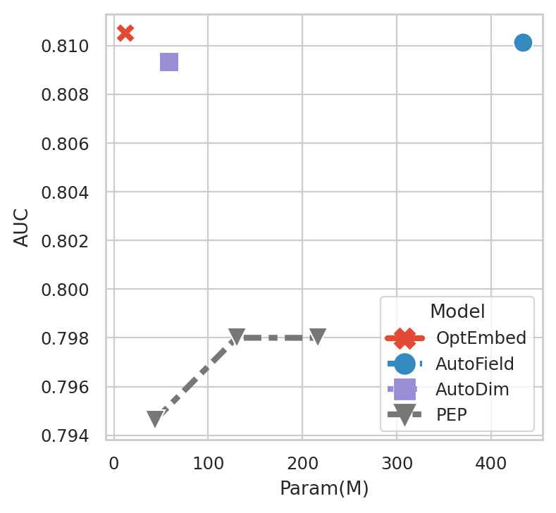
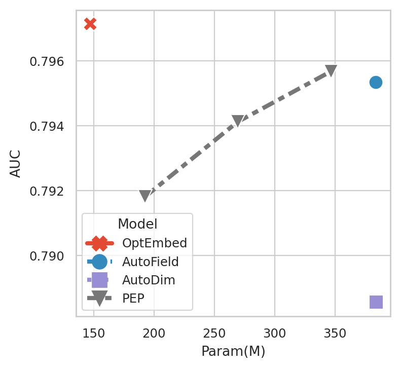
We plot the parameter-AUC curve of the DeepFM model on both Criteo and KDD12 datasets in Fig. 6, which reflects the relationship between the space complexity of the embedding table and model performance. There are multiple PEP points as it requires predetermined sparsity ratios as stopping criteria. So we can easily control the final sparsity ratio. AutoDim, AutoField and OptEmbed primarily aim to improve model performance. However, there is no guarantee of the final sparsity ratio. Hence we only plot one point for each method. From Fig. 6 we can make the following observations: (i) OptEmbed outperforms other baselines with the highest AUC score and the smallest embedding size. (ii) Model performance of PEP tends to degrade with the decrease of embedding parameters. (iii) AutoDim and AutoField only optimize the embedding table along one axis. Hence they do not have stable performance among datasets. They perform well on the Criteo dataset. However, they are surpassed by PEP on the KDD12 dataset.
4.6. Case Study(RQ5)
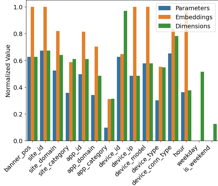
This section uses a case study to investigate the optimal embedding table obtained from OptEmbed. We select the embedding table of FNN model trained on Avazu dataset as an example and exclude all anonymous feature fields. Criteo and KDD12 datasets are not selected because all fields are anonymous. In Fig. 7, we plot total parameters, embedding numbers, dimensions and normalize them with corresponding values from original model, respectively. We can make the following observations. First, each field’s optimal dimensions and remaining feature values vary from one to another. This highlights the necessity for OptEmbed. Second, id-like features (like site_id, app_id, device_id) tend to have higher values than others. Such an observation is consistent with human intuition as the id-like features are the core of collaborative filtering-based recommender system. Third, it is surprising to find out that no embedding is assigned for the weekday and is_weekday fields. These two fields are manually created following the best practice (Zhu et al., 2021). However, their contained information is more likely to be covered by the hour field. Such an observation shows the limit of human-defined feature selection methods.
5. related work
We discuss how our work is situated in two research topics: CTR prediction and embedding table optimization. Many machine learning models have been developed for CTR prediction (Chapelle et al., 2015; Richardson et al., 2007; Rendle, 2010). Due to the powerful learning ability, the mainstream CTR prediction research is dominated by deep learning models (Zhu et al., 2021; Naumov et al., 2019). Wide&Deep (Cheng et al., 2016) and FNN (Zhang et al., 2016) introduce an embedding table to transform the raw inputs and an MLP layer to model high-level representations. DeepFM (Guo et al., 2017), DCN (Wang et al., 2017) and IPNN (Qu et al., 2018) rely on various feature interaction layers to improve performance. Increasing research focus on how to model complex feature interaction (Liu et al., 2020b; Khawar et al., 2020; Lyu et al., 2021). With AutoML technique, AutoFIS (Liu et al., 2020b) and AutoFeature (Khawar et al., 2020) search for feature interaction instead of modeling with implicit layer. OptEmbed is perpendicular to all these researches by providing an optimal embedidng table for various base models.
Studies on optimizing embedding tables can mainly be categorized into reducing memory usage, searching embedding dimensions, and pruning redundant values. Hash embedding (Weinberger et al., 2009) designs a hash method to reduce the embedding table size. Double hash (Zhang et al., 2020) adopts the double hash method for one feature value to reduce the collision in hashing method. Q-R trick (Shi et al., 2020) is also introduced to conquer the collision problem. Some quantized techniques (Kang et al., 2020; Jiang et al., 2021) are also borrowed for compressing the embedding table. To search field-wise embedding dimension, NAS has been utilized automatically based on well-defined search space (Zhao et al., 2021; Ginart et al., 2021; Cheng et al., 2020). NAS has also been utilized to search informative feature field (Wang et al., 2022) automatically. AutoIAS (Wei et al., 2021) introduces a one-shot search for both embedding dimension and architecture. Pruning redundant values in embedding tables attracted more attention recently. PEP (Liu et al., 2021) designs a soft threshold method to filter out low magnitude values in the embedding table with a predetermined sparsity ratio. DeepLight (Deng et al., 2021) prune embedding table and other components on a pre-train network. The single-shot (Qu et al., 2022) pruning method is also used to prune the embedding table carefully. This paper proposes three requirements for an optimal embedding table in Req. 1, 2 and 3, and make a thorough comparison with these works. To the best of our knowledge, we are the first to design an optimal embedding framework satisfying three requirements for CTR prediction.
6. conclusion
This paper first proposes the requirements for an optimal embedding table. Based on these requirements, a novel, model-agnostic framework OptEmbed is proposed. OptEmbed optimizes the embedding table in a unifying way. It is capable of combining the supernet parameter training with redundant embedding pruning. A one-shot embedding search method is proposed based on the supernet to efficiently find optimal dimensions for different fields and obtain the optimal embedding table. Extensive experiments on three large-scale datasets demonstrate the superiority of OptEmbed in terms of both model performance and model size reduction. Several ablation studies demonstrate that basic models require optimal embedding tables on various datasets. Moreover, we also interpret the obtained result on feature fields, highlighting that our method learns the optimal embedding table.
Acknowledgements.
We specifically want to thanks Dr. Jin Guo for her helpful suggestions regarding the paper writing.References
- (1)
- Bender et al. (2018) Gabriel Bender, Pieter-Jan Kindermans, Barret Zoph, Vijay Vasudevan, and Quoc Le. 2018. Understanding and Simplifying One-Shot Architecture Search. In Proceedings of the 35th International Conference on Machine Learning (Proceedings of Machine Learning Research, Vol. 80), Jennifer Dy and Andreas Krause (Eds.). PMLR, Stockholmsmässan, Stockholm, Sweden, 550–559.
- Cai et al. (2019) Han Cai, Ligeng Zhu, and Song Han. 2019. ProxylessNAS: Direct Neural Architecture Search on Target Task and Hardware. In 7th International Conference on Learning Representations, ICLR 2019. OpenReview.net, New Orleans, LA, USA, 13 pages.
- Chapelle et al. (2015) Olivier Chapelle, Eren Manavoglu, and Romer Rosales. 2015. Simple and Scalable Response Prediction for Display Advertising. ACM Trans. Intell. Syst. Technol. 5, 4 (dec 2015), 61.
- Cheng et al. (2016) Heng-Tze Cheng, Levent Koc, Jeremiah Harmsen, Tal Shaked, Tushar Chandra, Hrishi Aradhye, Glen Anderson, Greg Corrado, Wei Chai, Mustafa Ispir, Rohan Anil, Zakaria Haque, Lichan Hong, Vihan Jain, Xiaobing Liu, and Hemal Shah. 2016. Wide & Deep Learning for Recommender Systems. In Proceedings of the 1st Workshop on Deep Learning for Recommender Systems, DLRS@RecSys 2016. ACM, Boston, MA, USA, 7–10.
- Cheng et al. (2020) Weiyu Cheng, Yanyan Shen, and Linpeng Huang. 2020. Differentiable Neural Input Search for Recommender Systems. CoRR abs/2006.04466 (2020).
- Deng et al. (2021) Wei Deng, Junwei Pan, Tian Zhou, Deguang Kong, Aaron Flores, and Guang Lin. 2021. DeepLight: Deep Lightweight Feature Interactions for Accelerating CTR Predictions in Ad Serving. In WSDM ’21. ACM, Virtual Event, Israel, 922–930.
- Donà and Gallinari (2021) Jérémie Donà and Patrick Gallinari. 2021. Differentiable Feature Selection, A Reparameterization Approach. In Machine Learning and Knowledge Discovery in Databases. Research Track. Springer International Publishing, Spain, 414–429.
- Frankle and Carbin (2019) Jonathan Frankle and Michael Carbin. 2019. The Lottery Ticket Hypothesis: Finding Sparse, Trainable Neural Networks. In 7th International Conference on Learning Representations, ICLR 2019. OpenReview.net, New Orleans, LA, USA, 42 pages.
- Ginart et al. (2021) Antonio A. Ginart, Maxim Naumov, Dheevatsa Mudigere, Jiyan Yang, and James Zou. 2021. Mixed Dimension Embeddings with Application to Memory-Efficient Recommendation Systems. In IEEE International Symposium on Information Theory, ISIT 2021. IEEE, Australia, 2786–2791.
- Glorot and Bengio (2010) Xavier Glorot and Yoshua Bengio. 2010. Understanding the difficulty of training deep feedforward neural networks. In Proceedings of the Thirteenth International Conference on Artificial Intelligence and Statistics, AISTATS 2010 (JMLR Proceedings, Vol. 9). JMLR.org, Italy, 249–256.
- Guo et al. (2021) Huifeng Guo, Wei Guo, Yong Gao, Ruiming Tang, Xiuqiang He, and Wenzhi Liu. 2021. ScaleFreeCTR: MixCache-Based Distributed Training System for CTR Models with Huge Embedding Table. Association for Computing Machinery, New York, NY, USA, 1269–1278.
- Guo et al. (2017) Huifeng Guo, Ruiming Tang, Yunming Ye, Zhenguo Li, and Xiuqiang He. 2017. DeepFM: A Factorization-Machine based Neural Network for CTR Prediction. In Proceedings of the Twenty-Sixth International Joint Conference on Artificial Intelligence, IJCAI 2017. ijcai.org, Australia, 1725–1731.
- Guo et al. (2020) Zichao Guo, Xiangyu Zhang, Haoyuan Mu, Wen Heng, Zechun Liu, Yichen Wei, and Jian Sun. 2020. Single Path One-Shot Neural Architecture Search with Uniform Sampling. In Computer Vision - ECCV 2020 - 16th European Conference (Lecture Notes in Computer Science, Vol. 12361). Springer, UK, 544–560.
- Han et al. (2015) Song Han, Jeff Pool, John Tran, and William J. Dally. 2015. Learning both Weights and Connections for Efficient Neural Network. In Advances in Neural Information Processing Systems 28: Annual Conference on Neural Information Processing Systems 2015. Springer, Canada, 1135–1143.
- He and Chua (2017) Xiangnan He and Tat-Seng Chua. 2017. Neural Factorization Machines for Sparse Predictive Analytics. In Proceedings of the 40th International ACM SIGIR Conference on Research and Development in Information Retrieval, Noriko Kando, Tetsuya Sakai, Hideo Joho, Hang Li, Arjen P. de Vries, and Ryen W. White (Eds.). ACM, Shinjuku, Tokyo, Japan, 355–364.
- Ioffe and Szegedy (2015) Sergey Ioffe and Christian Szegedy. 2015. Batch Normalization: Accelerating Deep Network Training by Reducing Internal Covariate Shift. In Proceedings of the 32nd International Conference on Machine Learning, ICML 2015 (JMLR Workshop and Conference Proceedings, Vol. 37). JMLR.org, France, 448–456.
- Jiang et al. (2021) Gangwei Jiang, Hao Wang, Jin Chen, Haoyu Wang, Defu Lian, and Enhong Chen. 2021. xLightFM: Extremely Memory-Efficient Factorization Machine. In SIGIR ’21: The 44th International ACM SIGIR Conference on Research and Development in Information Retrieval, Fernando Diaz, Chirag Shah, Torsten Suel, Pablo Castells, Rosie Jones, and Tetsuya Sakai (Eds.). ACM, Virtual Event, Canada, 337–346.
- Kang et al. (2020) Wang-Cheng Kang, Derek Zhiyuan Cheng, Ting Chen, Xinyang Yi, Dong Lin, Lichan Hong, and Ed H. Chi. 2020. Learning Multi-granular Quantized Embeddings for Large-Vocab Categorical Features in Recommender Systems. In Companion of The 2020 Web Conference 2020. ACM / IW3C2, Taiwan, 562–566.
- Khawar et al. (2020) Farhan Khawar, Xu Hang, Ruiming Tang, Bin Liu, Zhenguo Li, and Xiuqiang He. 2020. AutoFeature: Searching for Feature Interactions and Their Architectures for Click-through Rate Prediction. In CIKM ’20: The 29th ACM International Conference on Information and Knowledge Management. ACM, Ireland, 625–634.
- Liu et al. (2020b) Bin Liu, Chenxu Zhu, Guilin Li, Weinan Zhang, Jincai Lai, Ruiming Tang, Xiuqiang He, Zhenguo Li, and Yong Yu. 2020b. AutoFIS: Automatic Feature Interaction Selection in Factorization Models for Click-Through Rate Prediction. In KDD ’20: The 26th ACM SIGKDD Conference on Knowledge Discovery and Data Mining. ACM, USA, 2636–2645.
- Liu et al. (2019) Hanxiao Liu, Karen Simonyan, and Yiming Yang. 2019. DARTS: Differentiable Architecture Search. In 7th International Conference on Learning Representations, ICLR 2019. OpenReview.net, USA.
- Liu et al. (2020a) Junjie Liu, Zhe Xu, Runbin Shi, Ray C. C. Cheung, and Hayden Kwok-Hay So. 2020a. Dynamic Sparse Training: Find Efficient Sparse Network From Scratch With Trainable Masked Layers. In 8th International Conference on Learning Representations, ICLR 2020. OpenReview.net, Ethiopia. https://openreview.net/forum?id=SJlbGJrtDB
- Liu et al. (2021) Siyi Liu, Chen Gao, Yihong Chen, Depeng Jin, and Yong Li. 2021. Learnable Embedding sizes for Recommender Systems. In 9th International Conference on Learning Representations, ICLR 2021. OpenReview.net, Austria.
- Lyu et al. (2021) Fuyuan Lyu, Xing Tang, Huifeng Guo, Ruiming Tang, Xiuqiang He, Rui Zhang, and Xue Liu. 2021. Memorize, Factorize, or be Naïve: Learning Optimal Feature Interaction Methods for CTR Prediction. CoRR abs/2108.01265 (2021). arXiv:2108.01265 https://arxiv.org/abs/2108.01265
- Meng et al. (2021) Ze Meng, Jinnian Zhang, Yumeng Li, Jiancheng Li, Tanchao Zhu, and Lifeng Sun. 2021. A General Method For Automatic Discovery of Powerful Interactions In Click-Through Rate Prediction. In SIGIR ’21: The 44th International ACM SIGIR Conference on Research and Development in Information Retrieval. ACM, Canada, 1298–1307.
- Naumov et al. (2019) Maxim Naumov, Dheevatsa Mudigere, Hao-Jun Michael Shi, Jianyu Huang, Narayanan Sundaraman, Jongsoo Park, Xiaodong Wang, Udit Gupta, Carole-Jean Wu, Alisson G. Azzolini, Dmytro Dzhulgakov, Andrey Mallevich, Ilia Cherniavskii, Yinghai Lu, Raghuraman Krishnamoorthi, Ansha Yu, Volodymyr Kondratenko, Stephanie Pereira, Xianjie Chen, Wenlin Chen, Vijay Rao, Bill Jia, Liang Xiong, and Misha Smelyanskiy. 2019. Deep Learning Recommendation Model for Personalization and Recommendation Systems. CoRR abs/1906.00091 (2019).
- Qu et al. (2022) Liang Qu, Yonghong Ye, Ningzhi Tang, Lixin Zhang, Yuhui Shi, and Hongzhi Yin. 2022. Single-shot Embedding Dimension Search in Recommender System. CoRR abs/2204.03281 (2022), 11 pages. https://doi.org/10.48550/arXiv.2204.03281 arXiv:2204.03281
- Qu et al. (2018) Yanru Qu, Bohui Fang, Weinan Zhang, Ruiming Tang, Minzhe Niu, Huifeng Guo, Yong Yu, and Xiuqiang He. 2018. Product-Based Neural Networks for User Response Prediction over Multi-Field Categorical Data. ACM Trans. Inf. Syst. 37, 1, Article 5 (oct 2018), 35 pages.
- Rendle (2010) Steffen Rendle. 2010. Factorization Machines. In ICDM 2010, The 10th IEEE International Conference on Data Mining. IEEE Computer Society, Australia, 995–1000.
- Richardson et al. (2007) Matthew Richardson, Ewa Dominowska, and Robert Ragno. 2007. Predicting Clicks: Estimating the Click-through Rate for New Ads. In Proceedings of the 16th International Conference on World Wide Web (Banff, Alberta, Canada) (WWW ’07). Association for Computing Machinery, New York, NY, USA, 521–530.
- Shen et al. (2021) Jiayi Shen, Haotao Wang, Shupeng Gui, Jianchao Tan, Zhangyang Wang, and Ji Liu. 2021. UMEC: Unified model and embedding compression for efficient recommendation systems. In 9th International Conference on Learning Representations, ICLR 2021. OpenReview.net, Austria.
- Shi et al. (2020) Hao-Jun Michael Shi, Dheevatsa Mudigere, Maxim Naumov, and Jiyan Yang. 2020. Compositional Embeddings Using Complementary Partitions for Memory-Efficient Recommendation Systems. In KDD ’20: The 26th ACM SIGKDD Conference on Knowledge Discovery and Data Mining. ACM, USA, 165–175.
- Song et al. (2019) Weiping Song, Chence Shi, Zhiping Xiao, Zhijian Duan, Yewen Xu, Ming Zhang, and Jian Tang. 2019. AutoInt: Automatic Feature Interaction Learning via Self-Attentive Neural Networks. In Proceedings of the 28th ACM International Conference on Information and Knowledge Management, CIKM 2019. ACM, China, 1161–1170.
- Wang et al. (2017) Ruoxi Wang, Bin Fu, Gang Fu, and Mingliang Wang. 2017. Deep & Cross Network for Ad Click Predictions. In Proceedings of the ADKDD’17 (ADKDD’17). Association for Computing Machinery, Canada, Article 12, 7 pages.
- Wang et al. (2022) Yejing Wang, Xiangyu Zhao, Tong Xu, and Xian Wu. 2022. AutoField: Automating Feature Selection in Deep Recommender Systems. In Proceedings of the ACM Web Conference 2022 (Virtual Event, Lyon, France) (WWW ’22). Association for Computing Machinery, New York, NY, USA, 1977–1986.
- Wei et al. (2021) Zhikun Wei, Xin Wang, and Wenwu Zhu. 2021. AutoIAS: Automatic Integrated Architecture Searcher for Click-Trough Rate Prediction. In CIKM ’21: The 30th ACM International Conference on Information and Knowledge Management. ACM, Australia, 2101–2110.
- Weinberger et al. (2009) Kilian Weinberger, Anirban Dasgupta, John Langford, Alex Smola, and Josh Attenberg. 2009. Feature Hashing for Large Scale Multitask Learning. In Proceedings of the 26th Annual International Conference on Machine Learning (Montreal, Quebec, Canada) (ICML ’09). Association for Computing Machinery, New York, NY, USA, 1113–1120. https://doi.org/10.1145/1553374.1553516
- Yan et al. (2021a) Bencheng Yan, Pengjie Wang, Jinquan Liu, Wei Lin, Kuang-Chih Lee, Jian Xu, and Bo Zheng. 2021a. Binary Code Based Hash Embedding for Web-Scale Applications. Association for Computing Machinery, New York, NY, USA, 3563–3567.
- Yan et al. (2021b) Bencheng Yan, Pengjie Wang, Kai Zhang, Wei Lin, Kuang-Chih Lee, Jian Xu, and Bo Zheng. 2021b. Learning Effective and Efficient Embedding via an Adaptively-Masked Twins-based Layer. In CIKM ’21: The 30th ACM International Conference on Information and Knowledge Management. ACM, Australia, 3568–3572.
- Yuan et al. (2021) Xin Yuan, Pedro Henrique Pamplona Savarese, and Michael Maire. 2021. Growing Efficient Deep Networks by Structured Continuous Sparsification. In 9th International Conference on Learning Representations, ICLR 2021. OpenReview.net, Austria. https://openreview.net/forum?id=wb3wxCObbRT
- Zhang et al. (2020) Caojin Zhang, Yicun Liu, Yuanpu Xie, Sofia Ira Ktena, Alykhan Tejani, Akshay Gupta, Pranay Kumar Myana, Deepak Dilipkumar, Suvadip Paul, Ikuhiro Ihara, Prasang Upadhyaya, Ferenc Huszar, and Wenzhe Shi. 2020. Model Size Reduction Using Frequency Based Double Hashing for Recommender Systems. Association for Computing Machinery, New York, NY, USA, 521–526.
- Zhang et al. (2016) Weinan Zhang, Tianming Du, and Jun Wang. 2016. Deep Learning over Multi-field Categorical Data - - A Case Study on User Response Prediction. In Advances in Information Retrieval - 38th European Conference on IR Research, ECIR 2016, Vol. 9626. Springer, Italy, 45–57. https://doi.org/10.1007/978-3-319-30671-1_4
- Zhao et al. (2021) Xiangyu Zhao, Haochen Liu, Hui Liu, Jiliang Tang, Weiwei Guo, Jun Shi, Sida Wang, Huiji Gao, and Bo Long. 2021. AutoDim: Field-aware Embedding Dimension Searchin Recommender Systems. In WWW ’21: The Web Conference 2021. ACM / IW3C2, Slovenia, 3015–3022.
- Zhu et al. (2021) Jieming Zhu, Jinyang Liu, Shuai Yang, Qi Zhang, and Xiuqiang He. 2021. Open Benchmarking for Click-Through Rate Prediction. In Proceedings of the 30th ACM International Conference on Information & Knowledge Management. Association for Computing Machinery, Australia, 2759–2769.