Perimeter control in a mixed bimodal bathtub model

Abstract

Perimeter control involves monitoring network-wide traffic and regulating traffic inflow to alleviate hypercongestion. Implementation of transit priority with perimeter control measures, which allow transit into a controlled area without queuing at the perimeter boundary, is an effective strategy in bimodal transportation systems. However, travelers’ behavior changes in response to perimeter control strategies, such as shifts in their departure times and transportation modes, have not been fully investigated. Therefore, important questions remain, such as the use of transit during perimeter control with transit priority. This paper examines the travelers’ behavior changes in response to perimeter control with transit priority in a mixed bimodal transportation system with cars and flexible route transit (FRT) vehicles. We model departure time and transportation mode choices in such a transportation system with hypercongestion and discomfort in FRT (called the mixed bimodal bathtub model). Initially, we investigate the properties of dynamic user equilibrium without perimeter control. Then, we study the equilibrium patterns during perimeter control with transit priority. Unlike existing works, we find that the number of FRT passengers decreases with time toward the desired arrival time and that FRT may not be used around the peak of rush hour. Furthermore, transit priority may not be sufficient to promote the use of FRT, and additional incentive such as subsidy for lower fares may be required to encourage FRT use during perimeter control. Finally, we show that operating many FRT vehicles does not always decrease the equilibrium cost, even under perimeter control with transit priority.

1 Introduction

1.1 Background

Traffic demand is highly concentrated during the rush hour in urban cities with limited spaces. Consequently, hypercongestion occurs in road networks of many cities (Geroliminis and Daganzo, 2008; Loder et al., 2017). Increased vehicle inflow leads to lower throughput in the hypercongested state, and this externality causes inefficient use of transportation systems. To address this issue, cities have introduced public transportation systems as an alternative mode that can carry more passengers using less urban space than private vehicles. A flexible door-to-door transit system has been proposed as an alternative to transitional fixed-route-based transit to promote the use of transit (Vansteenwegen et al., 2022). However, in some of these cities, the increases in the use of public transportation is causing considerable inconvenience, such as long waiting times at stations or stops (Basso et al., 2019). In particular, public transit vehicles, such as buses, encounter hypercongestion in road networks in addition to such inconvenience. These externalities play an important role in travelers’ decision making (Tirachini et al., 2014; Basso et al., 2019). Under these circumstances, commuters choose their trip timing (departure time) and transportation mode during rush hour in urban cities, where multiple transportation modes interact with each other and share limited urban spaces. Therefore, efficient multimodal transportation systems need to be developed.

Substantial effort has been devoted to management strategies designed to alleviate these externalities. A common strategy is congestion pricing, which promotes travel behavior changes, such as trip timing and transportation mode shifts. Despite the large body of literature on this subject (e.g., Yang and Huang (2005)), it is practically difficult to implement such pricing schemes due to public acceptance (Giuliano, 1992; Gu et al., 2018).

Perimeter control, which regulates traffic inflow into a targeted area by gating or traffic signal control to maintain good traffic conditions, is an alternative strategy of mitigating hypercongestion. Real-time perimeter control is enabled by monitoring the network-wide traffic state based on recent advances in traffic theories, more precisely the macroscopic fundamental diagram (MFD) (Daganzo, 2007). Perimeter control for multimodal transportation systems has been investigated (e.g., Ampountolas et al. (2017) and Haitao et al. (2019)). Haitao et al. (2019) showed that the combination of perimeter control and transit priority is effective in bimodal systems in terms of passenger flow. However, travelers’ behavior changes in response to such strategies, such as shifts in trip timing and transportation modes, have not been fully investigated. Perimeter control is intended to promote trip timing changes (to avoid queuing at perimeter boundaries) and transportation mode shift from cars to transit (which may aggravate discomfort externalities). Although hypercongestion and discomfort in transit are important for traveler decision making in urban cities (Arnott, 2013; Tirachini et al., 2014; de Palma et al., 2017), the impact of such externalities on the effectiveness of perimeter control has been rarely studied. A critical gap is the lack of a methodology that connects travelers’ departure time and transportation mode choices with the complex traffic flow and passenger dynamics in the implementation of perimeter control.

This paper investigates traveler’s behavior changes in response to perimeter control with transit priority. To this end, we consider a bimodal transportation system that has cars and flexible route transit (FRT) vehicles, which have a fixed route but can pick up passengers at their origins in predetermined areas covered by each FRT line. Then, we model departure time and transportation mode choices in the presence of hypercongestion and FRT discomfort (called the mixed bimodal bathtub model).

First, the dynamic user equilibrium is characterized. Unlike the existing works, we find that the number of FRT passengers decreases with time toward the desired arrival time and that FRT use may not be preferred around the peak of rush hour. Then, we investigate the equilibrium patterns in the implementation of perimeter control with transit priority. Studies indicate that transit priority effectively promotes the transit use (Zheng et al., 2017; Dantsuji et al., 2021), but our results show that transit priority at perimeter boundaries may be insufficient and that added incentives, such as subsidy for lower fares, may be required to encourage FRT use during perimeter control. We also show that operating many FRT vehicles does not always decreases the equilibrium cost, even under perimeter control with transit priority.

1.2 Literature review

MFDs are a powerful tool of describing the network-wide traffic dynamics, which relates network flow (or trip completions) to network density (or accumulation of vehicles). The idea of macroscopic traffic flow theory was proposed by Godfrey (1969) and further investigated by Mahmassani et al. (1987) and Daganzo (2007) and then empirically analyzed by Geroliminis and Daganzo (2008). Traffic management approaches based on MFDs have been studied, such as congestion pricing (Zheng et al., 2012; Simoni et al., 2015; Genser and Kouvelas, 2022) and route guidance (Yildirimoglu et al., 2015, 2018). MFDs have also been utilized for other purposes, such as the dynamic traffic demand estimation (Dantsuji et al., 2022) and network performance indicator (Loder et al., 2019; Hamm et al., 2022). To capture the interaction of dynamics between different transportation modes (e.g., car and bus), Geroliminis et al. (2014) proposed the three-dimensional MFD (3D-MFD), which enables the representation of traffic flow in mixed bimodal networks. The multimodal MFD was empirically analyzed (Loder et al., 2017; Dakic and Menendez, 2018; Fu et al., 2020; Paipuri et al., 2021). Traffic management strategies for bimodal systems have also been studied, such as road space allocation (Zheng and Geroliminis, 2013; Chiabaut, 2015; Zheng et al., 2017), perimeter traffic control (Ampountolas et al., 2017), and pricing (Zheng and Geroliminis, 2020; Dantsuji et al., 2021; Loder et al., 2022).

Perimeter control is a successful application of MFDs to traffic management. The idea of perimeter control is to control the entry flow at the perimeter boundary of a targeted area to maximize the trip completion rate (Daganzo, 2007; Haddad and Shraiber, 2014). It has been extended to the multiregion networks (Geroliminis et al., 2012; Haddad and Geroliminis, 2012; Ramezani et al., 2015), perimeter control with boundary queue (Haddad, 2017; Ni and Cassidy, 2020; Guo and Ban, 2020; Li et al., 2021) and with route guidance (Sirmatel and Geroliminis, 2017; Ding et al., 2017), and in bimodal transportation systems (Ampountolas et al., 2017; Haitao et al., 2019; Chen et al., 2022a). Considerable effort has been dedicated to perimeter control schemes, but the impacts of traveler behavior has been insufficiently explored. Specifically. the effect of departure time and transportation mode shifts on the efficiency of perimeter control has rarely been investigated.

Bathtub models, namely dynamic user equilibrium model for departure time choice in urban cities with hypercongestion, have been examined (Small and Chu, 2003; Geroliminis and Levinson, 2009; Arnott, 2013; Fosgerau and Small, 2013; Amirgholy and Gao, 2017; Arnott and Buli, 2018; Jin, 2020; Vickrey, 2020; Bao et al., 2021; Chen et al., 2022b). Bathtub models have also been extended to heterogeneity in trip length (Fosgerau, 2015; Lamotte and Geroliminis, 2018), cruising-for-parking (Geroliminis, 2015; Liu and Geroliminis, 2016), and staggered work schedules (Yildirimoglu et al., 2021). Simultaneous departure time and transportation mode choices models were also investigated for bimodal transportation systems (Gonzales and Daganzo, 2012, 2013; Gonzales, 2015). However, none of them takes into accounts both hypercongestion and transit discomfort despite the importance of these externalities for traveler behavior, particularly in urban cities with limited spaces (Tirachini et al., 2014).

1.3 Contributions

In summary, our contributions are listed as follows:

• We develop the mixed bimodal bathtub model, which describes commuters’ departure time and transportation model choices in the presence of hypercongestion and transit discomfort.

• We find that the number of FRT passengers decreases with time toward the desired arrival time and that FRT may not be used around the peak of rush hour in contrast to the findings of the existing works.

• We show that transit priority may not be sufficient to promote transit use. Furthermore, we show that additional incentives, such as subsidy for reduced fares, may be required to encourage FRT use during perimeter control and that operating many FRT vehicles does not always decrease the equilibrium cost, even under perimeter control with transit priority.

The remaining of this paper is organized as follows. Section 2 shows the development of the bimodal bathtub model. In Section 3, we characterize the model equilibrium. Section 4 presents the formulation of the bimodal bathtub model during perimeter control with transit priority. The equilibrium conditions during perimeter control are studied in Section 5. Numerical examples of the model are provided in Section 6, and we conclude in Section 7.

2 Bimodal bathtub model

2.1 Model setting

Consider a monocentric city that has central business district (CBD) and suburban zones where cars and FRT service are available for all commuters as transportation modes, as shown in Fig. 1. The CBD zone has homogeneous topological characteristics by proper partitioning methods (e.g., Ji and Geroliminis (2012); Dantsuji et al. (2020)). The congestion pattern is homogeneous over space within the CBD, and the CBD zone exhibits the well-defined bimodal MFD. The congestion dynamics in the CBD is thus described as a bimodal bathtub model, whereas we assume that one can travel at the free-flow speed in the suburban zone.

A fixed number of FRT vehicles are circulated in multiple directions in the suburban zone such that all commuters can access the service. Each FRT line has a predetermined coverage area in the suburban zone and has a base route; passengers ride FRT vehicles at stops, and these vehicles can pick up passengers at their origins, in predetermined areas and drop them off at their destinations. (e.g., Zheng et al. (2018); Sipetas and Gonzales (2021)). All FRT vehicles are coordinated and controlled by an operator to prevent bus bunching (e.g., Daganzo and Pilachowski (2011); Bartholdi III and Eisenstein (2012)). Therefore, we assume that the FRT vehicles are distributed homogeneously over the transit lines such that the number of FRT vehicles in the CBD zone is fixed and time invariant ($\displaystyle n_{F}=n_{F}^{s}+n_{F}^{c}$, where $\displaystyle n_{F}$, $\displaystyle n_{F}^{s}$, and $\displaystyle n_{F}^{c}$ are the total number of FRT vehicles and the numbers of FRT vehicles in the suburban and CBD zones, respectively).

We then assume a fixed number, $\displaystyle N$, of homogeneous commuters who have identical preference and desired arrival time. All of them travel from the suburban zone to the CBD zone by choosing departure times and transportation mode to minimize their travel cost.

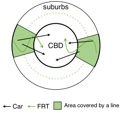
Figure 1: Model structure

2.2 Bimodal bathtub congestion and passenger dynamics of FRT in CBD

To incorporate the bimodal bathtub model of the CBD zone, we extend the Greenshields model to the bimodal congestion dynamics as follows:

$$\displaystyle v_{c}(t) \displaystyle= \displaystyle v_{f}\left(1-\frac{\eta n_{F}(t)+n_{c}(t)}{n_{j}}\right)$$ (1)

$$\displaystyle v_{F}(t) \displaystyle= \displaystyle mv_{c}(t)$$ (2)

where $\displaystyle v_{i}(t)$ is the space-mean speed of transportation mode $\displaystyle i$ ($\displaystyle i\in\{c,F\}$ where $\displaystyle c$ and $\displaystyle F$ represent car and FRT, respectively) at time $\displaystyle t$, $\displaystyle v_{f}$ is the free-flow car space-mean speed, $\displaystyle n_{i}(t)$ is the accumulation of mode $\displaystyle i$’s vehicles in the CBD zone at time $\displaystyle t$, $\displaystyle\eta$ is the passenger car unit, $\displaystyle n_{j}$ is jam accumulation and $\displaystyle m$ indicates that transit vehicles travel slower than cars due to passenger boarding and alighting ($\displaystyle 0<m<1$), which is similar to the modeling of Loder et al. (2017).

As mentioned above, we assume that FRT vehicle accumulation in the CBD zone is fixed; that is $\displaystyle n_{F}(t)=n_{F}^{c}$. Thus, Eq. (1) can be rewritten as

$$\displaystyle v_{c}(t) \displaystyle= \displaystyle v_{f}^{\prime}\left(1-\frac{n_{c}(t)}{n_{j}^{\prime}}\right)$$ (3)

where $\displaystyle v_{f}^{\prime}=v_{f}\left(1-\eta n_{F}^{c}/n_{j}\right)$ and $\displaystyle n_{j}^{\prime}=n_{j}\left(1-\eta n_{F}^{c}/n_{j}\right)$.

Since the CBD is modeled as a system that has inflow and outflow and whose traffic conditions are governed by bathtub congestion dynamics (Daganzo, 2007), the time evolution of car accumulation, $\displaystyle\dot{n_{c}}(t)$, is given by

$$\displaystyle\dot{n_{c}}(t)=I_{c}(t)-G_{c}(t)$$ (4)

where $\displaystyle I_{c}(t)$ is the car inflow rate to the CBD at time $\displaystyle t$ and $\displaystyle G_{c}(t)$ is the car passenger arrival rate at the destination at time $\displaystyle t$. The car passenger arrival rate is formulated by the network exit function (Gonzales and Daganzo, 2012) as

$$\displaystyle G_{c}(t)=\frac{n_{c}(t)v_{c}(t)}{L_{c}}$$ (5)

where $\displaystyle L_{c}$ is the average trip length of the car commuters in the CBD zone.

From the perspective of passenger flow, we assume that all commuters have their own car, and the car commuters travel by their own car (i.e., the occupancy of cars is $\displaystyle 1$ [pax/veh]). With $\displaystyle O_{F}(t)$ denoting the average number of passengers per FRT vehicle at time $\displaystyle t$, the FRT passenger arrival rate, $\displaystyle G_{F}^{p}(t)$, is given by

$$\displaystyle G_{F}^{p}(t)=\frac{O_{F}(t)n_{F}^{c}v_{F}(t)}{L_{F}}$$ (6)

where $\displaystyle L_{F}$ is the average trip length of the FRT commuters in the CBD zone. In analogy with the evolution of car accumulation, the evolution of the average number of the passengers per a FRT vehicle, $\displaystyle\dot{O_{F}}(t)$, is given by

$$\displaystyle\dot{O_{F}}(t)=\frac{1}{n_{F}}\left(d_{F}(t)-\frac{O_{F}(t)n_{F}^{c}v_{F}(t)}{L_{F}}\right)$$ (7)

where $\displaystyle d_{F}(t)$ is the departure rate of FRT passengers at time $\displaystyle t$. The term in the bracket is the difference between the numbers of the passengers boarding and alighting at time $\displaystyle t$. Therefore, the time evolution of $\displaystyle O_{F}(t)$ is calculated by dividing it by the total number of FRT vehicles in the monocentric city, $\displaystyle n_{F}$.

Travel time is time spent in the CBD zone to complete the trip length. Hence, the travel time of each mode $\displaystyle i$ in the CBD zone is

$$\displaystyle\int_{t}^{t+T_{i}(t)}v_{i}(u)du=L_{i},\;\;\;\;i\in\{c,F\}$$ (8)

With Eq.(8), the departure time choice model in the bathtub is intractable (Arnott, 2013). Thus, we assume that the travel time in the CBD zone of a commuter who arrives at time $\displaystyle t$ by transportation mode $\displaystyle i$ is approximated by

$$\displaystyle T_{i}(t)\approx\frac{L_{i}}{v_{i}(t)}$$ (9)

There are several ways of the approximation for the tractability in the literature (Arnott, 2013; Fosgerau and Small, 2013). In this study, we assume that the travel time is determined by a single instant of time (Small and Chu, 2003; Geroliminis and Levinson, 2009).

2.3 Travel cost

Given the bathtub congestion dynamics above, the car travel cost incurred by a commuter who arrive at time $\displaystyle t$ is given by

$$\displaystyle C_{c}(t) \displaystyle= \displaystyle\begin{cases}\alpha\left(T_{c}^{s}+T_{c}(t)\right)+\beta\left(t^{*}-t\right)+p_{c}&\text{if }t\leq t^{*}\\ \alpha\left(T_{c}^{s}+T_{c}(t)\right)+\gamma\left(t-t^{*}\right)+p_{c}&\text{if }t>t^{*}\end{cases}$$ (10)

where $\displaystyle T_{c}^{s}$ is the free-flow car travel time in the suburban zone, $\displaystyle T_{c}(t)$ is the travel time in the CBD zone, as defined by Eq.(9) and $\displaystyle t^{*}$ is the desired arrival time. We assume that commuters have “$\displaystyle\alpha$ - $\displaystyle\beta$ - $\displaystyle\gamma$” type preference (Arnott et al., 1993). The first, second, and third terms of the RHS are the travel time cost, the schedule delay cost, and the car operation cost (e.g., parking fee, gasoline expense), respectively. The travel time in the suburban zone and the car operation cost are time invariant. For simplicity, we combine the two costs as $\displaystyle F_{c}$ (i.e., $\displaystyle F_{c}=\alpha T_{c}^{s}+p_{c}$) to obtain

$$\displaystyle C_{c}(t) \displaystyle= \displaystyle\begin{cases}\alpha T_{c}(t)+\beta\left(t^{*}-t\right)+F_{c}&\text{if }t\leq t^{*}\\ \alpha T_{c}(t)+\gamma\left(t-t^{*}\right)+F_{c}&\text{if }t>t^{*}\end{cases}$$ (11)

The FRT travel cost incurred by a commuter who arrives at time $\displaystyle t$ is

$$\displaystyle C_{F}(t) \displaystyle= \displaystyle\begin{cases}\alpha\left(T_{F}^{s}+T_{F}(t)\right)+\beta\left(t^{*}-t\right)+g(t)+p_{F}&\text{if }t\leq t^{*}\\ \alpha\left(T_{F}^{s}+T_{F}(t)\right)+\gamma\left(t-t^{*}\right)+g(t)+p_{F}&\text{if }t>t^{*}\end{cases}$$ (12)

where $\displaystyle T_{F}^{s}$ is the free-flow FRT travel time in the suburban zone, $\displaystyle T_{F}(t)$ is the FRT travel time in the CBD zone, as defined by Eq. (9), $\displaystyle g(t)$ is the discomfort cost at time $\displaystyle t$ and $\displaystyle p_{F}$ is the FRT fare. In addition to travel time and schedule delay costs, an FRT commuter incurs the discomfort cost and the FRT fare. For simplicity, the discomfort cost incurred by an FRT commuter is assumed to be proportional to the average number of passengers per FRT vehicle when this commuter arrives at their destinations.

$$\displaystyle g(t)=\lambda O_{F}(t)$$ (13)

where $\displaystyle\lambda$ is the marginal disutility of the discomfort, $\displaystyle O_{F}(t)$ is the average number of passengers per FRT vehicle at time $\displaystyle t$. This assumption indicates that discomfort in FRT is related to the number of passengers in the FRT vehicles. It can represent the waiting time for pickup (Basso et al., 2019) or the boarding and alighting times of other passengers. A linear function is commonly assumed for the discomfort cost (Wu and Huang, 2014; Xu et al., 2018). Futhermore, the assumption that this cost is proportional to the average number of passengers per FRT vehicle when a commuter arrives at their destination is consistent with the travel time assumption (the travel time is determined by the arrival time at the destination (Eq. (9)).

By combining the travel cost in the suburban zone and the FRT fare (i.e., $\displaystyle F_{F}=\alpha T_{F}^{s}+p_{F}$), we obtain

$$\displaystyle C_{F}(t) \displaystyle= \displaystyle\begin{cases}\alpha T_{F}(t)+\beta\left(t^{*}-t\right)+\lambda O_{F}(t)+F_{F}&\text{if }t\leq t^{*}\\ \alpha T_{F}(t)+\gamma\left(t-t^{*}\right)+\lambda O_{F}(t)+F_{F}&\text{if }t>t^{*}\end{cases}$$ (14)

Additionally, to analyze the equilibrium when both modes are used during rush hour, we assume that the average FRT trip length is longer than that of a car (i.e., $\displaystyle L_{F}>L_{c}$), and that the marginal cost of earliness is less than that of the travel time (i.e., $\displaystyle\beta<\alpha$) for the FIFO property.

3 Equilibrium

We define dynamic user equilibrium following Wardrop (1952)’s first principle. That is, at equilibrium, no commuter can reduce their travel cost by changing their departure time and transportation mode. The equilibrium conditions are

$$\displaystyle\begin{cases}C_{c}(t)=c^{*}&\text{if }n_{c}(t)>0\\ C_{c}(t)\geq c^{*}&\text{if }n_{c}(t)=0\\ \end{cases}\;\;\;\forall t\in\mathbb{R}$$ (15a)

$$\displaystyle\begin{cases}C_{F}(t)=c^{*}&\text{if }O_{F}(t)>0\\ C_{F}(t)\geq c^{*}&\text{if }O_{F}(t)=0\\ \end{cases}\;\;\;\forall t\in\mathbb{R}$$ (15b)

$$\displaystyle\int_{t\in\mathbb{R}}\frac{n_{c}(s)v_{c}(s)}{L_{c}}ds+\int_{t\in\mathbb{R}}\frac{O_{F}(s)n_{F}^{c}v_{F}(s)}{L_{F}}ds=N$$ (15c)

where $\displaystyle c^{*}$ is the equilibrium cost. Condition (15a) states that if the car travel cost at time $\displaystyle t$ is greater than the equilibrium cost, no one will arrive at their destination by car at time $\displaystyle t$. According to Condition (15b), if the FRT travel cost at time $\displaystyle t$ is greater than the equilibrium cost, no one will take FRT at time $\displaystyle t$. Condition (15c) is the conservation law for travel demand: integrating the arrival rate is total number of commuters.

3.1 Equilibrium properties

Let [$\displaystyle t_{s}^{c}$, $\displaystyle t_{e}^{c}$] and [$\displaystyle t_{s}^{F}$, $\displaystyle t_{e}^{F}$] be the time windows between the first and last commuters who arrive at their destinations by car and FRT, respectively. That is, these time windows represent the rush hour of each transportation mode. We define $\displaystyle\theta\equiv\frac{(c^{*}-F_{c})v_{f}^{{}^{\prime}}}{\alpha L_{c}}$ which is the ratio of the sum of the travel time and schedule delay costs at equilibrium to the free-flow travel time (sum of travel time and schedule delay costs at equilibrium when the number of car commuters is zero) (Arnott, 2013). It represents the duration of the car rush hour (or the severity of traffic congestion); that is, the larger the $\displaystyle\theta$, the longer the car rush hour. We present the following proposition on the equilibrium when both modes are used.

Proposition 1.

If $\displaystyle\theta>1$ and $\displaystyle\Delta F>\alpha\Delta T_{f}$ where $\displaystyle\Delta F=F_{c}-F_{F}$ and $\displaystyle\Delta T_{f}=L_{F}/mv_{f}^{\prime}-L_{c}/v_{f}^{\prime}$ , then both modes are used during rush hour, and the FRT rush hour starts earlier and ends later than the car rush hour. If $\displaystyle\Delta F\leq\alpha\Delta T_{f}$, FRT is never used. If $\displaystyle\theta\leq 1$, cars are never used.

Proof.

As shown in Small and Chu (2003), the time evolution of car accumulation at equilibrium with Eq. (9) is given by

$$\displaystyle n_{c}(t)=\begin{cases}n_{j}^{\prime}\left(1-\frac{1}{1+\frac{\beta}{\alpha T_{f}^{c}}\left(t-t_{s}^{c}\right)}\right)&\text{if }t\leq t^{*}\\ n_{j}^{\prime}\left(1-\frac{1}{1+\frac{\gamma}{\alpha T_{f}^{c}}\left(t_{e}^{c}-t\right)}\right)&\text{if }t^{*}<t\end{cases}$$ (16)

The first car commuter incurs the travel time cost at free-flow in the CBD. Thus, the car travel cost at time $\displaystyle t_{s}^{c}$ is given by

$$\displaystyle C_{c}(t_{s}^{c})=\alpha T_{f}^{c}+\beta\left(t^{*}-t_{s}^{c}\right)+F_{c}$$ (17)

where $\displaystyle T_{f}^{c}$ is the car free-flow travel time ($\displaystyle=L_{c}/v_{f}^{\prime}$). The FRT travel cost at time $\displaystyle t_{s}^{c}$ is

$$\displaystyle C_{F}(t_{s}^{c})=\alpha T_{f}^{F}+\beta\left(t^{*}-t_{s}^{c}\right)+\lambda O_{F}(t_{s}^{c})+F_{F}$$ (18)

where $\displaystyle T_{f}^{F}$ is the FRT free-flow travel time ($\displaystyle=L_{F}/mv_{f}^{\prime}$). As seen from Eqs. (2), (3), (9), and (16) that $\displaystyle\frac{dT_{c}(t)}{dt}=\frac{\beta}{\alpha}$ and $\displaystyle\frac{dT_{F}(t)}{dt}=\frac{T_{f}^{F}}{T_{f}^{c}}\frac{\beta}{\alpha}$ for earliness, which yields $\displaystyle\frac{dT_{c}(t)}{dt}<\frac{dT_{F}(t)}{dt}$ by the assumptions that $\displaystyle L_{F}>L_{c}$ and $\displaystyle 0<m<1$, which indicates that the FRT travel time cost increases with time more than the car travel time cost, once the car rush hour starts. Thus, FRT is never used if no one takes FRT at the car rush hour start time, $\displaystyle t_{s}^{c}$. When both modes are used, the FRT travel cost without the discomfort cost is less than the car travel cost at time $\displaystyle t_{s}^{c}$.

$$\displaystyle\alpha T_{f}^{c}+\beta\left(t^{*}-t_{s}^{c}\right)+F_{c}>\alpha T_{f}^{F}+\beta\left(t^{*}-t_{s}^{c}\right)+F_{F}$$ (19)

It yields

$$\displaystyle\Delta F>\alpha\Delta T_{f}$$ (20)

Before the car rush hour starts (travel time is time-invariant at free-flow), we have $\displaystyle\frac{dC_{F}(t)}{dt}=\beta+\lambda\dot{O_{F}}(t)$ from Eq. (14). Then, Condition (15b) yields

$$\displaystyle\dot{O_{F}}(t)=\frac{\beta}{\lambda}$$ (21)

Therefore, the time, $\displaystyle t_{s}^{F}$, when the FRT rush hour starts ($\displaystyle O_{F}(t_{s}^{F})=0$) is earlier than $\displaystyle t_{s}^{c}$. In the same way, we can prove for lateness that $\displaystyle t_{e}^{F}>t_{e}^{c}$.

Obviously, cars are never used if $\displaystyle c^{*}\leq\alpha L_{c}/v_{f}^{\prime}+F_{c}$. This condition can be written by

$$\displaystyle\theta\leq 1$$ (22)

∎

This proposition indicates that both modes will be used if the fixed cost difference ($\displaystyle\Delta F$) is greater than the free-flow travel time cost difference ($\displaystyle\alpha\Delta T_{f}$). As the FRT travel cost is lower than the car travel cost outside both modes’ rush hour, the FRT rush hour starts earlier and ends later. Then, since FRT commuters incur the discomfort cost in addition to the costs they have in common with car commuters (travel time, schedule delay, and fixed costs), there is a time when the car travel cost becomes equal to the FRT travel cost. Thus, both modes will be used. Contrarily, if the fixed cost difference is lower than the free-flow travel cost difference, the FRT travel cost will always be larger than the car travel cost; thus, FRT will not be used. Furthermore, if the car fixed cost and free-flow travel time are too high, no one will use their cars and all commuters will take FRT. Since the travel time is time-invariant at free-flow during the FRT rush hour in this case, the number of FRT passengers increases linearly toward the desired arrival time.

As this study aims to analyze equilibrium patterns when both modes are used, we impose the following assumption for the remainder of this paper.

Assumption 1.

$\displaystyle\theta>1$ and $\displaystyle\Delta F>\alpha\Delta T_{f}$

At equilibrium when both modes are used, we have the following proposition.

Proposition 2.

Suppose Assumption 1. Then, the equilibrium has the following properties.

1. For earliness, the number of FRT passengers increases with time before the car rush hour and begins to decrease toward the desired arrival time once the car rush hour starts. For lateness, it increases after the desired arrival time and starts to decrease after the car rush hour ends.

2. If $\displaystyle\frac{\Delta F}{\alpha\Delta T_{f}}<\theta$, there will be a time window wherein the FRT is not used during the FRT rush hour, and the time window $\displaystyle[t_{ee}^{F},t_{sl}^{F}]$ is given by

   $$\displaystyle t_{ee}^{F}=t_{s}^{c}+\frac{\alpha T_{f}^{c}}{\beta}\frac{\Delta F-\alpha\Delta T_{f}}{\alpha\Delta T_{f}}$$ (23)

   $$\displaystyle t_{sl}^{F}=t_{e}^{c}-\frac{\alpha T_{f}^{c}}{\gamma}\frac{\Delta F-\alpha\Delta T_{f}}{\alpha\Delta T_{f}}$$ (24)

3. If $\displaystyle\frac{\Delta F}{\alpha\Delta T_{f}}\geq\theta$, FRT will be used from the beginning to the end of the FRT rush hour.

Proof.

$\displaystyle\dot{O_{F}}(t)=\beta/\lambda$ if $\displaystyle t_{s}^{F}<t<t_{s}^{c}$, as stated in Eq. (21). Thus, $\displaystyle{O_{F}}(t)$ increases linearly before the car rush hour. During the car rush hour, according to Conditions (15a) and (15b), we have $\displaystyle C_{c}(t)=C_{F}(t)$ when both modes are used. For earliness, combining this with Eqs. (11) and (14) yields

$$\displaystyle O_{F}(t)=\frac{1}{\lambda}\left(\Delta F-\alpha\left(T_{F}(t)-T_{c}(t)\right)\right)$$ (25)

By substituting Eqs. (3), (9), and (16) into Eq. (25), we obtain

$$\displaystyle O_{F}(t)=\frac{1}{\lambda}\left(\Delta F-\alpha\Delta T_{f}\left(1+\frac{\beta}{\alpha T_{f}^{c}}\left(t-t_{s}^{c}\right)\right)\right)$$ (26)

As $\displaystyle\dot{O_{F}}(t)<0$ after the car rush hour starts, $\displaystyle{O_{F}}(t)$ decreases linearly.

For lateness, we have

$$\displaystyle O_{F}(t)=\frac{1}{\lambda}\left(\Delta F-\alpha\Delta T_{f}\left(1+\frac{\gamma}{\alpha T_{f}^{c}}\left(t_{e}^{c}-t\right)\right)\right)$$ (27)

Thus, $\displaystyle{O_{F}}(t)$ increases linearly before the car rush hour ends. Then, $\displaystyle\dot{O_{F}}(t)=-\gamma/\lambda$ for the time after the car rush hour. Therefore, for earliness, the number of FRT passengers increases with time before the car rush hour and decreases toward the desired arrival time once the car rush hour starts. Then, for lateness, it increases after the desired arrival time and decreases after the car rush hour ends.

Since the number of FRT passengers decreases after the car rush hour starts, there may be a time wherein $\displaystyle O_{F}(t)=0$ before the desired arrival time. Let $\displaystyle t_{ee}^{F}$ denote this time. From Eq. (26), we obtain

$$\displaystyle t_{ee}^{F}=t_{s}^{c}+\frac{\alpha T_{f}^{c}}{\beta}\frac{\Delta F-\alpha\Delta T_{f}}{\alpha\Delta T_{f}}$$ (28)

In the same way, we have $\displaystyle t_{sl}^{F}=t_{e}^{c}-\frac{\alpha T_{f}^{c}}{\gamma}\frac{\Delta F-\alpha\Delta T_{f}}{\alpha\Delta T_{f}}$ for lateness.

The use of FRT will continue during the FRT rush hour if $\displaystyle t_{ee}^{F}>t^{*}$. Condition (15a) states that $\displaystyle c^{*}=\alpha T_{f}^{c}+\beta(t^{*}-t_{s}^{c})+F_{c}$, combining this condition with Eq. (28) leads to the following condition for $\displaystyle t_{ee}^{F}<t^{*}$:

$$\displaystyle\frac{\Delta F}{\alpha\Delta T_{f}}<\theta$$ (29)

which completes the proof. ∎

Figure 2: Illustration of Proposition 2.2

Figure 3: Illustration of Proposition 2.3

Propositions 2.2 and 2.3 are depicted in Figs. 2 and 3, respectively. For earliness, the number of FRT passengers increases with time before the car rush hour, as shown in Eq. (21). During the time interval $\displaystyle[t_{s}^{F},t_{s}^{c})$, the only externality that they incur is discomfort. Thus, the trade-off between discomfort and schedule delay causes this increase in FRT passengers with time. As seen from Eq. (26), once the car rush hour starts, the number of FRT passengers begins to decrease; it will become zero at time $\displaystyle t_{ee}^{F}$ (before the desired arrival time) if the fixed cost difference is relatively low compared with the travel time and schedule delay costs ($\displaystyle\Delta F/\alpha\Delta T_{f}<\theta$). Note that as defined above, a large $\displaystyle\theta$ represents a long car rush hour (large travel time around the peak of the rush hour). Since the travel time cost increases due to the increase in car accumulation once the car rush hour starts (Eq. (16)), the discomfort cost has to be decreased to keep the travel cost at the equilibrium cost, and the number of FRT passengers will decrease. Then, FRT will not be used during the time window $\displaystyle t\in[t_{ee}^{F},t_{sl}^{F})$ if $\displaystyle\Delta F/\alpha\Delta T_{f}<\theta$. Similarly, for lateness, the average number of passengers per FRT vehicle increases during the time interval $\displaystyle[t_{sl}^{F},t_{e}^{c}]$ and begins to decrease after the car rush hour. If $\displaystyle\Delta F/\alpha\Delta T_{f}\geq\theta$ (e.g., the fixed car cost is significantly higher than the FRT fixed cost ), there will be no time window wherein FRT is not used, as depicted in Fig. 3.

These results differ from previous findings on bimodal morning commute problems that consider dynamic congestion for transit (or hypercongestion), where transit is used continuously once the transit rush hour starts and the number of transit passengers is constant or increases toward the desired arrival time (Gonzales and Daganzo, 2012; Basso et al., 2019). This difference is caused by the two externalities incorporated in the proposed model. Gonzales and Daganzo (2012) assumed that the transit travel cost is constant by dedicated lanes and did not consider any externality for transit. Basso et al. (2019) considered the externality of the waiting time at bus stops, but transit vehicles in their study were not subjected to bottleneck congestion. Hypercongestion and discomfort in transit (e.g., crowding and waiting time at stops) in urban cities are not negligible (e.g., Tirachini et al. (2014)). Hence, these externalities play a role in commuters’ travel behavior changes. However, empirical measurements that combine urban hypercongestion, discomfort, and transit user travel behavior have not been investigated. Nonetheless, existing estimation methods of hypercongestion (e.g., Geroliminis and Daganzo (2008)) and massive smart IC card data (e.g., Dantsuji et al. (2022)) may reveal those relationships, which is an interesting future direction of the current paper.

3.2 Equilibrium cost

Next, we derive the equilibrium cost for the case where there is a time window when FRT is not used ($\displaystyle\Delta F/\alpha\Delta T_{f}<\theta$) . As derived in Small and Chu (2003), the number of car commuters at equilibrium, $\displaystyle N_{c}$, is

$$\displaystyle N_{c} \displaystyle= \displaystyle\int_{t_{s}^{c}}^{t_{e}^{c}}\frac{n_{c}(s)v_{c}(s)}{L_{c}}ds$$ (30)

$$\displaystyle= \displaystyle n_{j}^{\prime}\left(\frac{\alpha}{\beta}+\frac{\alpha}{\gamma}\right)\left(\ln\theta+\frac{1}{\theta}-1\right)$$

As shown above, we obtain

$$\displaystyle O_{F}(t)=\begin{cases}\frac{\beta}{\lambda}(t-t_{s}^{F})&\text{if }t_{s}^{F}\leq t<t_{s}^{c}\\ \frac{1}{\lambda}\left(\Delta F-\alpha\Delta T_{f}\left(1+\frac{\beta}{\alpha T_{f}^{c}}\left(t-t_{s}^{c}\right)\right)\right)&\text{if }t_{s}^{c}\leq t<t_{ee}^{F}\\ \frac{1}{\lambda}\left(\Delta F-\alpha\Delta T_{f}\left(1+\frac{\gamma}{\alpha T_{f}^{c}}\left(t_{e}^{c}-t\right)\right)\right)&\text{if }t_{ls}^{d}\leq t<t_{e}^{c}\\ \frac{\beta}{\lambda}(t-t_{s}^{F})&\text{if }t_{e}^{c}\leq t<t_{e}^{d}\end{cases}$$ (31)

Therefore, $\displaystyle O_{F}(t_{s}^{c})=O_{F}(t_{e}^{c})=\frac{1}{\lambda}\left(\Delta F-\alpha\Delta T_{f}\right)$, and the FRT rush hour start and end times are

$$\displaystyle t_{s}^{c}-t_{s}^{F}=\frac{1}{\beta}\left(\Delta F-\alpha\Delta T_{f}\right)$$ (32)

$$\displaystyle t_{e}^{F}-t_{e}^{c}=\frac{1}{\gamma}\left(\Delta F-\alpha\Delta T_{f}\right)$$ (33)

We can also derive the FRT speed from Eqs. (2), (3), and (16) as

$$\displaystyle v_{F}(t)=\begin{cases}mv_{f}^{\prime}&\text{if }t<t_{s}^{c}\\ mv_{f}^{\prime}\left(1+\frac{\beta}{\alpha T_{f}^{c}}(t-t_{s}^{c})\right)^{-1}&\text{if }t_{s}^{c}\leq t<t^{*}\\ mv_{f}^{\prime}\left(1+\frac{\gamma}{\alpha T_{f}^{c}}(t_{e}^{c}-t)\right)^{-1}&\text{if }t^{*}\leq t<t_{e}^{c}\\ mv_{f}^{\prime}&\text{if }t_{e}^{c}\leq t\end{cases}$$ (34)

By integrating the arrival rates in these time windows, we determine the total number of FRT commuters at equilibrium as

$$\displaystyle N_{F} \displaystyle= \displaystyle\int_{t_{s}^{F}}^{t_{e}^{F}}\frac{O_{F}(s)n_{F}^{c}v_{F}(s)}{L_{F}}ds$$ (35)

$$\displaystyle= \displaystyle\left(\frac{1}{\beta}+\frac{1}{\gamma}\right)\left(\frac{n_{F}^{c}}{2\lambda}\frac{1}{T_{f}^{F}}\left(\Delta F-\alpha\Delta T_{f}\right)^{2}+n_{F}^{c}\frac{\alpha}{\lambda}\frac{T_{f}^{c}}{T_{f}^{F}}\left(\Delta F\ln\frac{\Delta F}{\alpha\Delta T_{f}}-\left(\Delta F-\alpha\Delta T_{f}\right)\right)\right)$$

From Eqs. (30) and (35), we have

$$\displaystyle N=\left(\frac{1}{\beta}+\frac{1}{\gamma}\right)\left(\alpha n_{j}^{\prime}\left(\ln\theta+\frac{1}{\theta}-1\right)+\frac{n_{F}^{c}}{2\lambda}\frac{1}{T_{f}^{F}}\left(\Delta F-\alpha\Delta T_{f}\right)^{2}+n_{F}^{c}\frac{\alpha}{\lambda}\frac{T_{f}^{c}}{T_{f}^{F}}\left(\Delta F\ln\frac{\Delta F}{\alpha\Delta T_{f}}-\left(\Delta F-\alpha\Delta T_{f}\right)\right)\right)$$ (36)

where $\displaystyle\theta\equiv\frac{(c^{*}-F_{c})v_{f}^{{}^{\prime}}}{\alpha L_{c}}$. As all variables except the equilibrium cost $\displaystyle c^{*}$ are exogenous, the equilibrium cost can be solved numerically as in Small and Chu (2003).

For the case where FRT is continuously used ( $\displaystyle\frac{\Delta F}{\alpha\Delta T_{f}}\geq\theta$), by replacing $\displaystyle t_{ee}^{F}$ and $\displaystyle t_{sl}^{F}$ with $\displaystyle t^{*}$ in Eq. (31), we obtain

$$\displaystyle O_{F}(t)=\begin{cases}\frac{\beta}{\lambda}(t-t_{s}^{F})&\text{if }t_{s}^{F}\leq t<t_{s}^{c}\\ \frac{1}{\lambda}\left(\Delta F-\alpha\Delta T_{f}\left(1+\frac{\beta}{\alpha T_{f}^{c}}\left(t-t_{s}^{c}\right)\right)\right)&\text{if }t_{s}^{c}\leq t<t^{*}\\ \frac{1}{\lambda}\left(\Delta F-\alpha\Delta T_{f}\left(1+\frac{\gamma}{\alpha T_{f}^{c}}\left(t_{e}^{c}-t\right)\right)\right)&\text{if }t^{*}\leq t<t_{e}^{c}\\ \frac{\beta}{\lambda}(t-t_{s}^{F})&\text{if }t_{e}^{c}\leq t<t_{e}^{F}\end{cases}$$ (37)

Thus, the total number of FRT commuters is

$$\displaystyle N_{F} \displaystyle= \displaystyle\int_{t_{s}^{F}}^{t_{e}^{F}}\frac{O_{F}(s)n_{F}^{c}v_{F}(s)}{L_{F}}ds$$ (38)

$$\displaystyle= \displaystyle\left(\frac{1}{\beta}+\frac{1}{\gamma}\right)\left(\frac{n_{F}^{c}}{2\lambda}\frac{1}{T_{f}^{F}}\left(\Delta F-\alpha\Delta T_{f}\right)^{2}+n_{F}^{c}\frac{\alpha}{\lambda}\frac{T_{f}^{c}}{T_{f}^{F}}\left(\Delta F\ln\theta+\alpha\Delta T_{f}\left(\theta-1\right)\right)\right)$$

As the calculation of the number of car commuters is the same as Eq. (30), we have

$$\displaystyle N=\left(\frac{1}{\beta}+\frac{1}{\gamma}\right)\left(\alpha n_{j}^{\prime}\left(\ln\theta+\frac{1}{\theta}-1\right)+\frac{n_{F}^{c}}{2\lambda}\frac{1}{T_{f}^{F}}\left(\Delta F-\alpha\Delta T_{f}\right)^{2}+n_{F}^{c}\frac{\alpha}{\lambda}\frac{T_{f}^{c}}{T_{f}^{F}}\left(\Delta F\ln\theta+\alpha\Delta T_{f}\left(\theta-1\right)\right)\right)$$ (39)

where $\displaystyle\theta\equiv\frac{(c^{*}-F_{c})v_{f}^{{}^{\prime}}}{\alpha L_{c}}$. As in Eq. (36), all parameters except the equilibrium cost $\displaystyle c^{*}$ are exogenous. Therefore, the equilibrium cost can be solved numerically with respect to the equilibrium cost $\displaystyle c^{*}$.

In summary, the equilibrium cost can be solved numerically, regardless of FRT usage, and has the following property:

Proposition 3.

The equilibrium cost is uniquely determined, regardless of the existence of a time window when FRT is not used during the FRT rush hour.

Proof.

See Appendix A. ∎

FRT use is restricted due to hypercongestion and discomfort, particularly around the peak of rush hour. A large share of transit services, such as FRT, is a key component of efficient and, sustainable transportation systems. Therefore, in the next section, we discuss the management strategy of perimeter control with transit priority to promote FRT use.

4 Perimeter control with transit priority

During perimeter control with transit priority, the inflow rate to the CBD is restricted to protect the zone from hypercongestion. Therefore, a queue will develop outside the perimeter boundary if the arrival rate of cars at the boundary exceeds the inflow rate to the CBD zone, whereas FRT vehicles can pass the perimeter boundary freely by using dedicated lanes at the perimeter (Fig. 5). There are certain strategies for perimeter control with transit priority. One example is similar to the strategy proposed by Haitao et al. (2019). In their strategy, a pre-signal is installed at the upstream point of the main traffic signal to control the inflow into the CBD zone, and the lanes are separated between cars and FRT vehicles at the upstream link of the pre-signal point as depicted in Fig. 5. The strategy is that the pre-signal for FRT stays green, whereas that for cars turns from green to red for perimeter control to maintain the maximum throughput in the CBD zone. Thus, the FRT vehicles can pass the perimeter control freely regardless of the existence of boundary queues of cars.

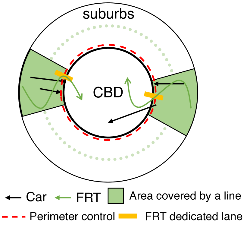
Figure 4: Model structure with perimeter control

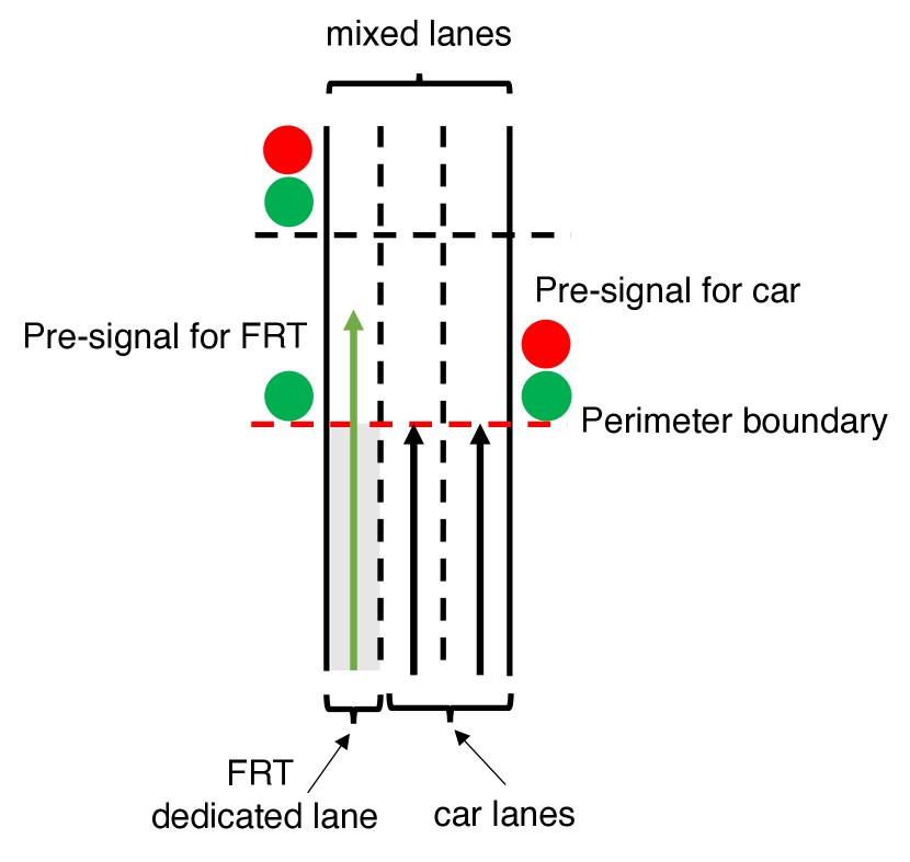
Figure 5: One example of the strategies of perimeter control with transit priority

4.1 Queuing dynamics at perimeter boundaries

Perimeter control aims to maintain the maximum throughput in the CBD zone (Geroliminis et al., 2012). From Eq. (3) we can derive the critical car accumulation, $\displaystyle n_{c}^{cr}$, where the throughput is maximized ($\displaystyle d\left(n_{c}(t)v_{c}(t)\right)/dn=0$).

$$\displaystyle n_{c}^{cr}=\frac{n_{j}^{\prime}}{2}$$ (40)

Eq. (40) indicates that the critical accumulation depends not only on car accumulation but also on FRT accumulation, since $\displaystyle n_{j}^{\prime}=n_{j}\left(1-\eta n_{F}^{c}/n_{j}\right)$. To prevent accumulation from exceeding the critical value, the inflow to the CBD zone is restricted at the perimeter boundary by gating or traffic signals once the accumulation reaches the critical density. The inflow rate to the CBD zone is set to the exit rate from the zone to maintain the critical accumulation, which means that the CBD traffic state is steady during perimeter control ($\displaystyle\dot{n_{c}}=0$ and $\displaystyle n_{c}(t)=n_{j}^{\prime}/2$ if $\displaystyle t_{s}^{p}\leq t<t_{e}^{p}$ where $\displaystyle t_{s}^{p}$ and $\displaystyle t_{e}^{p}$ are the perimeter control start and end times, respectively) . Thus, the inflow rate during perimeter control is determined from Eqs. (3)-(5) and (40) by

$$\displaystyle I_{c}^{p}=\frac{n_{j}^{\prime}v_{f}^{\prime}}{4L_{c}}$$ (41)

Therefore, the control scheme at time $\displaystyle t$ can be written by

$$\displaystyle I_{c}(t)=\begin{cases}I_{c}^{p}&\text{if }n_{c}(t)=\frac{n_{j}^{\prime}}{2}\\ A_{b}(t)&\text{if }n_{c}(t)<\frac{n_{j}^{\prime}}{2}\end{cases}$$ (42)

where $\displaystyle A_{b}(t)$ is the car arrival rate at the perimeter boundary at time $\displaystyle t$. If car accumulation is below the critical level, there is no restriction; all vehicles at the boundary can enter the CBD zone. Once accumulation reaches the critical accumulation, the inflow rate is restricted to $\displaystyle I_{c}^{p}$. This inflow rate can be regarded as the bottleneck capacity of the perimeter boundary. Thus, a queue will develop outward from the perimeter boundary if the demand exceeds the inflow rate $\displaystyle I_{c}^{p}$. We model the queuing dynamic as a point queue and assume first-arrived-first-in property. Therefore, the waiting time of a commuter who arrives at their destination at time $\displaystyle t$, $\displaystyle T_{b}(t)$, is

$$\displaystyle T_{b}(t)=\frac{q(t)}{I_{c}^{p}}$$ (43)

where $\displaystyle q(t)$ is the number of cars queued at the perimeter boundary when a commuter who arrives at their destination at time $\displaystyle t$ reaches the boundary.

4.2 Travel cost during perimeter control

Given the queue dynamics during perimeter control, the car travel cost incurred by a commuter who arrives at their destination at time $\displaystyle t$ is

$$\displaystyle C_{c}(t)=\begin{cases}\alpha T_{c}(t)+\beta\left(t^{*}-t\right)+F_{c}&\text{if }t<t_{s}^{p}\\ \alpha\left(\frac{L_{c}}{v_{f}^{\prime}/2}+T_{b}\left(t\right)\right)+\beta\left(t^{*}-t\right)+F_{c}&\text{if }t_{s}^{p}\leq t<t^{*}\\ \alpha\left(\frac{L_{c}}{v_{f}^{\prime}/2}+T_{b}\left(t\right)\right)+\gamma\left(t-t^{*}\right)+F_{c}&\text{if }t^{*}\leq t<t_{e}^{p}\\ \alpha T_{c}(t)+\gamma\left(t-t^{*}\right)+F_{c}&\text{if }t_{e}^{p}\leq t\end{cases}$$ (44)

Before and after perimeter control is implemented ( $\displaystyle t<t_{s}^{p}$ and $\displaystyle t_{e}^{p}\leq t$), the travel cost function is the same as Eq. (11). During perimeter control, the CBD travel time is given by $\displaystyle\frac{L_{c}}{v_{f}^{\prime}/2}$ since the trip completion rate is maintained at the maximum. In addition to the travel time cost , the cost of waiting at the perimeter boundary is incurred, as given by Eq. (43).

As FRT vehicles can pass the perimeter boundary freely by the dedicated lanes, there is no waiting time at the perimeter boundary. Therefore, the FRT travel cost incurred by a commuter who arrives at their destination at time $\displaystyle t$ is

$$\displaystyle C_{F}(t)=\begin{cases}\alpha T_{F}(t)+\beta\left(t^{*}-t\right)+\lambda O_{F}(t)+F_{F}&\text{if }t<t_{s}^{p}\\ \alpha\frac{L_{F}}{mv_{f}^{\prime}/2}+\beta\left(t^{*}-t\right)+\lambda O_{F}(t)+F_{F}&\text{if }t_{s}^{p}\leq t<t^{*}\\ \alpha\frac{L_{d}}{mv_{f}^{\prime}/2}+\gamma\left(t-t^{*}\right)+\lambda O_{F}(t)+F_{F}&\text{if }t^{*}\leq t<t_{e}^{p}\\ \alpha T_{F}(t)+\gamma\left(t-t^{*}\right)+\lambda O_{F}(t)+F_{F}&\text{if }t_{e}^{p}\leq t\end{cases}$$ (45)

5 Equilibrium under perimeter control

No commuter can reduce their travel cost by changing their departure time and transportation mode at equilibrium during perimeter control. Thus, the equilibrium conditions are

$$\displaystyle\begin{cases}C_{c}(t)=c^{*}_{p}&\text{if }n(t)>0\\ C_{c}(t)\geq c^{*}_{p}&\text{if }n(t)=0\\ \end{cases}\;\;\;\forall t\in\mathbb{R}$$ (46a)

$$\displaystyle\begin{cases}C_{F}(t)=c^{*}_{p}&\text{if }O_{F}(t)>0\\ C_{F}(t)\geq c^{*}_{p}&\text{if }O_{F}(t)=0\\ \end{cases}\;\;\;\forall t\in\mathbb{R}$$ (46b)

$$\displaystyle\begin{cases}n_{c}(t)=\frac{n_{j}^{\prime}}{2}&\text{if }q(t)>0\\ n_{c}(t)\leq\frac{n_{j}^{\prime}}{2}&\text{if }q(t)=0\end{cases}\;\;\;\forall t\in\mathbb{R}$$ (46c)

$$\displaystyle\int_{t\in\mathbb{R}}\frac{n_{c}(t)v_{c}(t)}{L_{c}}dt+\int_{t\in\mathbb{R}}\frac{O_{F}(t)n_{F}^{c}v_{F}(t)}{L_{F}}dt=N$$ (46d)

where $\displaystyle c^{*}_{p}$ is the equilibrium cost during perimeter control. Conditions (46a), (46b), and (46c) are the same as Conditions (15a), (15b) and (15c), respectively. Condition (46c) reflects the restriction of inflow to the CBD zone during perimeter control; car accumulation is at the critical accumulation if there is a queue at the perimeter boundary. Otherwise, car accumulation is lower than the critical level. Note that the difference in the conditions between user equilibrium and equilibrium under perimeter control is only Condition (46c). Moreover, dynamic user equilibrium under perimeter control is also based on Wardrop (1952)’s first principle.

5.1 Equilibrium properties

This study aims to analyse the cases where hypercongestion will occur at user equilibrium. Perimeter control can be implemented under the following condition.

Assumption 2.

$\displaystyle\theta>2$

From Condition (46a) and Eq. (44), the queue at the perimeter boundary during perimeter control has the same property as the standard bottleneck model.

Proposition 4.

Suppose Assumption 2. During perimeter control, a queue develops at the perimeter boundary, and its length increases toward the desired arrival time.

Proof.

Condition (46a) and Eq. (44) yield

$$\displaystyle\begin{cases}\alpha\frac{dT_{b}(t)}{dt}-\beta=0&\text{if }t_{s}^{p}\leq t<t^{*}\\ \\ \alpha\frac{dT_{b}(t)}{dt}+\gamma=0&\text{if }t^{*}\leq t<t_{e}^{p}\end{cases}$$ (47)

Combining this with Eq. (43), where $\displaystyle I_{c}(t)$ is constant (from Eq. (41)), we obtain

$$\displaystyle\begin{cases}\frac{dq(t)}{dt}=\frac{\beta}{\alpha}&\text{if }t_{s}^{p}\leq t<t^{*}\\ \frac{dq(t)}{dt}=-\frac{\gamma}{\alpha}&\text{if }t^{*}\leq t<t_{e}^{p}\end{cases}$$ (48)

which completes the proof. ∎

This proposition indicates that some commuters prefer to wait at the perimeter boundary rather than change their departure times or transportation modes. Since the arrival rate in the CBD is maintained at its maximum during perimeter control and the schedule delay cost decreases toward the desired arrival time, commuters can travel at the equilibrium cost, even if they have to wait at the perimeter boundary. This mechanism is completely the same as that of the standard bottleneck model (Arnott et al., 1993).

We define $\displaystyle\theta_{p}\equiv\frac{(c_{p}^{*}-F_{c})v_{f}^{\prime}}{\alpha L_{c}}$. Although the effectiveness of the combination of perimeter control and transit priority has been reported (e.g., Haitao et al. (2019)), we present the following proposition.

Proposition 5.

Suppose Assumption 2. The equilibrium with perimeter control has the following properties.

1. If $\displaystyle\Delta F\geq 2\alpha\Delta T_{f}$, then FRT is used from the beginning to the end during the FRT rush hour and the number of FRT passengers increases toward the desired arrival time during perimeter control.

2. If $\displaystyle\Delta F<2\alpha\Delta T_{f}$ and $\displaystyle\theta_{p}>\frac{2\alpha T_{f}^{F}-\Delta F}{\alpha T_{f}^{c}}$, then FRT is used; however, there will be a time window wherein FRT is not used during perimeter control. Additionally, the number of FRT passengers increases toward the desired arrival time during perimeter control.

3. If $\displaystyle\theta_{p}\leq\frac{2\alpha T_{f}^{F}-\Delta F}{\alpha T_{f}^{c}}$, then FRT is not used during perimeter control.

Proof.

Condition (46a) yields Eq. (16) for car accumulation before and after perimeter control. Thus, the start and end times of perimeter control ($\displaystyle t_{s}^{p}$ and $\displaystyle t_{e}^{p}$, respectively; $\displaystyle n_{c}(t_{s}^{p})=n(t_{e}^{p})=n_{j}^{\prime}/2$) are

$$\displaystyle t_{s}^{p}-t_{s}^{c}=\frac{\alpha T_{f}^{c}}{\beta}$$ (49)

$$\displaystyle t_{e}^{c}-t_{e}^{p}=\frac{\alpha T_{f}^{c}}{\gamma}$$ (50)

Eqs. (23) and (24) give the time window when FRT is not used during the FRT rush hour. When the start of perimeter control is earlier than the start of the above time window (i.e., $\displaystyle t_{ee}^{F}\geq t_{s}^{p}$ ), combining Eq. (49) with Eq. (23) gives

$$\displaystyle\Delta F\geq 2\alpha\Delta T_{f}$$ (51)

Note that $\displaystyle 2\alpha\Delta T_{f}$ is the difference of the car and FRT travel time costs at the critical car accumulation. According to Eq. (45) and Condition (46b), $\displaystyle\dot{O_{F}}(t)=\beta/\lambda$ if $\displaystyle t_{s}^{p}\leq t\leq t^{*}$ and $\displaystyle\dot{O_{F}}(t)=-\gamma/\lambda$ if $\displaystyle t^{*}<t\leq t_{e}^{p}$. Thus, the number of FRT passengers increases toward the desired arrival time during perimeter control. Therefore, if $\displaystyle\Delta F\geq 2\alpha\Delta T_{f}$, FRT is used throughout the FRT rush hour, and the number of FRT passengers increases toward the desired arrival time during perimeter control.

Let $\displaystyle[t_{sp}^{F},t_{ep}^{F}]$ be the time window between the start and end times when FRT is used during perimeter control. If $\displaystyle t_{sp}^{F}<t^{*}$ (i.e., $\displaystyle t_{ep}^{F}>t^{*}$), there is a time window when FRT is used during perimeter control. Since $\displaystyle O_{F}(t_{sp}^{F})=0$, Eq. (45) yields

$$\displaystyle\alpha\frac{L_{F}}{mv_{f}^{\prime}/2}+\beta\left(t^{*}-t_{sp}^{F}\right)+F_{F}=c_{p}^{*}$$ (52)

From Eq. (52), $\displaystyle t_{sp}^{F}<t^{*}$ can be rewritten as

$$\displaystyle\theta_{p}>\frac{2\alpha T_{f}^{F}-\Delta F}{\alpha T_{f}^{c}}$$ (53)

Therefore, even when $\displaystyle\Delta F<2\alpha\Delta T_{f}$, there is a time window when FRT is used during perimeter control if $\displaystyle\theta_{p}>\frac{2\alpha T_{f}^{F}-\Delta F}{\alpha T_{f}^{c}}$. Otherwise, FRT is not used during perimeter control.

∎

Proposition 5.1 indicates that FRT is used from the beginning to the end during the FRT rush hour if the fixed cost difference ($\displaystyle\Delta F$) is larger than the travel time cost difference during perimeter control at the critical car accumulation ($\displaystyle 2\alpha\Delta T_{f}$). Moreover, the average number of passengers per FRT vehicle begins to increase toward the desired arrival time once perimeter control starts ($\displaystyle t>t_{s}^{p}$), as depicted in Fig. 6. Since the FRT travel time cost is constant during perimeter control (Eq. (45)), $\displaystyle\dot{O_{F}}(t)=\beta/\lambda$ for earliness, which is the same as the time evolution of $\displaystyle O_{F}(t)$ before the car rush hour starts. A trade-off exists between the schedule delay and discomfort costs. In the same way, $\displaystyle\dot{O_{F}}(t)=-\gamma/\lambda$ for lateness. Thus, there is no time interval when FRT is not used during the FRT rush hour.

From Proposition 5.2, FRT is used if $\displaystyle\Delta F<2\alpha\Delta T_{f}$ and the FRT free-flow travel time cost ($\displaystyle T_{f}^{F}$) and fixed cost ($\displaystyle F_{F}$) are relatively low compared to the other costs (i.e., $\displaystyle\theta_{p}>(2\alpha T_{f}^{F}-\Delta F)/(\alpha T_{f}^{c})$). However, there will be a time window wherein FRT is not used during perimeter control and the FRT rush hour. As depicted in Fig. 7, the number of FRT commuters becomes zero before perimeter control starts. Since the travel time cost is constant during perimeter control, the FRT travel cost decreases with a decrease in the schedule delay cost toward the desired arrival time, and FRT is used. Once the use of FRT begins, the average number of passengers per FRT vehicle increases toward the desired arrival time, as in Proposition 5.1. Since providing transit priority is not effective during the time window wherein FRT is not used, it limits the capacity of the perimeter boundary during this period. Therefore, additional incentives that reduce the FRT travel cost, such as subsidy so that $\displaystyle\Delta F\geq 2\alpha\Delta T_{f}$ is satisfied, may be required to promote the use of FRT from the beginning to the end of perimeter control.

Although prioritization of transit at the perimeter boundaries is a better strategy than unimodal perimeter control in terms of passenger mobility (Haitao et al., 2019), Proposition 5.3 states that this is false if $\displaystyle\theta_{p}\leq(2\alpha T_{f}^{F}-\Delta F)/(\alpha T_{f}^{c})$, and FRT is not used during perimeter control. In this case, the FRT travel cost is higher than the car travel cost during perimeter control despite that FRT vehicles do not queue at the perimeter boundary. Hence, the bimodal transportation system is not fully utilized. As the vacant FRT vehicles circulate in the CBD zones and are prioritized at the perimeter boundary, these vehicles and transit priority (e.g., dedicated lanes) waste urban spaces around the peak of the rush hour. Ultimately, the effect of the strategy is the same as that of unimodal perimeter control in terms of passenger flow. To promote the use of FRT during perimeter control, additional incentives that satisfy at least $\displaystyle\theta_{p}>(2\alpha T_{f}^{F}-\Delta F)/(\alpha T_{f}^{c})$ are required.

Figure 6: Illustration of Proposition 5.1

Figure 7: Illustration of Proposition 5.2

5.2 Equilibrium cost

We derive the equilibrium cost when FRT is used from the beginning to the end during perimeter control ( $\displaystyle\Delta F>2\alpha\Delta T_{f}$). The number of commuters who take FRT before and after the car rush hour is the same as that in the case with user equilibrium.

$$\displaystyle N_{F}^{oc} \displaystyle= \displaystyle\frac{n_{F}^{c}}{2\lambda}\frac{1}{T_{f}^{F}}\left(\frac{1}{\beta}+\frac{1}{\gamma}\right)\left(\Delta F-\alpha\Delta T_{f}\right)^{2}$$ (54)

The number of commuters who take FRT during the car rush hour outside the perimeter control period ($\displaystyle t\in[t_{s}^{c},t_{s}^{p})$ and $\displaystyle t\in[t_{e}^{p},t_{e}^{c})$ ) is

$$\displaystyle N_{F}^{op} \displaystyle= \displaystyle\int_{t_{s}^{c}}^{t_{s}^{p}}\frac{O_{F}(s)n_{F}^{c}v_{F}(s)}{L_{F}}ds+\int_{t_{e}^{p}}^{t_{e}^{c}}\frac{O_{F}(s)n_{F}^{c}v_{F}(s)}{L_{F}}ds$$ (55)

$$\displaystyle= \displaystyle n_{F}^{c}\frac{\alpha}{\lambda}\frac{T_{f}^{c}}{T_{f}^{F}}\left(\frac{1}{\beta}+\frac{1}{\gamma}\right)\left(\Delta F\ln 2-\alpha\Delta T_{f}\right)$$

When perimeter control starts, the average number of passengers per FRT vehicle is computed using Eqs. (44) and (45).

$$\displaystyle O_{F}(t_{s}^{p})=\frac{1}{\lambda}\left(\Delta F-2\alpha\Delta T_{f}\right)$$ (56)

Furthermore, we obtain $\displaystyle\dot{O_{F}}(t)=\beta/\lambda$, $\displaystyle t\in[t_{s}^{p},t^{*})$ from Eq. (45). Thus, the time evolution of the average number of passengers per FRT vehicle is

$$\displaystyle O_{F}(t)=\frac{1}{\lambda}\left(\Delta F-2\alpha\Delta T_{f}+\beta(t-t_{s}^{p})\right)\;\;\;\text{if}\;\;\;t_{s}^{p}\leq t\leq t^{*}$$ (57)

This can be obtained for lateness in the same manner. Thus,

$$\displaystyle O_{F}(t)=\begin{cases}\frac{1}{\lambda}\left(\Delta F-2\alpha\Delta T_{f}+\beta(t-t_{s}^{p})\right)\;\;\;\text{if}\;\;\;t_{s}^{p}\leq t\leq t^{*}\\ \frac{1}{\lambda}\left(\Delta F-2\alpha\Delta T_{f}+\gamma(t_{e}^{p}-t)\right)\;\;\;\text{if}\;\;\;t^{*}<t\leq t_{e}^{p}\end{cases}$$ (58)

The total number of FRT commuters who arrive at their destinations during perimeter control is

$$\displaystyle N_{F}^{p}=\int_{t_{s}^{p}}^{t^{*}}\frac{O_{F}(s)n_{F}^{c}mv_{f}^{\prime}/2}{L_{F}}ds+\int_{t^{*}}^{t_{e}^{p}}\frac{O_{F}(s)n_{F}^{c}mv_{f}^{\prime}/2}{L_{F}}ds$$ (59)

We combine Eqs. (58) and (59) and obtain

$$\displaystyle N_{F}^{p}=\frac{n_{F}^{c}}{2T_{f}^{F}}\frac{1}{\lambda}\left(\frac{1}{\beta}+\frac{1}{\gamma}\right)\left(c_{p}^{*}-2\alpha T_{f}^{c}-F_{c}\right)\left(\Delta F-2\alpha\Delta T_{f}+\frac{1}{2}\left(c_{p}^{*}-2\alpha T_{f}^{c}-F_{c}\right)\right)$$ (60)

Since $\displaystyle c_{p}^{*}=2\alpha T_{f}^{c}+\beta\left(t^{*}-t_{s}^{p}\right)+F_{c}=2\alpha T_{f}^{c}+\gamma\left(t_{e}^{p}-t^{*}\right)+F_{c}$, substituting this into Eq.(60), we obtain:

$$\displaystyle N_{F}^{p}=\frac{n_{F}^{c}}{2}\frac{\alpha}{\lambda}\frac{T_{f}^{c}}{T_{f}^{F}}\left(\frac{1}{\beta}+\frac{1}{\gamma}\right)\left(\theta^{p}-2\right)\left(\Delta F-2\alpha\Delta T_{f}+\frac{\alpha T_{f}^{c}}{2}\left(\theta^{p}-2\right)\right)$$ (61)

where $\displaystyle\theta^{p}\equiv\frac{(c_{p}^{*}-F_{c})v_{f}^{\prime}}{\alpha L_{c}}$.

As the car trip completion rate is maintained at the maximum ($\displaystyle G_{c}(t)=n_{j}^{\prime}v_{f}^{\prime}/4L_{c}$, $\displaystyle t\in[t_{s}^{p},t_{e}^{p})$), the number of car commuters who arrive at their destination during perimeter control is

$$\displaystyle N_{c}^{p}=\frac{n_{j}^{\prime}v_{f}^{\prime}}{4L_{c}}(t_{e}^{p}-t_{s}^{p})$$ (62)

Since $\displaystyle c_{p}^{*}=2\alpha T_{f}^{c}+\beta\left(t^{*}-t_{s}^{p}\right)+F_{c}=2\alpha T_{f}^{c}+\gamma\left(t_{e}^{p}-t^{*}\right)+F_{c}$, substituting it into Eq.(62), we have:

$$\displaystyle N_{c}^{p}=\frac{\alpha n_{j}^{\prime}}{4}\left(\frac{1}{\beta}+\frac{1}{\gamma}\right)\left(\theta^{p}-2\right)$$ (63)

The number of car commuters who arrive at their destinations before and after perimeter control is computed using Eqs. (3), (16), (49), and (50) by

$$\displaystyle N_{c}^{op} \displaystyle= \displaystyle\int_{t_{s}^{c}}^{t_{s}^{p}}\frac{n_{c}(s)v_{c}(s)}{L_{c}}ds+\int_{t_{e}^{p}}^{t_{e}^{c}}\frac{n_{c}(s)v_{c}(s)}{L_{c}}ds$$ (64)

$$\displaystyle= \displaystyle n_{j}^{\prime}\left(\frac{\alpha}{\beta}+\frac{\alpha}{\gamma}\right)\left(\ln 2-\frac{1}{2}\right)$$

We combine Eqs. (54), (55), (61), (63), and (64), and the total number of commuters is

$$\displaystyle N= \displaystyle\left(\frac{1}{\beta}+\frac{1}{\gamma}\right)\left[\frac{\alpha n_{j}^{\prime}}{4}\left(\theta^{p}-2\right)+\alpha n_{j}^{\prime}\left(\ln 2-\frac{1}{2}\right)+\right.$$ (65)

$$\displaystyle\left.\frac{n_{F}^{c}}{\lambda}\frac{1}{T_{f}^{F}}\left(\frac{\alpha T_{f}^{c}}{2}\left(\theta^{p}-2\right)\left(\Delta F-2\alpha\Delta T_{f}+\frac{\alpha T_{f}^{c}}{2}\left(\theta^{p}-2\right)\right)+\frac{1}{2}\left(\Delta F-\alpha\Delta T_{f}\right)^{2}+\alpha T_{f}^{c}\left(\Delta F\ln 2-\alpha\Delta T_{f}\right)\right)\right]$$

Given that $\displaystyle\theta^{p}\equiv\frac{(c_{p}^{*}-F_{c})v_{f}^{\prime}}{\alpha L_{c}}$, this can also be solved numerically with respect to the equilibrium cost $\displaystyle c_{p}^{*}$.

We derive the equilibrium cost for the case where FRT is used, but there will a time window wherein FRT is not used during perimeter control ($\displaystyle\Delta F\leq 2\alpha\Delta T_{f}$ and $\displaystyle\theta_{p}>\frac{2\alpha T_{f}^{F}-\Delta F}{\alpha T_{f}^{c}}$). Since $\displaystyle O_{F}(t_{sp}^{F})=O_{F}(t_{ep}^{F})=0$, the start and end times when FRT is used during perimeter control are given from Eq. (45) by

$$\displaystyle t^{*}-t_{sp}^{F}=\frac{1}{\beta}\left(c^{*}_{p}-2\alpha T_{f}^{F}-F_{F}\right)$$ (66)

$$\displaystyle t_{ep}^{F}-t^{*}=\frac{1}{\gamma}\left(c^{*}_{p}-2\alpha T_{f}^{F}-F_{F}\right)$$ (67)

Since $\displaystyle\dot{O_{F}}(t)=\beta/\lambda$, $\displaystyle t\in[t_{sp}^{F},t^{*})$ and $\displaystyle\dot{O_{F}}(t)=-\gamma/\lambda$, $\displaystyle t\in[t^{*},t_{ep}^{F})$ from Eq. (45), the total number of FRT commuters who arrive at their destinations during perimeter control is

$$\displaystyle N_{F}^{p} \displaystyle= \displaystyle\int_{t_{sp}^{F}}^{t^{*}}\frac{O_{F}(s)n_{F}^{c}mv_{f}^{\prime}/2}{L_{F}}ds+\int_{t^{*}}^{t_{ep}^{F}}\frac{O_{F}(s)n_{F}^{c}mv_{f}^{\prime}/2}{L_{F}}ds$$ (68)

$$\displaystyle= \displaystyle\frac{n_{F}^{c}}{2\lambda}\frac{\left(\alpha T_{f}^{c}\right)^{2}}{2T_{f}^{F}}\left(\frac{1}{\beta}+\frac{1}{\gamma}\right)\left(\theta^{p}-\frac{2\alpha T_{f}^{F}-\Delta F}{\alpha T_{f}^{c}}\right)^{2}$$

The number of FRT commuters before and after perimeter control is given by Eq. (35). As the total number of car commuters is given by the sum of Eqs. (62) and (63), we combine Eqs. (35),(62), (63), and (68), and the total number of commuters satisfies

$$\displaystyle N \displaystyle= \displaystyle\left(\frac{1}{\beta}+\frac{1}{\gamma}\right)\left[\frac{\alpha n_{j}^{\prime}}{4}\left(\theta^{p}-2\right)+\alpha n_{j}^{\prime}\left(\ln 2-\frac{1}{2}\right)+\right.$$ (69)

$$\displaystyle\left.\frac{n_{F}^{c}}{\lambda}\frac{1}{T_{f}^{F}}\left(\frac{\left(\alpha T_{f}^{c}\right)^{2}}{4}\left(\theta_{p}-\frac{2\alpha T_{f}^{F}-\Delta F}{\alpha T_{f}^{c}}\right)^{2}+\frac{1}{2}\left(\Delta F-\alpha\Delta T_{f}\right)^{2}+\alpha T_{f}^{c}\left(\Delta F\ln\frac{\Delta F}{\alpha\Delta T_{f}}-\left(\Delta F-\alpha\Delta T_{f}\right)\right)\right)\right]$$

Given that $\displaystyle\theta^{p}\equiv\frac{(c_{p}^{*}-F_{c})v_{f}^{\prime}}{\alpha L_{c}}$, this can also be solved numerically with respect to the equilibrium cost $\displaystyle c_{p}^{*}$.

Even if Assumption 1 is not satisfied, FRT is used during perimeter control provided $\displaystyle\theta_{p}>\frac{2\alpha T_{f}^{F}-\Delta F}{\alpha T_{f}^{c}}$. In this case, FRT is used only during perimeter control. The number of FRT commuters is given by Eq. (68). Thus, the total number of commuters is

$$\displaystyle N \displaystyle= \displaystyle\left(\frac{1}{\beta}+\frac{1}{\gamma}\right)\left[\frac{\alpha n_{j}^{\prime}}{4}\left(\theta^{p}-2\right)+\alpha n_{j}^{\prime}\left(\ln 2-\frac{1}{2}\right)+\frac{n_{F}^{c}}{\lambda}\frac{1}{T_{f}^{F}}\frac{\left(\alpha T_{f}^{c}\right)^{2}}{4}\left(\theta_{p}-\frac{2\alpha T_{f}^{F}-\Delta F}{\alpha T_{f}^{c}}\right)^{2}\right]$$ (70)

where $\displaystyle\theta^{p}\equiv\frac{(c_{p}^{*}-F_{c})v_{f}^{\prime}}{\alpha L_{c}}$. This can also be solve numerically.

Next, we derive the equilibrium cost for the case where FRT is not used during perimeter control. If $\displaystyle\theta_{p}\leq\frac{2\alpha T_{f}^{F}-\Delta F}{\alpha T_{f}^{c}}$, then perimeter control is never implemented if Assumption 1 holds (See Appendix B for the proof ). Thus, when perimeter control is implemented, Assumption 1 is not satisfied, indicating that the total number of commuters is equal to the number of car commuters since FRT is never used, and is given by

$$\displaystyle N \displaystyle= \displaystyle\left(\frac{1}{\beta}+\frac{1}{\gamma}\right)\left(\frac{\alpha n_{j}^{\prime}}{4}\left(\theta^{p}-2\right)+\alpha n_{j}^{\prime}\left(\ln 2-\frac{1}{2}\right)\right)$$ (71)

As with the user equilibrium without perimeter control, the equilibrium cost during perimeter control has the following property.

Proposition 6.

The equilibrium cost during perimeter control is uniquely determined, regardless of whether or not FRT is used during perimeter control.

Proof.

See Appendix C. ∎

Although the equilibrium cost is uniquely determined, the impacts of certain parameters on the equilibrium cost and mode share are unclear. For example, Eqs. (65), (69), (70), and (71) show that the number of FRT vehicles may increase and decrease the equilibrium cost. Therefore, the properties of equilibrium with and without perimeter control, such as its cost and the role of certain parameters (e.g., the number of FRT vehicles), are investigated through numerical examples in the next section.

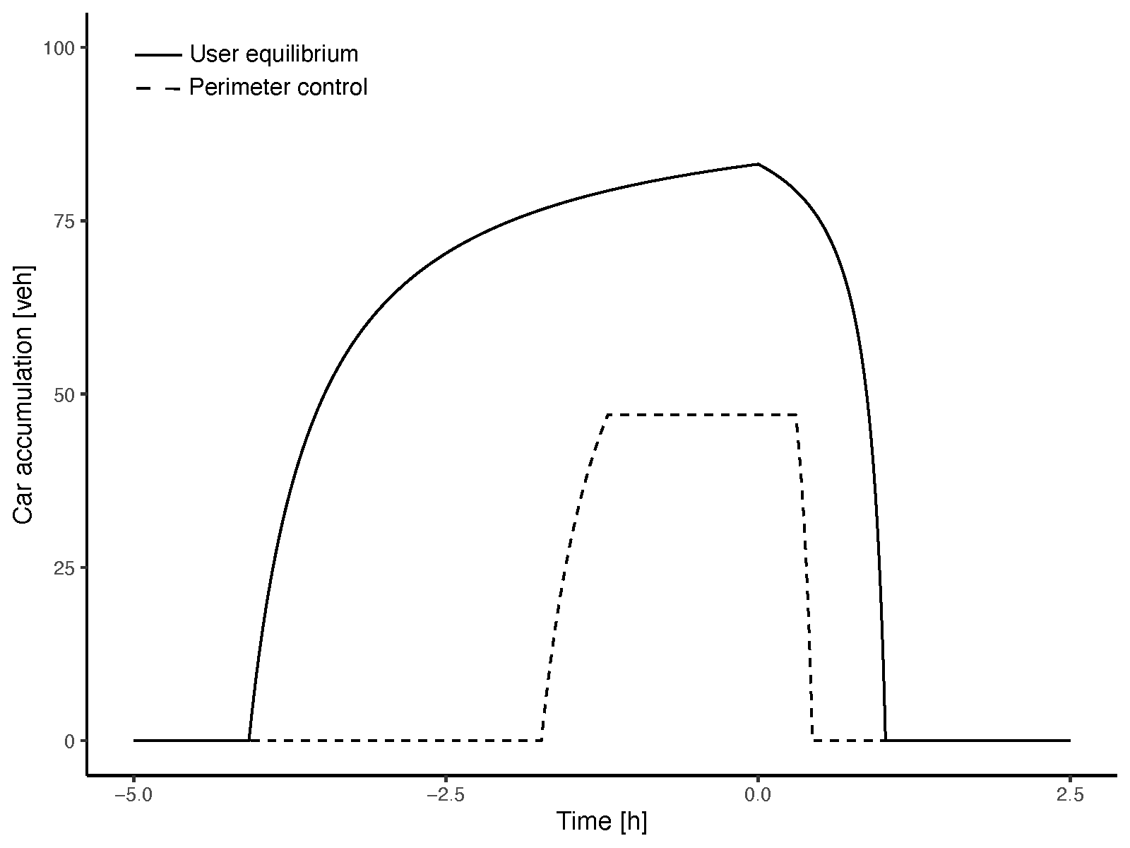
(a) Case I

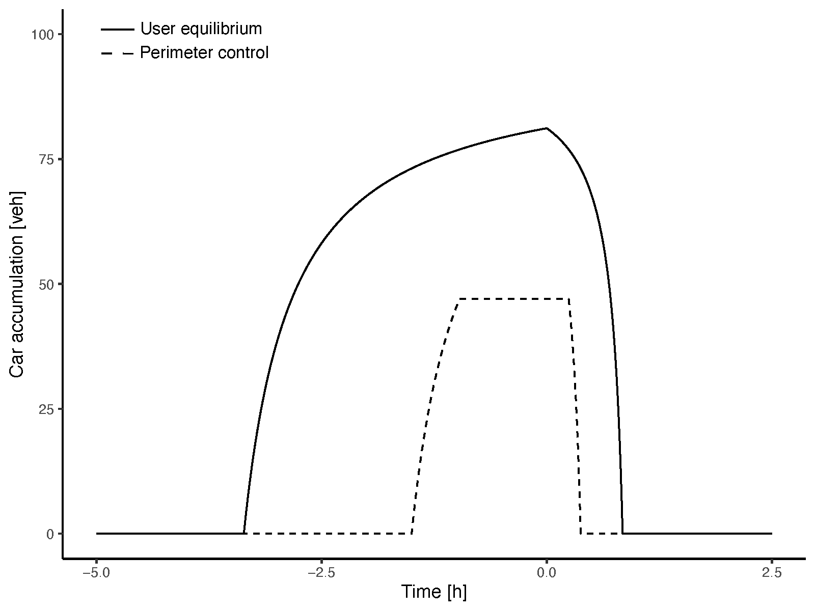
(b) Case II

Figure 8: Car accumulation in the CBD zone

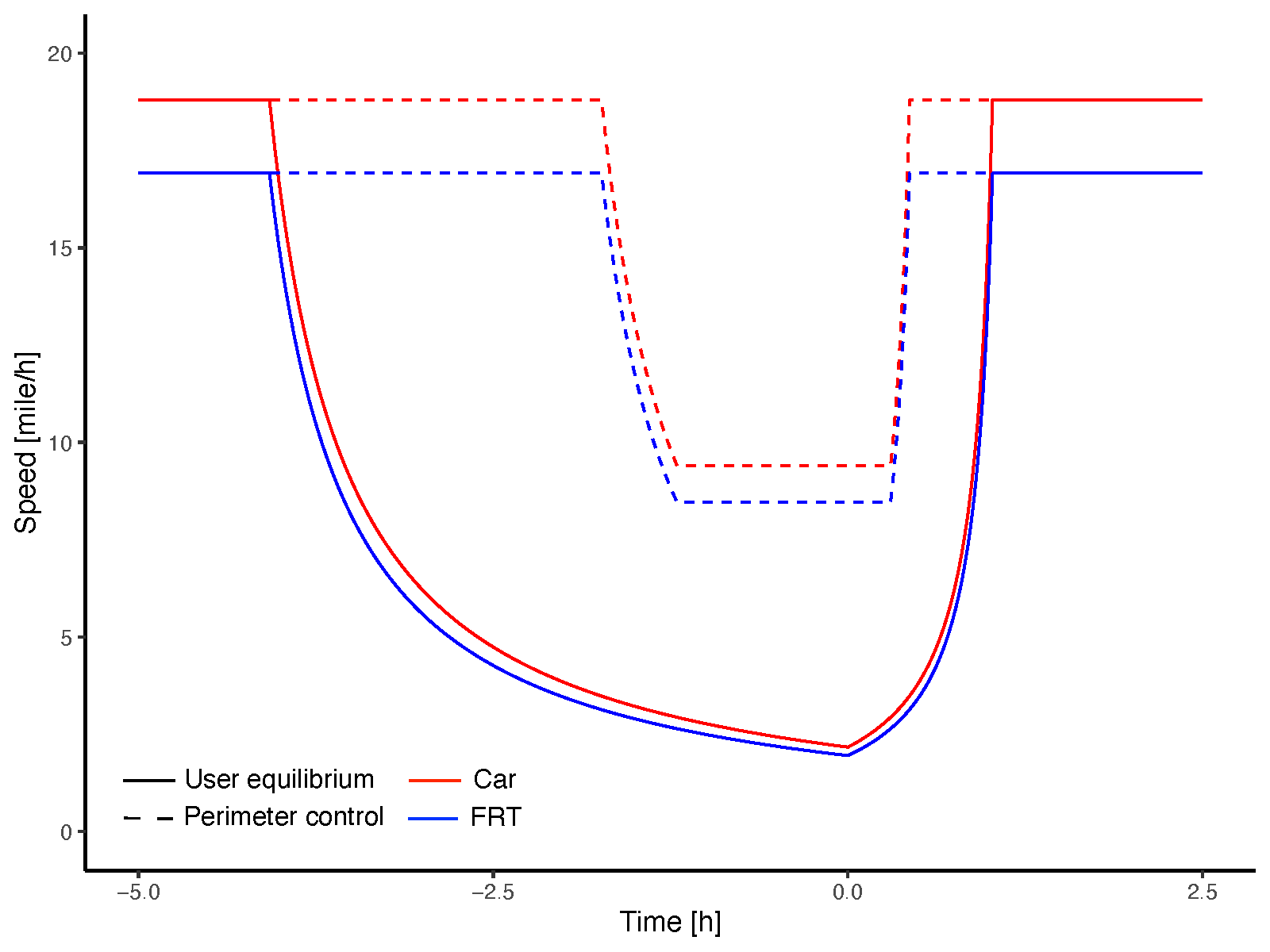
(a) Case I

(b) Case II

Figure 9: Speed in the CBD zone

6 Numerical examples

We numerically investigate the equilibrium patterns of the mixed bimodal bathtub model. The parameters are as follows: $\displaystyle v_{f}=20$ [mile/h], $\displaystyle\eta=1.2$, $\displaystyle n_{F}^{c}=5$ [veh], $\displaystyle n_{j}=100$ [veh], $\displaystyle m=0.9$, $\displaystyle\alpha,\beta,\gamma=20,10,40$ [$/h], $\displaystyle F_{c}=5$ [$], $\displaystyle L_{c},L_{F}=5,6$ [mile], $\displaystyle N=300$ [pax], $\displaystyle\lambda=0.4$ [$/pax] and $\displaystyle t^{*}=0$. Some of the parameters are taken from Arnott (2013). Note that as we set the desired arrival time to zero, the negative time indicates the time before the desired arrival time (i.e., earliness), and the positive time indicates the time after the desired arrival time (i.e., lateness). We compare the equilibrium patterns of two cases: with FRT partial use (Case I) and with FRT use (Case II) during perimeter control. Thus, in addition to above parameters, we set the FRT fixed cost to $\displaystyle F_{F}=2$ [$] for Case I and to $\displaystyle F_{d}=1$ [$] for case II.

Car accumulation between Cases I and II is compared in Fig. 9. In both cases, a similar evolution of car accumulation is obtained; however, because of the higher FRT fixed cost for Case I, more commuters use their cars, which leads to a longer rush hour. At user equilibrium, hypercongestion occurs (above $\displaystyle n_{j}^{\prime}/2=47$ [veh]), and the highest accumulation is reached at the desired arrival time. These results are consistent with those in the literature on unimodal bathtub models (e.g., Small and Chu (2003); Geroliminis and Levinson (2009); Arnott (2013)).

During perimeter control, critical accumulation is maintained around the desired arrival time. In both cases, the rush hour is shortened during perimeter control. This is because the traffic condition in the CBD zone never reaches hypercongestion, and the arrival rate is maintained at the maximum during perimeter control. Thus, more commuters can arrive at their destinations near the desired arrival time. These features are visible from the speed profiles in Fig. 9 as well.

As depicted in Figs. 11 and 11, traffic becomes hypercongested once the maximum car arrival rate is reached at user equilibrium, hence the car arrival rate decreases toward the desired arrival time. When perimeter control is implemented, the car arrival rate is maintained at the maximum for both cases. The FRT passenger arrival rate and the average number of passengers per FRT vehicle differ between the two cases. In Case I, there is a time window wherein FRT is not used during the FRT rush hour regardless of perimeter control. During perimeter control, FRT is used again and the arrival rate increases toward the desired arrival time, as verified in Proposition 5.2. Even though the FRT vehicular arrival rate is constant during perimeter control, the passenger arrival rate increases because the average number of passengers per FRT vehicle increases, which is depicted in Fig. 11 (a) and verified in Proposition 5.2. At user equilibrium without perimeter control in Case II, the number of FRT commuters is higher than that in Case I due to the lower FRT fixed cost, but its evolution pattern is the same as that in Case I as depicted in Fig. 11 (b). It is also shown that at equilibrium with perimeter control, FRT is used from the beginning to the end during the FRT rush hour. Once perimeter control starts, the arrival rate begins to increase because of the increase in the average number of passengers per FRT vehicle, which is depicted in Fig. 11 (b) and verified in Proposition 5.1.

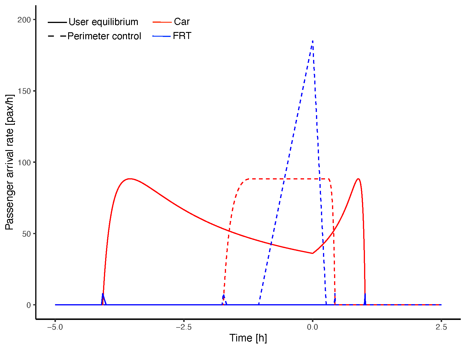
(a) Case I

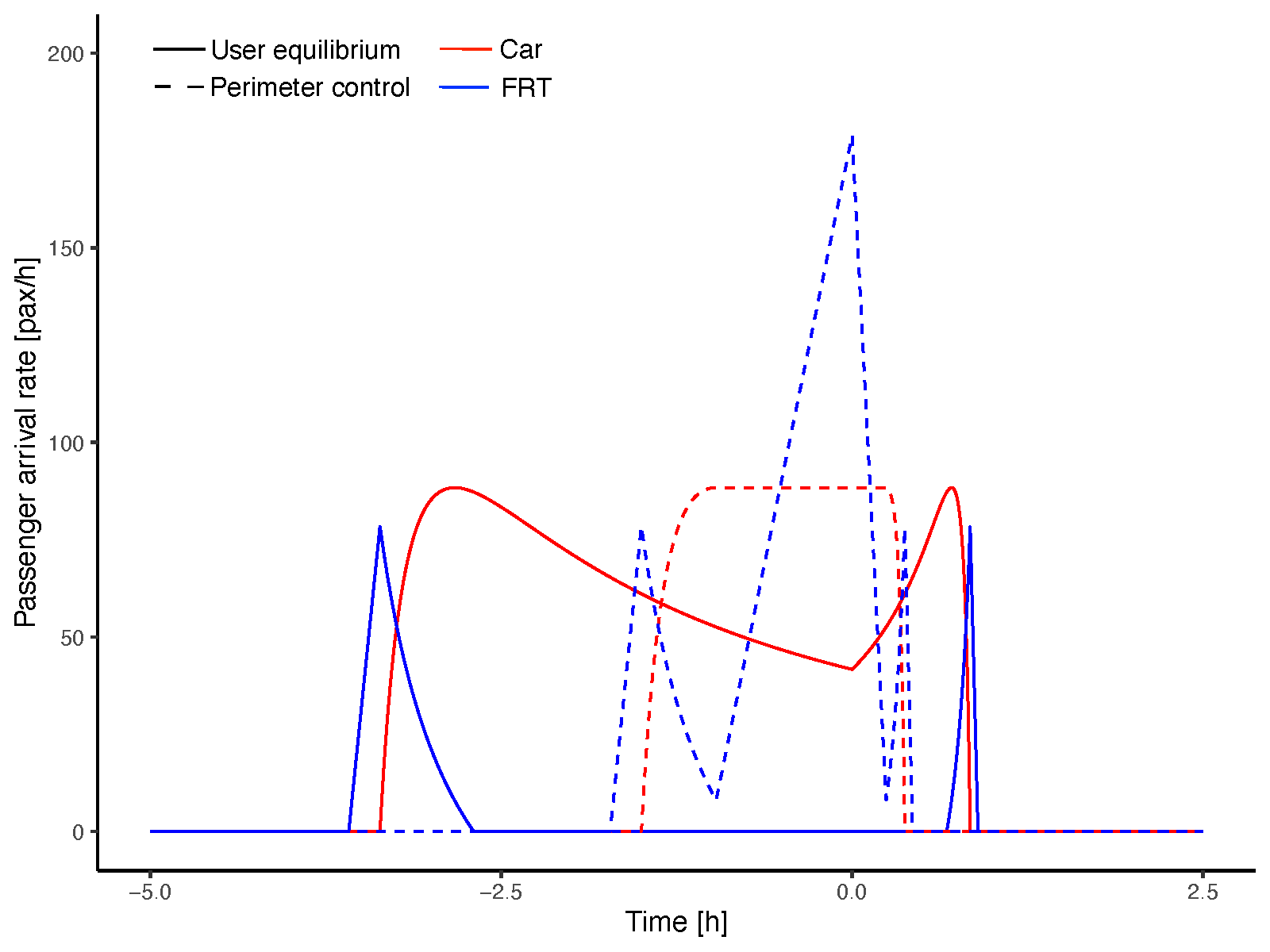
(b) Case II

Figure 10: Passenger arrival rate at their destination

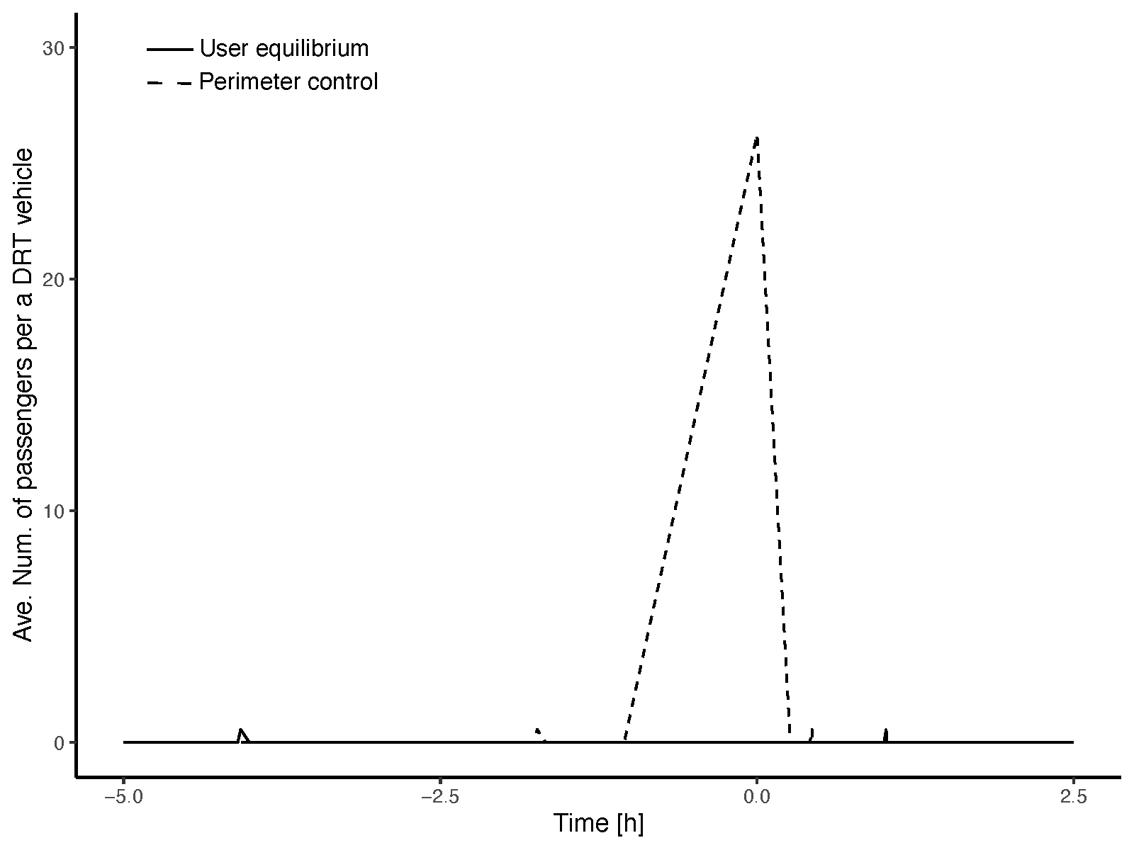
(a) Case I

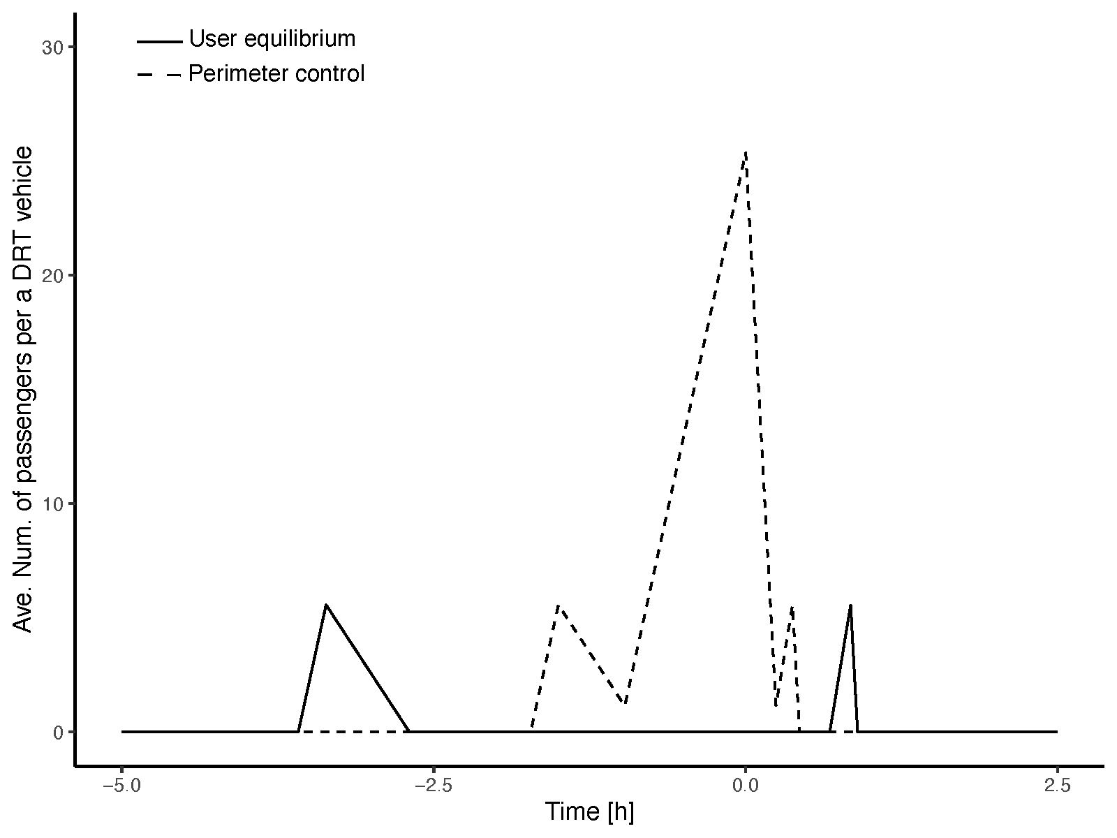
(b) Case II

Figure 11: Average number of passengers per a FRT vehicle

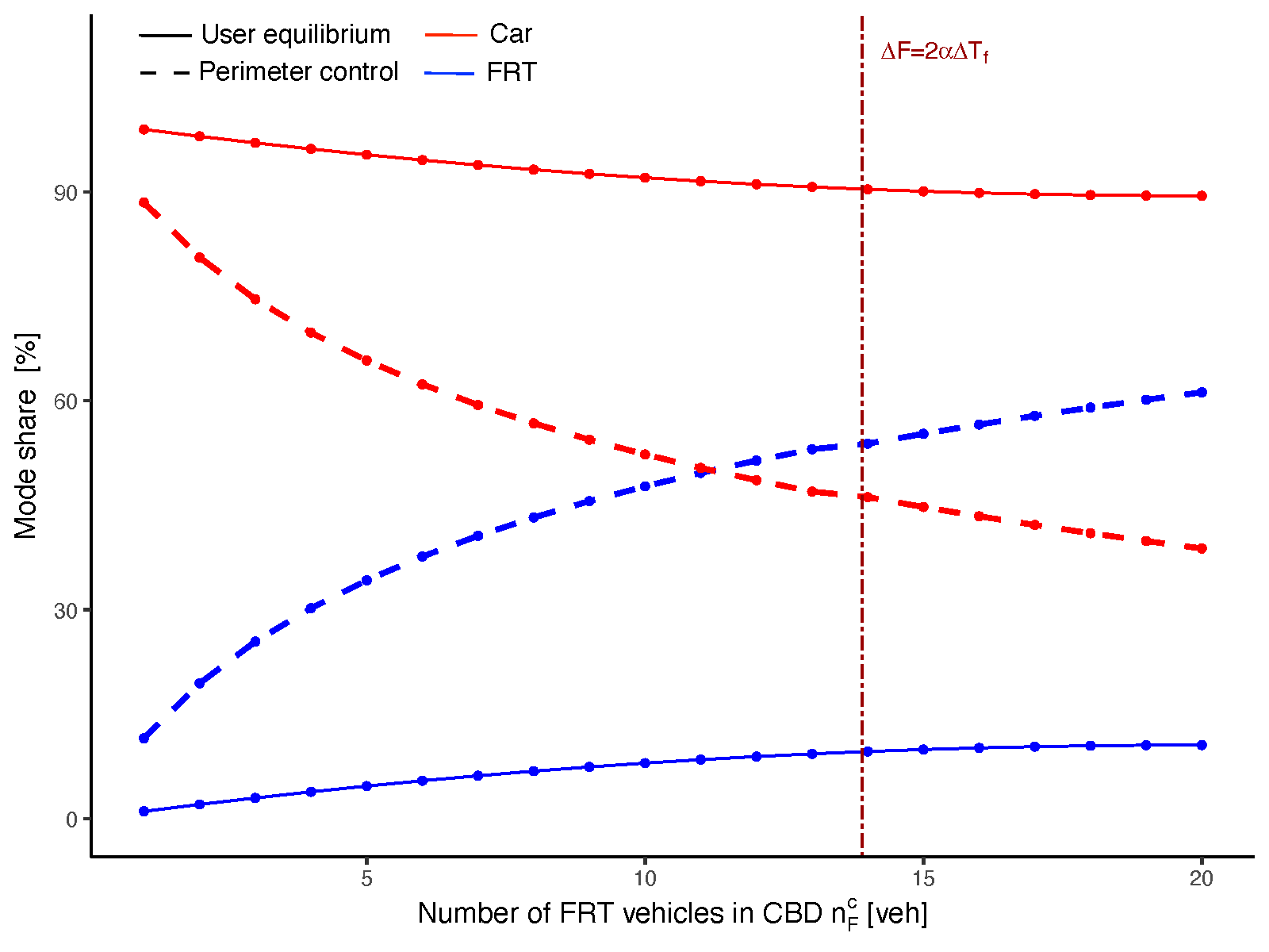
(a) Mode share

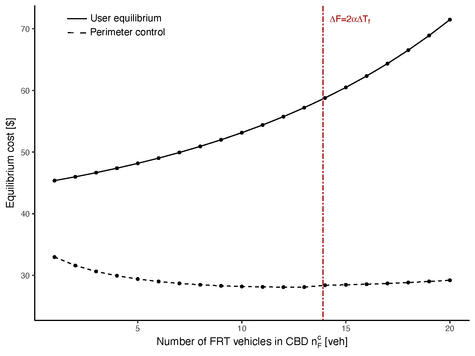
(b) Equilibrium cost

Figure 12: Sensitivity analysis to number of FRT vehicles (the vertical dotted line represents the number of FRT vehicles; $\displaystyle\Delta F=2\alpha\Delta T_{f}$ )

Table 1: Sensitivity analysis to number of FRT vehicles

	User equilibrium		Perimeter control
$\displaystyle n_{F}^{c}$	$\displaystyle c^{*}$	FRT mode share [%]	$\displaystyle c_{p}^{*}$	FRT mode share [%]	$\displaystyle\frac{c_{p}^{*}}{c^{*}}$
1	45.4	1.0	33.0	11.5	0.73
5	48.2	4.7	29.4	34.2	0.61
10	53.1	8.0	28.2	47.7	0.53
15	60.5	9.9	28.5	55.3	0.47
20	71.5	10.6	29.2	61.2	0.41

6.1 Sensitivity analysis with respect to number of FRT vehicles

We then analyze the sensitivity with respect to the number of FRT vehicles in the CBD zone, $\displaystyle n_{F}^{c}$, as shown in Fig. 12 and Table. 1. The vertical dotted line in Fig. 12 corresponds to the cost which yields $\displaystyle\Delta F=2\alpha\Delta T_{f}$; $\displaystyle 13<n_{F}^{c}<14$. We find that, as more FRT vehicles are operated, more passengers take FRT. We also find from Fig. 12 (b) and Table. 1 that the increase in the number of FRT vehicles simply increases the user equilibrium cost, whereas the increase in the number of FRT vehicles decreases the equilibrium cost under perimeter control when a few FRT vehicles are operated; however it increases the cost if too many FRT vehicles are operated. This is because the increase in the number of FRT vehicles not only alleviates the discomfor (discomfort effect hereafter), but also decreases the network capacity (network capacity effect hereafter). The network capacity effect is larger in the presence of hypercongestion and result in an increase in the user equilibrium cost. Conversely, as hypercongestion does not occur under perimeter control, the network capacity effect is relatively smaller. Therefore, the discomfort effect decreases the equilibrium cost until a certain number of vehicles is reached ($\displaystyle 13$ [veh] in this example). If the number of FRT vehicles exceeds this threshold, then the network capacity becomes larger and causes an increase in the equilibrium cost. This implies that operating many FRT vehicles to promote mode shift from cars during perimeter control may increase the equilibrium cost.

To investigate the impact of perimeter control, we estimate the ratio of the equilibrium cost with perimeter control to the user equilibrium cost as shown in the last column of Table. 1. We find that the impact of perimeter control increases with the number of FRT vehicles. This is because the duration of perimeter control is long as higher number of FRT vehicles causes a severe capacity drop (i.e., long duration of hypercongestion).

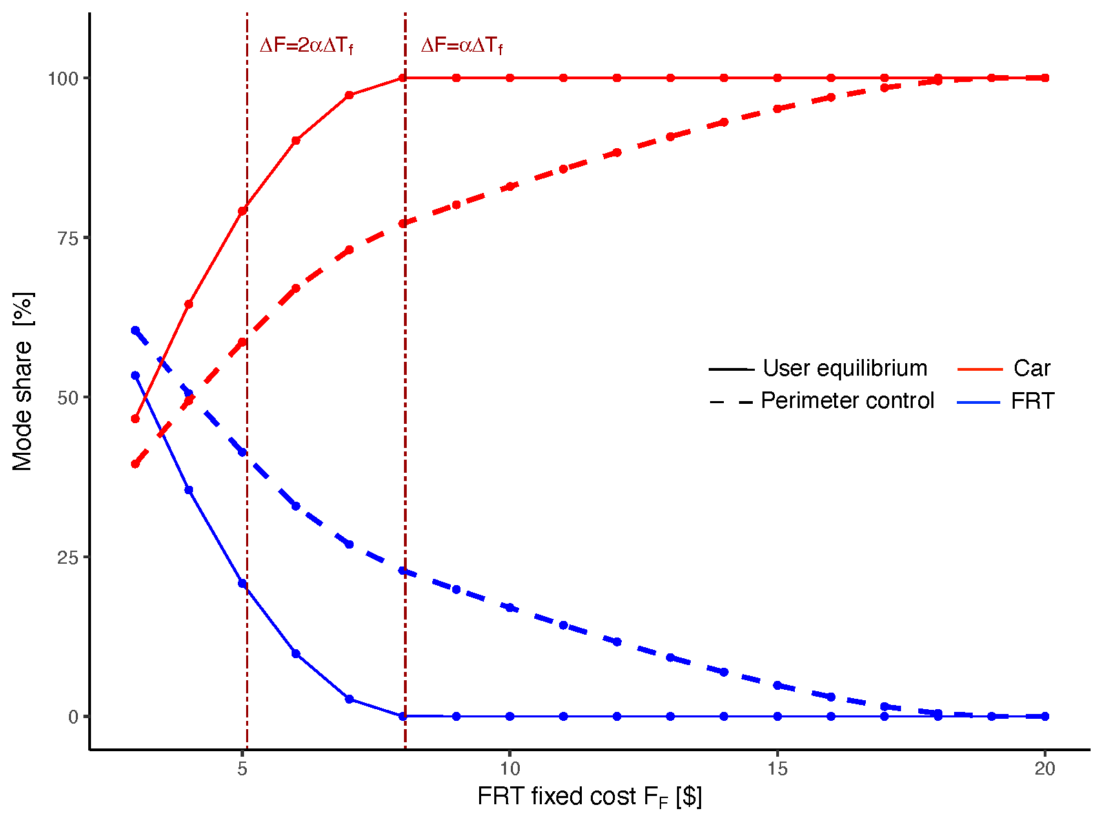
(a) Mode share

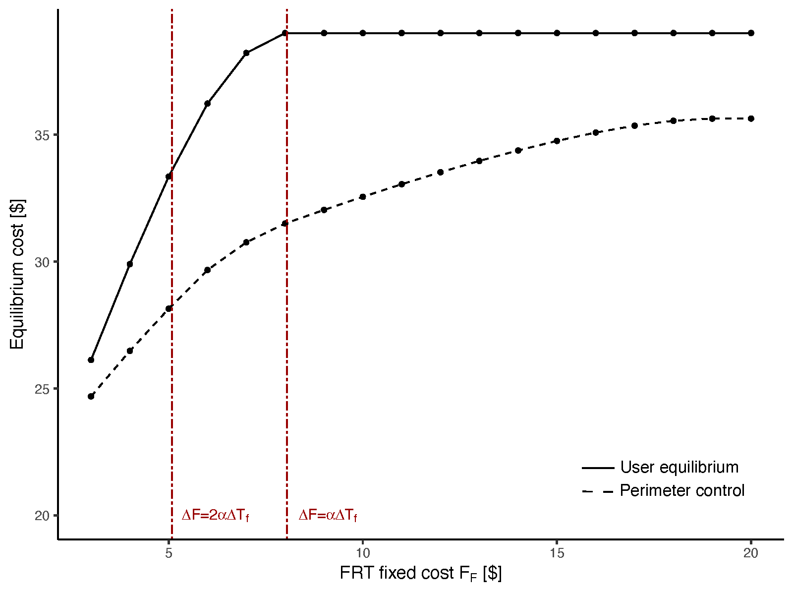
(b) Equilibrium cost

Figure 13: Sensitivity analysis to FRT fixed cost (the left and right vertical dotted lines represent the FRT fixed cost; $\displaystyle\Delta F=2\alpha\Delta T_{f}$ and $\displaystyle\Delta F=\alpha\Delta T_{f}$, respectively)

Table 2: Sensitivity analysis to FRT fixed cost

	User equilibrium		Perimeter control
$\displaystyle F_{F}$	$\displaystyle c^{*}$	FRT mode share [%]	$\displaystyle c_{p}^{*}$	FRT mode share [%]	$\displaystyle\frac{c_{p}^{*}}{c^{*}}$
3	26.1	53.3	24.7	60.5	0.95
5	33.4	20.9	28.1	41.4	0.84
8	39.0	0.0	31.5	22.8	0.81
10	39.0	0.0	32.6	17.0	0.83
15	39.0	0.0	34.8	4.9	0.89
20	39.0	0.0	35.6	0.0	0.91

6.2 Sensitivity analysis with respect to FRT fixed cost

Next, we conduct a sensitivity analysis with respect to the FRT fixed cost , as depicted in Fig. 13 and Table. 2. Note that we use $\displaystyle L_{F}=7$ [mile], $\displaystyle F_{c}=11$ [$], $\displaystyle N=200$ [pax] in this analysis. The left and right vertical dotted lines in Fig. 13 indicate the costs that yield $\displaystyle\Delta F=2\alpha\Delta T_{f}$; $\displaystyle F_{F}=5.09$ and $\displaystyle\Delta F=\alpha\Delta T_{f}$; $\displaystyle F_{F}=8.05$, respectively. The left side of the left line shows the case where FRT is used from the beginning to the end during rush hour, the middle part between the left and right lines shows the case where there is a time window wherein FRT is not used regardless of perimeter control, and the right side of the right line shows the case where FRT is never used at user equilibrium, whereas FRT is used, but there is a time window when FRT is not used at equilibrium with perimeter control. The equilibrium cost can be reduced by perimeter control in all cases from the user equilibrium cost. An increase in FRT fixed cost results in an increase in equilibrium cost under perimeter control because it increases the mode share of cars (Fig. 13 (a)) and lengthens the car rush hour. Transit priority is still beneficial, even in the case where FRT is never used at user equilibrium, In the case where the FRT fixed cost is higher than $\displaystyle 8.05$ [$], all commuters use their cars, and the FRT mode share is zero at user equilibrium (Fig. 13 (a) and Table. 2). Perimeter control with transit priority can increase the mode share of FRT. However, when the FRT fixed cost is too high (e.g., $\displaystyle F_{F}=20$ [$] as shown in Table. 2) , FRT is not used during perimeter control because $\displaystyle\theta_{p}>(2\alpha T_{f}^{F}-\Delta F)/(\alpha T_{f}^{c})$ is not satisfied, as verified in Proposition 5.3. Since the mode share is unchanged, the effect of perimeter control with transit priority is the same as that of perimeter control alone. Bimodality is not fully utilized in this case. Thus, additional incentives, such as fare reduction so that $\displaystyle\theta_{p}>(2\alpha T_{f}^{F}-\Delta F)/(\alpha T_{f}^{c})$ is satisfied, should be provided to promote FRT use during perimeter control.

To investigate the impact of perimeter control, we estimate the ratio of the equilibrium cost with perimeter control to the user equilibrium cost as shown in the last column of Table. 2. An increases in the FRT fixed cost increases the impact of perimeter control when $\displaystyle\Delta F>\alpha\Delta T_{f}$. This is because an increase in the FRT fixed cost increases the mode share of cars, leading to a longer duration of hypercongestion at user equilibrium. Thus, this causes longer perimeter control and increasing the impact of perimeter control. In contract, the higher the FRT fixed cost is, the lower will be the impact of perimeter control is when $\displaystyle\Delta F\leq\alpha\Delta T_{f}$. Since all commuters use their cars, the mode share and the duration of hypercongestion remain unchanged at user equilibrium regardless of the value of the FRT fixed cost. During perimeter control, an increase in the FRT fixed cost leads to a higher mode share of cars, and thus a higher equilibrium cost if $\displaystyle\theta_{p}>(2\alpha T_{f}^{F}-\Delta F)/(\alpha T_{f}^{c})$. Therefore, the impact of perimeter control decreases.

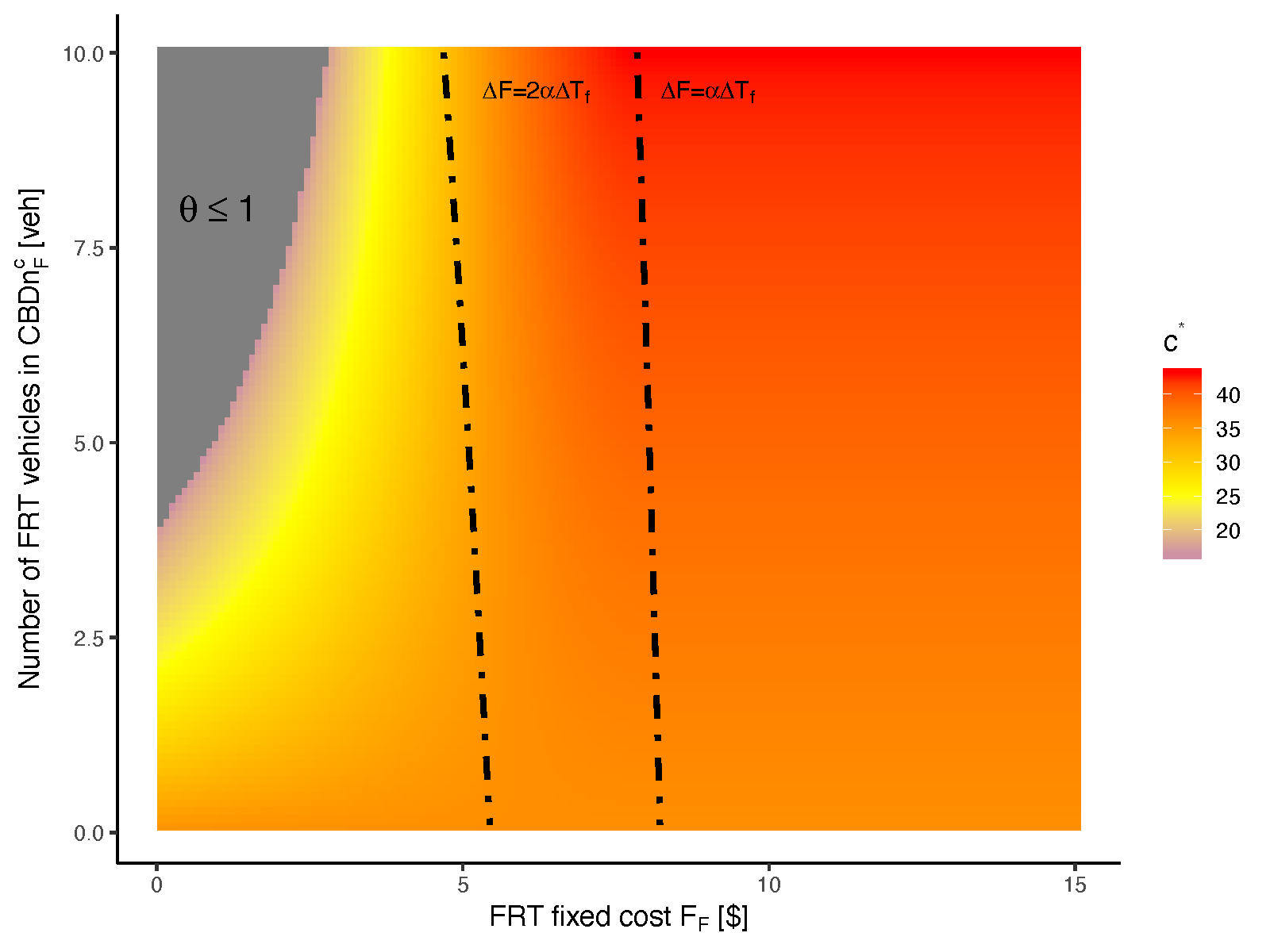
(a) User equilibrium

(b) Perimeter control

Figure 14: Sensitivity analysis of equilibrium cost

(a) User equilibrium

(b) Perimeter control

Figure 15: Sensitivity analysis of mode share

6.3 Sensitivity analysis with respect to number of FRT vehicles and FRT fixed cost

Further, we conduct a sensitivity analysis with respect to both of the number of FRT vehicles and FRT fixed cost to better understand the implications. Note that we use the same parameters as in Section 6.2. If many FRT vehicles are operated and FRT fixed cost is lowered (i.e., $\displaystyle\theta\leq 1$ in the gray coloured areas of Figs. 15 (a) and 15 (a)), all commuters will take FRT. Although an increase in the FRT fixed cost and a decrease in the number of FRT vehicles increase the mode share of cars, hypercongestion never occurs as long as $\displaystyle\theta\leq 2$ (the gray coloured areas of Figs. 15 (b) and 15 (b)). We also find that an increase in the number of FRT vehicles reduces the equilibrium cost when FRT fixed cost is lower at user equilibrium without perimeter control (see the left side of the dotted line which is the cost yielding $\displaystyle\Delta F=2\alpha\Delta T_{f}$ in Fig. 15 (a)). Because hypercongestion never occur or occur for a short period in most cases, an increase in the number of FRT vehicles simply alleviates the discomfort for FRT, thereby resulting in higher mode share of cars and shortening the rush hour. However, if the FRT fixed cost is high, hypercongestion occurs due to higher mode share of cars. An increase in the number of FRT vehicles leads to a severe capacity drop, resulting in a higher equilibrium cost. Moreover, the mode share of FRT does not increase significantly due to the network capacity effect in this case, as depicted in the middle part of the dotted lines in Fig. 15 (a)

When perimeter control is implemented, hypercongestion never occur. Therefore, even when the FRT fixed cost is the cost which yields $\displaystyle\Delta F<2\alpha\Delta T_{f}$ and $\displaystyle\Delta F>\alpha\Delta T_{f}$ (the middle part of the dotted lines in Fig. 15 (b)), the mode share of FRT can be increased due to an increase in the number of FRT vehicles, which results in a lower equilibrium cost as shown in Fig. 15 (b). However, as discussed in Section 6.1, even though an increase in the number of FRT vehicles increases the mode share of FRT, the equilibrium cost will increase only when the FRT fixed cost is higher (the right side of the dotted line which is the cost yielding $\displaystyle\Delta F=\alpha\Delta T_{f}$ in Fig. 15 (b)).

We showed that bimodality is an important component for efficient perimeter control, and can be enhanced by providing transit priority and incentives to lower the FRT fixed cost (if necessary). However, the operation of too many vehicles that reduces discomfort may produce an unintended result: operating many FRT vehicles may increase the equilibrium cost.

7 Conclusions

We investigated traveler behavior changes in response to perimeter control with transit priority in a bimodal transportation system (cars and flexible route transit (FRT)). To this end, we developed a bimodal bathtub model; it is a departure time and transportation mode choices model that incorporates the hypercongestion and FRT discomfort. First, some conditions of the equilibrium patterns were characterized: (I) If the difference of the car fixed cost from the FRT fixed cost is higher than the difference of the FRT travel time cost from the car travel time cost at free-flow, then both modes are used, and the FRT rush hour is longer than the car rush hour. (II) The number of FRT passengers decreases with time toward the desired arrival time. (III) There may be a time interval wherein FRT is not used around the rush hour peak. Then, we examined commuter behavior changes during perimeter control with transit priority. We found that if the fixed cost difference is larger than the travel time cost after perimeter control starts, then FRT is used during perimeter control; otherwise, FRT is not used during perimeter control. This implies that transit priority may not be sufficient to promote the use of FRT and that additional incentives may be required to promote FRT use during perimeter control. Finally, we conducted numerical analyses to investigate the equilibrium patterns of the model. We showed that operating many FRT vehicles to promote mode shift from cars during perimeter control may increase equilibrium cost

There are several directions for future works. Although we showed the theoretical results of the bimodal bathtub model, the empirical measurements that incorporate hypercongestion, discomfort of transit users and travel behavior need to be conducted. This analysis will elucidate our discussion further. Second, it would be interesting to extend the model to multiregion models. Since the regional route choice model will be considered, multiregion models that consider regional route, departure time, and transportation mode choices will no longer be tractable. Surrogate techniques (e.g., Ge et al., 2020; Dantsuji et al., 2022) can be used to address this issue. Third, although we assume free-flow conditions in the suburban zone for the tractability, recent research (e.g., Keyvan-Ekbatani et al., 2015) has shown the impact of the congestion propagation from the perimeter boundaries on the MFD dynamics in the suburban zone. Thus, a model extension in this direction would be an interesting. Finally, the urban structure was assumed to be fixed in this study. As urban structures change in response to traffic demand management (Takayama and Kuwahara, 2017; Fosgerau et al., 2018; Takayama, 2020), this would be an interesting direction.

Appendix A: Proof of Proposition 3

We prove that the equilibrium cost is uniquely determined in the case where there is a time window wherein FRT is not used. Let $\displaystyle F(\theta)$ be the RHS of Eq. (36) (i.e., $\displaystyle N=F(\theta)$). If the function of $\displaystyle F(\theta)$ is strictly monotonic with respect to $\displaystyle\theta$, then the equilibrium cost $\displaystyle c^{*}$ is uniquely determined. As $\displaystyle\theta$ is defined as the ratio of the sum of the travel time and schedule delay costs at equilibrium to the free-flow travel time, we have $\displaystyle\theta>1$. Thus, we prove the monotonicity of $\displaystyle F(\theta)$ for $\displaystyle\theta>1$. We derive the first derivative of $\displaystyle F(\theta)$ from Eq. (36) as

$$\displaystyle\frac{dF(\theta)}{d\theta}=\alpha n_{j}^{\prime}\left(\frac{1}{\beta}+\frac{1}{\gamma}\right)\left(\frac{1}{\theta}-\frac{1}{\theta^{2}}\right)$$ (72)

For $\displaystyle\theta>1$, $\displaystyle dF/d\theta$ is strictly monotonically increasing. Thus, the equilibrium cost is uniquely determined.

The first derivative of $\displaystyle F(\theta)$ from Eq. (39) for the case where FRT is used continuously during the FRT rush hour is

$$\displaystyle\frac{dF(\theta)}{d\theta}=\left(\frac{1}{\beta}+\frac{1}{\gamma}\right)\left(\alpha n_{j}^{\prime}\left(\frac{1}{\theta}-\frac{1}{\theta^{2}}\right)+n_{F}^{c}\frac{\alpha}{\lambda}\frac{T_{f}^{c}}{T_{f}^{F}}\left(\Delta F\frac{1}{\theta}+\alpha\Delta T_{f}\right)\right)$$ (73)

The condition for $\displaystyle dF/d\theta>0$ is

$$\displaystyle\alpha n_{j}^{\prime}\left(\frac{1}{\theta}-\frac{1}{\theta^{2}}\right)+n_{F}^{c}\frac{\alpha}{\lambda}\frac{T_{f}^{c}}{T_{f}^{F}}\left(\Delta F\frac{1}{\theta}+\alpha\Delta T_{f}\right)>0$$ (74)

Multiplication of $\displaystyle\theta^{2}$ and some tedious calculations yield

$$\displaystyle\alpha\Delta T_{f}n_{F}^{c}\frac{\alpha}{\lambda}\frac{T_{f}^{c}}{T_{f}^{F}}\theta^{2}+\left(\alpha n_{j}^{\prime}+\Delta Fn_{F}^{c}\frac{\alpha}{\lambda}\frac{T_{f}^{c}}{T_{f}^{F}}\right)\theta-\alpha n_{j}^{\prime}>0$$ (75)

This condition is satisfied for $\displaystyle\theta>1$. Thus, the equilibrium cost is uniquely determined.

Appendix B: Proof that perimeter control is never implemented if Assumption 1 holds and $\displaystyle\theta_{p}\leq(2\alpha T_{f}^{F}-\Delta F)/\alpha T_{f}^{c}$

As $\displaystyle\theta^{p}\equiv\frac{(c_{p}^{*}-F_{c})v_{f}^{\prime}}{\alpha L_{c}}$, $\displaystyle\theta_{p}\leq\frac{2\alpha T_{f}^{F}-\Delta F}{\alpha T_{f}^{c}}$ can be rewritten by

$$\displaystyle\frac{(c_{p}^{*}-F_{c})v_{f}^{\prime}}{\alpha L_{c}}\leq\frac{2\alpha T_{f}^{F}-\Delta F}{\alpha T_{f}^{c}}$$ (76)

Since $\displaystyle c_{p}^{*}=\alpha T_{f}^{c}+\beta(t^{*}-t_{s}^{c})+F_{c}$, Eq. (76) yields,

$$\displaystyle\beta(t^{*}-t_{s}^{c})-\alpha T_{f}^{F}\leq\alpha\Delta T_{f}-\Delta F$$ (77)

If Assumption 1 holds (i.e., $\displaystyle\Delta F>\alpha\Delta T_{f}$),

$$\displaystyle\beta(t^{*}-t_{s}^{c})-\alpha T_{f}^{F}<0$$ (78)

If perimeter control is implemented, the travel cost is equal to the equilibrium cost when car accumulation reaches the critical level. $\displaystyle c_{p}^{*}=2\alpha T_{f}^{c}+\beta(t^{*}-t_{s}^{p})+F_{c}=\alpha T_{f}^{c}+\beta(t^{*}-t_{s}^{c})+F_{c}$ yields,

$$\displaystyle\beta(t^{*}-t_{s}^{p})=\frac{1}{\beta}\left(\beta\left(t^{*}-t_{s}^{c}\right)-\alpha T_{f}^{c}\right)$$ (79)

As $\displaystyle\alpha T_{f}^{F}>\alpha T_{f}^{c}$ and $\displaystyle\beta(t^{*}-t_{s}^{c})-\alpha T_{f}^{F}<0$, the desired arrival time is earlier than the time when accumulation reaches the critical level (i.e., $\displaystyle(t^{*}-t_{s}^{p})<0$) if Assumption 1 holds. Thus, perimeter control is never implemented in this case.

Appendix C: Proof of Proposition 6

We prove that the equilibrium cost during perimeter control is uniquely determined in the case where FRT is used from the beginning to the end during the FRT rush hour. Let $\displaystyle F(\theta^{p})$ be the RHS of Eq. (65). Then, we have

$$\displaystyle\frac{dF(\theta^{p})}{d\theta^{p}}=\left(\frac{1}{\beta}+\frac{1}{\gamma}\right)\left(\frac{\alpha n_{j}^{\prime}}{4}+n_{F}^{c}\frac{\alpha}{\lambda}\frac{T_{f}^{c}}{2T_{f}^{F}}\alpha T_{f}^{c}(\theta^{p}-2)\right)$$ (80)

It yields

$$\displaystyle\frac{dF(\theta^{p})}{d\theta^{p}}=\begin{cases}\leq 0&\text{if }\theta^{p}\leq 2\left(1-\frac{\alpha n_{j}^{\prime}}{4}\frac{1}{n_{F}^{c}}\frac{\lambda}{\alpha}\frac{T_{f}^{F}}{T_{f}^{c}}\frac{1}{\alpha T_{f}^{c}}\right)\\ >0&\text{otherwise }\end{cases}$$ (81)

Combining this with the fact that $\displaystyle\theta^{p}>1$ and $\displaystyle F(1)=0$, since $\displaystyle\theta^{p}=1$ states that the equilibrium cost is equal to the free-flow travel time and fixed costs (equilibrium cost when $\displaystyle N=0$), produces a unique equilibrium cost.

Next, we prove that the equilibrium cost during perimeter control is uniquely determined in the case where FRT is used, but there will be a time window wherein FRT is not used during the FRT rush hour. Let $\displaystyle F(\theta^{p})$ be the RHS of Eq. (69). Then, the first derivative of $\displaystyle F(\theta^{p})$ is

$$\displaystyle\frac{dF(\theta^{p})}{d\theta^{p}}=\left(\frac{1}{\beta}+\frac{1}{\gamma}\right)\left(\frac{\alpha n_{j}^{\prime}}{4}+n_{F}^{c}\frac{\alpha}{\lambda}\frac{T_{f}^{c}}{2T_{f}^{F}}\alpha T_{f}^{c}\left(\theta^{p}-\frac{2\alpha T_{f}^{F}-\Delta F}{\alpha T_{f}^{c}}\right)\right)$$ (82)

It is positive since $\displaystyle\theta^{p}>\frac{2\alpha T_{f}^{F}-\Delta F}{\alpha T_{f}^{c}}$. Thus, $\displaystyle dF/d\theta^{p}>0$ yields a unique equilibrium cost.

Similarly, we can prove that the equilibrium cost is uniquely determined for Eqs. (70) and (71).

Appendix D: List of variables

Table 3: The list of notations in the paper

Notation	Description
$\displaystyle n_{F}$	Total number of FRT vehicles
$\displaystyle n_{F}^{s},n_{F}^{c}$	Number of FRT vehicles in the suburban and CBD zones, respectively
$\displaystyle v_{i}(t)$	Space-mean speed of transportation mode $\displaystyle i$ in the CBD zone
$\displaystyle v_{f}$	Free-flow car space-mean speed in the CBD zone
$\displaystyle n_{i}(t)$	Accumulation of mode $\displaystyle i$’s vehicles in the CBD zone
$\displaystyle\eta$	Passenger car unit
$\displaystyle n_{j}$	Jam accumulation
$\displaystyle n_{c}^{cr}$	Critical car accumulation ($\displaystyle=n_{j}^{{}^{\prime}}/2$)
$\displaystyle m$	Parameter that captures lower FRT’s speed than car’s speed in the CBD zone
$\displaystyle v_{f}^{\prime}$	$\displaystyle=v_{f}\left(1-\eta n_{F}^{c}/n_{j}\right)$
$\displaystyle n_{j}^{\prime}$	$\displaystyle=n_{j}\left(1-\eta n_{F}^{c}/n_{j}\right)$
$\displaystyle I_{c}(t)$	Car inflow rate to the CBD zone at time $\displaystyle t$
$\displaystyle I_{c}^{p}$	Inflow rate during perimeter control ($\displaystyle=n_{j}^{{}^{\prime}}v_{f}^{{}^{\prime}}/(4L_{c})$)
$\displaystyle G_{c}(t),G_{F}^{p}(t)$	Car and FRT passenger arrival rates at the destination at time $\displaystyle t$
$\displaystyle L_{i}$	Average trip length of mode $\displaystyle i$’s commuters in the CBD zone
$\displaystyle d_{F}(t)$	Departure rate of FRT passengers at time $\displaystyle t$
$\displaystyle C_{i}(t)$	Mode $\displaystyle i$’s travel cost incurred by a commuter who arrives at their destination at time $\displaystyle t$
$\displaystyle T_{i}(t)$	Travel time in the CBD zone of a commuter who arrives at time $\displaystyle t$ by transportation mode $\displaystyle i$
$\displaystyle T_{f}^{i}$	Mode $\displaystyle i$’s free-flow travel time in the CBD zone
$\displaystyle T_{i}^{s}$	Free-flow mode $\displaystyle i$’s travel time in the suburban zone
$\displaystyle p_{c},p_{F}$	Car operation cost and FRT fare, respectively
$\displaystyle F_{i}$	Fixed cost for transportation mode $\displaystyle i$
$\displaystyle\alpha,\beta,\gamma,\lambda$	Marginal costs for travel time, earliness, lateness, and discomfort, respectively
$\displaystyle g(t)$	Discomfort cost at time $\displaystyle t$
$\displaystyle\Delta F$	$\displaystyle=F_{c}-F_{F}$
$\displaystyle\Delta T_{f}$	$\displaystyle=T_{f}^{F}-T_{f}^{c}$
$\displaystyle c^{*},c_{p}^{*}$	Equilibrium cost without and with perimeter control
$\displaystyle\theta$	$\displaystyle\equiv(c^{*}-F_{c})v_{f}^{{}^{\prime}}/(\alpha L_{c})$
$\displaystyle\theta_{p}$	$\displaystyle\equiv(c^{*}_{p}-F_{c})v_{f}^{{}^{\prime}}/(\alpha L_{c})$
$\displaystyle t_{s}^{i},t_{e}^{i}$	Start and end times of mode $\displaystyle i$’s rush hour, respectively
$\displaystyle t_{ee}^{F},t_{sl}^{F}$	Start and end times of a time window wherein FRT is not used during the FRT rush hour, respectively
$\displaystyle t_{s}^{p},t_{e}^{p}$	Start and end times of perimeter control implemented
$\displaystyle N$	Total number of commuters
$\displaystyle N_{i}$	Total number of mode $\displaystyle i$’s commuters
$\displaystyle N_{i}^{p}$	Number of mode $\displaystyle i$’s commuters who arrives at their destination during perimeter control
$\displaystyle N_{F}^{oc}$	Number of commuters who take FRT outside the car rush hour
$\displaystyle N_{i}^{op}$	Number of mode $\displaystyle i$’s commuters outside the perimeter control period
$\displaystyle A_{b}(t)$	Car arrival rate at the perimeter boundary at time $\displaystyle t$
$\displaystyle T_{b}(t)$	Waiting time at the perimeter boundary of a commuter who arrives at their destination at time $\displaystyle t$
$\displaystyle q(t)$	Number of cars queued at the perimeter boundary when a commuter who arrives
	at their destination at time $\displaystyle t$ reaches the boundary

References

- Amirgholy and Gao (2017) Amirgholy, M., Gao, H. O., 2017. Modeling the dynamics of congestion in large urban networks using the macroscopic fundamental diagram: User equilibrium, system optimum, and pricing strategies. Transportation Research Part B: Methodological 104, 215–237.
- Ampountolas et al. (2017) Ampountolas, K., Zheng, N., Geroliminis, N., 2017. Macroscopic modelling and robust control of bi-modal multi-region urban road networks. Transportation Research Part B: Methodological 104, 616–637.
- Arnott (2013) Arnott, R., 2013. A bathtub model of downtown traffic congestion. Journal of Urban Economics 76, 110–121.
- Arnott and Buli (2018) Arnott, R., Buli, J., 2018. Solving for equilibrium in the basic bathtub model. Transportation Research Part B: Methodological 109, 150–175.
- Arnott et al. (1993) Arnott, R., de Palma, A., Lindsey, R., 1993. A structural model of peak-period congestion: A traffic bottleneck with elastic demand. The American Economic Review, 161–179.
- Bao et al. (2021) Bao, Y., Verhoef, E. T., Koster, P., 2021. Leaving the tub: The nature and dynamics of hypercongestion in a bathtub model with a restricted downstream exit. Transportation Research Part E: Logistics and Transportation Review 152, 102389.
- Bartholdi III and Eisenstein (2012) Bartholdi III, J. J., Eisenstein, D. D., 2012. A self-coördinating bus route to resist bus bunching. Transportation Research Part B: Methodological 46 (4), 481–491.
- Basso et al. (2019) Basso, L. J., Feres, F., Silva, H. E., 2019. The efficiency of bus rapid transit (brt) systems: A dynamic congestion approach. Transportation Research Part B: Methodological 127, 47–71.
- Chen et al. (2022a) Chen, S., Fu, H., Wu, N., Wang, Y., Qiao, Y., 2022a. Passenger-oriented traffic management integrating perimeter control and regional bus service frequency setting using 3d-pmfd. Transportation Research Part C: Emerging Technologies 135, 103529.
- Chen et al. (2022b) Chen, Z., Wu, W.-X., Huang, H.-J., Shang, H.-Y., 2022b. Modeling traffic dynamics in periphery-downtown urban networks combining vickrey’s theory with macroscopic fundamental diagram: user equilibrium, system optimum, and cordon pricing. Transportation Research Part B: Methodological 155, 278–303.
- Chiabaut (2015) Chiabaut, N., 2015. Evaluation of a multimodal urban arterial: The passenger macroscopic fundamental diagram. Transportation Research Part B: Methodological 81, 410–420.
- Daganzo (2007) Daganzo, C. F., 2007. Urban gridlock: Macroscopic modeling and mitigation approaches. Transportation Research Part B: Methodological 41 (1), 49–62.
- Daganzo and Pilachowski (2011) Daganzo, C. F., Pilachowski, J., 2011. Reducing bunching with bus-to-bus cooperation. Transportation Research Part B: Methodological 45 (1), 267–277.
- Dakic and Menendez (2018) Dakic, I., Menendez, M., 2018. On the use of lagrangian observations from public transport and probe vehicles to estimate car space-mean speeds in bi-modal urban networks. Transportation Research Part C: Emerging Technologies 91, 317–334.
- Dantsuji et al. (2021) Dantsuji, T., Fukuda, D., Zheng, N., 2021. Simulation-based joint optimization framework for congestion mitigation in multimodal urban network: a macroscopic approach. Transportation 48 (2), 673–697.
- Dantsuji et al. (2020) Dantsuji, T., Hirabayashi, S., Ge, Q., Fukuda, D., 2020. Cross comparison of spatial partitioning methods for an urban transportation network. International Journal of Intelligent Transportation Systems Research 18, 412–421.
- Dantsuji et al. (2022) Dantsuji, T., Hoang, N. H., Zheng, N., Vu, H. L., 2022. A novel metamodel-based framework for large-scale dynamic origin–destination demand calibration. Transportation Research Part C: Emerging Technologies 136, 103545.
- de Palma et al. (2017) de Palma, A., Lindsey, R., Monchambert, G., 2017. The economics of crowding in rail transit. Journal of Urban Economics 101, 106–122.
- Ding et al. (2017) Ding, H., Guo, F., Zheng, X., Zhang, W., 2017. Traffic guidance–perimeter control coupled method for the congestion in a macro network. Transportation Research Part C: Emerging Technologies 81, 300–316.
- Fosgerau (2015) Fosgerau, M., 2015. Congestion in the bathtub. Economics of Transportation 4 (4), 241–255.
- Fosgerau et al. (2018) Fosgerau, M., Kim, J., Ranjan, A., 2018. Vickrey meets alonso: Commute scheduling and congestion in a monocentric city. Journal of Urban Economics 105, 40–53.
- Fosgerau and Small (2013) Fosgerau, M., Small, K. A., 2013. Hypercongestion in downtown metropolis. Journal of Urban Economics 76, 122–134.
- Fu et al. (2020) Fu, H., Wang, Y., Tang, X., Zheng, N., Geroliminis, N., 2020. Empirical analysis of large-scale multimodal traffic with multi-sensor data. Transportation Research Part C: Emerging Technologies 118, 102725.
- Ge et al. (2020) Ge, Q., Fukuda, D., Han, K., Song, W., 2020. Reservoir-based surrogate modeling of dynamic user equilibrium. Transportation Research Part C: Emerging Technologies 113, 350–369.
- Genser and Kouvelas (2022) Genser, A., Kouvelas, A., 2022. Dynamic optimal congestion pricing in multi-region urban networks by application of a multi-layer-neural network. Transportation Research Part C: Emerging Technologies 134, 103485.
- Geroliminis (2015) Geroliminis, N., 2015. Cruising-for-parking in congested cities with an mfd representation. Economics of Transportation 4 (3), 156–165.
- Geroliminis and Daganzo (2008) Geroliminis, N., Daganzo, C. F., 2008. Existence of urban-scale macroscopic fundamental diagrams: Some experimental findings. Transportation Research Part B: Methodological 42 (9), 759–770.
- Geroliminis et al. (2012) Geroliminis, N., Haddad, J., Ramezani, M., 2012. Optimal perimeter control for two urban regions with macroscopic fundamental diagrams: A model predictive approach. IEEE Transactions on Intelligent Transportation Systems 14 (1), 348–359.
- Geroliminis and Levinson (2009) Geroliminis, N., Levinson, D. M., 2009. Cordon pricing consistent with the physics of overcrowding. In: Transportation and Traffic Theory 2009: Golden Jubilee. Springer, pp. 219–240.
- Geroliminis et al. (2014) Geroliminis, N., Zheng, N., Ampountolas, K., 2014. A three-dimensional macroscopic fundamental diagram for mixed bi-modal urban networks. Transportation Research Part C: Emerging Technologies 42, 168–181.
- Giuliano (1992) Giuliano, G., 1992. An assessment of the political acceptability of congestion pricing. Transportation 19 (4), 335–358.
- Godfrey (1969) Godfrey, J., 1969. The mechanism of a road network. Traffic Engineering & Control 8 (8).
- Gonzales (2015) Gonzales, E. J., 2015. Coordinated pricing for cars and transit in cities with hypercongestion. Economics of Transportation 4 (1-2), 64–81.
- Gonzales and Daganzo (2012) Gonzales, E. J., Daganzo, C. F., 2012. Morning commute with competing modes and distributed demand: user equilibrium, system optimum, and pricing. Transportation Research Part B: Methodological 46 (10), 1519–1534.
- Gonzales and Daganzo (2013) Gonzales, E. J., Daganzo, C. F., 2013. The evening commute with cars and transit: Duality results and user equilibrium for the combined morning and evening peaks. Transportation Research Part B: Methodological 57 (C), 286–299.
- Gu et al. (2018) Gu, Z., Liu, Z., Cheng, Q., Saberi, M., 2018. Congestion pricing practices and public acceptance: A review of evidence. Case Studies on Transport Policy 6 (1), 94–101.
- Guo and Ban (2020) Guo, Q., Ban, X. J., 2020. Macroscopic fundamental diagram based perimeter control considering dynamic user equilibrium. Transportation Research Part B: Methodological 136, 87–109.
- Haddad (2017) Haddad, J., 2017. Optimal perimeter control synthesis for two urban regions with aggregate boundary queue dynamics. Transportation Research Part B: Methodological 96, 1–25.
- Haddad and Geroliminis (2012) Haddad, J., Geroliminis, N., 2012. On the stability of traffic perimeter control in two-region urban cities. Transportation Research Part B: Methodological 46 (9), 1159–1176.
- Haddad and Shraiber (2014) Haddad, J., Shraiber, A., 2014. Robust perimeter control design for an urban region. Transportation Research Part B: Methodological 68, 315–332.
- Haitao et al. (2019) Haitao, H., Yang, K., Liang, H., Menendez, M., Guler, S. I., 2019. Providing public transport priority in the perimeter of urban networks: A bimodal strategy. Transportation Research Part C: Emerging Technologies 107, 171–192.
- Hamm et al. (2022) Hamm, L. S., Loder, A., Tilg, G., Menendez, M., Bogenberger, K., 2022. Network inefficiency: Empirical findings for six european cities. Transportation Research Record, 03611981221082588.
- Ji and Geroliminis (2012) Ji, Y., Geroliminis, N., 2012. On the spatial partitioning of urban transportation networks. Transportation Research Part B: Methodological 46 (10), 1639–1656.
- Jin (2020) Jin, W.-L., 2020. Generalized bathtub model of network trip flows. Transportation Research Part B: Methodological 136, 138–157.
- Keyvan-Ekbatani et al. (2015) Keyvan-Ekbatani, M., Yildirimoglu, M., Geroliminis, N., Papageorgiou, M., 2015. Multiple concentric gating traffic control in large-scale urban networks. IEEE Transactions on Intelligent Transportation Systems 16 (4), 2141–2154.
- Lamotte and Geroliminis (2018) Lamotte, R., Geroliminis, N., 2018. The morning commute in urban areas with heterogeneous trip lengths. Transportation Research Part B: Methodological 117, 794–810.
- Li et al. (2021) Li, Y., Yildirimoglu, M., Ramezani, M., 2021. Robust perimeter control with cordon queues and heterogeneous transfer flows. Transportation Research Part C: Emerging Technologies 126, 103043.
- Liu and Geroliminis (2016) Liu, W., Geroliminis, N., 2016. Modeling the morning commute for urban networks with cruising-for-parking: An mfd approach. Transportation Research Part B: Methodological 93, 470–494.
- Loder et al. (2017) Loder, A., Ambühl, L., Menendez, M., Axhausen, K. W., 2017. Empirics of multi-modal traffic networks–using the 3d macroscopic fundamental diagram. Transportation Research Part C: Emerging Technologies 82, 88–101.
- Loder et al. (2019) Loder, A., Ambühl, L., Menendez, M., Axhausen, K. W., 2019. Understanding traffic capacity of urban networks. Scientific reports 9 (1), 1–10.
- Loder et al. (2022) Loder, A., Bliemer, M. C., Axhausen, K. W., 2022. Optimal pricing and investment in a multi-modal city—introducing a macroscopic network design problem based on the mfd. Transportation Research Part A: Policy and Practice 156, 113–132.
- Mahmassani et al. (1987) Mahmassani, H., Williams, J. C., Herman, R., 1987. Performance of urban traffic networks. In: Proceedings of the 10th International Symposium on Transportation and Traffic Theory. Vol. 14. Elsevier Amsterdam, The Netherlands, pp. 1–20.
- Ni and Cassidy (2020) Ni, W., Cassidy, M., 2020. City-wide traffic control: modeling impacts of cordon queues. Transportation research part C: emerging technologies 113, 164–175.
- Paipuri et al. (2021) Paipuri, M., Barmpounakis, E., Geroliminis, N., Leclercq, L., 2021. Empirical observations of multi-modal network-level models: Insights from the pneuma experiment. Transportation Research Part C: Emerging Technologies 131, 103300.
- Ramezani et al. (2015) Ramezani, M., Haddad, J., Geroliminis, N., 2015. Dynamics of heterogeneity in urban networks: aggregated traffic modeling and hierarchical control. Transportation Research Part B: Methodological 74, 1–19.
- Simoni et al. (2015) Simoni, M. D., Pel, A. J., Waraich, R. A., Hoogendoorn, S. P., 2015. Marginal cost congestion pricing based on the network fundamental diagram. Transportation Research Part C: Emerging Technologies 56, 221–238.
- Sipetas and Gonzales (2021) Sipetas, C., Gonzales, E. J., 2021. Continuous approximation model for hybrid flexible transit systems with low demand density. Transportation Research Record 2675 (8), 198–214.
- Sirmatel and Geroliminis (2017) Sirmatel, I. I., Geroliminis, N., 2017. Economic model predictive control of large-scale urban road networks via perimeter control and regional route guidance. IEEE Transactions on Intelligent Transportation Systems 19 (4), 1112–1121.
- Small and Chu (2003) Small, K. A., Chu, X., 2003. Hypercongestion. Journal of Transport Economics and Policy (JTEP) 37 (3), 319–352.
- Takayama (2020) Takayama, Y., 2020. Who gains and who loses from congestion pricing in a monocentric city with a bottleneck? Economics of Transportation 24, 100189.
- Takayama and Kuwahara (2017) Takayama, Y., Kuwahara, M., 2017. Bottleneck congestion and residential location of heterogeneous commuters. Journal of Urban Economics 100, 65–79.
- Tirachini et al. (2014) Tirachini, A., Hensher, D. A., Rose, J. M., 2014. Multimodal pricing and optimal design of urban public transport: The interplay between traffic congestion and bus crowding. Transportation research part b: methodological 61, 33–54.
- Vansteenwegen et al. (2022) Vansteenwegen, P., Melis, L., Aktaş, D., Montenegro, B. D. G., Vieira, F. S., Sörensen, K., 2022. A survey on demand-responsive public bus systems. Transportation Research Part C: Emerging Technologies 137, 103573.
- Velaga et al. (2012) Velaga, N. R., Beecroft, M., Nelson, J. D., Corsar, D., Edwards, P., 2012. Transport poverty meets the digital divide: accessibility and connectivity in rural communities. Journal of Transport Geography 21, 102–112.
- Vickrey (2020) Vickrey, W., 2020. Congestion in midtown manhattan in relation to marginal cost pricing. Economics of Transportation 21, 100152.
- Wardrop (1952) Wardrop, J. G., 1952. Road paper. some theoretical aspects of road traffic research. Proceedings of the institution of civil engineers 1 (3), 325–362.
- Wu and Huang (2014) Wu, W.-X., Huang, H.-J., 2014. Equilibrium and modal split in a competitive highway/transit system under different road-use pricing strategies. Journal of Transport Economics and Policy (JTEP) 48 (1), 153–169.
- Xu et al. (2018) Xu, S.-X., Liu, R., Liu, T.-L., Huang, H.-J., 2018. Pareto-improving policies for an idealized two-zone city served by two congestible modes. Transportation Research Part B: Methodological 117, 876–891.
- Yang and Huang (2005) Yang, H., Huang, H.-J., 2005. Mathematical and economic theory of road pricing.
- Yildirimoglu et al. (2021) Yildirimoglu, M., Ramezani, M., Amirgholy, M., 2021. Staggered work schedules for congestion mitigation: A morning commute problem. Transportation Research Part C: Emerging Technologies 132, 103391.
- Yildirimoglu et al. (2015) Yildirimoglu, M., Ramezani, M., Geroliminis, N., 2015. Equilibrium analysis and route guidance in large-scale networks with mfd dynamics. Transportation Research Part C 59, 404–420.
- Yildirimoglu et al. (2018) Yildirimoglu, M., Sirmatel, I. I., Geroliminis, N., 2018. Hierarchical control of heterogeneous large-scale urban road networks via path assignment and regional route guidance. Transportation Research Part B: Methodological 118, 106–123.
- Zheng et al. (2017) Zheng, N., Dantsuji, T., Wang, P., Geroliminis, N., 2017. Macroscopic approach for optimizing road space allocation of bus lanes in multimodal urban networks through simulation analysis. Transportation Research Record 2651 (1), 42–51.
- Zheng and Geroliminis (2013) Zheng, N., Geroliminis, N., 2013. On the distribution of urban road space for multimodal congested networks. Transportation Research Part B: Methodological 57 (C), 326–341.
- Zheng and Geroliminis (2020) Zheng, N., Geroliminis, N., 2020. Area-based equitable pricing strategies for multimodal urban networks with heterogeneous users. Transportation Research Part A: Policy and Practice 136, 357–374.
- Zheng et al. (2012) Zheng, N., Waraich, R. A., Axhausen, K. W., Geroliminis, N., 2012. A dynamic cordon pricing scheme combining the macroscopic fundamental diagram and an agent-based traffic model. Transportation Research Part A: Policy and Practice 46 (8), 1291–1303.
- Zheng et al. (2018) Zheng, Y., Li, W., Qiu, F., 2018. A slack arrival strategy to promote flex-route transit services. Transportation Research Part C: Emerging Technologies 92, 442–455.