An example of use of Variational Methods in Quantum Machine Learning

Abstract

This paper introduces a deep learning system based on a quantum neural network for the binary classification of points of a specific geometric pattern (Two-Moons Classification problem) on a plane.

We believe that the use of hybrid deep learning systems (classical + quantum) can reasonably bring benefits, not only in terms of computational acceleration but in understanding the underlying phenomena and mechanisms; that will lead to the creation of new forms of machine learning, as well as to a strong development in the world of quantum computation.

The chosen dataset is based on a 2D binary classification generator, which helps test the effectiveness of specific algorithms; it is a set of 2D points forming two interspersed semicircles. It displays two disjointed data sets in a two-dimensional representation space: the features are, therefore, the individual points’ two coordinates, $x_{1}$ and $x_{2}$.

The intention was to produce a quantum deep neural network with the minimum number of trainable parameters capable of correctly recognising and classifying points.

1 Introduction

The stages of knowledge in the history of humankind have always alternated between amazement at the immensity of the phenomenon before us and the joyful conquest for the objectives set. The development and introduction into the science of a powerful mathematical arsenal have slowly enabled many obstacles to be overcome, confirming Galileo’s intuition that mathematics is the straightforward language that enables us to dialogue with nature. At the beginning of the 20th century, our optimism in positivist determinism was strongly shaken by new phenomena that led to the birth of quantum mechanics. Nevertheless, the observation of the generation of deterministic chaos from models with a seemingly simple apparatus of differential equations and the evident need to describe basic molecular structures by simulating them with automatic calculation tools that require ever-increasing computational capabilities are suggesting that the time has come for a profound reflection on our tools of scientific investigation. Feynman stated that describing the reality that surrounds us, which has an intrinsically quantum nature, through a type of computation based on quantum mechanics would be the key to exponentially lowering the computational complexity of the system in question and correctly managing the predictive capacity for the model. We might also add that the introduction of quantum computing machines would also solve the problems related to the imminent reaching of the construction limit of current computers (Amdahl’s law), to the possibility of a drastic reduction in the energy required by today’s computing machines thanks to computational reversibility, and to the development of nanotechnology.

The possibility of such opportunities has resulted in a growing international interest in such devices, with considerable funding in the relevant research areas. Quantum Computing machines can therefore respond to questions that would be unimaginable for actual old-style apparatuses [1], as they would need the whole Universe’s existence time to complete the same task. That is allowed by some quantum peculiarities that show up at the littlest of scales, like Superposition, Entanglement and Interference [2]. Although the theoretical study of quantum algorithms suggests the real possibility of solving computational problems that are currently intractable [3], the current technology has not reached maturity, such as to obtain truly appreciable advantages. We are still in the so-called era of Noisy Intermediate-Scale Quantum (NISQ) [4]. NISQ-devices are noisy and have limited quantum resources; this presents various obstacles when implementing a gate-based quantum algorithm. In order to determine if an implementation of a gate-based algorithm would run effectively on a particular NISQ-device, numerous aspects of circuit implementation, such as depth, width, and noise, should be considered [5, 6].

Variational Methods [7, 8] are widely used in physics, and most of all in quantum mechanics [9]. Their direct successors, Variational Quantum Algorithms (VQAs), have appeared to be the most effective technique for gaining a quantum advantage on NISQ devices. VQAs are undoubtedly the quantum equivalent of very effective machine-learning techniques like neural networks. Furthermore, VQAs use the classical optimisation toolbox since they employ parametrised quantum circuits to run on the quantum computer and then outsource parameter optimisation to a classical optimiser. In contrast to quantum algorithms built for the fault-tolerant time period, this technique provides the extra benefits of keeping the quantum circuit depth small and minimising noise [10].

The aim is to find the exact, or a well-approximated, parameter values’ set that minimises a given cost (loss) function, which depends on the parameters themselves and, naturally, on the input values, x; these are the non-trainable part of the schema. An output measurement apparatus and a parameter modulation circuit serve as regulators (Fig.1).

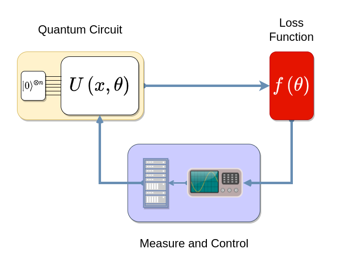
Figure 1: Scheme

In our specific case, we are dealing with a n-qubits quantum ansatz, whose transformation is represented by the $n\times n$ unitary matrix U that depends on the vector of parameters $\theta$, with dimensions $m\;\epsilon\;\mathbb{N}$ (eq. (1)); the loss function we refer to is the expectation value measured on every single qubit channel (eq. (3)); the observable is the operator $O_{i}$, where $Z_{i}$ is the Z-Pauli Operator, acting on i-th qubit (eq. (2)); the quantum state on which to operate the measurements will be the state resulting from the ansatz ($\psi$ in eq. (1)).

$$\Big{|}\psi\left(\textbf{$\overline{\theta}$}\;\right)\Big{\rangle}=U\left(\textbf{$\overline{\theta}$}\;\right)\cdot|0\rangle^{\otimes n}$$ (1)

$$O_{i}=Z_{i}\>,\hskip 10.00002pti\;\epsilon\>\left\{1..n\right\}\subset\mathbb{N}$$ (2)

$$\Big{\langle}E_{i}\left(\textbf{$\overline{\theta}$}\;\right)\Big{\rangle}=\left\langle\psi^{\dagger}\left(\textbf{$\overline{\theta}$}\;\right)\,\Big{|}\;O_{i}\,\Big{|}\;\psi\left(\textbf{$\overline{\theta}$}\;\right)\right\rangle$$ (3)

It is well-known that Quantum Computers can take care of specific issues quicker than traditional ones. As it may, stacking information into a quantum computer is not paltry. It should be encoded in quantum bits (qubits) to stack the information. There are multiple ways qubits can address the data, and, in this manner, various information encodings are conceivable [11]. Several methods can embed data: Basis Encoding [12, 13], Amplitude Encoding [14, 15, 16], and Angle Encoding [17, 18] are the most common to implant information into a firstly prepared quantum state.

Our work aims to explore aspects of the usability of quantum computation in machine learning. Specifically, we sought to compare the performance of a basic FFNN with dense layers and an analogous network composed of quantum components in learning a simple classification problem.

2 Related works

The possibility of using machine learning techniques in quantum computing has been gaining ground since 2010 [19, 20, 21]. The incorporation of quantum algorithms into machine learning programmes is known as quantum machine learning [22, 23, 24, 25]. The expression is most commonly used to refer to machine learning methods for evaluating classical data run on a quantum computer. While machine learning techniques are used to calculate vast quantities of data, quantum machine learning employs qubits and quantum operations or specialised quantum systems to speed up computing [26] and data storage [27]. Quantum machine learning also refers to an area of study investigating the theoretical and functional analogies between specific physical systems and learning systems, namely neural networks [28].

Unfortunately, the current technological development does not yet allow the full potential of quantum computers to be expressed, which will only reach maturity in the next few decades. At present, however, it is possible to use quantum computers in feedback circuits that mitigate the effect of various noise components [29, 30]. VQAs, which utilise a conventional optimiser to train a parameterised quantum circuit, have been considered an effective technique for addressing these restrictions.

The core part of the computational stage consists of a sequence of gates applied to specified wires in variational circuits. Like the design of a neural network that merely describes the basic structure, the variational approach can optimise the types of gates and their free parameters. In time, the quantum computing community has suggested several variational circuit types that can distinguish three main base structures, depending on the shape of the ansatz: layered gate ansatz [31], alternating operator ansatz [32, 33], and tensor network ansatz [34].

The first type of architecture inspired us in implementing our network, trying to keep the network simple, with a minimum number of quantum gates and trainable parameters.

3 The architecture of the system

Our network has a general structure of this type:

• A first classical dense layer, to accept features as input

• A quantum circuit formed by a succession of rotational and entanglement gates

• A final classical dense layer for classification

Our quantum structure differs from some other proposals, which encodes input features to transform them into quantum states [35, 36]; our initial state, the ”prepared state”, is simply $|0\rangle^{\otimes n}$. Our architecture is based on the typical ”Prepared State fixed; Ansatz parametrised” model. Several variants exist in the literature, especially the most known Instantaneous Quantum Polynomial (IQP) circuits [37]. The initial dense network, which we called input-layer, acts as an interface between the input data and the quantum layer; its output directly drives the internal rotations of the quantum state, attributing new values to the rotation angles at each epoch (Fig. 2).

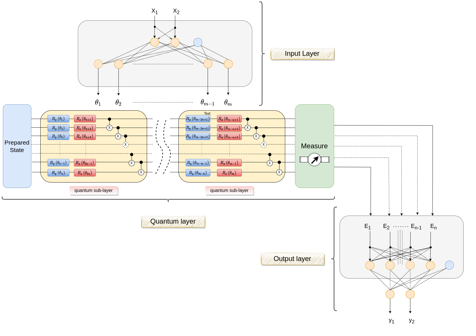
Figure 2: Architecture of the quantum neural network

Almost all the simulations were conducted using quantum sub-layers consisting of a first stack of rotation gates around the Y-axis of the Bloch’s sphere, a second stack of rotation gate around the Z-axis and a chain of cX gates (CNOT) to maximise the entanglement effect. Rotation operators help primarily to ensure the expressibility of a parameterized quantum circuit. That is essentially the total coverage of Hilbert space by the hypothesis space of the ansatz itself [38]. In addition, the chain of CNOT operators is tasked with maximising the entanglement effect of individual qubits, as the entanglement phenomenon plays a crucial role in quantum computation. This feature is called Entangling Capability [39].

An authentic advantage is that the network’s response remains independent of the number of qubits. The only real quantum noise remains due to the construction and constitution of the ansatz and the device, or simulator, used for experimentation.

3.1 Data extraction and processing

The database chosen for the classification problem is called two-moons, which generates two interleaving semicircles of 2D-points, and is characteristic for the study of clustering and classification algorithms.

The dataset was generated thanks to the dedicated function from the Python Scikit-Learn library.

The input domain is $\left[-2.0,3.0\right]\times\left[-2.0,2.5\right]\subset\mathbb{R}^{2}$. One thousand samples were randomly generated, equally distributed over the two classes. The classes were initially chosen with a Gaussian Error Coefficient of 0.05: this coefficient quantifies the capacity of separation of the two categories: the higher its value, the greater the degree of overlap of the two classes (Fig. 3).

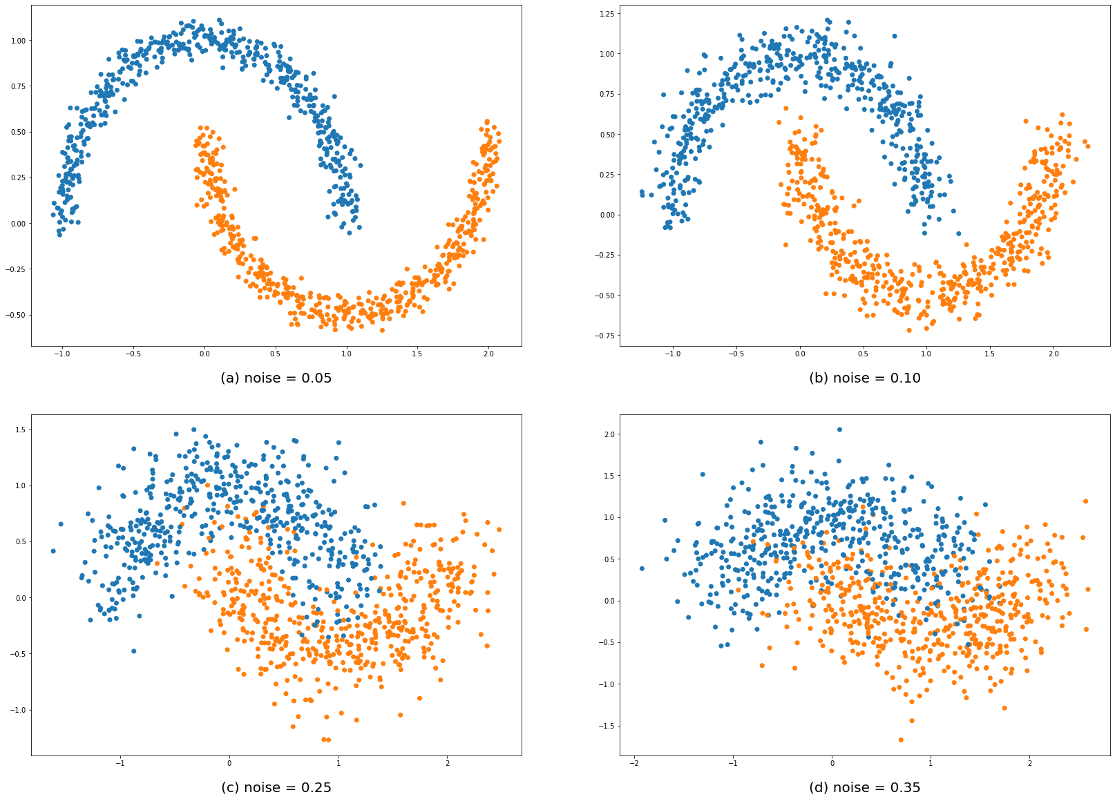
Figure 3: Distribution of pattern points on the plane in relation to Gaussian Noise

The number of samples in the dataset was divided in such a way as to ensure the following quotas: 70% for the training set, 20% for the validation set and the remaining 10% for the test set.

3.2 Model construction and validation

Two twin models have been realised in parallel, using for one of them the Python library for quantum simulation Cirq with TensorFlowQuantum, by Google, and for the other an open-source Python library, PennyLane, by Xanadu, which can be perfectly interfaced with the most famous Deep Learning frameworks, such as Keras, and of course TensorFlow, and PyTorch.

All tests and simulations were performed using the specialised open-source library for Deep Learning, Keras.

The TFQ (TensorFlowQuantum) model is composed as follows (Fig. 4a):

• A layer for data input, called input_layer.

• A Dense layer, which adapts the input to the number of parameters, in our specific case 16, called FFNN.

• A layer for the ansatz input in the form of a tensor, called qc_layer.

• A control layer (called TOTAL), which receives the two inputs, modulates the values of the parameters and returns, for each wire in the circuit, the expected value.

• A final Dense layer (called output_layer), with a number of outputs equal to the number of classes in the dataset, which returns the probability of belonging to them (softmax activation).

The PQML (PennyLane Quantum Machine Learning) model is composed as follows (Fig. 4b):

• A layer for data input, called DATA.

• A Dense layer, which adapts the input to the number of parameters, in our specific case 16, called layer1.

• A custom layer, called quantum_layer, designed as a subclass of the Layer class from the Keras library, which receives in input the values of the parameters of the ansatz and returns, for each wire of the circuit, the expected value.

• A final Dense layer (called output_layer), with a number of outputs equal to the number of classes in the dataset, which returns the probability of belonging to them (softmax activation).

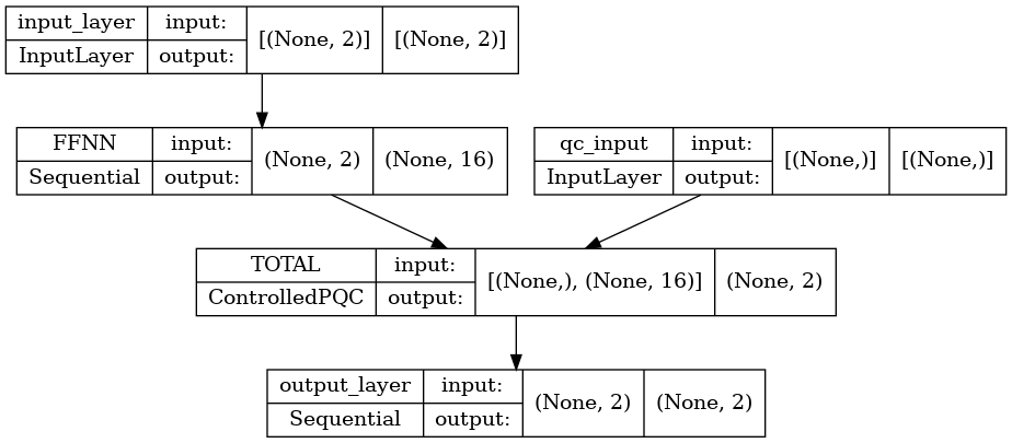
(a) TQF Model

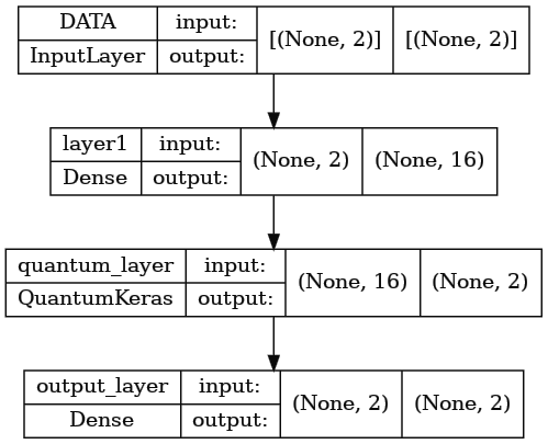
(b) PQML Model

Figure 4: Quantum Neural Network Models utilised

The number of ansatz parameters is given by the product of the number of qubits, the number of rotation operators acting on each line of the circuit within each sublayer, and the number of sublayers. For our tests and simulations, we have opted to use an ansatz consisting of 4 sublayers to avoid creating an excessive computational load on the quantum layer. By initially constraining the number of qubits to 2 and not introducing any form of noise, we can say that both models proved to be extremely light in terms of the number of trainable parameters: 54 against the 354 of a similar FFNN Fully-Connected, with three layers. The disadvantage is that the simulation run times are about one order of magnitude longer than the latter. In fact, to simulate an ansatz is necessary to operate many matrix products against only one matrix product for a standard dense layer.

The entire model was compiled using a classical optimiser, SGD (Stochastic Gradient Descent), with Mean Absolute Error as the Loss Function and Accuracy as the metric.

3.3 Analysis of results

The results obtained are excellent. Figure 5 shows the metrics (LOSS: loss function on training set, ACCURACY: accuracy on training set, VAL_LOSS: loss function on validation set, VAL_ACCURACY: accuracy on validation set,) for the TFQ model, trained for 20 epochs, with different values of Gaussian Noise on the dataset generation (legend).

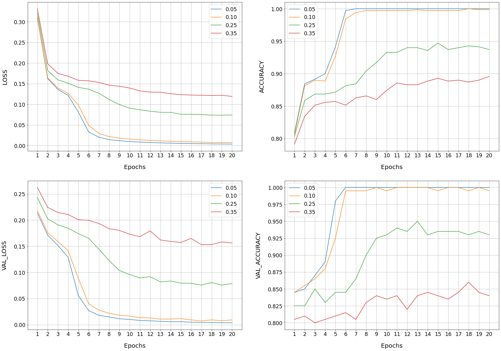
Figure 5: Metrics for TFQ model

The model achieves 100% accuracy for low-noise datasets and more than 80% accuracy for high-noise datasets.

	[HTML]656565 Samples: 20 / 200			[HTML]656565 Samples: 100 / 1,000			[HTML]656565 Samples: 500 / 5,000
[HTML]C0C0C0                [HTML]A5E4F7					[HTML]C0C0C0n qubits			[HTML]C0C0C0n qubits			[HTML]C0C0C0n qubits
[HTML]C0C0C0                [HTML]A5E4F7NOISE					[HTML]C0C0C02	[HTML]C0C0C03	[HTML]C0C0C04	[HTML]C0C0C02	[HTML]C0C0C03	[HTML]C0C0C04	[HTML]C0C0C02	[HTML]C0C0C03	[HTML]C0C0C04
[HTML]A5E4F70.05	100.0 %	95.0 %	95.0 %	100.0 %	100.0 %	100.0 %	100.0 %	100.0 %	100.0 %
[HTML]A5E4F70.10	100.0 %	95.0 %	95.0 %	100.0 %	100.0 %	100.0 %	100.0 %	100.0 %	100.0 %
[HTML]A5E4F70.25	95.0 %	80.0 %	90.0 %	93.0%	94.0 %	94.0 %	93.8 %	93.8 %	90.0 %
[HTML]A5E4F70.35	80.0 %	75.0 %	85.0 %	88.0%	86.0 %	89.0 %	88.4 %	88.6 %	88.4 %

Table 1: Percentage of correct evaluations on the test set for TFQ model.

Table 3.3 shows the percentages of correct evaluations on the test set as a function of the Gaussian Noise on the dataset, the number of qubits used, datasets with different cardinalities (the header of the table shows the number of samples of the test set on the number of total samples). It is referred to TFQ model.

Figure 6 shows the usual metrics for the PQML model, trained for 20 epochs, with different values of Gaussian Noise on the dataset generation (legend).

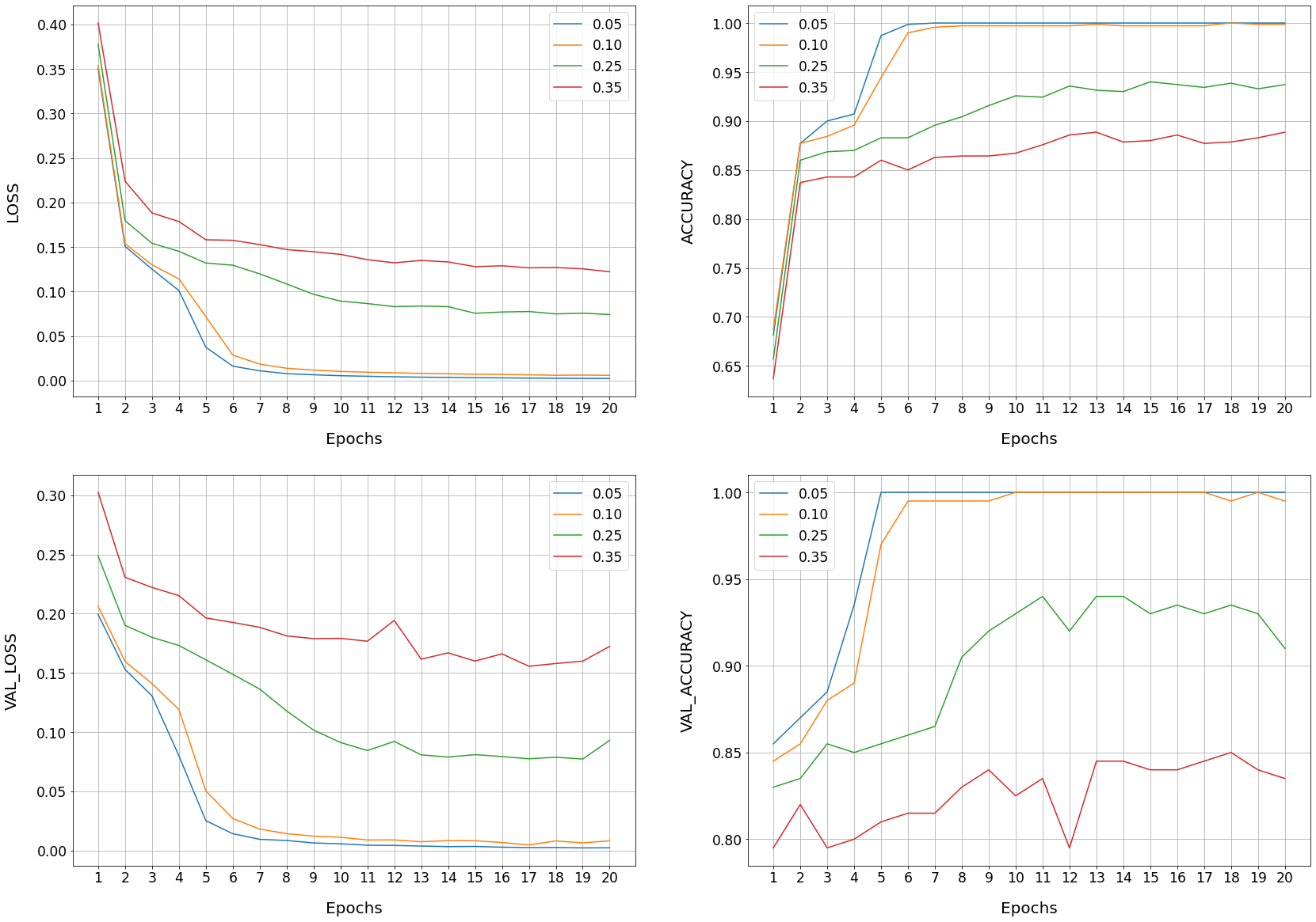
Figure 6: Metrics for PQML model

The model achieves 100% accuracy for low-noise datasets and beyond 80% accuracy for high-noise datasets.

	[HTML]656565 Samples: 20 / 200			[HTML]656565 Samples: 100 / 1,000			[HTML]656565 Samples: 500 / 5,000
[HTML]C0C0C0                [HTML]A5E4F7					[HTML]C0C0C0n qubits			[HTML]C0C0C0n qubits			[HTML]C0C0C0n qubits
[HTML]C0C0C0                [HTML]A5E4F7NOISE					[HTML]C0C0C02	[HTML]C0C0C03	[HTML]C0C0C04	[HTML]C0C0C02	[HTML]C0C0C03	[HTML]C0C0C04	[HTML]C0C0C02	[HTML]C0C0C03	[HTML]C0C0C04
[HTML]A5E4F70.05	100.0 %	100.0 %	95.0 %	100.0 %	100.0 %	100.0 %	100.0 %	100.0 %	100.0 %
[HTML]A5E4F70.10	95.0 %	100.0 %	95.0 %	100.0 %	100.0 %	100.0 %	100.0 %	100.0 %	100.0 %
[HTML]A5E4F70.25	95.0 %	100.0 %	80.0 %	94.0%	93.0 %	94.0 %	94.8 %	94.0 %	93.8 %
[HTML]A5E4F70.35	75.0 %	90.0 %	75.0 %	87.0%	88.0 %	86.0 %	88.2 %	88.4 %	87.2 %

Table 2: Percentage of correct evaluations on the test set for PQML model.

Table 3.3 shows the percentages of correct evaluations on the test set as a function of the Gaussian Noise on the dataset, the number of qubits used, datasets with different cardinalities (the header of the table shows the number of samples of the test set on the number of total samples). It is referred to PQML model.

Figure 7 shows the usual metrics for a simple FFNN Fully-Connected, three dense layers, with the same inputs and output as quantum networks, trained for 20 epochs and with 354 trainable weights. Without the use of regularisers or drop-out layers, an early overfitting of the model can be observed.

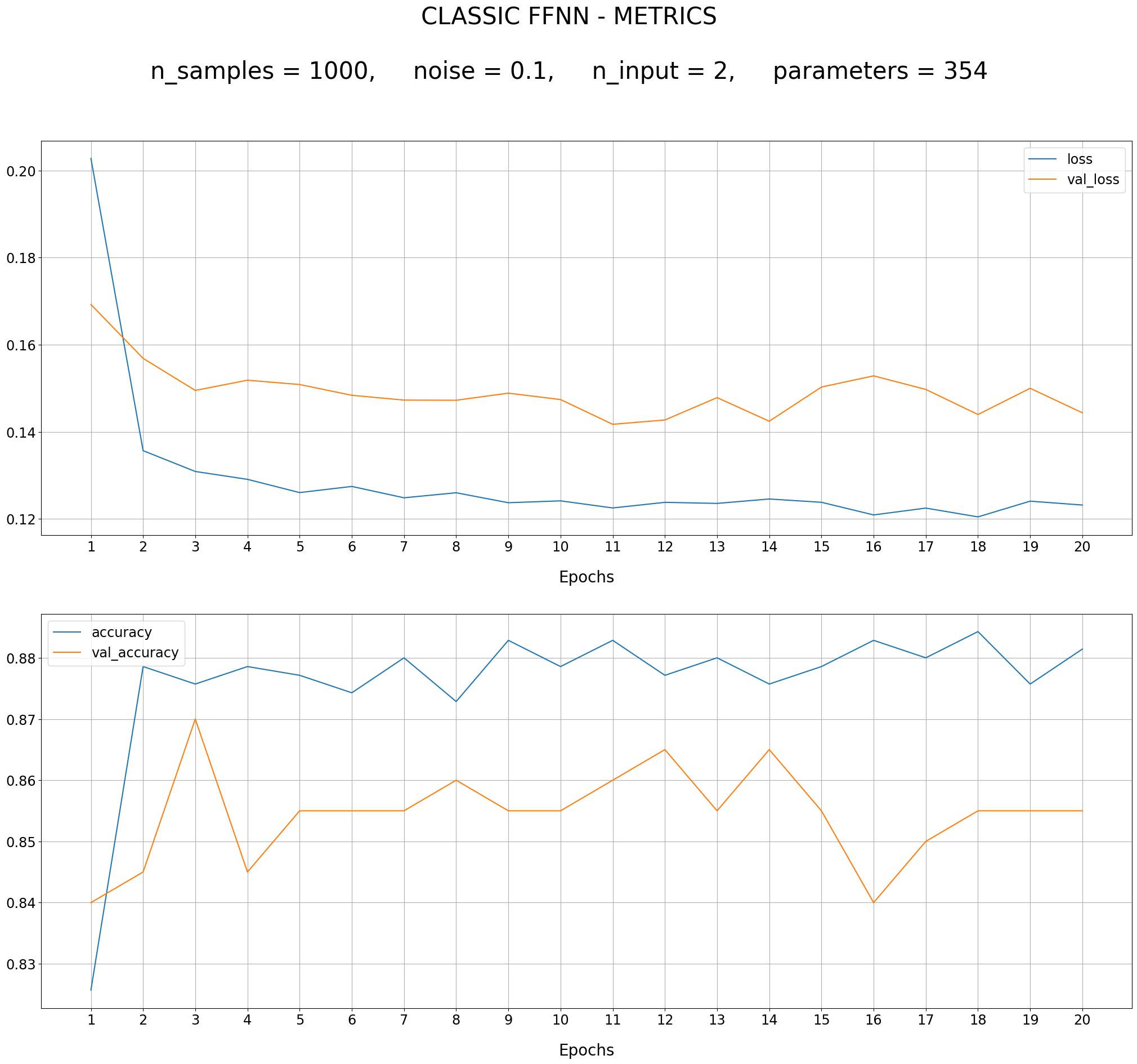
Figure 7: Metrics for an analogue FFNN

4 Conclusions and future works

The two models exhibit remarkably similar tendencies, demonstrating their quality and validity.

Interestingly, unlike an analogous FFNN, a quantum network, since it contains only unitary transformations, can reduce the overfitting phenomenon without the necessity of introducing any particular regularizers or drop-out layers (at least for certain values of ansatz depth).

In our future works, we intend to continue our investigations into quantum neural networks, working on various fronts: new datasets, different ansatz topologies, optimisers and loss functions. Since we focused our attention on some implementation aspects in this paper, ending up working on quantum simulators, we intend to conduct further tests on real machines (e.g. IBM Quantum Experience or Google’s Sycamore). We would like to understand better the real effects of quantum noise on circuits.

References

- [1] David Deutsch and Richard Jozsa “Rapid solution of problems by quantum computation” In Proceedings of the Royal Society of London. Series A: Mathematical and Physical Sciences 439.1907 The Royal Society London, 1992, pp. 553–558
- [2] Lov K Grover “Quantum mechanics helps in searching for a needle in a haystack” In Physical review letters 79.2 APS, 1997, pp. 325
- [3] Peter W Shor “Polynomial-time algorithms for prime factorization and discrete logarithms on a quantum computer” In SIAM review 41.2 SIAM, 1999, pp. 303–332
- [4] John Preskill “Quantum computing in the NISQ era and beyond” In Quantum 2 Verein zur Förderung des Open Access Publizierens in den Quantenwissenschaften, 2018, pp. 79
- [5] Frank Leymann and Johanna Barzen “The bitter truth about gate-based quantum algorithms in the NISQ era” In Quantum Science and Technology 5.4 IOP Publishing, 2020, pp. 044007
- [6] Marie Salm, Johanna Barzen, Frank Leymann and Benjamin Weder “About a criterion of successfully executing a circuit in the NISQ era: what really means” In Proceedings of the 1st ACM SIGSOFT International Workshop on Architectures and Paradigms for Engineering Quantum Software, 2020, pp. 10–13
- [7] Eberhard Zeidler “Nonlinear functional analysis and its applications: III: variational methods and optimization” Springer Science & Business Media, 2013
- [8] Donald R Smith “Variational methods in optimization” Courier Corporation, 1998
- [9] Riccardo Borghi “The variational method in quantum mechanics: an elementary introduction” In European Journal of Physics 39.3 IOP Publishing, 2018, pp. 035410
- [10] Marco Cerezo et al. “Variational quantum algorithms” In Nature Reviews Physics 3.9 Nature Publishing Group, 2021, pp. 625–644
- [11] Manuela Weigold, Johanna Barzen, Frank Leymann and Marie Salm “Data encoding patterns for quantum computing” In Proceedings of the 27th Conference on Pattern Languages of Programs, 2020, pp. 1–11
- [12] Vlatko Vedral, Adriano Barenco and Artur Ekert “Quantum networks for elementary arithmetic operations” In Physical Review A 54.1 APS, 1996, pp. 147
- [13] John A Cortese and Timothy M Braje “Loading classical data into a quantum computer” In arXiv preprint arXiv:1803.01958, 2018
- [14] Ryan LaRose and Brian Coyle “Robust data encodings for quantum classifiers” In Physical Review A 102.3 APS, 2020, pp. 032420
- [15] Aram W Harrow, Avinatan Hassidim and Seth Lloyd “Quantum algorithm for linear systems of equations” In Physical review letters 103.15 APS, 2009, pp. 150502
- [16] Maria Schuld, Mark Fingerhuth and Francesco Petruccione “Implementing a distance-based classifier with a quantum interference circuit” In EPL (Europhysics Letters) 119.6 IOP Publishing, 2017, pp. 60002
- [17] Manuela Weigold, Johanna Barzen, Frank Leymann and Marie Salm “Expanding data encoding patterns for quantum algorithms” In 2021 IEEE 18th International Conference on Software Architecture Companion (ICSA-C), 2021, pp. 95–101 IEEE
- [18] Edward Grant et al. “Hierarchical quantum classifiers” In npj Quantum Information 4.1 Nature Publishing Group, 2018, pp. 1–8
- [19] Seth Lloyd, Masoud Mohseni and Patrick Rebentrost “Quantum algorithms for supervised and unsupervised machine learning” In arXiv preprint arXiv:1307.0411, 2013
- [20] Nathan Wiebe, Ashish Kapoor and Krysta Svore “Quantum algorithms for nearest-neighbor methods for supervised and unsupervised learning” In arXiv preprint arXiv:1401.2142, 2014
- [21] Seth Lloyd, Masoud Mohseni and Patrick Rebentrost “Quantum principal component analysis” In Nature Physics 10.9 Nature Publishing Group, 2014, pp. 631–633
- [22] Damiano Perri et al. “Binary classification of proteins by a machine learning approach” In International Conference on Computational Science and Its Applications, 2020, pp. 549–558 Springer
- [23] Priscilla Benedetti et al. “Skin cancer classification using inception network and transfer learning” In International Conference on Computational Science and Its Applications, 2020, pp. 536–545 Springer
- [24] Damiano Perri et al. “A new method for binary classification of proteins with Machine Learning” In International Conference on Computational Science and Its Applications, 2021, pp. 388–397 Springer
- [25] Damiano Perri, Marco Simonetti and Osvaldo Gervasi “Synthetic Data Generation to Speed-Up the Object Recognition Pipeline” In Electronics 11.1 MDPI, 2021, pp. 2
- [26] Seokwon Yoo, Jeongho Bang, Changhyoup Lee and Jinhyoung Lee “A quantum speedup in machine learning: finding an N-bit Boolean function for a classification” In New Journal of Physics 16.10 IOP Publishing, 2014, pp. 103014
- [27] Yingkai Ouyang “Quantum storage in quantum ferromagnets” In Physical Review B 103.14 APS, 2021, pp. 144417
- [28] Kwok Ho Wan et al. “Quantum generalisation of feedforward neural networks” In npj Quantum information 3.1 Nature Publishing Group, 2017, pp. 1–8
- [29] Kishor Bharti et al. “Noisy intermediate-scale quantum algorithms” In Reviews of Modern Physics 94.1 APS, 2022, pp. 015004
- [30] Suguru Endo, Zhenyu Cai, Simon C Benjamin and Xiao Yuan “Hybrid quantum-classical algorithms and quantum error mitigation” In Journal of the Physical Society of Japan 90.3 The Physical Society of Japan, 2021, pp. 032001
- [31] Maria Schuld and Nathan Killoran “Quantum machine learning in feature hilbert spaces” In Physical review letters 122.4 APS, 2019, pp. 040504
- [32] Edward Farhi, Jeffrey Goldstone and Sam Gutmann “A quantum approximate optimization algorithm” In arXiv preprint arXiv:1411.4028, 2014
- [33] Guillaume Verdon, Michael Broughton and Jacob Biamonte “A quantum algorithm to train neural networks using low-depth circuits” In arXiv preprint arXiv:1712.05304, 2017
- [34] William Huggins et al. “Towards quantum machine learning with tensor networks” In Quantum Science and technology 4.2 IOP Publishing, 2019, pp. 024001
- [35] Jonathan Romero, Jonathan P Olson and Alan Aspuru-Guzik “Quantum autoencoders for efficient compression of quantum data” In Quantum Science and Technology 2.4 IOP Publishing, 2017, pp. 045001
- [36] Maria Schuld, Alex Bocharov, Krysta M Svore and Nathan Wiebe “Circuit-centric quantum classifiers” In Physical Review A 101.3 APS, 2020, pp. 032308
- [37] Dan Shepherd and Michael J Bremner “Instantaneous quantum computation” In arXiv preprint arXiv:0809.0847, 2008
- [38] Sukin Sim, Peter D Johnson and Alán Aspuru-Guzik “Expressibility and entangling capability of parameterized quantum circuits for hybrid quantum-classical algorithms” In Advanced Quantum Technologies 2.12 Wiley Online Library, 2019, pp. 1900070
- [39] Thomas Hubregtsen, Josef Pichlmeier, Patrick Stecher and Koen Bertels “Evaluation of parameterized quantum circuits: on the relation between classification accuracy, expressibility, and entangling capability” In Quantum Machine Intelligence 3.1 Springer, 2021, pp. 1–19