AutoShape: An Autoencoder-Shapelet Approach for Time Series Clustering

Abstract

Time series shapelets are discriminative subsequences that have been recently found effective for time series clustering (tsc). The shapelets are convenient for interpreting the clusters. Thus, the main challenge for tsc is to discover high-quality variable-length shapelets to discriminate different clusters. In this paper, we propose a novel autoencoder-shapelet approach (AutoShape), which is the first study to take the advantage of both autoencoder and shapelet for determining shapelets in an unsupervised manner. An autoencoder is specially designed to learn high-quality shapelets. More specifically, for guiding the latent representation learning, we employ the latest self-supervised loss to learn the unified embeddings for variable-length shapelet candidates (time series subsequences) of different variables, and propose the diversity loss to select the discriminating embeddings in the unified space. We introduce the reconstruction loss to recover shapelets in the original time series space for clustering. Finally, we adopt Davies–Bouldin index (DBI) to inform AutoShape of the clustering performance during learning. We present extensive experiments on AutoShape. To evaluate the clustering performance on univariate time series (uts), we compare AutoShape with $15$ representative methods using UCR archive datasets. To study the performance of multivariate time series (mts), we evaluate AutoShape on $30$ UEA archive datasets with $5$ competitive methods. The results validate that AutoShape is the best among all the methods compared. We interpret clusters with shapelets, and can obtain interesting intuitions about clusters in two uts case studies and one mts case study, respectively.

I Introduction

Time series clustering (tsc) has numerous applications in both academia and industry [1, 13, 16], and thus many research approaches [2, 12, 25] for solving tsc have been proposed. The classical approaches to solving the tsc problem can be categorized as whole series-based, feature-based, and model-based [22, 38, 49]. These approaches use the raw time series themselves, feature extraction, and model parameter transformation, and then apply K-means, DBSCAN, or other clustering algorithms. A recent trend in tsc is to find some local patterns or features from raw time series data. Among these approaches, shapelet-based methods (e.g., [39, 47, 48]) have repeatedly demonstrated their superior performance on tsc. Figure 1 shows an example of the shapelet $S_{1}$ discovered by AutoShape from one UCR uts dataset, i.e., ItalyPowerDemand [7].

In the seminal work on shapelets [43], they are discriminative time series subsequences, providing interpretable results, although shapelets are initially proposed for the classification problem on time series. The interpretability from shapelets has also been gauged by the cognitive metrics with respect to human [23]. The unsupervised-shapelet (a.k.a. u-shapelet) is first learned from unlabeled time series data for time series clustering in [47]. Scalable u-shapelet method [39] has been proposed for concerning the efficiency issue of shapelet discovery in tsc. To further improve clustering quality, Zhang et al. introduced an unsupervised model for learning shapelets, called USSL [48]. STCN [28] is proposed to optimize the feature extraction and self-supervised clustering simultaneously.

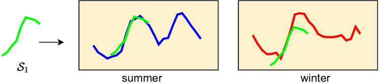
Figure 1: The shapelet $S_{1}$ for ItalyPowerDemand [7], which was derived from daily electrical power consumption time series from Italy in 1997. Two classes are in the dataset, summer (blue) from April to September, winter (red) from October to March.

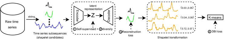
Figure 2: The overview of AutoShape for time series clustering (tsc). After time series subsequences (shapelet candidates) generation using sliding windows, \raisebox{-.9pt} {1}⃝ $\mathcal{L}_{Self-supervised}$ learns latent representations ${\bf Z}$ for time series subsequences to capture their characteristics. \raisebox{-.9pt} {2}⃝ $\mathcal{L}_{Diversity}$ selects the shapelets with both universality and heterogeneity. \raisebox{-.9pt} {3}⃝ $\mathcal{L}_{Reconstruction}$ makes the reconstruction of the latent representations to preserve the shapes of the shapelets. Then, the selected shapelets (black and green ones) are exploited to transform the original time series (orange color) into the transformed representations (using vectors to represent the transformed representations). The clustering algorithm (K-means) is applied to the transformed representations. \raisebox{-.9pt} {4}⃝ $\mathcal{L}_{DBI}$ is computed from the clustering results and used to adjust the shapelets, to improve the final clustering performance.

Recently, autoencoder-based methods (e.g., DEC [40], IDEC [14]) have been applied to the clustering problem and produce effective results. They optimize a clustering objective for learning a mapping from the raw data space to a lower-dimensional space. However, they are developed for the text and image clustering, not for time series. Some of autoencoder-based methods (e.g., DTC [30] and DTCR [29]) are then proposed for time series. They utilize an autoencoder network to learn general representations of whole time series instances under several different objectives. The trained encoder network is naturally employed to embed the raw time series into the new representations, which are used to replace the raw data for final clustering (e.g., K-means). Nonetheless, they focus on whole time series instances, ignore the importance of local features (time series subsequences) and miss the reasoning of clustering, namely interpretability [5].

Different from the above-mentioned autoencoder-based works, we learn a unified representation for variable-length time series subsequences (namely, shapelet candidates) of different variables. After all the shapelet candidates are embedded into the same latent space, it becomes simple to measure the similarity among the candidates and to further determine shapelets for clustering. Importantly, because of the autoencoder approach, shapelets are no longer restricted to real time series subsequences, which enlarges the scope of shapelet discovery from the raw data [43].

In this paper, we propose a novel autoencoder-based shapelet approach for tsc problem, called AutoShape. To the best of our knowledge, this is the first study to take the advantage of both shapelet-based methods and autoencoder-based methods for tsc. An overview of AutoShape is presented in Figure 2.

Four objectives are specially designed for learning the final shapelets for clustering. First, the self-supervised loss learns general unified embeddings of time series subsequences (shapelet candidates). Specifically, we employ a cluster-wise triplet loss [20], which has been shown effective for representing time series. Second, we propose a diversity loss to learn top-$k$ candidates after clustering all the embeddings. The learned candidates, closest to the centroid of a cluster, are of high quality that have two characteristics: they yield large clusters, and the clusters are distant from each other. Third, we decode the selected embeddings through the reconstruction loss to obtain decoded shapelets. Such shapelets maintain the shapes of the original time series subsequences for human interpretation. Then, the original time series are transformed with respect to the decoded shapelets. The new transformed representations are passed to construct a clustering model (e.g., K-means). Fourth, after achieving the clustering result, the Davies–Bouldin index (DBI) [8] is calculated to adjust the shapelets.

An autoencoder network is applied to jointly learn the time series subsequences representations to select high-quality shapelets for the transformation. Our shapelets for transformation are decoded by the autoencoder, not necessarily restricted to the raw time series. At the same time, the reconstruction loss of AutoShape  maintains the shapes of raw time series subsequences in the final shapelets, rather than learning some subsequences very different from the original time series.

We conduct comprehensive experiments on both univariate time series (UCR archive) [7] and multivariate time series (UEA archive) [3]. The results show that in terms of normalized mutual information (NMI) and rand index (RI) [48], AutoShape is the best of all $15$ and $6$ representative methods compared on univariate and multivariate time series (uts and mts), respectively. We note that AutoShape performs the best in $15$ out of $36$ uts datasets and $24$ out of $30$ mts datasets. Furthermore, an ablation study verifies the effectiveness of self-supervised loss, diversity loss and DBI objective. We present three cases from UCR archive (human motion recognition, power demand, and image) and one case from UEA archive (EEG of human activity recognition) to illustrate the intuitions of the learned shapelets.

The main contributions of this paper are summarized as follows:

• We propose an autoencoder-based shapelet approach, AutoShape, to jointly learn the time series subsequences representations for discovering discriminative shapelets for tsc in an unsupervised manner.

• Four objectives, namely, the self-supervised loss for latent representations, diversity loss for both universality and heterogeneity, reconstruction loss to preserve the shapes, and DBI objective to improve the final clustering performance, are specially designed for learning the final shapelets for clustering.

• Extensive experiments on UCR (uts) datasets and UEA (mts) datasets for tsc verify that our AutoShape is significantly more competitive in terms of accuracy when compared to the state-of-the-art methods.

• The interpretability of the learned shapelets, which may not be the real subsequences from raw time series data, is illustrated in four case studies on uts and mts datasets.

Organization. The rest of this paper is organized as follows. Section II reviews the related work. The details of our proposed method are given in Section III. Section IV reports the experimental results on both uts and mts. Section V concludes the paper and presents the future work.

II Related work

Interested readers may refer to some excellent review papers on time series clustering [1, 25]. In this section, we focus on the shapelet-based and autoencoder-based methods.

II-A Shapelet-based methods

The shapelet-based method was introduced with an emphasis on its interpretability in [43], and then studies on logical shapelets [31], shapelet transformation [27], learning shapelets [11], Matrix Profile [45], and efficient learning shapelets [18, 21] are mainly proposed for time series classification. The unsupervised-shapelet method (a.k.a u-shapelet) was proposed for time series clustering in [47]. Scalable u-shapelet method, a hash-based algorithm to discover u-shapelets efficiently, was introduced by Ulanova et al. [39]. The optimized techniques of SAX [26] have been exploited in scalable u-shapelet. k-Shape [32] relies on a scalable iterative refinement procedure to generate homogeneous and well-separated clusters. A normalized cross-correlation measure to calculate the distance of two time series is employed in k-Shape. Zhang et al. [48] proposed an unsupervised salient subsequence learning (USSL) model for tsc, which incorporates shapelet learning, shapelet regularization, spectral analysis and pseudo labeling. USSL is similar to the learning time series shapelets method for classification (i.e., LTS [11]). Self-supervised time series clustering network (STCN) [28] optimizes the feature extraction with one-step time series prediction conducted by RNN to capture the temporal dynamics and maintain the local structures of time series.

Unsupervised-shapelets are discovered without label information, and thus shapelets can been used for not only time series classification but also time series clustering. Li et al. [20] proposed the ShapeNet framework to discover shapelets for multivariate time series classification. In comparison, this paper is the first work to investigate how to discover shapelets to do the clustering on both univariate and multivariate time series.

II-B Autoencoder-based methods

Deep embedding clustering (DEC) [40] is a general method that simultaneously learns feature representations and cluster assignments for many data-driven application domains using deep neural networks. After learning the low-dimensional feature space, a clustering objective is optimized iteratively. Guo et al. [14] discovered that the defined clustering loss may corrupt the feature space and thus cause meaningless representations. Their proposed algorithm, the improved deep embedding clustering (IDEC), can preserve the structure of the data generating distribution with an under-complete autoencoder. Deep temporal clustering (DTC) [30] naturally integrates an autoencoder network for dimensionality reduction and a novel temporal clustering layer for new time series representation clustering into a single end-to-end learning framework without using labels. DTCR [29] proposes a seq2seq autoencoder representation learning model, integrating reconstruction task (for autoencoder), K-means task (for hidden representation), and classification task (to enhance the ability of encoder). After learning the autoencoder, a classical method (e.g.,  K-means) is applied to the hidden representation. As we shall see, this paper specially designs loss functions for an autoencoder to determine shapelets for time series clustering.

III Autoencoder for shapelets (AutoShape)

In this section, we propose an autoencoder-based shapelet approach, called AutoShape. As the name suggests, AutoShape adopts the autoencoder network for shapelet discovery. It learns the unified embeddings of shapelet candidates and meanwhile preserves original time series subsequences’ shapes to make it possible to understand the intuitions of the clusters. More specifically, we exploit an autoencoder network to learn the general unified embeddings of time series subsequences (shapelet candidates) using four objectives, namely \raisebox{-.9pt} {1}⃝ self-supervised loss, \raisebox{-.9pt} {2}⃝ diversity loss, \raisebox{-.9pt} {3}⃝ reconstruction loss and \raisebox{-.9pt} {4}⃝ Davies–Bouldin index (DBI) objective. We jointly learn the shapelets with all the four objectives without labels. We summarize the notations used and their meanings in Table I.

TABLE I: Summary of frequently used notations

Notation	Meaning
$T$	a univariate time series (uts) instance
	$T=(t_{1},t_{2},\cdots,t_{i},\cdots,t_{N})$,
	where $t_{i}$ is the $i$-th value in $T$
	and $N$ is the length of $T$
$D$	a uts dataset $(T_{1},T_{2},\cdots,T_{M})$,
	where $M$ is the number of time series in $D$
$T_{a,b}$	a subsequence $T_{a,b}$ of $T$, $(t_{a},\cdots,t_{b})$,
	where $1\leq a\leq b\leq N$,
	$a$ and $b$, the beginning and ending positions
$\mathcal{C}$	the label set
$V$	the number of variables/observations/dimensions
$\mathbb{T}$	a multivariate time series (mts) instance
	$\mathbb{T}=(T^{1},T^{2},\cdots,T^{v}\cdots,T^{V})$,
	where $T^{v}=(t^{v}_{1},t^{v}_{2},\cdots,t^{v}_{i},\cdots,t^{v}_{N})$
$\mathbb{D}$	an mts dataset $(\mathbb{T}_{1},\mathbb{T}_{2},\cdots,\mathbb{T}_{M})$,
	where $M$ is the number of mts in $\mathbb{D}$
$\mathcal{S}$	the shapelet set

III-A Shapelet discovery

We introduce the self-supervised loss for latent representations, diversity loss for both universality and heterogeneity, and reconstruction loss to train an autoencoder in detail.

III-A1 Self-supervised loss

We aim to learn a unified embedding of variable-length shapelet candidates of different variables. We adopt a cluster-wise triplet loss [20] as the self-supervised loss to learn the embedding in an unsupervised manner, since it has been shown effective for representing time series subsequences. The cluster-wise triplet loss function is defined with (i) the distance between the anchor and multiple positive samples ($\mathcal{D}_{AP}$), (ii) that between the anchor and multiple negative samples ($\mathcal{D}_{AN}$), and (iii) the sum of intra distance $\mathcal{D}_{intra}$ among positives and negatives, respectively. For self-containedness, we recall the cluster-wise triplet loss below.

$$\mathcal{L}_{Self-supervised}=\\ \mathcal{L}_{Triplet}\left(f_{e}(x),f_{e}(\boldsymbol{x}^{+}),f_{e}(\boldsymbol{x}^{-})\right)=\\ \log\frac{\mathcal{D}_{AP}+\mu}{\mathcal{D}_{AN}}+\beta\mathcal{D}_{intra}=\\ \log\frac{\frac{1}{K^{+}}\sum\limits_{i=1}^{K^{+}}||f_{e}(x)-f_{e}(x^{+}_{i})||_{2}^{2}+\alpha}{\frac{1}{K^{-}}\sum\limits_{i=1}^{K^{-}}||f_{e}(x)-f_{e}(x^{-}_{i})||_{2}^{2}}+\beta\mathcal{D}_{intra}$$ (1)

where $x$ is the anchor, ${\boldsymbol{x}^{+}}$ and ${\boldsymbol{x}^{-}}$ denote the set of positive and negative samples, respectively. $\mu$ denotes a margin, and $\beta$ is a hyperparameter.

The distances among the positive (negative) samples are included and should be small (large). The maximum distance among all positive (negative) samples is presented in Formula 2 (Formula 3).

$$\mathcal{D}_{pos}=\max_{i,j\in(1,K^{+})\wedge i<j}\{||f(x_{i}^{+})-f(x^{+}_{j})||_{2}^{2}\}$$ (2)

and

$$\mathcal{D}_{neg}=\max_{i,j\in(1,K^{-})\wedge i<j}\{||f(x_{i}^{-})-f(x^{-}_{j})||_{2}^{2}\}$$ (3)

The intra-sample loss is defined as follows:

$$\mathcal{D}_{intra}=\mathcal{D}_{pos}+\mathcal{D}_{neg}$$ (4)

The detail of a differentiable approximation to the maximum function of $\mathcal{D}_{pos}$ and $\mathcal{D}_{neg}$ was introduced in [20]. Interested readers may refer to an excellent paper [6].

The encoder network $f_{e}(\cdot)$ maps from an original time series space to a latent space. The embedding function is $f_{e}:x\rightarrow h$. The function is learned using the self-supervised loss. According to [20], the encoder network can be parameterized by any neural network architecture of choice, with the only requirement that they obey causal ordering (i.e., no future value impacts the current value). Here, we implement the encoder network using a Temporal Convolutional Network (TCN) [4]. We also implement a recurrent network, namely vanilla RNN [46], for the autoencoder. The network comparison experiment, illustrated in the supplementary material (Section IV-C6), shows the similar results from both TCN and RNN. Thus, we use TCN as the default network in the following experiments.

III-A2 Diversity loss

We propose our diversity loss for the autoencoder to discover diverse shapelets of high quality.

Following the protocol of selecting shapelets with diversity in previous research, namely USSL [48] and DTCR [29], we select the diverse shapelets for shapelet transformation in Section III-C1. We cluster the shapelet candidates in the new representation space. After clustering, several clusters of representations are generated. We select the candidate, which is the closest to each centroid in each cluster. We propose the diversity loss (Formula 5), which considers both (i) the size of each cluster and (ii) the distances among all the selected candidates to achieve discrimination.

$$\mathcal{L}_{Diversity}=e^{-\sum\limits_{i=1}^{Y}(\log(i.size)+\log\sum\limits_{j=1}^{Y}||f_{e}(x_{i})-f_{e}(x_{j})||_{2}^{2})}$$ (5)

where $f_{e}(x_{i})$ is the closest representation to the centroid of cluster $i$, $f_{e}(\cdot)$ is the encoder network, and $Y$ is the number of cluster.

The first part of the exponent denotes the size of the $i$th cluster. The second part is the distance between the representation of the $i$th cluster and the representations of other clusters. The diversity loss is designed for selecting shapelets with two characteristics. The cluster size of the representation determines the universality of the candidate and the distance shows the heterogeneity of the clusters.

III-A3 Reconstruction loss

We next present a decoder network $f_{d}(\cdot)$, which is guided by Mean Square Error (MSE) [19] as the reconstruction loss. The representation $h=f_{e}(x)$ is the input for the decoder to reconstruct the original subsequence under MSE loss.

$$\mathcal{L}_{Reconstruction}=||x-\tilde{x}||_{2}^{2}$$ (6)

where the recovery function is $f_{d}:h\rightarrow\tilde{x}$ and $\tilde{x}$ is the decoded time series subsequence.

Analysis. The traditional triplet loss [36] only considers one anchor, one positive and one negative, which do not employ sufficient contextual insight of neighborhood structure and the triplet terms are not necessarily consistent [35]. For learning the general embedding of input data, we propose the self-supervised loss, which considers many positives and many negatives to penalize. Our diversity loss further considers two aspects (the size for universality and the distance for diversity) for selecting shapelets with high quality for shapelet transformation. Reconstruction loss supports the interpretability of final shapelets.

III-B Shapelet adjustment

After shapelet discovery, we use shapelets to transform the original time series into a transformed representation, where each representation is a vector and each element is the Euclidean distance between the original time series and one of the shapelets.

Specifically, shapelet transformation [27] is a method to transform a time series $T_{j}$, w.r.t. the shapelets $\mathcal{S}:\{S_{1},\cdots,S_{k}\}$, into a new data space ($d_{1}^{j}$,$\cdots$,$d_{k}^{j}$), where $d_{i}^{j}$ = $\mathsf{dist}(T_{j}^{v},S_{i})$, and $\mathsf{dist}(T_{j}^{v},S_{i})$ is the distance between $T_{j}^{v}$ and a shapelet $S_{i}$ in $\mathcal{S}$. The distance of two subsequences can be calculated by Formula 7.

Definition 1

Distance between two time series (subsequences) [10]. The distance of the sequence $T_{p}$ of the length $|T_{p}|$ and $T_{q}$ of the length $|T_{q}|$ is denoted as (w.l.o.g. assuming $|T_{q}|\geq|T_{p}|$),

$${\mathsf{dist}(T_{p},T_{q})}=\min\limits_{j=1,\cdots,|T_{q}|-|T_{p}|+1}\frac{1}{|T_{p}|}\sum_{l=1}^{|T_{p}|}{(tq_{j+l-1}-tp_{l})}^{2}$$ (7)

where $tq_{i}$ and $tp_{i}$ are the $i$-th value of $T_{p}$ and $T_{q}$, respectively. ∎

Intuitively, $\mathsf{dist}$ calculates the distance of the shorter sequence $T_{p}$ to the most similar subsequence in $T_{q}$ (namely, best match location).

III-B1 DBI loss

We apply a classical clustering method (e.g.,  K-means) on the transformed representations and then propose a DBI objective to inform some adjustments of the shapelets. DBI is chosen because it does not need the ground truth for measurement, which is consistent with the unsupervised learning of AutoShape.

$$\mathcal{L}_{DBI}=\frac{1}{C_{num}}\sum_{i=1}^{C_{num}}\max_{j\neq i}\frac{A_{i}+A_{j}}{M_{i,j}}$$ (8)

where $C_{num}$ is the cluster number, $A_{i}$ is the average distance between each element of cluster $i$ and the centroid of that cluster, a.k.a., cluster diameter. $M_{i,j}$ is the distance between cluster centroids $i$ and $j$.

In order to calculate the derivative of the loss function, all the involved functions of the model need to be differentiable. However, the maximum function of Formula 8 is not continuous and differentiable. We, therefore, introduce a differentiable approximation to the maximum function [6]. For the sake of organizational clarity, we simplify $R_{i,j}=\frac{A_{i}+A_{j}}{M_{i,j}}$. A differentiable approximation of Formula 8 is stated below.

$$\mathcal{L}_{DBI}\approx\tilde{\mathcal{L}}_{DBI}=\frac{1}{C_{num}}\sum_{i=1}^{C_{num}}\frac{\sum\limits_{j=1}^{N}R_{i,j}\cdot e^{\alpha\cdot R_{i,j}}}{\sum\limits_{j=1}^{N}e^{\alpha\cdot R_{i,j}}}$$ (9)

when $\alpha\rightarrow+\infty$, $\tilde{\mathcal{L}}_{DBI}$ approaches the true maximum $\mathcal{L}_{DBI}$. We found that $\alpha=50$ is large enough to make Formula 9 yield exactly the same results as the true maximum.

III-C Overall loss function

Finally, the overall loss $\mathcal{L}_{AS}$ of AutoShape is defined by:

$$\mathcal{L}_{AS}=\mathcal{L}_{Reconstruction}+\lambda\mathcal{L}_{Triplet}\\ +\mathcal{L}_{Diversity}+\mathcal{L}_{DBI}$$ (10)

where $\lambda$ is the regularization parameter.

The overall loss (Formula 10) is minimized to jointly learn the shapelets for the transformation (as illustrated with Figure 2). After shapelet candidate generation, \raisebox{-.9pt} {1}⃝ $\mathcal{L}_{Triplet}$ learns latent representations for shapelet candidates to capture their characteristics. \raisebox{-.9pt} {2}⃝ $\mathcal{L}_{Diversity}$ selects the candidates with both universality and heterogeneity. \raisebox{-.9pt} {3}⃝ $\mathcal{L}_{Reconstruction}$ makes the reconstruction of the latent representations to preserve the shapes of the candidates for the interpretability. Then, the clustering algorithm (e.g., K-means) is applied to the representations transformed by the selected shapelet candidates. \raisebox{-.9pt} {4}⃝ $\mathcal{L}_{DBI}$ is calculated from the clustering results to adjust the shapelets, to improve the final clustering performance. All the loss functions model the encoder network, but the reconstruction loss and the DBI loss build the decoder network only.

III-C1 Overall algorithm

The overall algorithm for determining final shapelets is presented in Algorithm 1, which consists of two parts: 1) shapelet discovery process under the autoencoder learning process (Lines 2-13), and 2) the shapelet transformation process on the raw time series data for tsc (Lines 15-21).

Shapelet discovery. We initialize the final shapelet set (Line 2) and parameters of the network (Line 3) at the beginning. Our learning approach iterates for each epoch (Line 4) and each batch (Line 5) to update the representations and network parameters. The new representations $\mathcal{H}$ are learned through the encoder network $f_{e}(\cdot)$ (Line 6) and then decoded by $f_{d}(\cdot)$ (Line 7). We do the clustering on the transformed representation for $\mathcal{L}_{DBI}$ (Line 8). The overall loss $\mathcal{L}_{AS}$ is calculated (Line 9). The representations and weights are updated in the negative direction of the stochastic gradient of the loss (Lines 10-11). We sort all the embeddings of the candidates from $\Omega$ under the $\mathcal{L}_{Diversity}$ (Line 12). The top-$k$ decoded embeddings of the candidates are selected for final shapelets (Line 13).

Shapelet transformation. We next explain the shapelet transformation procedure with the mts dataset. We compute the distance between the shapelet and the time series instance having the same variable (Line 17). The distance between them is calculated by using the formula at the beginning of Section 7 (Line 18). After the calculation between one time series instance from the original time series dataset and all the shapelets (Line 16), the transformed representation of the instance is denoted as $\tilde{\mathbb{T}}_{m}$ (Lines 19-20). Then, the representation of the original dataset $\mathbb{D}$ is transformed to $\tilde{\mathbb{D}}=\tilde{\mathbb{T}}^{M\times k}$ (Line 21) for the final tsc.

Input: mts dataset $\mathbb{D}=\mathbb{T}^{M\times V\times N}$, candidates set $\Omega$, learning rate $\eta$, epoch number $\mathcal{E}$, final shapelet number $k$

Output: Final shapelets $\mathcal{S}_{k}$

1

2{Shapelet discovery}

3 Initialize $\mathcal{S}$ = $\emptyset$ ;

4 Initialize parameters of the autoencoder network $\mathcal{W}$ ;

5 for epoch $=1\rightarrow\mathcal{E}$ do

6       for $\mathcal{X}\in\Omega$  do

7             $\mathcal{H}\leftarrow f_{e}(\mathcal{X})$ ;

8              // $\mathcal{L}_{Triplet},\mathcal{L}_{Diversity}$

9             $\tilde{\mathcal{X}}\leftarrow f_{d}(\mathcal{H})$ ;

10              // $\mathcal{L}_{Reconstruction}$

11             $\mathsf{kmeans}(ST(\tilde{\mathcal{X}}))$ ;

12              // $\mathcal{L}_{DBI}$

13             $\mathcal{L}_{AS}\leftarrow\mathcal{L}_{AS}\left(\mathcal{X}\right)$ ;

14             $\Delta\mathcal{W}\leftarrow-\eta\frac{\partial\mathcal{L}}{\partial\mathcal{W}}$ ;

15             $\mathcal{W}\leftarrow\mathcal{W}+\Delta\mathcal{W}$ ;

16            

17$f_{e}(\Omega).\mathsf{sort}(\mathcal{L}_{Diversity})$ ;

18 $\mathcal{S}_{k}=f_{d}(f_{e}(\Omega)).\mathsf{pop}(k)$ ;

19

20{Shapelet transformation}

21 for $m=\{1,2,\cdots,M\}$ do

22       for $j=\{1,2,\cdots,k\}$ do

23             $v=S_{j}.variable$ ;

24             $d_{m,j}={\mathsf{dist}(\mathbb{T}^{v}_{m},S_{j})}$ ;

25             $\tilde{\mathbb{T}}_{m}.\mathsf{append}(d_{m,j})$ ;

26            

27      $\tilde{\mathbb{T}}_{m}=<d_{m,1},d_{m,2},\cdots,d_{m,k}>$ ;

28      

29$\tilde{\mathbb{D}}=\tilde{\mathbb{T}}^{M\times k}$ ;

30

return $\mathcal{S}_{k}$

Algorithm 1 Determining final shapelets

Complexity analysis. After the transformation, the mts dataset $\mathbb{D}$ is reduced from $M\times V\times N$ to $M\times k$, where $|\mathcal{S}_{k}|$ = $k$ and $k$ is significantly smaller than $V\times N$. When the transformation of all the time series instances is done, some standard clustering methods (e.g.,  K-means) can be exploited to do the clustering from the transformed representation. The time complexity of Lines 2-13 and Lines 15-21 are $O(\frac{|MVN|}{|\mathcal{X}|}\cdot\mathcal{E}+MVN\cdot\log(MVN)+k)$ and $O(Mk)$, respectively. Hence, the time complexity of Algorithm 1 is $O(\frac{|MVN|}{|\mathcal{X}|}\cdot\mathcal{E})$. Therefore, it is not surprising that the network learning part is the bottleneck of the time complexity.

IV Experiments

In this section, we first present comprehensive experiments conducted AutoShape  with $15$ related methods on the UCR (univariate) datasets in Section IV-C. We then report the results of AutoShape on the UEA (multivariate) datasets with $5$ related methods particularly in Section IV-D. The methods compared with AutoShape are the same in STCN [28], DTCR [29], and USSL [48].

IV-A Experimental Settings

All the experiments were conducted on a machine with two Xeon E5-2630v3 @ 2.4GHz (2S/8C) / 128GB RAM / 64 GB SWAP and two NVIDIA Tesla K80, running on CentOS 7.3 (64-bit).

We follow the default hyperparameters of the network from [4]. The following are some important parameters used in our experiment. The batch size, the number of channels, the kernel size of the convolutional network, and the network depth are set to $10$, $40$, $3$, and $10$, respectively. The learning rate is kept fixed at the small value of $\eta=0.001$, while the number of epochs for network training is $400$. $\lambda$ is set to $0.01$ for the overall loss function Formula 10. The number of shapelets is chosen from {$1,2,5,10,20$}. We try various lengths of sliding windows (namely, the lengths of shapelet candidates) ranging from {$0.1,0.2,0.3,0.4,0.5$}. Each number means a ratio of the original time series’ length (e.g., $0.1$ means $10\%$ of the original time series’ length). The shapelet number and length follow from LTS [11], ShapeNet  [20], and USSL [48].

IV-B Comparison Methods

We compare with $15$ representative tsc methods and give some brief information of each method below. Interested readers may further refer to the original papers.

K-means [15]: K-means on the entire original time series. UDFS [42]: Unsupervised discriminative feature selection with $l_{2,1}$-norm regularized. NDFS [24]: Non-negative discriminative feature selection with non-negative spectral analysis. RUFS [34]: Robust unsupervised discriminative feature selection with robust orthogonal non-negative matrix factorization. RSFS [37]: Robust spectral learning for unsupervised feature selection with sparse graph embedding. KSC [41]: A pairwise scaling distance for K-means and spectral norm for centroid computation. KDBA [33]: Dynamic time warpping barycenter averaging for K-means clustering. k-Shape [32]: A scalable iterative refinement procedure to explore the shapes under a normalized cross-correlation measure. U-shapelet [47]: Discovering shapelets without label for time series clustering. USSL [48]: Learning salient subsequences from unlabeled time series with shapelet regularization, spectral analysis, and pseudo label. DTC [30]: An autoencoder for temporal dimensionality reduction and a novel temporal clustering layer. DEC [40]: A method simultaneously learns feature representations and cluster assignments using deep neural networks. IDEC [14]: Manipulating feature space to scatter data points using a clustering loss as guidance with an autoencoder. DTCR [29]: Learning cluster-specific hidden temporal representations with temporal reconstruction, K-means, and classification. STCN [28]: A self-supervised time series clustering framework to jointly optimize the feature extraction and time series clustering.

IV-C Experiments on Univariate Time Series

We have followed the protocol used in the previous works, e.g., k-Shape [32], USSL [48], DTCR [29], and STCN [28].. Thirty-six datasets from a well-known benchmark of time series datasets, namely UCR archive, were tested. Detailed information on the datasets can be obtained from [7].

We take normalized mutual information (NMI) [48] as the metric for evaluating the methods. Since we observe the similar trends in the rand index (RI) results, we provide the background of RI in the supplementary material (Section 6.2). The NMI close to 1 indicates high quality clustering [47]. The results of AutoShape are the mean values of $10$ runs and the standard deviations of all the datasets are less than $0.005$.

IV-C1 NMI on univariate time series

All the NMI results of the baselines are taken from the original papers [48] and [28], respectively. The overall NMI results for the 36 UCR datasets are presented in Table II.

From Table II, we can observe that the overall performance of AutoShape ranks first among the $15$ compared methods. Moreover, AutoShape performs the best in $10$ datasets, which is much more than the other methods except STCN. The 1-to-1 Wins NMI number of AutoShape is at least $1.6$x larger than 1-to-1 Losses of USSL, DTCR, and STCN, and clearly more than that of other methods. AutoShape achieves much higher NMI numbers in some datasets, such as BirdChicken and ToeSegmentation1. Our results on 1-to-1-Losses datasets are only slightly lower than those of USSL (e.g.,  Ham, Lighting2) and DTCR (e.g.,  Car, ECGFiveDays).

TABLE II: Normalized mutual information (NMI) comparison on the $36$ datasets from UCR archive

Dataset	K-means	UDFS	NDFS	RUFS	RSFS	KSC	KDBA	k-Shape	U-shapelet	DTC	USSL	DEC	IDEC	DTCR	STCN	Ours
Arrow	0.4816	0.524	0.4997	0.5975	0.5104	0.524	0.4816	0.524	0.3522	0.5	0.6322	0.31	0.2949	0.5513	0.524	0.5624
Beef	0.2925	0.2718	0.3647	0.3799	0.3597	0.3828	0.334	0.3338	0.3413	0.2751	0.3338	0.2463	0.2463	0.5473	0.5432	0.3799
BeetleFly	0.0073	0.0371	0.1264	0.1919	0.2795	0.2215	0.2783	0.3456	0.5105	0.3456	0.531	0.0308	0.0082	0.761	1	0.531
BirdChicken	0.0371	0.0371	0.3988	0.1187	0.3002	0.3988	0.2167	0.3456	0.2783	0.0073	0.619	0.016	0.0082	0.531	1	0.6352
Car	0.254	0.2319	0.2361	0.2511	0.292	0.2719	0.2691	0.3771	0.3655	0.1892	0.465	0.2766	0.2972	0.5021	0.5701	0.497
ChlorineConcentration	0.0129	0.0138	0.0075	0.0254	0.0159	0.0147	0.0164	0	0.0135	0.0013	0.0133	0.0009	0.0008	0.0195	0.076	0.0133
Coffee	0.5246	0.6945	1	0.2513	1	1	0.0778	1	1	0.5523	1	0.012	0.1431	0.6277	1	1
DiatomsizeReduction	0.93	0.93	0.93	0.8734	0.8761	1	0.93	1	0.4849	0.6863	1	0.803	0.514	0.9418	1	1
Dist.phal.outl.agegroup	0.188	0.3262	0.1943	0.2762	0.3548	0.3331	0.4261	0.2911	0.2577	0.3406	0.3846	0.4405	0.44	0.4553	0.5037	0.44
Dist.phal.outl.correct	0.0278	0.0473	0.0567	0.1071	0.0782	0.0261	0.0199	0.0527	0.0063	0.0115	0.1026	0.0011	0.015	0.118	0.2327	0.1333
ECG200	0.1403	0.1854	0.1403	0.2668	0.2918	0.1403	0.1886	0.3682	0.1323	0.0918	0.3776	0.1885	0.2225	0.3691	0.4316	0.3928
ECGFiveDays	0.0002	0.06	0.1296	0.0352	0.176	0.0682	0.1983	0.0002	0.1498	0.0022	0.6502	0.0178	0.0223	0.8056	0.3582	0.7835
GunPoint	0.0126	0.022	0.0334	0.2405	0.0152	0.0126	0.1288	0.3653	0.3653	0.0194	0.4878	0.002	0.0031	0.42	0.5537	0.4027
Ham	0.0093	0.0389	0.0595	0.098	0.0256	0.0595	0.0265	0.0517	0.0619	0.1016	0.3411	0.1508	0.1285	0.0989	0.2382	0.3211
Herring	0.0013	0.0253	0.0225	0.0518	0.0236	0.0027	0	0.0027	0.1324	0.0143	0.1718	0.0306	0.0207	0.2248	0.2002	0.2019
Lighting2	0.0038	0.0047	0.0851	0.1426	0.0326	0.1979	0.085	0.267	0.0144	0.1435	0.3727	0.06	0.1248	0.2289	0.3479	0.353
Meat	0.251	0.2832	0.2416	0.1943	0.3016	0.2846	0.3661	0.2254	0.2716	0.225	0.9085	0.5176	0.225	0.9653	0.9393	0.9437
Mid.phal.outl.agegroup	0.0219	0.1105	0.0416	0.1595	0.0968	0.1061	0.1148	0.0722	0.1491	0.139	0.278	0.2686	0.2199	0.4661	0.5109	0.394
Mid.phal.outl.correct	0.0024	0.0713	0.015	0.0443	0.0321	0.0053	0.076	0.0349	0.0253	0.0079	0.2503	0.1005	0.0083	0.115	0.0921	0.2873
Mid.phal.TW	0.4134	0.4276	0.4149	0.5366	0.4219	0.4486	0.4497	0.5229	0.4065	0.1156	0.9202	0.4509	0.3444	0.5503	0.6169	0.945
MoteStrain	0.0551	0.1187	0.1919	0.1264	0.2373	0.3002	0.097	0.2215	0.0082	0.0094	0.531	0.3867	0.3821	0.4094	0.4063	0.4257
OSULeaf	0.0208	0.02	0.0352	0.0246	0.0463	0.0421	0.0327	0.0126	0.0203	0.2201	0.3353	0.2141	0.2412	0.2599	0.3544	0.4432
Plane	0.8598	0.8046	0.8414	0.8675	0.8736	0.9218	0.8784	0.9642	1	0.8678	1	0.8947	0.8947	0.9296	0.9615	0.9982
Prox.phal.outl.ageGroup	0.0635	0.0182	0.083	0.0726	0.0938	0.0682	0.0377	0.011	0.0332	0.4153	0.6813	0.25	0.5396	0.5581	0.6317	0.693
Prox.phal.TW	0.0082	0.0308	0.2215	0.1187	0.0809	0.1919	0.2167	0.1577	0.0107	0.6199	1	0.5864	0.3289	0.6539	0.733	0.8947
SonyAIBORobotSurface	0.6112	0.6122	0.6112	0.6278	0.6368	0.6129	0.5516	0.7107	0.5803	0.2559	0.5597	0.2773	0.4451	0.6634	0.6112	0.6096
SonyAIBORobotSurfaceII	0.5444	0.4802	0.5413	0.5107	0.5406	0.5619	0.5481	0.011	0.5903	0.4257	0.6858	0.2214	0.2327	0.6121	0.5647	0.702
SwedishLeaf	0.0168	0.0082	0.0934	0.0457	0.0269	0.0073	0.1277	0.1041	0.3456	0.6187	0.9186	0.5569	0.5573	0.6663	0.6106	0.934
Symbols	0.778	0.7277	0.7593	0.7174	0.8027	0.8264	0.9388	0.6366	0.8691	0.7995	0.8821	0.7421	0.7419	0.8989	0.894	0.9147
ToeSegmentation1	0.0022	0.0089	0.2141	0.088	0.0174	0.0202	0.2712	0.3073	0.3073	0.0188	0.3351	0.001	0.001	0.3115	0.3671	0.461
ToeSegmentation2	0.0863	0.0727	0.1713	0.1713	0.1625	0.0863	0.2627	0.0863	0.1519	0.0096	0.4308	0.0065	0.0118	0.3249	0.5498	0.4664
TwoPatterns	0.4696	0.3393	0.4351	0.4678	0.4608	0.4705	0.4419	0.3949	0.2979	0.0119	0.4911	0.0195	0.0142	0.4713	0.411	0.515
TwoLeadECG	0	0.0004	0.1353	0.1238	0.0829	0.0011	0.0103	0	0.0529	0.0036	0.5471	0.0017	0.001	0.4614	0.6911	0.5654
Wafer	0.001	0.001	0.0546	0.0746	0.0194	0.001	0	0.001	0.001	0.0008	0.0492	0.0165	0.0188	0.0228	0.2089	0.052
Wine	0.0031	0.0045	0.0259	0.0065	0.0096	0.0094	0.0211	0.0119	0.0171	0	0.7511	0.0018	0.1708	0.258	0.5927	0.6045
WordsSynonyms	0.5435	0.4745	0.5396	0.5623	0.5462	0.4874	0.4527	0.4154	0.3933	0.3498	0.4984	0.4134	0.4387	0.5448	0.3947	0.5112
Total best acc	0	0	1	0	2	2	1	3	2	0	9	0	0	4	14	10
Ours 1-to-1 Wins	34	34	32	31	33	31	34	33	33	36	24	35	35	23	21	-
Ours 1-to-1 Draws	0	0	1	1	1	2	0	2	1	0	4	0	1	0	2	-
Ours 1-to-1 Losses	2	2	3	4	2	3	2	1	2	0	8	1	0	13	13	-

IV-C2 Friedman test and Wilcoxon test

We follow the process described in [9] to do the Friedman test and the Wilcoxon-signed rank test with Holm’s $\alpha$ ($5$%) [17] for all the methods.

The Friedman test is a non-parametric statistical test to detect the differences in $36$ datasets across $15$ methods. Our statistical significance is $p<0.001$, which is smaller than $\alpha=0.05$. Thus, we reject the null hypothesis, and there is a significant difference among all $15$ methods.

We then conduct the post-hoc analysis among all the methods. The results are visualized by the critical difference diagram in Figure 3. A thick horizontal line groups a set of methods that are not significantly different. We note that AutoShape clearly outperforms other approaches except STCN, DTCR, and USSL. However, when compared with STCN and DTCR, AutoShape provides shapelets, which are discriminative subsequences for clustering, instead of a black box. The reconstruction loss of AutoShape maintains more details of final shapelets for interpretability, rather than learning some subsequences not in the original time series.

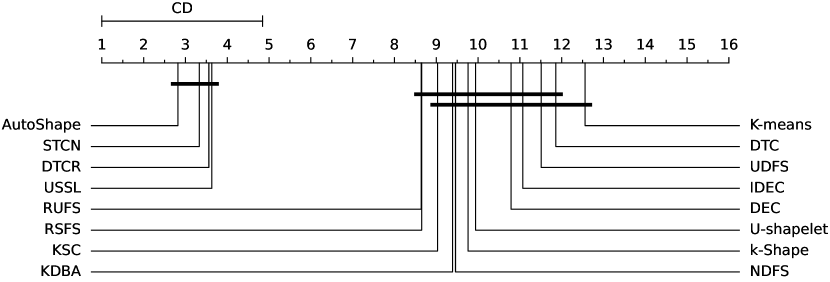
Figure 3: Critical difference diagram of the pairwise statistical comparison of $15$ methods on the $36$ datasets from UCR archive. AutoShape ranks highest among all the compared methods.

IV-C3 Varying shapelet numbers

We compare the impact of different shapelet numbers on the final NMI of AutoShape on four datasets, BirdChicken, Coffee, SwedishLeaf, and ToeSegmentation1.

Figure 4 shows the NMI by varying the shapelet numbers. Four different datasets show different trends, which guide the appropriate shapelet number of the dataset. For example, the NMI stabilizes in BirdChicken through all the different numbers of shapelet. Thus, the shapelet number of BirdChicken is $1$. The NMI rises rapidly with the increase in the shapelet number from $1$ to $20$ on SwedishLeaf, and then remains stable. Therefore, its shapelet number is set to $20$.

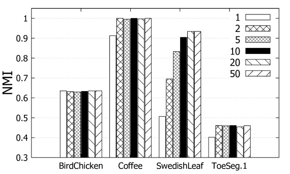
Figure 4: NMI by varying $5$ numbers of shapelet on four uts datasets

IV-C4 Ablation study

We conduct an ablation study on AutoShape to further verify the effectiveness of $\mathcal{L}_{Triplet}$, $\mathcal{L}_{Diversity}$, and $\mathcal{L}_{DBI}$. We show a comparison between the full AutoShape and its three ablation models: AutoShape without self-supervised loss (w/o triplet), AutoShape without diversity loss (w/o diversity), and AutoShape without DBI loss (w/o DBI).

We observe in Table III that all three elements make important contributions to improving the final clustering performance. The general unified representation learning (self-supervised loss) plays a particularly important role, since the NMI result of w/o triplet is always worse than the other two losses. In addition, we find that the shapelet candidates selection (diversity loss) and DBI objective clearly and consistently improve the final performance.

TABLE III: Normalized mutual information (NMI) ablation comparisons on the $36$ datasets from UCR Archive

Dataset	w/o triplet	w/o diversity	w/o DBI	AutoShape	Dataset	w/o triplet	w/o diversity	w/o DBI	AutoShape
Arrow	0.3942	0.4257	0.4344	0.5624	Mid.phal.outl.correct	0.2314	0.2534	0.2615	0.2873
Beef	0.3345	0.359	0.367	0.3799	Mid.phal.TW	0.8925	0.926	0.9307	0.945
BeetleFly	0.4894	0.5125	0.5019	0.531	MoteStrain	0.3748	0.4011	0.3924	0.4257
BirdChicken	0.541	0.6124	0.6099	0.6352	OSULeaf	0.3847	0.4127	0.4009	0.4432
Car	0.352	0.4347	0.4438	0.497	Plane	0.9045	0.985	0.972	0.9982
ChlorineConcentration	0.0095	0.0107	0.0103	0.0133	Prox.phal.outl.ageGroup	0.6051	0.6567	0.6438	0.693
Coffee	0.954	0.9854	0.9799	1	Prox.phal.TW	0.799	0.883	0.867	0.8947
DiatomsizeReduction	0.9158	0.9867	0.9943	1	SonyAIBORobotSurface	0.5048	0.5568	0.5607	0.6096
Dist.phal.outl.agegroup	0.375	0.4069	0.4168	0.44	SonyAIBORobotSurfaceII	0.6287	0.6566	0.6601	0.702
Dist.phal.outl.correct	0.099	0.1154	0.1106	0.1333	SwedishLeaf	0.843	0.9247	0.9055	0.934
ECG200	0.3048	0.3457	0.3541	0.3928	Symbols	0.8253	0.8851	0.893	0.9147
ECGFiveDays	0.714	0.756	0.769	0.7835	ToeSegmentation1	0.416	0.431	0.4301	0.461
GunPoint	0.3201	0.3652	0.3549	0.4027	ToeSegmentation2	0.4057	0.4342	0.449	0.4664
Ham	0.2563	0.294	0.305	0.3211	TwoPatterns	0.4765	0.5017	0.5102	0.515
Herring	0.1347	0.1625	0.1599	0.2019	TwoLeadECG	0.4994	0.534	0.5276	0.5654
Lighting2	0.308	0.3241	0.3197	0.353	Wafer	0.0257	0.0407	0.0398	0.052
Meat	0.882	0.9277	0.9189	0.9437	Wine	0.562	0.596	0.587	0.6045
Mid.phal.outl.agegroup	0.321	0.3467	0.3577	0.394	WordsSynonyms	0.468	0.497	0.502	0.5112

IV-C5 Comparison with other methods on RI

All the RI results of the baselines are taken from the original papers [48] and [29], respectively. The overall RI results for the $36$ UCR datasets are presented in Table IV.

From Table IV, we can observe that the overall performance of AutoShape is ranked $1st$ among all $15$ compared methods. Moreover, AutoShape performs the best in $9$ datasets, which is more than the other methods except STCN. The 1-to-1 Wins RI number of AutoShape is clearly larger than 1-to-1 Losses of all other methods. The total highest RI number of AutoShape is also larger than that of USSL and DTCR except STCN, and clearly more than those of other methods. AutoShape achieves clearly much higher RI number in some datasets, such as BirdChicken and ToeSegmentation1. Our results on 1-to-1-Losses datasets are only slightly lower than those of USSL (e.g.,  Meat, SonyAIBORobotSurface) and DTCR (e.g.,  Lighting2, Wine).

TABLE IV: Rand Index (RI) comparison on the $36$ datasets from UCR Archive

Dataset	K-means	UDFS	NDFS	RUFS	RSFS	KSC	KDBA	k-Shape	U-shapelet	DTC	USSL	DEC	IDEC	DTCR	STCN	Ours
Arrow	0.6905	0.7254	0.7381	0.7476	0.7108	0.7254	0.7222	0.7254	0.646	0.6692	0.7159	0.5817	0.621	0.6868	0.7234	0.7342
Beef	0.6713	0.6759	0.7034	0.7149	0.6975	0.7057	0.6713	0.5402	0.6966	0.6345	0.6966	0.5954	0.6276	0.8046	0.7471	0.7784
BeetleFly	0.4789	0.4949	0.5579	0.6053	0.6516	0.6053	0.6052	0.6053	0.7314	0.5211	0.8105	0.4947	0.6053	0.9	1	0.8827
BirdChicken	0.4947	0.4947	0.7316	0.5579	0.6632	0.7316	0.6053	0.6632	0.5579	0.4947	0.8105	0.4737	0.4789	0.8105	1	0.8345
Car	0.6345	0.6757	0.626	0.6667	0.6708	0.6898	0.6254	0.7028	0.6418	0.6695	0.7345	0.6859	0.687	0.7501	0.7372	0.7743
ChlorineConcentration	0.5241	0.5282	0.5225	0.533	0.5316	0.5256	0.53	0.4111	0.5318	0.5353	0.4997	0.5348	0.535	0.5357	0.5384	0.5291
Coffee	0.746	0.8624	1	0.5476	1	1	0.4851	1	1	0.4841	1	0.4921	0.5767	0.9286	1	1
DiatomsizeReduction	0.9583	0.9583	0.9583	0.9333	0.9137	1	0.9583	1	0.7083	0.8792	1	0.9294	0.7347	0.9682	0.9921	1
Dist.phal.outl.agegroup	0.6171	0.6531	0.6239	0.6252	0.6539	0.6535	0.675	0.602	0.6273	0.7812	0.665	0.7785	0.7786	0.7825	0.7825	0.7647
Dist.phal.outl.correct	0.5252	0.5362	0.5362	0.5252	0.5327	0.5235	0.5203	0.5252	0.5098	0.501	0.5962	0.5029	0.533	0.6075	0.6277	0.6258
ECG200	0.6315	0.6533	0.6315	0.7018	0.6916	0.6315	0.6018	0.7018	0.5758	0.6018	0.7285	0.6422	0.6233	0.6648	0.7081	0.7586
ECGFiveDays	0.4783	0.502	0.5573	0.502	0.5953	0.5257	0.5573	0.502	0.5968	0.5016	0.834	0.5103	0.5114	0.9638	0.6504	0.8863
GunPoint	0.4971	0.5029	0.5102	0.6498	0.4994	0.4971	0.542	0.6278	0.6278	0.54	0.7257	0.4981	0.4974	0.6398	0.7575	0.7049
Ham	0.5025	0.5219	0.5362	0.5107	0.5127	0.5362	0.5141	0.5311	0.5362	0.5648	0.6393	0.5963	0.4956	0.5362	0.5879	0.6543
Herring	0.4965	0.5099	0.5164	0.5238	0.5151	0.494	0.5164	0.4965	0.5417	0.5045	0.619	0.5099	0.5099	0.5759	0.6036	0.6286
Lighting2	0.4966	0.5119	0.5373	0.5729	0.5269	0.6263	0.5119	0.6548	0.5192	0.577	0.6955	0.5311	0.5519	0.5913	0.6786	0.7205
Meat	0.6595	0.6483	0.6635	0.6578	0.6657	0.6723	0.6816	0.6575	0.6742	0.322	0.774	0.6475	0.622	0.9763	0.9186	0.9257
Mid.phal.outl.agegroup	0.5351	0.5269	0.535	0.5315	0.5473	0.5364	0.5513	0.5105	0.5396	0.5757	0.5807	0.7059	0.68	0.7982	0.7975	0.7538
Mid.phal.outl.correct	0.5	0.5431	0.5047	0.5114	0.5149	0.5014	0.5563	0.5114	0.5218	0.5272	0.6635	0.5423	0.5423	0.5617	0.5442	0.6524
Mid.phal.TW	0.0983	0.1225	0.1919	0.792	0.8062	0.8187	0.8046	0.6213	0.792	0.7115	0.792	0.859	0.8626	0.8638	0.8625	0.7724
MoteStrain	0.4947	0.5579	0.6053	0.5579	0.6168	0.6632	0.4789	0.6053	0.4789	0.5062	0.8105	0.7435	0.7324	0.7686	0.656	0.7958
OSULeaf	0.5615	0.5372	0.5622	0.5497	0.5665	0.5714	0.5541	0.5538	0.5525	0.7329	0.6551	0.7484	0.7607	0.7739	0.7615	0.6425
Plane	0.9081	0.8949	0.8954	0.922	0.9314	0.9603	0.9225	0.9901	1	0.904	1	0.9447	0.9447	0.9549	0.9663	1
Prox.phal.outl.ageGroup	0.5288	0.4997	0.5463	0.578	0.5384	0.5305	0.5192	0.5617	0.5206	0.743	0.7939	0.4263	0.8091	0.8091	0.8379	0.7849
Prox.phal.TW	0.4789	0.4947	0.6053	0.5579	0.5211	0.6053	0.5211	0.5211	0.4789	0.838	0.7282	0.8189	0.903	0.9023	0.8984	0.7049
SonyAIBORobotSurface	0.7721	0.7695	0.7721	0.7787	0.7928	0.7726	0.7988	0.8084	0.7639	0.5563	0.8105	0.5732	0.69	0.8769	0.7356	0.8954
SonyAIBORobotSurfaceII	0.8697	0.8745	0.8865	0.8756	0.8948	0.9039	0.8684	0.5617	0.877	0.7012	0.8575	0.6514	0.6572	0.8354	0.7417	0.8987
SwedishLeaf	0.4987	0.4923	0.55	0.5192	0.5038	0.4923	0.55	0.5333	0.6154	0.8871	0.8547	0.8837	0.8893	0.9223	0.8872	0.9018
Symbols	0.881	0.8548	0.8562	0.8525	0.906	0.8982	0.9774	0.8373	0.9603	0.9053	0.92	0.8841	0.8857	0.9168	0.9088	0.9119
ToeSegmentation1	0.4873	0.4921	0.5873	0.5429	0.4968	0.5	0.6143	0.6143	0.5873	0.5077	0.6718	0.4984	0.5017	0.5659	0.8177	0.7041
ToeSegmentation2	0.5257	0.5257	0.5968	0.5968	0.5826	0.5257	0.5573	0.5257	0.502	0.5348	0.6778	0.4991	0.4991	0.8286	0.8186	0.8546
TwoPatterns	0.8529	0.8259	0.853	0.8385	0.8588	0.8585	0.8446	0.8046	0.7757	0.6251	0.8318	0.6293	0.6338	0.6984	0.7619	0.8217
TwoLeadECG	0.5476	0.5495	0.6328	0.8246	0.5635	0.5464	0.5476	0.8246	0.5404	0.5116	0.8628	0.5007	0.5016	0.7114	0.9486	0.8556
Wafer	0.4925	0.4925	0.5263	0.5263	0.4925	0.4925	0.4925	0.4925	0.4925	0.5324	0.8246	0.5679	0.5597	0.7338	0.8433	0.8094
Wine	0.4984	0.4987	0.5123	0.5021	0.5033	0.5006	0.5064	0.5001	0.5033	0.4906	0.8985	0.4913	0.5157	0.6271	0.6925	0.8814
WordsSynonyms	0.8775	0.8697	0.876	0.8861	0.8817	0.8727	0.8159	0.7844	0.823	0.8855	0.854	0.8893	0.8947	0.8984	0.8748	0.8641
Rank	12.5	11.53	8.97	9.11	8.63	8.82	9.67	10.06	9.99	10.65	4.72	10.43	9.26	4.17	3.94	3.56
Total best acc	0	0	1	1	1	4	1	2	2	0	7	0	1	8	11	9
Ours 1-to-1 Wins	34	34	32	31	31	30	32	31	33	32	20	31	30	23	20	-
Ours 1-to-1 Draws	0	0	1	0	1	2	0	2	1	0	3	0	0	0	1	-
Ours 1-to-1 Losses	2	2	3	5	4	4	4	3	2	4	13	5	6	13	15	-
Wilcoxon P-value	0	0	0	0	0	0	0	0	0	0	0.002	0	0	0.049	0.612	-

IV-C6 Network comparison

We compare the performance of using Temporal Convolutional Network (TCN) [4] and a recurrent network (e.g.,  vanilla RNN [46]) for an autoencoder.

We show a comparison between the TCN and vanilla RNN on the final NMI (in Figure 5(a)) and RI (in Figure 5(b)) performance. The final result shows that the differences in NMI and RI between TCN and vanilla RNN are negligible in most datasets. The statistical test reveals no evidence that either network is better than the other. The network obey causal ordering (i.e.,  no future value impacts the current value) is the only requirement.

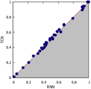
(a) Comparison on NMI

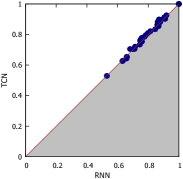
(b) Comparison on RI

Figure 5: (a) The comparison of TCN and vanilla RNN over 36 datasets on NMI; and (b) The comparison of TCN and vanilla RNN over 36 datasets on RI. The dots above the diagonal indicate datasets over which TCN has better performance than vanilla RNN; vanilla RNN performs better, otherwise.

IV-C7 Experiments on uts interpretability

We further investigate the interpretability of the shapelets, which is a strength of shapelet-based methods. We report the shapelets ($k$ =1, 2) generated by AutoShape from two datasets. These datasets are chosen simply because they can be presented without much domain knowledge. From Figures 6 and 7,we can observe that some subsequences of the original time series of the clusters are similar to their shapelets, which is the reason why they are clustered.

Case study 1: ToeSegmentation1. The ToeSegmentation1 dataset [7] is the left toe of z-axis value of human gait recognition (first used in [44]) derived from CMU Graphics Lab Motion Capture Database(CMU). The dataset consists of two categories, “normal walk” and “abnormal walk” containing hobble walk, hurt leg walk and others. In the abnormal walk category, the actors are pretending to have difficulty walking normally.

From Figure 6, we can easily find that the top-2 shapelets $S_{1}$ and $S_{2}$ are more frequent in normal walk class. $S_{1}$ shows one unit of normal walk and $S_{2}$ presents the interval of two consecutive walk units.

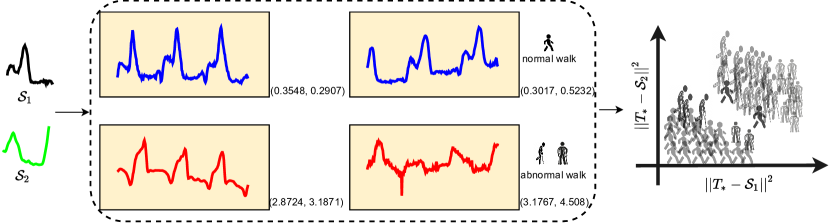
Figure 6: The top-2 shapelets $S_{1}$ and $S_{2}$ (leftmost plots) are discovered from the ToeSegmentation1 dataset by AutoShape. The middle plots show four time series instances from two classes of the dataset. Different colors show different classes (blue for normal walk and red for abnormal walk). The distances to the shapelets and the original time series are used to project them into a 2-dimensional space (rightmost plot).

Case study 2: ItalyPowerDemand. ItalyPowerDemand [7] was derived from $12$ monthly electrical power consumption time series from Italy in 1997. Two classes are in the dataset, summer from April to September, winter from October to March.

$S_{1}$ is learned by AutoShape showed in the left part of Figure 7. From the learned shapelet, we can identify that the power demand in summer is lower than that in winter from 5am to 11pm. This is because the heating in the morning used during the winter time and air conditioning in summer was still fairly rare in Italy when the data were collected.

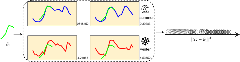
Figure 7: An example of shapelet transformation on ItalyPowerDemand. The original time series from summer class (blue) and winter class (red) are displayed in the middle. We can cluster the transformed representations into two classes effectively.

IV-D Experiments on multivariate time series

Next, we highlight the major results from the experiments conducted on mts. We take NMI [48] as the metric for evaluating the methods on mts. We omit the rand index (RI) results, as they exhibit similar trends. We choose K-means, GMM, k-Shape, USSL and DTCR as the compared methods . Since they do not consider mts datasets, we simply concatenate the different variables into one variable for the mts version (e.g., k-Shape-M, USSL-M, and DTCR-M). The results of all $6$ methods are the mean values of $10$ runs and the standard deviations of all the datasets are less than $0.01$.

IV-D1 NMI on multivariate time series

The overall NMI results for the 30 UEA mts datasets are presented in Table V.

From Table V, we can observe that the overall performance of AutoShape ranks first among all the $6$ compared methods. Moreover, AutoShape performs the best in $22$ mts datasets, which is significantly more than the other $5$ methods. The results show that AutoShape can learn the shapelets of high quality from different variables.

TABLE V: Normalized mutual information (NMI) comparison on the UEA Archive

Dataset	K-means	GMM	k-Shape-M	USSL-M	DTCR-M	AutoShape
ArticularyWordRecognition	0.91	0.92	0.90	0.40	0.83	0.93
AtrialFibrillation	0.00	0.00	0.33	0.44	0.23	0.50
BasicMotions	0.05	0.00	0.94	0.40	0.50	0.55
CharacterTrajectories	0.72	0.51	0.79	0.50	0.52	0.71
Cricket	0.80	0.88	0.96	0.79	0.84	0.85
DuckDuckGeese	0.04	0.04	0.25	0.31	0.32	0.35
EigenWorms	0.05	0.04	0.22	0.35	0.36	0.42
Epilepsy	0.30	0.25	0.37	0.40	0.20	0.42
ERing	0.35	0.33	0.30	0.31	0.36	0.37
EthanolConcentration	0.02	0.01	0.01	0.10	0.05	0.14
FaceDetection	0.00	0.00	0.00	0.06	0.05	0.18
FingerMovements	0.02	0.00	0.01	0.02	0.01	0.04
HandMovementDirection	0.02	0.04	0.10	0.10	0.08	0.18
Handwriting	0.24	0.23	0.48	0.44	0.46	0.51
Heartbeat	0.01	0.00	0.04	0.05	0.07	0.10
InsectWingbeat	0.01	0.03	0.06	0.09	0.10	0.10
JapaneseVowels	0.72	0.63	0.75	0.67	0.47	0.72
Libras	0.62	0.49	0.62	0.61	0.63	0.66
LSST	0.03	0.00	0.22	0.20	0.26	0.28
MotorImagery	0.01	0.01	0.01	0.02	0.08	0.10
NATOPS	0.57	0.55	0.57	0.55	0.28	0.58
PEMS-SF	0.33	0.36	0.36	0.41	0.46	0.43
PenDigits	0.66	0.75	0.17	0.68	0.47	0.70
Phoneme	0.15	0.08	0.17	0.21	0.24	0.24
RacketSports	0.37	0.15	0.51	0.51	0.27	0.46
SelfRegulationSCP1	0.12	0.00	0.18	0.55	0.11	0.58
SelfRegulationSCP2	0.00	0.00	0.001	0.58	0.00	0.60
SpokenArabicDigits	0.70	0.17	0.88	0.29	0.22	0.45
StandWalkJump	0.00	0.00	0.18	0.51	0.23	0.52
UWaveGestureLibrary	0.68	0.67	0.55	0.69	0.25	0.71
Total best acc	0	1	6	1	3	22
Ours 1-to-1 Wins	27	29	24	29	27	-
Ours 1-to-1 Draws	1	0	0	0	1	-
Ours 1-to-1 Losses	2	1	6	1	2	-

IV-D2 Friedman test and wilcoxon test

Again, we follow the process described in [9] to do the Friedman test and the Wilcoxon-signed rank test with Holm’s $\alpha$ ($5$%) [17].

The Friedman test is used to detect the differences in $30$ UEA datasets across $6$ methods. Our statistical significance is $p<0.001$, which is smaller than $\alpha=0.05$. Thus, we reject the null hypothesis, and there is a significant difference among all $6$ methods.

We then conduct the post-hoc analysis among all the compared methods. The results are visualized by the critical difference diagram in Figure 8. We can clearly note that AutoShape outperforms all other $5$ methods significantly.

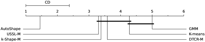
Figure 8: Critical difference diagram of the pairwise statistical comparison of $6$ methods on the UEA archive. AutoShape outperforms all other $5$ methods significantly

IV-D3 Varying shapelet numbers

We further compare the impact of different shapelet numbers on the final NMI of AutoShape on four mts datasets, BasicMotions, Epilepsy, SelfRegulationSCP1, and StandWalkJump.

Figure 9 presents NMI by varying the $6$ different shapelet numbers. Four different datasets exhibit different trends, which show the appropriate shapelet number selection for the dataset. For example, NMI increases rapidly with the increase in the shapelet number from $1$ to $2$ on Epilepsy, and then remains stable. Thus, its shapelet number is set to $2$.

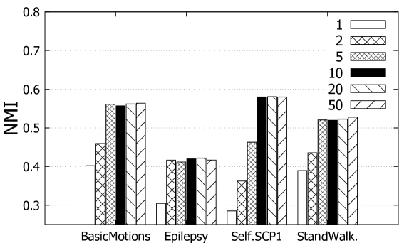
Figure 9: NMI by varying $5$ numbers of shapelet on four mts datasets

IV-D4 Experiments on mts interpretability

Finally, we investigate the interpretability of the learned shapelets on mts. We describe the shapelets (e.g.,  $k$ = 2) generated by AutoShape from the Epilepsy dataset [3] in Figures 10. Again, we choose the dataset simply because it can be illustrated without much domain knowledge. The Epilepsy dataset was generated with healthy participants simulating the class activities performed. The dataset consists of $4$ categories, “walking”, “running”, “sawing” and “seizure mimicking”.

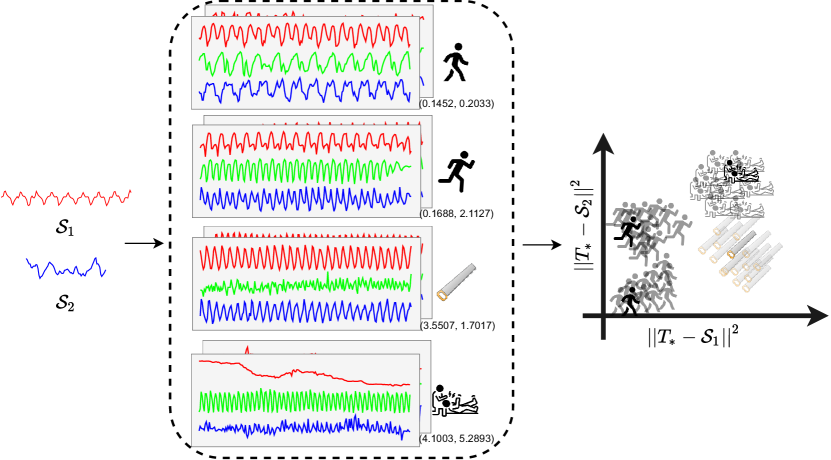
Figure 10: The top-2 shapelets $S_{1}$ and $S_{2}$ are learned from the Epilepsy dataset (leftmost plots) by AutoShape. The middle plots show the time series instances from four classes. Three different colors show the different variables. The original time series are projected into a 2-dimensional space (rightmost plot). Most of the original time series can be correctly clustered.

V Conclusion

This paper has proposed a novel autoencoder-based shapelet approach for time series clustering, called AutoShape. We propose an autoencoder network to learn the unified embeddings of shapelet candidates via the following objectives. Self-supervised loss is for learning the general embedding of time series subsequences (shapelet candidates). We propose diversity loss among shapelet candidates to select diverse candidates. The reconstruction loss maintains the original time series’ shapes for interpretability. DBI is an internal index to guide network learning for improving clustering performance. Extensive experiments show the superiority of our AutoShape to the other $14$ and $5$ compared methods on uts and mts datasets, respectively. The interpretability of the learned shapelets is illustrated with three case studies on the UCR uts datasets and one case study on the UEA mts datasets. As for the future work, we plan to study the efficiency and the missing values in shapelet-based methods for tsc.

Guozhong Li is a Post-doctoral Research Fellow in the Department of Computer Science, Hong Kong Baptist University. He received the Ph.D. degree in computer science from Hong Kong Baptist University, HKSAR, China, in 2021. His research interests include time series analysis, neural networking, and graph mining. He is a member of the Database Group at Hong Kong Baptist University (http://www.comp.hkbu.edu.hk/$\sim$db/).

Byron Choi is an Associate Professor in the Department of Computer Science at the Hong Kong Baptist University. He received the bachelor of engineering degree in computer engineering from the Hong Kong University of Science and Technology (HKUST) in 1999 and the MSE and PhD degrees in computer and information science from the University of Pennsylvania in 2002 and 2006, respectively.

Jianliang Xu is a Professor in the Department of Computer Science, Hong Kong Baptist University (HKBU). He held visiting positions at Pennsylvania State University and Fudan University. He has published more than 150 technical papers in these areas, most of which appeared in leading journals and conferences including SIGMOD, VLDB, ICDE, TODS, TKDE, and VLDBJ.

Sourav S Bhowmick is an Associate Professor in the School of Computer Science and Engineering, Nanyang Technological University. Sourav’s current research interests include data management, data analytics, computational social science, and computational systems biology. He has published many papers in major venues in these areas such as SIGMOD, VLDB, ICDE, SIGKDD, MM, TKDE, VLDB Journal, and Bioinformatics.

Daphne Ngar-yin Mah is Director of Asian Energy Studies Centre, and Associate Professor at Department of Geography at Hong Kong Baptist University. Her research focuses on social aspects of smart energy transitions, specialising in interdisciplinary research that cuts across the fields of energy technologies (smart grids, solar power, wind energy, nuclear power, and building energy efficiency), energy governance, and sustainability policy studies, with a geographical focus on East Asia covering empirical cases in China, South Korea, and Japan.

Grace L.H.Wong is a Professor in the Department of Medicine & Therapeutics, Consultant Hepatologist, Center for Liver Health, The Chinese University of Hong Kong. Dr. Grace Wong has published over 160 articles in peer-reviewed journals including Gastroenterology, Hepatology and Gut. She is currently a reviewer of 44 biomedical journals, the editorial board members of 5 journals and associate editor of Journal of Gastroenterology and Hepatology.

References

- [1] S. Aghabozorgi, A. S. Shirkhorshidi, and T. Y. Wah. Time-series clustering–a decade review. Information Systems, 53:16–38, 2015.
- [2] N. Asadi, A. Mirzaei, and E. Haghshenas. Creating discriminative models for time series classification and clustering by hmm ensembles. IEEE Transactions on Cybernetics, 46(12):2899–2910, 2016.
- [3] A. Bagnall, H. A. Dau, J. Lines, M. Flynn, J. Large, A. Bostrom, P. Southam, and E. Keogh. The uea multivariate time series classification archive, 2018. arXiv preprint arXiv:1811.00075, 2018.
- [4] S. Bai, J. Z. Kolter, and V. Koltun. An empirical evaluation of generic convolutional and recurrent networks for sequence modeling. arXiv preprint arXiv:1803.01271, 2018.
- [5] D. Bertsimas, A. Orfanoudaki, and H. Wiberg. Interpretable clustering: an optimization approach. Machine Learning, 110(1):89–138, 2021.
- [6] S. Boyd and L. Vandenberghe. Convex optimization. Cambridge university press, 2004.
- [7] H. A. Dau, E. Keogh, K. Kamgar, C.-C. M. Yeh, Y. Zhu, S. Gharghabi, C. A. Ratanamahatana, Yanping, B. Hu, N. Begum, A. Bagnall, A. Mueen, and G. Batista. The ucr time series classification archive, October 2018. https://www.cs.ucr.edu/~eamonn/time_series_data_2018/.
- [8] D. L. Davies and D. W. Bouldin. A cluster separation measure. IEEE Transactions on Pattern Analysis and Machine Intelligence, (2):224–227, 1979.
- [9] J. Demšar. Statistical comparisons of classifiers over multiple data sets. Journal of Machine Learning Research, 7(Jan):1–30, 2006.
- [10] Z. Fang, P. Wang, and W. Wang. Efficient learning interpretable shapelets for accurate time series classification. In 2018 IEEE 34th International Conference on Data Engineering (ICDE), pages 497–508, 2018.
- [11] J. Grabocka, N. Schilling, M. Wistuba, and L. Schmidt-Thieme. Learning time-series shapelets. In Proceedings of the 20th ACM SIGKDD, pages 392–401, 2014.
- [12] H. Guo, L. Wang, X. Liu, and W. Pedrycz. Information granulation-based fuzzy clustering of time series. IEEE Transactions on Cybernetics, 51(12):6253–6261, 2021.
- [13] H. Guo, L. Wang, X. Liu, and W. Pedrycz. Trend-based granular representation of time series and its application in clustering. IEEE Transactions on Cybernetics, 2021.
- [14] X. Guo, L. Gao, X. Liu, and J. Yin. Improved deep embedded clustering with local structure preservation. In The international joint conference on artificial intelligence (IJCAI), pages 1753–1759, 2017.
- [15] J. A. Hartigan and M. A. Wong. Algorithm as 136: A k-means clustering algorithm. Journal of the royal statistical society. series c (applied statistics), 28(1):100–108, 1979.
- [16] G. He, H. Wang, S. Liu, and B. Zhang. Csmvc: A multiview method for multivariate time-series clustering. IEEE Transactions on Cybernetics, 2021.
- [17] S. Holm. A simple sequentially rejective multiple test procedure. Scandinavian journal of statistics, pages 65–70, 1979.
- [18] L. Hou, J. T. Kwok, and J. M. Zurada. Efficient learning of timeseries shapelets. In Proceedings of the AAAI Conference on Artificial Intelligence, pages 1209–1215, 2016.
- [19] E. L. Lehmann and G. Casella. Theory of point estimation. Springer Science & Business Media, 2006.
- [20] G. Li, B. Choi, J. Xu, S. S. Bhowmick, K. P. Chun, and G. Wong. Shapenet: A shapelet-neural network approach for multivariate time series classification. Proceedings of the AAAI Conference on Artificial Intelligence, 2021.
- [21] G. Li, B. Choi, J. Xu, S. S. Bhowmick, K. P. Chun, and G. Wong. Efficient shapelet discovery for time series classification. IEEE Transactions on Knowledge and Data Engineering, 34(3):1149–1163, 2022.
- [22] H. Li. Multivariate time series clustering based on common principal component analysis. Neurocomputing, 349:239–247, 2019.
- [23] X.-H. Li, C. C. Cao, Y. Shi, W. Bai, H. Gao, L. Qiu, C. Wang, Y. Gao, S. Zhang, X. Xue, et al. A survey of data-driven and knowledge-aware explainable ai. IEEE Transactions on Knowledge and Data Engineering, 34(1):29–48, 2022.
- [24] Z. Li, Y. Yang, J. Liu, X. Zhou, and H. Lu. Unsupervised feature selection using nonnegative spectral analysis. In Proceedings of the AAAI Conference on Artificial Intelligence, 2012.
- [25] T. W. Liao. Clustering of time series data—a survey. Pattern recognition, 38(11):1857–1874, 2005.
- [26] J. Lin, E. Keogh, S. Lonardi, and B. Chiu. A symbolic representation of time series, with implications for streaming algorithms. In Proceedings of the 8th ACM SIGMOD workshop on Research issues in data mining and knowledge discovery, pages 2–11, 2003.
- [27] J. Lines, L. M. Davis, J. Hills, and A. Bagnall. A shapelet transform for time series classification. In Proceedings of the 18th ACM SIGKDD, pages 289–297, 2012.
- [28] Q. Ma, S. Li, W. Zhuang, J. Wang, and D. Zeng. Self-supervised time series clustering with model-based dynamics. IEEE Transactions on Neural Networks and Learning Systems, 32(9):3942–3955, 2021.
- [29] Q. Ma, J. Zheng, S. Li, and G. W. Cottrell. Learning representations for time series clustering. In Advances in Neural Information Processing Systems, pages 3781–3791, 2019.
- [30] N. S. Madiraju, S. M. Sadat, D. Fisher, and H. Karimabadi. Deep temporal clustering: Fully unsupervised learning of time-domain features. arXiv preprint arXiv:1802.01059, 2018.
- [31] A. Mueen, E. Keogh, and N. Young. Logical-shapelets: an expressive primitive for time series classification. In Proceedings of the 17th ACM SIGKDD, pages 1154–1162, 2011.
- [32] J. Paparrizos and L. Gravano. k-shape: Efficient and accurate clustering of time series. In Proceedings of the SIGMOD, pages 1855–1870, 2015.
- [33] F. Petitjean, A. Ketterlin, and P. Gançarski. A global averaging method for dynamic time warping, with applications to clustering. Pattern Recognition, 44(3):678–693, 2011.
- [34] M. Qian and C. Zhai. Robust unsupervised feature selection. In The international joint conference on artificial intelligence (IJCAI), 2013.
- [35] O. Rippel, M. Paluri, P. Dollar, and L. Bourdev. Metric learning with adaptive density discrimination. 2016 International Conference on Learning Representations, 2016.
- [36] F. Schroff, D. Kalenichenko, and J. Philbin. Facenet: A unified embedding for face recognition and clustering. In Proceedings of the IEEE CVPR, pages 815–823, 2015.
- [37] L. Shi, L. Du, and Y.-D. Shen. Robust spectral learning for unsupervised feature selection. In 2014 IEEE 14th International Conference on Data Mining (ICDM), pages 977–982, 2014.
- [38] A. Singhal and D. E. Seborg. Clustering multivariate time-series data. Journal of Chemometrics: A Journal of the Chemometrics Society, 19(8):427–438, 2005.
- [39] L. Ulanova, N. Begum, and E. Keogh. Scalable clustering of time series with u-shapelets. In Proceedings of the 2015 SIAM International Conference on Data Mining, pages 900–908, 2015.
- [40] J. Xie, R. Girshick, and A. Farhadi. Unsupervised deep embedding for clustering analysis. In International conference on machine learning, pages 478–487, 2016.
- [41] J. Yang and J. Leskovec. Patterns of temporal variation in online media. In Proceedings of the fourth ACM international conference on Web search and data mining, pages 177–186, 2011.
- [42] Y. Yang, H. T. Shen, Z. Ma, Z. Huang, and X. Zhou. L2, 1-norm regularized discriminative feature selection for unsupervised. In The International Joint Conference on Artificial Intelligence (IJCAI), 2011.
- [43] L. Ye and E. Keogh. Time series shapelets: a new primitive for data mining. In Proceedings of the 15th ACM SIGKDD, pages 947–956, 2009.
- [44] L. Ye and E. Keogh. Time series shapelets: a novel technique that allows accurate, interpretable and fast classification. Data Mining and Knowledge Discovery, 22(1-2):149–182, 2011.
- [45] C.-C. M. Yeh, Y. Zhu, L. Ulanova, N. Begum, Y. Ding, H. A. Dau, D. F. Silva, A. Mueen, and E. Keogh. Matrix profile i: all pairs similarity joins for time series: a unifying view that includes motifs, discords and shapelets. In 2016 IEEE 16th International Conference on Data Mining (ICDM), pages 1317–1322, 2016.
- [46] J. Yoon, D. Jarrett, and M. van der Schaar. Time-series generative adversarial networks. In Advances in Neural Information Processing Systems, pages 5508–5518, 2019.
- [47] J. Zakaria, A. Mueen, and E. Keogh. Clustering time series using unsupervised-shapelets. In 2012 IEEE 12th International Conference on Data Mining (ICDM), pages 785–794, 2012.
- [48] Q. Zhang, J. Wu, P. Zhang, G. Long, and C. Zhang. Salient subsequence learning for time series clustering. IEEE Transactions on Pattern Analysis and Machine Intelligence, 41(9):2193–2207, 2019.
- [49] P.-Y. Zhou and K. C. Chan. A model-based multivariate time series clustering algorithm. In Pacific-Asia Conference on Knowledge Discovery and Data Mining, pages 805–817. Springer, 2014.