Enumeration of connected bipartite graphs with given Betti number

Abstract.

We obtain first order linear partial differential equations which are satisfied by exponential generating functions of two variables for the number of connected bipartite graphs with given Betti number. By solving these equations inductively, we obtain the explicit form of generating functions and derive the asymptotic behavior of their coefficients. We also introduce a family of basic graphs to classify connected bipartite graphs and give another expression of the generating functions as the sum over basic graphs of rational functions of those for the number of labeled bipartite rooted spanning trees.

1. Introduction

Let $G=(V,E)$ be a simple graph, i.e., no self-loops and multiple edges, and we call it an $(n,q)$-graph if $|V|=n$ and $|E|=q$. We denote the number of connected graphs with $k$ independent cycles, by $N(n,k)$, which is also equal to the number of connected $(n,n-1+k)$-graphs. Since we are dealing with connected graphs, we note that $k$ corresponds to the Betti number, the rank of the first homology group, of each $(n,n-1+k)$-graph. Note that $k-1$ is often called excess since such a connected graph has $k-1$ more edges than vertices. Connected $(n,n-1)$-graphs are spanning trees in the complete graph $K_{n}$ over $n$ vertices and it is known as Cayley’s formula [1] that $N(n,0)=n^{n-2}$. Connected $(n,n)$-graphs are called unicycles and the formula for $N(n,1)$ was found by Rényi [9], which is given by

$$N(n,1)=\frac{1}{2}\left(\frac{h(n)}{n}-n^{n-2}(n-1)\right)\sim\sqrt{\frac{\pi}{8}}n^{n-1/2}\quad(n\to\infty),$$ (1.1)

where

$$h(n)=\sum_{s=1}^{n-1}{n\choose s}s^{s}(n-s)^{n-s}.$$

The asymptotic behavior of $N(n,k)$ for general $k$ as $n\to\infty$ was also discussed in [12], where the proofs are based on recurrence equations which $N(n,k)$’s satisfy, the algebraic structures of generating functions and their derivatives, and the combinatorial aspect as will be seen in Theorem 1.6 below.

We consider a bipartite simple graph $G=(V,E)$ with bipartition $V=V_{1}\sqcup V_{2}$ and call it a bipartite $(r,s,q)$-graph if $|V_{1}|=r$, $|V_{2}|=s$ and $|E|=q$, which is also considered as a connected spanning subgraph with $q$-edges in the bipartite graph $K_{r,s}$. We denote by $N_{{\rm bi}}(r,s,k)$ the number of connected bipartite $(r,s,r+s+k-1)$-graphs, whose Betti number is $k$. Similarly as before, connected bipartite $(r,s,r+s-1)$-graphs are spanning trees in $K_{r,s}$ and it is well known [11] that

$$N_{{\rm bi}}(r,s,0)=r^{s-1}s^{r-1},$$ (1.2)

which is the bipartite version of Cayley’s formula.

When $rs=0$, we understand $N_{{\rm bi}}(r,s,0)=1$ if $(r,s)=(1,0),(0,1)$; $=0$ otherwise, i.e., the one-vertex simple graph is regarded as a spanning tree. Connected bipartite $(r,s,r+s)$-graphs are unicycles in $K_{r,s}$ and discussed in the context of cuckoo hushing by [8]. In the present paper, we discuss $N_{{\rm bi}}(r,s,k)$ for $k=0,1,\dots$ and the asymptotic behavior of sum of $N_{{\rm bi}}(r,s,k)$ with $r+s=n$.

We consider the exponential generating function of $N_{{\rm bi}}(r,s,k)$ defined as follows: for $k=0,1,\dots$,

$$F_{k}(x,y):=\sum_{r,s=0}^{\infty}\frac{N_{{\rm bi}}(r,s,k)}{r!s!}x^{r}y^{s}.$$ (1.3)

For simplicity, we write the exponential generating function for spanning trees in (1.2) by

$$T(x,y):=F_{0}(x,y)=x+y+\sum_{r,s=1}^{\infty}\frac{r^{s-1}s^{r-1}}{r!s!}x^{r}y^{s}.$$ (1.4)

We introduce the following functions of $x$ and $y$:

$$T_{x}=D_{x}T,\quad T_{y}=D_{y}T,\quad Z=T_{x}+T_{y},\quad W=T_{x}T_{y},$$ (1.5)

where $D_{x}=x\partial_{x}$ and $D_{y}=y\partial_{y}$ are the Euler differential operators. Then we have the following.

Proposition 1.1.

The function $F_{1}(x,y)$ is expressed as $F_{1}=f_{1}(W)$ with $f_{1}(w)=-\frac{1}{2}\big{(}\log(1-w)+w\big{)}$, i.e.,

$$F_{1}(x,y)=-\frac{1}{2}\Big{(}\log(1-T_{x}T_{y})+T_{x}T_{y}\Big{)}.$$

This result was discussed in (cf. [8, Lemma 4.4],[2]). However, the term $w$ seems missing in $f_{1}(w)$ and $F_{1}(x,y)$ was given as $-\frac{1}{2}\log(1-T_{x}T_{y})$, which does not give integer coefficients.

We will give how to compute $F_{k}(x,y)$ for general $k$ later and, in principle, we are able to compute them inductively. Here, we just give the expression $F_{2}(x,y)$ (see Remark 3.3 for $F_{3}(x,y)$ and $F_{4}(x,y)$).

Theorem 1.2.

The function $F_{2}(x,y)$ is expressed as $F_{2}=f_{2}(Z,W)$ with

$$f_{2}(z,w)=\frac{w^{2}}{24(1-w)^{3}}\big{\{}(2+3w)z+2w(6-w)\big{\}}.$$ (1.6)

From Proposition 1.1 and Theorem 1.2, the asymptotic behavior for coefficients of the diagonals $F_{1}(x,x)$ and $F_{2}(x,x)$ is derived as follows. Let $\langle x^{n}\rangle A(x)$ denote the operation of extracting the coefficient $a_{n}$ of $x^{n}/n!$ in an exponential formal power series $A(x)=\sum_{n=0}^{\infty}a_{n}\frac{x^{n}}{n!}$, i.e.

$$\langle x^{n}\rangle A(x)=a_{n}.$$ (1.7)

The coefficients of $\langle x^{n}\rangle F_{k}(x,x)$ counts the number of connected bipartite graphs with Betti number $k$ over $n$ vertices, or equivalently, the total number of connected bipartite $(r,s,n-1+k)$-graphs with $r+s=n$. For convenience, we denote it by

$$N_{{\rm bi}}(n,k):=\langle x^{n}\rangle F_{k}(x,x)=\sum_{r+s=n}\binom{n}{r}N_{{\rm bi}}(r,s,k).$$ (1.8)

When $k=0$, we have

$$F_{0}(x,x)=2\Big{(}x+\sum_{n=2}^{\infty}n^{n-2}\frac{x^{n}}{n!}\Big{)},$$

hence $N_{{\rm bi}}(n,0)=2n^{n-2}=2N(n,0)$, which is equivalent to (4.4). That is, as we will see in Section 4, the spanning trees in $K_{r,s}$ for some $(r,s)$ with $r+s=n$ are in two-to-one correspondence with those in $K_{n}$. When $k\geq 1$, the situation is different since there may exist cycles having odd length in $K_{n}$ while cycles must have even length in $K_{r,s}$. From Proposition 1.1 and Theorem 1.2, we obtain the asymptotic behavior of $N_{{\rm bi}}(n,1)$ and $N_{{\rm bi}}(n,2)$.

Theorem 1.3.

For $n=4,5,\dots$,

$$N_{{\rm bi}}(n,1)=n^{n-1}\sum_{2\leq k\leq n/2}\dfrac{n!}{(n-2k)!n^{2k}}\sim\sqrt{\dfrac{\pi}{8}}n^{n-1/2}\quad(n\to\infty).$$

$n$	3	4	5	6	7	8	9	10	11
$N(n,1)$	1	15	222	3660	68295	1436568	33779340	880107840	25201854045
$N_{{\rm bi}}(n,1)$	0	6	120	2280	46200	1026840	25102224	673706880	19745850960

Figure 1. $N(n,1)$ and $N_{{\rm bi}}(n,1)$ for $n=3,4,\dots,11$

From (1.1), this shows that the main term of the asymptotic behavior of the number of bipartite unicycles over $n$ vertices is the same as that of the number of unicycles.

Theorem 1.4.

As $n\to\infty$,

$$N_{{\rm bi}}(n,2)\sim\frac{5}{48}n^{n+1}.$$ (1.9)

It is known [12] that in the case of $K_{n}$, the main term of asymptotic behavior of the number of “bicycles” is known to be $\frac{5}{24}n^{n+1}$, which is twice of (1.9).

$n$	4	5	6	7	8	9	10	11
$N(n,2)$	6	205	5700	156555	4483360	136368414	4432075200	154060613850
$N_{{\rm bi}}(n,2)$	0	20	960	33600	1111040	37202760	1295884800	47478243120

Figure 2. $N(n,2)$ and $N_{{\rm bi}}(n,2)$ for $n=4,5,\dots,11$

For general $k$, we have the following asymptotic equality.

Theorem 1.5.

For $k\geq 0$, as $n\to\infty$,

$$N_{{\rm bi}}(n,k)\sim\frac{1}{2^{k-1}}N(n,k).$$ (1.10)

The proof of (1.10) is given in Section 6. The following asymptotic behavior

$$N(n,k)\sim\rho_{k-1}n^{n+(3k-4)/2}\quad(n\to\infty)$$

is given in [12], where the explicit value of $\rho_{k}$ can be computed by the recurrence equation. Comparing the generating function of [12, Section 8] with that of this paper, we can see that the subscript $k$ is off by one. However, the meaning of both is the same. To derive (1.10), we use the following result, which would be interesting on its own right and give more detailed information.

Theorem 1.6.

For $k\geq 2$, $F_{k}(x,y)$ is decomposed into the sum of rational functions of $T_{x}$ and $T_{y}$ over the set $BG_{k}$ of basic graphs with Betti number $k$ as

$$F_{k}(x,y)=\sum_{\mathcal{B}\in BG_{k}}J_{\mathcal{B}}(x,y)$$ (1.11)

with

$$J_{\mathcal{B}}(x,y)=\frac{T_{x}^{|V_{1}|}T_{y}^{|V_{2}|}}{g_{\mathcal{B}}(1-T_{x}T_{y})^{N_{\rm sp}+k-1-e}}$$ (1.12)

where $V_{1}\sqcup V_{2}$ is the vertex set of $\mathcal{B}$, $g_{\mathcal{B}}$ is the number of automorphisms of $\mathcal{B}$, $N_{\rm sp}$ and $e$ are the numbers of vertices with degree $\geq 3$ and $\delta$-edges in $\mathcal{B}$, respectively.

The definitions of basic graph and $\delta$-edge will be given in the proof of Theorem 1.6. From this theorem, we conclude at least that $F_{k}(x,y)$ for $k\geq 2$ is a rational function of $T_{x}$ and $T_{y}$. Note that $F_{k}(x,y)$ is symmetric with respect to $T_{x}$ and $T_{y}$ by the bipartite structure, and $F_{k}(x,y)$ can be expressed in $Z$ and $W$ for $k\geq 2$ as follows.

Theorem 1.7.

For $k\geq 2$, the function $F_{k}(x,y)$ is expressed as $F_{k}=f_{k}(Z,W)$ with

$$f_{k}(z,w)=\frac{w^{2}}{(1-w)^{3(k-1)}}\sum_{j=0}^{k-1}q_{k,j}(w)z^{j},$$ (1.13)

where $q_{k,j}(w)$ is a polynomial in $w$.

For $k\geq 3$, the generating function becomes highly complicated (see Remark 3.3) and although we can write it down explicitly in principle as in Theorem 1.2, it may not be practical to do so, instead, we here emphasize that the generating function has a particular form given by (1.13). The polynomial $q_{k,j}(w)$ seems to have more factor $w^{b_{k,j}}$ depending on $k$ and $j$.

The paper is organized as follows. In Section 2, we give recurrence equations for $N_{{\rm bi}}(r,s,q-r-s+1)$ and derive recurrence linear partial differential equations that the generating functions $F_{k}(x,y)$ of $N_{{\rm bi}}(r,s,k)$ satisfy. In Section 3, we solve these equations by reducing them to a system of ordinary differential equations and obtain the explicit expressions of $F_{1}(x,y)$ and $F_{2}(x,y)$. In Section 4, we obtain the asymptotic behavior of the coefficients of $F_{k}(x,x)$ for $k=1,2$. In Section 5, we will give proofs of Theorem 1.6 and Theorem 1.7 and another proof of Proposition 1.1 by a combinatorial argument. In Section 6, we will give proof of Theorem 1.5.

2. Recurrence equations

Let $N_{{\rm bi}}(r,s,q-r-s+1)$ be the number of connected bipartite $(r,s,q)$-graphs as defined in the introduction. Since an $(r,s,r+s-1)$-bipartite graph is a spanning tree and we are dealing with simple graphs, it is clear that

$$N_{{\rm bi}}(r,s,q-r-s+1)=0\quad\text{if $q<r+s-1$ or $q>rs$}.$$ (2.1)

As mentioned in (1.2), $N_{{\rm bi}}(r,s,0)=r^{s-1}s^{r-1}$. Here we understand $0^{a}=\delta_{0,a}$ as Kronecker’s delta. For example, $N_{{\rm bi}}(1,0,0)=N_{{\rm bi}}(0,1,0)=1$ and $N_{{\rm bi}}(0,0,0)=0$.

Lemma 2.1.

For $(r,s)\not=(0,0)$ and $q=-1,0,1,\dots$, we have the following recurrence equations:

$$(q+1)N_{{\rm bi}}(r,s,q-r-s+2)=(rs-q)N_{{\rm bi}}(r,s,q-r-s+1)+Q(r,s,q),$$ (2.2)

where

$$Q(r,s,q) =\frac{1}{2}\sum_{r_{1}=0}^{r}\sum_{s_{1}=0}^{s}\sum_{t=0}^{q}{r\choose r_{1}}{s\choose s_{1}}\{(r-r_{1})s_{1}+r_{1}(s-s_{1})\}$$

$$\quad\times N_{{\rm bi}}(r_{1},s_{1},t-r_{1}-s_{1}+1)N_{{\rm bi}}(r-r_{1},s-s_{1},q-t-(r-r_{1})-(s-s_{1})+1)$$ (2.3)

and $Q(r,s,-1)=0$.

Proof.

Here we give a sketch of the proof. Let $G=(V_{1},V_{2},E)$ be an $(r,s)$-bipartite graph with $q$ edges and we add an edge to make a connected $(r,s)$-bipartite graph with $q+1$ edges. There are two cases: (i) $G$ itself is connected and (ii) $G$ consists of two connected bipartite components. For the case (i), we add an edge joining $V_{1}$ and $V_{2}$. For the case (ii), if $V_{j}=V_{j,1}\sqcup V_{j,2}\ (j=1,2)$, then there are four ways to add an edge joining two bipartitions, i.e., $V_{1,1}$ and $V_{2,1}$, $V_{1,1}$ and $V_{2,2}$, $V_{1,2}$ and $V_{2,1}$, or $V_{1,2}$ and $V_{2,2}$. ∎

From Lemma 2.1, we have the following recurrence linear partial differential equations for generating functions $\{F_{k}\}_{k=0,1,\dots}$ defined by (1.3). For the sake of convenience, we also consider $F_{-1}$, which is equal to $0$ from (2.1).

Proposition 2.2.

For $k=-1,0,1,2,\dots$,

$$(D_{x}+D_{y}+k)F_{k+1}$$

$$=(D_{x}D_{y}-D_{x}-D_{y}+1-k)F_{k}+\sum_{l=0}^{k+1}D_{x}F_{l}\cdot D_{y}F_{k+1-l},$$ (2.4)

where $D_{x}=x\partial_{x}$ and $D_{y}=y\partial_{y}$.

Proof.

From Lemma 2.1, we have

$$(r+s+k)N_{{\rm bi}}(r,s,k+1)$$

$$=(rs-r-s+1-k)N_{{\rm bi}}(r,s,k)+Q(r,s,r+s-1+k),$$ (2.5)

where

$$Q(r,s,r+s-1+k) =\frac{1}{2}\sum_{r_{1}=0}^{r}\sum_{s_{1}=0}^{s}\sum_{t=0}^{k+1}{r\choose r_{1}}{s\choose s_{1}}\{(r-r_{1})s_{1}+r_{1}(s-s_{1})\}$$

$$\quad\times N_{{\rm bi}}(r_{1},s_{1},t)N_{{\rm bi}}(r-r_{1},s-s_{1},k-t+1).$$ (2.6)

Here we used the fact that $N_{{\rm bi}}(r_{1},s_{1},t)N_{{\rm bi}}(r-r_{1},s-s_{1},k-t+1)=0$ unless $t+r_{1}+s_{1}-1\geq r_{1}+s_{1}-1$ and $t+r_{1}+s_{1}-1\geq r_{1}+s_{1}+k$, i.e., $0\leq t\leq k+1$.

By multiplying both sides of (2.5) and taking sum over $r,s=0$ to $\infty$, we see that

$$(D_{x}+D_{y}+k)F_{k+1} =(D_{x}D_{y}-D_{x}-D_{y}+1-k)F_{k}$$

$$\quad+\frac{1}{2}\sum_{l=0}^{k+1}\{D_{x}F_{l}\cdot D_{y}F_{k+1-l}+D_{y}F_{l}\cdot D_{x}F_{k+1-l}\}$$

$$=(D_{x}D_{y}-D_{x}-D_{y}+1-k)F_{k}+\sum_{l=0}^{k+1}D_{x}F_{l}\cdot D_{y}F_{k+1-l}.$$

∎

In what follows, we write $T:=F_{0}$ and use the symbols $T_{x},T_{y},Z,W$ in (1.5). We think of $T$ as a known function below. These functions satisfy several useful identities.

First let us consider the case $k=-1$ in (2.4). Then we have

$$(D_{x}+D_{y}-1)F_{0}=D_{x}F_{0}\cdot D_{y}F_{0},$$

which is equivalent to

$$T_{x}T_{y}=T_{x}+T_{y}-T.$$ (2.7)

Remark 2.3.

As in the above, in Sections 2 and 3, we always use the subscript $x,y$, etc. for the differentiation by Euler operators $D_{x}=x\partial_{x},D_{y}=y\partial_{y}$, etc., but not the usual partial derivative $\partial_{x},\partial_{y}$, etc.

For $k=1,2,\dots$, from (2.4), we have the following linear PDE

$$\mathcal{L}_{k}F_{k+1}=(D_{x}D_{y}-D_{x}-D_{y}+1-k)F_{k}+\sum_{l=1}^{k}D_{x}F_{l}\cdot D_{y}F_{k+1-l},$$ (2.8)

where

$$\mathcal{L}_{k}:=(1-T_{y})D_{x}+(1-T_{x})D_{y}+k.$$ (2.9)

Therefore, in principle, we can solve the (2.8) recursively and obtain $F_{k}$ for $k=1,2,\dots$ in terms of the known function $T$. Before solving these equations, we observe several algebraic relations for $T_{x}$’s.

Lemma 2.4.

The following identities hold.

$$T_{xx} =T_{x}(T_{xy}+1)$$ (2.10)

$$T_{xy} =T_{yx}=T_{x}T_{yy}=T_{y}T_{xx}$$ (2.11)

$$T_{yy} =T_{y}(T_{xy}+1).$$ (2.12)

Furthermore,

$$T_{xy}=\frac{T_{x}T_{y}}{1-T_{x}T_{y}}.$$ (2.13)

Proof.

It is known that two functions $T_{x}$ and $T_{y}$ satisfy the following functional equations (cf. [8, Section 3]):

$$T_{x}=xe^{T_{y}},\quad T_{y}=ye^{T_{x}}.$$ (2.14)

Differentiating both sides of (2.14) yields the identities (2.10), (2.11), and (2.12). Plugging (2.10) into (2.11) yields (2.13). ∎

By using the notations (1.5), we can rewrite (2.7) and (2.13) as

$$T=Z-W$$ (2.15)

and

$$T_{xy}=\frac{W}{1-W},$$ (2.16)

respectively.

Functions of $Z$ and $W$ are well-behaved under the action of $\mathcal{L}_{k}$.

Lemma 2.5.

Suppose $F(x,y)$ and $G(x,y)$ admit differentiable functions $f(z)$ and $g(w)$ such that $F(x,y)=f(Z(x,y))$ and $G(x,y)=g(W(x,y))$, respectively. Then,

$$\mathcal{L}_{0}F =(D_{z}f)(Z),$$ (2.17)

$$\mathcal{L}_{0}G =2(D_{w}g)(W),$$ (2.18)

where $(D_{u}f)(u)=uf^{\prime}(u)$. Moreover, $H=h(Z,W)$ for a differentiable function $h(z,w)$,

$$\mathcal{L}_{0}H=(D_{z}h)(Z,W)+2(D_{w}h)(Z,W).$$ (2.19)

Proof.

From (2.10), we have

$$D_{x}Z =T_{xx}+T_{yx}=T_{x}+(T_{x}+1)T_{xy},$$

$$D_{y}Z =T_{xy}+T_{yy}=T_{y}+(T_{y}+1)T_{xy}.$$

From (2.13), we see that

$$\mathcal{L}_{0}Z =(1-T_{y})\{T_{x}+(T_{x}+1)T_{xy}\}+(1-T_{x})\{T_{y}+(T_{y}+1)T_{xy}\}$$

$$=Z-2W+\{(1-T_{y})(T_{x}+1)+(1-T_{x})(T_{y}+1)\}T_{xy}$$

$$=Z.$$

In general, since $\mathcal{L}_{0}$ is a linear operator, we see that

$$\mathcal{L}_{0}f(Z)=f^{\prime}(Z)\mathcal{L}_{0}Z=Zf^{\prime}(Z)=(Df)(Z).$$

We note that from the definition of $\mathcal{L}_{0}$,

$$\mathcal{L}_{0}T=(1-T_{y})T_{x}+(1-T_{x})T_{y}=Z-2W.$$

Since $W=Z-T$ from (2.15), we have

$$\mathcal{L}_{0}W=\mathcal{L}_{0}Z-\mathcal{L}_{0}T=2W.$$

Therefore,

$$\mathcal{L}_{0}g(W)=g^{\prime}(W)\mathcal{L}_{0}W=2Wg^{\prime}(W)=2(Dg)(W).$$

For general $h(Z,W)$, we obtain (2.19) similarly. This completes the proof. ∎

From this formula, we can reduce the analysis on $F(x,y)=h(Z(x,y),W(x,y))$ to that on $h(z,w)$ of two variables $z$ and $w$.

3. Explicit expressions of generating functions

In this section, we solve the PDE (2.8) to obtain the explicit expressions of generating functions $F_{1}$ and $F_{2}$. The algebraic relations of $Z,W$ and their derivatives, which were seen in the previous section, play an essential role of the proof.

3.1. For $F_{1}$: unicycles

For unicycles, we will solve (2.8) with $k=0$, i.e.,

$$\mathcal{L}_{0}F_{1}=(D_{x}D_{y}-D_{x}-D_{y}+1)F_{0}.$$ (3.1)

By using $T$ and their derivatives, we can rewrite (3.1) as

$$\mathcal{L}_{0}F_{1}=T_{xy}-T_{x}-T_{y}+T.$$ (3.2)

The right-hand side is a function of $W$ and is written

$$T_{xy}-T_{x}-T_{y}+T=\frac{W}{1-W}-W,$$

from which together with (2.18) we see that $U$ is also a function of $W$ and obtain the following.

Proof of Proposition 1.1.

Suppose there exists a function $f_{1}=f_{1}(w)$ such that $F_{1}=f_{1}(W)$. By definition, $f_{1}$ does not have a constant term, i.e., $f_{1}(0)=0$. Since $\mathcal{L}_{0}F_{1}=2(Df_{1})$ by (2.18), (3.2) can be expressed as

$$2(Df_{1})(w)=\frac{w}{1-w}-w,$$

or equivalently,

$$f_{1}^{\prime}(w)=\frac{1}{2}\left(\frac{1}{1-w}-1\right).$$

From this differential equation with $f_{1}(0)=0$, we obtain

$$f_{1}(w)=-\frac{1}{2}\big{(}\log(1-w)+w\big{)}$$

and thus we obtain the assertion. ∎

3.2. For $F_{2}$: bicycles

We want to solve (2.8) with $k=1$, i.e.,

$$\mathcal{L}_{1}F_{2}=(D_{x}D_{y}-D_{x}-D_{y})F_{1}+D_{x}F_{1}\cdot D_{y}F_{1}$$ (3.3)

where $\mathcal{L}_{1}=\mathcal{L}_{0}+1$. Here $F_{1}$ has been given in already given in Proposition 1.1 and considered as a known function. We will solve this equation to prove Theorem 1.2.

Before proceeding to the proof, we prepare some lemmas.

Lemma 3.1.

$$Z_{x}=\frac{W+T_{x}}{1-W},\quad Z_{y}=\frac{W+T_{y}}{1-W},\quad Z_{xy}=\frac{2+Z}{(1-W)^{2}}T_{xy}.$$

Moreover,

$$Z_{x}+Z_{y}=\frac{Z+2W}{1-W},\quad Z_{x}Z_{y}=\frac{W(Z+W+1)}{(1-W)^{2}}.$$ (3.4)

Lemma 3.2.

$$W_{x}=(1+T_{x})T_{xy},\quad W_{y}=(1+T_{y})T_{xy}$$ (3.5)

and

$$W_{xy}=T_{xy}^{2}+\frac{1+Z+W}{(1-W)^{2}}T_{xy}.$$ (3.6)

Moreover,

$$W_{x}+W_{y}=\frac{W(Z+2)}{1-W},\quad W_{x}W_{y}=\frac{W^{2}(Z+W+1)}{(1-W)^{2}}$$ (3.7)

and

$$Z_{x}W_{y}+Z_{y}W_{x}=\frac{W(ZW+Z+4W)}{(1-W)^{2}}.$$ (3.8)

Proof.

First it follows from (2.11) that

$$W_{x}=(T_{x}T_{y})_{x}=T_{xx}T_{y}+T_{x}T_{xy}=(1+T_{x})T_{xy}.$$

By symmetry, we have the second equation in (3.5). Next it follows from (2.13) that

$$(T_{xy})_{y}=\left(\frac{W}{1-W}\right)_{y}=\frac{1}{(1-W)^{2}}W_{y}=\frac{1}{(1-W)^{2}}(1+T_{y})T_{xy}$$ (3.9)

Then,

$$W_{xy}=((1+T_{x})T_{xy})_{y}=T_{xy}^{2}+(T_{x}+1)(T_{xy})_{y}=T_{xy}^{2}+(1+T_{x})(1+T_{y})\frac{1}{(1-W)^{2}}T_{xy}.$$

∎

Later we will also use the following.

Proof of Theorem 1.2.

Let $G=-2F_{1}$, i.e.,

$$G(W)=\log(1-W)+W.$$

First we observe that

$$G_{x}=\left(\frac{-1}{1-W}+1\right)W_{x}=\frac{-W}{1-W}W_{x}=-T_{xy}W_{x}.$$

Similarly, $G_{y}=-T_{xy}W_{y}$. Hence,

$$G_{x}+G_{y}=-T_{xy}(W_{x}+W_{y})=-(2+Z)T_{xy}^{2}.$$

Next it follows from (3.5), (3.6) and (3.9) that

$$G_{xy} =-(T_{xy}W_{x})_{y}$$

$$=-(T_{xy})_{y}W_{x}-T_{xy}W_{xy}$$

$$=-\frac{1}{(1-W)^{2}}(1+T_{y})T_{xy}\cdot(1+T_{x})T_{xy}-T_{xy}\left(T_{xy}^{2}+(1+T_{x})(1+T_{y})\frac{1}{(1-W)^{2}}T_{xy}\right)$$

$$=-T_{xy}^{2}\left\{\frac{2}{(1-W)^{2}}(1+T_{x})(1+T_{y})+T_{xy}\right\}$$

$$=-T_{xy}^{2}\left\{\frac{2}{(1-W)^{2}}(1+Z+W)+T_{xy}\right\}.$$

Lastly, we have

$$G_{x}G_{y} =T_{xy}^{2}W_{x}W_{y}=T_{xy}^{4}(1+T_{x})(1+T_{y})$$

Putting the above all together in (3.3), we have

$$4\mathcal{L}_{1}F_{2} =2(G_{x}+G_{y})+G_{x}G_{y}-2G_{xy}$$

$$=-2(Z+2)T_{xy}^{2}+T_{xy}^{4}(1+T_{x})(1+T_{y})+2T_{xy}^{2}\left\{\frac{2}{(1-W)^{2}}(1+T_{x})(1+T_{y})+T_{xy}\right\}$$

$$=\frac{T_{xy}^{2}}{(1-W)^{2}}\left\{-2(Z+2)(1-W)^{2}+W^{2}(1+Z+W)+4(1+Z+W)+2W(1-W)\right\}$$

$$=\frac{W^{2}}{(1-W)^{4}}\big{\{}(-W^{2}+4W+2)Z+(W^{2}-5W+14)W\big{\}}.$$ (3.10)

Suppose there exist functions $a_{0}(w)$ and $a_{1}(w)$ such that $F_{2}=f_{2}(Z,W)$ with $f_{2}(z,w):=a_{1}(w)z+a_{0}(w)$. Since $\mathcal{L}_{1}=\mathcal{L}_{0}+1$, from (2.19), the (3.10) can be expressed as

$$4(D_{z}f_{2}+2D_{w}f_{2}+f_{2})=\frac{w^{2}}{(1-w)^{4}}\{(-w^{2}+4w+2)z+(w^{2}-5w+14)w\}.$$ (3.11)

On the other hand, since $f_{2}(z,w)=a_{1}(w)z+a_{0}(w)$, we have

$$D_{z}f_{2}+2D_{w}f_{2}+f_{2} =a_{1}(w)z+2\{(Da_{1})(w)z+(Da_{0})(w)\}+a_{1}(w)z+a_{0}(w)$$

$$=\{2a_{1}(w)+2(Da_{1})(w)\}z+\{2(Da_{0})(w)+a_{0}(w)\}.$$ (3.12)

Comparing (3.11) with (3.12) yields

$$a_{0}(w)+2(Da_{0})(w)=\frac{w^{3}}{4(1-w)^{4}}(w^{2}-5w+14)$$

and

$$2a_{1}(w)+2(Da_{1})(w)=\frac{w^{2}}{4(1-w)^{4}}(-w^{2}+4w+2).$$

On the other hand, by the definition of $F_{2}(x,y)$, the function $f_{2}(z,w)$ does not have the terms $z^{i},i=0,1,2,\dots$ since if such a term appears in $f_{2}(z,w)$, so do the terms $x^{i}$ and $y^{i}$ in $F_{2}(x,y)$, which contradicts to the fact that $N_{\rm{bi}}(i,0,2)=N_{\rm{bi}}(0,i,2)=0$. This implies that $a_{0}(0)=a_{1}(0)=0$. Then, we can easily solve the above differential equations with initial conditions $a_{0}(0)=a_{1}(0)=0$ to obtain

$$a_{0}(w)=\frac{w^{3}(6-w)}{12(1-w)^{3}},\quad a_{1}(w)=\frac{w^{2}(2+3w)}{24(1-w)^{3}}.$$

Therefore,

$$f_{2}(z,w)=\frac{w^{2}(2+3w)}{24(1-w)^{3}}z+\frac{w^{3}(6-w)}{12(1-w)^{3}}.$$

This completes the proof. ∎

Remark 3.3.

We can continue the above computations for $F_{k}(x,y)=f_{k}(z,w)$. Here we give $f_{3}(z,w)$ and $f_{4}(z,w)$ just for the reference:

$$f_{3}(z,w) =\frac{w^{3}(5+41w-23w^{2}+8w^{3}-w^{4})}{24(1-w)^{6}}+\frac{w^{3}(32+34w-9w^{2}+3w^{3})}{48(1-w)^{6}}z$$

$$\quad+\frac{w^{2}(1+8w+6w^{2})}{48(1-w)^{6}}z^{2}$$

and

$$f_{4}(z,w) =\frac{w^{3}\left(-76w^{7}+809w^{6}-3746w^{5}+9889w^{4}-15356w^{3}+22820w^{2}+7680w+80\right)}{2880(1-w)^{9}}$$

$$+\frac{w^{3}\left(230w^{6}-1425w^{5}+5568w^{4}-6617w^{3}+30468w^{2}+35988w+2088\right)}{5760(1-w)^{9}}z$$

$$+\frac{w^{3}\left(61w^{4}+64w^{3}+1186w^{2}+1692w+312\right)}{576(1-w)^{9}}z^{2}$$

$$+\frac{w^{2}\left(254w^{4}+1919w^{3}+2624w^{2}+704w+24\right)}{5760(1-w)^{9}}z^{3}.$$

These expressions lead to (1.13) in Theorem 1.5.

4. Asymptotic behaviors of the coefficients

4.1. Asymptotic behavior of the coefficients of $F_{1}(x,x)$

We use the notation (1.7). We recall the convolution of exponential generating functions

$$\langle x^{n}\rangle A(x)B(x)=\sum_{k=0}^{n}{n\choose k}a_{k}b_{n-k}$$ (4.1)

when $\langle x^{n}\rangle A(x)=a_{n}$ and $\langle x^{n}\rangle B(x)=b_{n}$. For an exponential power series $C(x,y)=\sum_{r,s=0}^{\infty}c_{rs}\frac{x^{r}y^{s}}{r!s!}$ of two variables, we use the notation

$$\langle x^{r}y^{s}\rangle C(x,y)=c_{rs},$$

and we note that the coefficients of the diagonal $C(x,x)$ is given by

$$\langle x^{n}\rangle C(x,x)=\sum_{r+s=n}{n\choose r}c_{rs}.$$

In Section 3.1, we derived the generating function $F_{1}(x,y)$ for unicycles. In this section, we focus on the coefficients of the diagonal $F_{1}(x,x)$,

$$N_{\rm{bi}}(n,1):=\langle x^{n}\rangle F_{1}(x,x)=\sum_{r+s=n}{n\choose r}N_{{\rm bi}}(r,s,1),$$

which corresponds to the total of the numbers of complete unicycles over $n$ vertices. We will see the asymptotic behavior of $N_{\rm{bi}}(n,1)$ as $n\to\infty$.

From Proposition 1.1, we have

$$F_{1}(x,x)=\frac{1}{2}\sum_{k=2}^{\infty}\frac{W(x,x)^{k}}{k}.$$ (4.2)

First we consider the coefficients of the diagonal $W(x,x)$. Since $W=T_{x}+T_{y}-T$ from (2.15), it is easy to see that

$$W(x,y)=\sum_{r,s=1}^{\infty}\frac{w(r,s)}{r!s!}x^{r}y^{s},$$

where $w(r,s)=r^{s-1}s^{r-1}(r+s-1)$. Hence, we have

$$W(x,x)=\sum_{n=2}^{\infty}\left(\sum_{r+s=n}\frac{w(r,s)n!}{r!s!}\right)\frac{x^{n}}{n!}=:\sum_{n=2}^{\infty}w_{n}\frac{x^{n}}{n!},$$

where

$$w_{n} =\sum_{r+s=n}\frac{r^{s-1}s^{r-1}(r+s-1)n!}{r!s!}$$

$$=(n-1)\sum_{r=1}^{n-1}\binom{n}{r}r^{n-r-1}(n-r)^{r-1}.$$ (4.3)

The sum in (4.1) can be computed by the following identity (cf. [6]).

Lemma 4.1.

For $n=2,3,\dots$,

$$\sum_{r=1}^{n-1}\binom{n}{r}r^{n-r-1}(n-r)^{r-1}=2n^{n-2}.$$ (4.4)

Proof.

Here we give a combinatorial proof of the identity. Let $S_{n}$ and $S_{n}^{b}$ be the set of labeled spanning trees on $K_{n}$ and that of labeled spanning trees on the complete bipartite graph with $n$ vertices, respectively. Also, let $S_{r,s}^{b}$ be the set of labeled spanning trees on the complete bipartite graph $K_{r,s}$. Then

$$S_{n}^{b}=\bigsqcup_{1\leq r\leq n-1}S_{r,n-r}^{b}.$$

For $(V_{1}\sqcup V_{2},E_{r,n-r})\in S_{r,n-r}^{b}$ with $|V_{1}|=r$ and $|V_{2}|=n-r$, we define a map $\eta:S_{n}^{b}\to S_{n}$ by

$$\eta((V_{1}\sqcup V_{2},E_{r,n-r})):=(V,E_{r,n-r}),$$

i.e., the map of forgetting partitions. Since every spanning tree on $K_{n}$ is bipartite, $\eta$ is surjective. Moreover, $\eta$ is two-to-one mapping. Indeed, for $1\leq r\leq n-1$ and $(V_{1}\sqcup V_{2},E_{r,n-r})\in S_{r,n-r}^{b}$, there exists a unique spanning tree $(V_{1}^{\prime}\sqcup V_{2}^{\prime},E_{n-r,r})\in S_{n-r,r}^{b}$ such that $V_{1}^{\prime}=V_{2},V_{2}^{\prime}=V_{1}$ and $E_{n-r,r}=\{(i,j)\in V_{1}^{\prime}\times V_{2}^{\prime}:(j,i)\in E_{r,n-r}\}$. Now we derive (4.4). For $1\leq r\leq n-1$, $|S_{r,n-r}^{b}|=\binom{n}{r}N_{{\rm bi}}(r,n-r,0)=\binom{n}{r}r^{n-r-1}(n-r)^{r-1}$ by the choice of labeled $r$ vertices in $V_{1}$ and (1.2). Hence

$$|S_{n}^{b}|=\sum_{r=1}^{n-1}\binom{n}{r}r^{n-r-1}(n-r)^{r-1}.$$

On the other hand, $|S_{n}|=n^{n-2}$ by Cayley’s formula. Therefore, we conclude that (4.4) holds from the two-to-one correspondence of $\eta$. ∎

Corollary 4.2.

For $n=1,2,\dots$,

$$w_{n}=\langle x^{n}\rangle W(x,x)=2(n-1)n^{n-2}.$$ (4.5)

Now we proceed to the case of the power of $W(x,x)$. For $k=1,2,\dots$, we write

$$w_{n}^{*k}:=\langle x^{n}\rangle W(x,x)^{k}.$$

In particular, $w_{n}^{*1}=w_{n}$ in Corollary 4.2. Note that the smallest degree of the terms in $W(x,x)$ is 2 and hence $w_{n}^{*k}=0$ for $n=1,2,\dots,2k-1$. From (4.1), $w_{n}^{*k}$ is the $k$-fold convolution of $(w_{n})_{n=2,3,\dots}$ and inductively defined by

$$w_{n}^{*(k+1)}=\sum_{r=2k}^{n-2}\binom{n}{r}w_{r}^{*k}w_{n-r}.$$ (4.6)

From (4.2), the coefficients $N_{\rm{bi}}(n,1)$ of $F_{1}(x,x)$ are given by

$$N_{\rm{bi}}(n,1)=\frac{1}{2}\sum_{2\leq k\leq n/2}\frac{w_{n}^{*k}}{k}.$$ (4.7)

Proposition 4.3.

For $k=1,2,\dots,\lfloor n/2\rfloor$,

$$w_{n}^{*k}=2k\cdot(2k)!n^{n-2k-1}{n\choose 2k}.$$ (4.8)

Proof.

For fixed $n$, we prove the (4.8) by induction in $k$. For $k=1$, it is obviously true since $w_{n}^{*1}=w_{n}$. Suppose that (4.8) holds for up to $k$, then by (4.5) and (4.6), we have

$$w_{n}^{*(k+1)} =\sum_{r=1}^{n}{n\choose r}w_{r}^{*k}w_{n-r}$$

$$=\sum_{r=2k}^{n-2}\binom{n}{r}2k\cdot(2k)!r^{r-2k-1}{r\choose 2k}\cdot 2(n-r-1)(n-r)^{n-r-2}$$

$$=4k\sum_{r=2k}^{n-2}\binom{n}{r}(r-1)\cdots(r-(2k-1))r^{r-1-(2k-1)}(n-r-1)(n-r)^{n-r-2}.$$

Now we introduce a class of polynomials which appears in Abel’s generalization of the binomial formula [10, Section 1.5]:

$$A_{n}(x,y;p,q):=\sum_{r=0}^{n}\binom{n}{r}(x+r)^{r+p}(y+n-r)^{n-r+q}.$$

In particular, when $p=q=-1$, it is known [10, p.23] that

$$A_{n}(x,y;-1,-1)=(x^{-1}+y^{-1})(x+y+n)^{n-1}.$$ (4.9)

Multiplying both sides by $xy$ yields

$$(x+y)Q(x,y) =xy\sum_{r=0}^{n}\binom{n}{r}(x+r)^{r-1}(y+n-r)^{n-r-1}$$

$$=x(x+n)^{n-1}+y(y+n)^{n-1}+xyS(x,y),$$ (4.10)

where $Q(x,y):=(x+y+n)^{n-1}$ and

$$S(x,y):=\sum_{r=1}^{n-1}\binom{n}{r}(x+r)^{r-1}(y+n-r)^{n-r-1}.$$

By the generalized Leibniz rule, for $p\in\mathbb{N}$, we have

$$\partial_{x}^{p}(xS(x,y)) =p\partial_{x}^{p-1}S(x,y)+x\partial_{x}^{p}S(x,y),$$

$$\partial_{x}^{p}((x+y)Q(x,y)) =p\partial_{x}^{p-1}Q(x,y)+(x+y)\partial_{x}^{p}Q(x,y),$$

which gives

$$\partial_{x}^{p}\partial_{y}^{2}(xyS(x,y))\Big{|}_{x=y=0} =2pS^{(p-1,1)}(0,0),$$ (4.11)

$$\partial_{x}^{p}\partial_{y}^{2}((x+y)Q(x,y))\Big{|}_{x=y=0} =(p+2)Q^{(p-1,2)}(0,0),$$ (4.12)

where $S^{(p,q)}(x,y):=\partial_{x}^{p}\partial_{y}^{q}S(x,y)$ and $Q^{(p,q)}(x,y):=\partial_{x}^{p}\partial_{y}^{q}Q(x,y)$.

For $k=1,2,\dots,\lfloor n/2\rfloor$, differentiating both sides of (4.1) $2k$ times with respect to $x$ and twice with respect to $y$ and using (4.11) and (4.12) with $p=2k$ yield

$$\partial_{x}^{2k}\partial_{y}^{2}({\rm RHS\ of\ \eqref{eqS}})\Big{|}_{x=y=0} =\partial_{x}^{2k}\partial_{y}^{2}(xyS(x,y))\Big{|}_{x=y=0}$$

$$=4kS^{(2k-1,1)}(0,0)=w_{n}^{*(k+1)},$$

$$\partial_{x}^{2k}\partial_{y}^{2}({\rm LHS\ of\ \eqref{eqS}})\Big{|}_{x=y=0} =(2k+2)Q^{(2k-1,2)}(0,0)$$

$$=2(k+1)\cdot(n-1)\cdots(n-(2k+1))n^{n-1-(2k+1)}$$

$$=2(k+1)\cdot(2(k+1))!n^{n-2(k+1)-1}\binom{n}{2(k+1)},$$

which complete the proof of (4.8). ∎

Now we derive the leading asymptotic behavior of $N_{\rm{bi}}(n,1)$ as $n\to\infty$.

Proof of Theorem 1.3.

By (4.7) and (4.8), we have

$$N_{\rm{bi}}(n,1) =\sum_{2\leq k\leq n/2}(2k)!n^{n-2k-1}{n\choose 2k}$$

$$=n^{n-1}\sum_{2\leq k\leq n/2}\dfrac{n!}{(n-2k)!n^{2k}}.$$

The last summation is similar to the Ramanujan $Q$-function, so we treat this summation in the same way as in [3, Section 4]. Let $k_{0}$ be an integer such that $k_{0}=o(n^{2/3})$ and we split the summation into two parts:

$$\sum_{2\leq k\leq n/2}\dfrac{n!}{(n-2k)!n^{2k}}=\sum_{2\leq k\leq k_{0}}\dfrac{n!}{(n-2k)!n^{2k}}+\sum_{k_{0}<k\leq n/2}\dfrac{n!}{(n-2k)!n^{2k}}.$$

For $k=o(n^{2/3})$, by [3, Theorem 4.4] we have

$$\dfrac{n!}{(n-2k)!n^{2k}}=e^{-2k^{2}/n}\left(1+O\left(\frac{k}{n}\right)+O\left(\frac{k^{3}}{n^{2}}\right)\right).$$

Because the terms in the summation are decreasing in $k$, and $e^{-2k^{2}/n}$ are exponentially small for $k>k_{0}$, the second summation is negligible. Therefore,

$$\sum_{2\leq k\leq n/2}\dfrac{n!}{(n-2k)!n^{2k}} =\sum_{2\leq k\leq k_{0}}e^{-2k^{2}/n}\left(1+O\left(\frac{k}{n}\right)+O\left(\frac{k^{3}}{n^{2}}\right)\right)+o(1)$$

$$=\sum_{2\leq k\leq k_{0}}e^{-2k^{2}/n}+O(1).$$

Again, since $e^{-2k^{2}/n}$ are exponentially small for $k>k_{0}$, we can take the summation for $2\leq k\leq n/2$. Therefore, by Euler-Maclaurin’s formula we have

$$\sum_{2\leq k\leq n/2}e^{-2k^{2}/n}=\sqrt{n}\int_{0}^{\infty}e^{-2x^{2}}dx+O(1)=\sqrt{\dfrac{\pi}{8}}\sqrt{n}+O(1),$$

which completes the proof. ∎

4.2. Asymptotic behavior of the coefficients of $F_{2}(x,x)$

We deal with the coefficients of the diagonal $F_{2}(x,x)$, namely $N_{\rm{bi}}(n,2)$, which is defined by (1.8) with $k=2$. From (1.4), we have

$$Z(x,y)=T_{x}+T_{y}=\sum_{r,s=0}^{\infty}\frac{(r+s)r^{s-1}s^{r-1}}{r!s!}x^{r}y^{s}.$$

In particular, by Lemma 4.1 we have

$$Z(x,x) =\sum_{r,s=0}^{\infty}\frac{(r+s)r^{s-1}s^{r-1}}{r!s!}x^{r+s}$$

$$=\sum_{n=1}^{\infty}n\left(\sum_{r+s=n}\frac{n!r^{s-1}s^{r-1}}{r!s!}\right)\frac{x^{n}}{n!}=\sum_{n=1}^{\infty}2n^{n-1}\frac{x^{n}}{n!}.$$ (4.13)

Let $Y(x)$ be the exponential generating function for the number of labeled rooted spanning trees in $K_{n}$:

$$Y(x):=\sum_{n=1}^{\infty}n^{n-1}\frac{x^{n}}{n!}.$$ (4.14)

First we see the formula for the power of $Y(x)$.

Lemma 4.4.

For $k=1,2,\dots$,

$$Y(x)^{k}=\sum_{n=1}^{\infty}k(n-1)(n-2)\cdots(n-(k-1))n^{n-k}\frac{x^{n}}{n!}.$$ (4.15)

Proof.

The proof is by induction in $k$. Assume that (4.15) holds for $k$. Then,

$$Y(x)^{k+1} =\left(\sum_{n=1}^{\infty}k(n-1)(n-2)\cdots(n-(k-1))n^{n-k}\frac{x^{n}}{n!}\right)\left(\sum_{n=1}^{\infty}n^{n-1}\frac{x^{n}}{n!}\right)$$

$$=kx^{k+1}\left(\sum_{n=0}^{\infty}(n+k)^{n-1}\frac{x^{n}}{n!}\right)\left(\sum_{n=0}^{\infty}(n+1)^{n-1}\frac{x^{n}}{n!}\right)$$

$$=kx^{k+1}\sum_{n=0}^{\infty}\left(\sum_{r=0}^{n}\binom{n}{r}(k+r)^{r-1}(1+n-r)^{n-r-1}\right)\frac{x^{n}}{n!}.$$

Note that by (4.9),

$$\sum_{r=0}^{n}\binom{n}{r}(k+r)^{r-1}(1+n-r)^{n-r-1} =A_{n}(k,1;-1,-1)$$

$$=\Bigl{(}\frac{1}{k}+1\Bigr{)}(k+1+n)^{n-1},$$

so that

$$Y(x)^{k+1} =x^{k+1}\sum_{n=0}^{\infty}(k+1)(n+k+1)^{n-1}\frac{x^{n}}{n!}$$

$$=(k+1)\sum_{n=0}^{\infty}(n+1)(n+2)\cdots(n+k)(n+k+1)^{n}\frac{x^{n+k+1}}{(n+k+1)!}$$

$$=(k+1)\sum_{n=k+1}^{\infty}(n-1)(n-2)\cdots(n-k)n^{n-(k+1)}\frac{x^{n}}{n!}.$$

Hence, (4.15) holds for $k+1$, and by induction this completes the proof. ∎

Lemma 4.4 gives for $a_{k}\in\mathbb{R},k=1,2,\dots,$

$$\sum_{k=1}^{\infty}a_{k}Y(x)^{k}=\sum_{n=1}^{\infty}n^{n-1}\left(\sum_{k=1}^{\infty}a_{k}k\frac{(n-1)(n-2)\cdots(n-(k-1))}{n^{k-1}}\right)\frac{x^{n}}{n!},$$ (4.16)

where the summation with respect to $k$ is finite.

From Corollary 4.2, (4.2) and (4.15),

$$\begin{aligned} &Z(x,x)=\sum_{n=1}^{\infty}2n^{n-1}\frac{x^{n}}{n!}=2Y(x),\\ &W(x,x)=\sum_{n=1}^{\infty}2(n-1)n^{n-2}\frac{x^{n}}{n!}=Y(x)^{2}.\end{aligned}$$ (4.17)

Hence, we can express $F_{2}(x,x)$ by using only $Y(x)$, instead of $Z(x,x)$ and $W(x,x)$. Substituting (LABEL:eq:diagonalZW) in (1.6) with the notation $Y=Y(x)$, we have

$$F_{2}(x,x) =f_{2}(2Y,Y^{2})=\frac{Y^{5}(2+4Y-Y^{2})}{12(1-Y)^{3}(1+Y)^{2}}$$

$$=\frac{Y^{2}-3Y-3}{12}-\frac{11}{64(1+Y)}+\frac{1}{32(1+Y)^{2}}$$

$$\ \ \ +\frac{143}{192(1-Y)}-\frac{11}{24(1-Y)^{2}}+\frac{5}{48(1-Y)^{3}}.$$ (4.18)

In the case of $K_{n}$, a similar expression can be found in [12, (17)]. As we will see below, the last term of (4.2) determines the asymptotic behavior of $N_{\rm{bi}}(n,2)$ in Theorem 1.4.

To obtain the asymptotic behavior of $N_{\rm{bi}}(n,2)$, from (4.2), we only need to estimate coefficients of $\frac{1}{(1-Y)^{p}}$, $\frac{1}{(1+Y)^{p}},\ p\in\mathbb{N}$. For fixed $p\in\mathbb{N}$, the tree polynomials $\{t_{n}(p)\}_{n\geq 0}$ are defined by

$$\frac{1}{(1-Y(x))^{p}}=\sum_{n=0}^{\infty}t_{n}(p)\frac{x^{n}}{n!}.$$ (4.19)

This polynomial and their asymptotic behavior of $t_{n}(p)$ are well studied in [7].

Lemma 4.5 ([7]).

For fixed $p\in\mathbb{N}$, as $n\to\infty$,

$$t_{n}(p)=\frac{\sqrt{2\pi}n^{n-1}}{2^{p/2}}\left(\frac{n^{(p+1)/2}}{\Gamma(p/2)}+\frac{\sqrt{2}p}{3}\frac{n^{p/2}}{\Gamma((p-1)/2)}+O(n^{(p-1)/2})+O(1)\right).$$ (4.20)

Hence, we have already obtained the asymptotic behavior of $\frac{1}{(1-Y)^{p}},p\in\mathbb{N}$. For $\frac{1}{(1+Y)^{p}},p\in\mathbb{N}$, we only give a rough estimate for coefficients of $\frac{1}{(1+Y)^{p}}$. By the binomial expansion and (4.16), we have

$$\frac{1}{(1+Y(x))^{p}} =\sum_{k=0}^{\infty}\binom{p+k-1}{k}(-1)^{k}Y(x)^{k}$$

$$=1+\sum_{n=1}^{\infty}\left(\frac{n^{n-1}}{\Gamma(p)}\sum_{k=0}^{\infty}\binom{n-1}{k}(-1)^{k+1}\frac{\Gamma(p+k+1)}{n^{k}}\right)\frac{x^{n}}{n!},$$

so that as $n\to\infty$,

$$\langle x^{n}\rangle\frac{1}{(1+Y(x))^{p}} =\frac{n^{n-1}}{\Gamma(p)}\sum_{k=0}^{\infty}\binom{n-1}{k}(-1)^{k+1}\frac{\Gamma(p+k+1)}{n^{k}}$$

$$\leq t_{n}(p)=O(n^{n+(p-1)/2}).$$ (4.21)

Now we are in a position to prove Theorem 1.4.

Proof of Theorem 1.4.

By (LABEL:eq:diagonalZW), (4.2), (4.20) and (4.2), we obtain the leading asymptotic behavior of $N_{\rm{bi}}(n,2)$ as

$$N_{\rm{bi}}(n,2)=\langle x^{n}\rangle F_{2}(x,x) =-\frac{1}{12}n^{n-1}+O(n^{n})+O(n^{n+1/2})+\frac{143}{192}(n^{n}+O(n^{n-1/2}))$$

$$\ \ \ -\frac{11}{24}\Bigl{(}\sqrt{\frac{\pi}{2}}n^{n+1/2}+O(n^{n})\Bigr{)}+\frac{5}{48}(n^{n+1}+O(n^{n+1/2}))$$

$$=\frac{5}{48}n^{n+1}+O(n^{n+1/2}),$$

which completes the proof. ∎

5. Another expression for $F_{k}(x,y)$

In this section, we introduce the notion of basic graphs obtained from connected bipartite graphs, and we give proofs of Theorem 1.6 and Theorem 1.7. In a similar way to the proof of Theorem 1.6, we give another proof of Proposition 1.1.

5.1. Proof of Theorem 1.6

Our proof is based on the combinatorial argument developed in [12, Section 6]. Firstly, we explain how to obtain a basic graph from a connected bipartite graph.

Fix $k\geq 2$ and take a labeled connected bipartite $(r,s,r+s-1+k)$-graph $G$ whose vertex set is $V=(V_{1},V_{2})$ with $|V_{1}|=r$ and $|V_{2}|=s$. We delete a leaf and its adjacent edge from $G$, and repeat this procedure until vanishing all leaves in the resultant graph. Since we delete only one vertex and one edge in each procedure, we obtain a labeled connected bipartite $(t,u,t+u-1+k)$-graph without leaf for some $t\leq r$ and $u\leq s$. Clearly, the resultant graph does not depend on the order of eliminations of leaves, and it is denoted by $G^{\prime}$. Let $V^{\prime}=(V_{1}^{\prime},V_{2}^{\prime})$ be the vertex set of the graph $G^{\prime}$. For each vertex $v\in V^{\prime}$, we call it a special point if $\mathrm{deg}(v)\geq 3$ and a normal point if $\mathrm{deg}(v)=2$. Let $r_{{\rm sp}}$ and $s_{{\rm sp}}$ be the number of special points in $V_{1}^{\prime}$ and $V_{2}^{\prime}$, respectively. By applying the handshaking lemma to the graph $G^{\prime}$, we see that $\sum_{v\in V^{\prime}}({\rm deg}(v)-2)=2(k-1)$ and hence

$$r_{{\rm sp}}+s_{{\rm sp}}\leq 2(k-1).$$ (5.1)

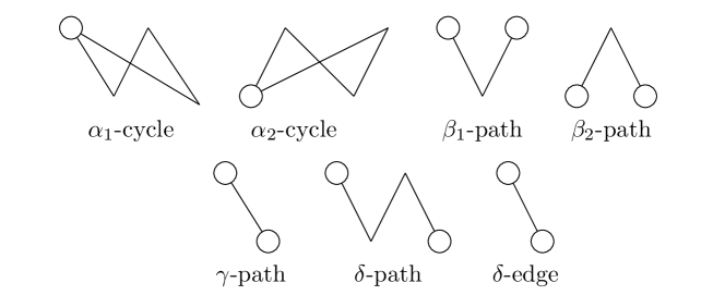
In the graph $G^{\prime}$, a path whose end vertices are distinct special points is said to be a special path and a cycle which contains exactly one special point is said to be a special cycle. Since $G^{\prime}$ is connected and $\mathrm{deg}(v)\geq 2$, it is clear that it consists of such special paths and cycles which are disjoint except at special points. We classify these special paths and cycles into seven types and contract them to the minimal ones as in Figure 3 to obtain the basic graph $\mathcal{B}(G)$.

• An $\alpha_{i}$-cycle is a special cycle with exactly one special point in $V_{i}^{\prime}$ ($i=1,2$). By the structure of bipartite graphs, these special cycles contain at least three normal points. The minimal $\alpha_{i}$-cycle has three normal points as in Figure 3.

• A $\beta_{j}$-path is a special path whose end vertices are two distinct special points in $V_{j}^{\prime}$ ($j=1,2$). By the structure of bipartite graphs, these special paths contain at least one normal point. The minimal $\beta_{j}$-path has only one normal point as in Figure 3.

• A special path whose end vertices are special points in $V_{1}^{\prime}$ and $V_{2}^{\prime}$ is called in several ways according to the situation. For each pair of special points $v_{1}\in V_{1}^{\prime}$ and $v_{2}\in V_{2}^{\prime}$, we have two cases.

  • Case(i) there is only one special path connecting $v_{1}$ and $v_{2}$: such a special path is called a $\gamma$-path. The length of the minimal $\gamma$-path is one.

  • Case(ii) there is more than one special path connecting $v_{1}$ and $v_{2}$: since we are considering a simple graph, there is at most one such a special path of length one, i.e., joined by an edge. A special path is called a $\delta$-path if the length is three or more and a $\delta$-edge if the length is one. The length of the minimal $\delta$-path is three.

We decomposed $G^{\prime}$ into the union of a collection of $\alpha_{i}$-cycles, $\beta_{j}$-paths, $\gamma$-paths, $\delta$-paths, and $\delta$-edges. The basic graph $\mathcal{B}(G)$ is obtained from $G^{\prime}$ by contracting $\alpha_{i}$-cycles, $\beta_{j}$-paths, $\gamma$-paths, and $\delta$-paths to the minimal ones as in Figure 3. In the procedure of contraction, we forget about labels of vertices. We summarize the contraction procedures below.

• If each $\alpha_{i}$-cycle ($i=1,2$) contains five or more normal points, we contract it to the minimal $\alpha_{i}$-cycle, which has three normal points.

• If each $\beta_{j}$-path ($j=1,2$) contains three or more normal points, we contract it to the minimal $\beta_{j}$-path, which has only one normal point.

• If each $\gamma$-path contains normal points, we contract it to the minimal $\gamma$-path, which has no normal points.

• If each $\delta$-path contains four or more normal points, we contract it to the minimal $\delta$-path, which has two normal points.

Figure 3. Seven types of minimal special paths, cycles and edge. The circles denote special points.

We have seen how to make the basic graph $\mathcal{B}(G)$ from a given labeled connected bipartite $(r,s,r+s-1+k)$-graph $G$. Note that the number of cycles in graphs is invariant by the contractions, so that $\mathcal{B}(G)$ has just $k$ cycles. We will reconstruct labeled bipartite graphs from each basic graph $\mathcal{B}$ and introduce $J_{\mathcal{B}}(x,y)$ to express $F_{k}(x,y)$ as sum of $J_{\mathcal{B}}(x,y)$’s.

Proof of Theorem 1.6.

For a given labeled connected bipartite $(r,s,r+s-1+k)$-graph $G$, let $V^{\prime\prime}=(V_{1}^{\prime\prime},V_{2}^{\prime\prime})$ be the vertex set of $\mathcal{B}(G)$, and also let $a_{i},b_{j},c,d$ and $e$ be the number of $\alpha_{i}$-cycles, $\beta_{j}$-paths, $\gamma$-paths, $\delta$-paths, and $\delta$-edges in $\mathcal{B}(G)$, respectively. Then, for the number of vertices in $\mathcal{B}(G)$, we have

$$|V_{1}^{\prime\prime}| =r_{\rm sp}+a_{1}+2a_{2}+b_{2}+d\leq t\leq r,$$ (5.2)

$$|V_{2}^{\prime\prime}| =s_{\rm sp}+2a_{1}+a_{2}+b_{1}+d\leq u\leq s.$$ (5.3)

For the number of edges in $\mathcal{B}(G)$, since the same number of vertices and edges are deleted by contraction, we have

$$4a_{1}+4a_{2}+2b_{1}+2b_{2}+c+3d+e=|V_{1}^{\prime\prime}|+|V_{2}^{\prime\prime}|+k-1.$$ (5.4)

Combining (5.2)-(5.4) and the inequality (5.1), we have

$$a_{1}+a_{2}+b_{1}+b_{2}+c+d+e =r_{\rm sp}+s_{\rm sp}+k-1$$

$$\leq 3(k-1).$$ (5.5)

Therefore, if $G$ is a labeled connected bipartite $(r,s,r+s-1+k)$-graph, then $\mathcal{B}(G)$ should satisfy the conditions (5.1)-(5.1). Now we denote the set of all possible basic graphs having $k$ cycles by $BG_{k}$, i.e.,

$$BG_{k}:=\{\mathcal{B}(G):\text{$G$ is a labeled bipartite $(r,s,r+s-1+k)$-graph for some $r,s$}.\}$$

It follows from (5.1) that $BG_{k}$ is a finite set.

For fixed $\mathcal{B}\in BG_{k}$, let $j_{\mathcal{B}}(r,s)$ be the number of labeled connected bipartite $(r,s,r+s-1+k)$-graphs $G$ such that $\mathcal{B}(G)=\mathcal{B}$. We define the exponential generating function of $j_{\mathcal{B}}(r,s)$ as

$$J_{\mathcal{B}}=J_{\mathcal{B}}(x,y):=\sum_{r,s=0}^{\infty}j_{\mathcal{B}}(r,s)\frac{x^{r}y^{s}}{r!s!}.$$

We will show below that $J_{\mathcal{B}}(x,y)$ is expressed by a rational function of $T_{x}$ and $T_{y}$. To this end, we count $j_{\mathcal{B}}(r,s)$ by reversing the procedure of contraction above, i.e., by adding pairs of a normal point and its adjacent edge in $\mathcal{B}$ and rearranging labels of $(r,s)$ vertices. We construct bipartite $(r,s,r+s-1+k)$-graphs from $\mathcal{B}$ by two steps as follows.
Step 1: Take $\mathcal{B}\in BG_{k}$. Let $V^{\prime\prime}=(V_{1}^{\prime\prime},V_{2}^{\prime\prime})$ be the vertex set of $\mathcal{B}$ and $M:=a_{1}+a_{2}+b_{1}+b_{2}+c+d$ be the number of all minimal special paths and cycles in $\mathcal{B}$ except $\delta$-edges. Take $t$ and $u$ such that $|V_{1}^{\prime\prime}|\leq t\leq r$ and $|V_{2}^{\prime\prime}|\leq u\leq s$. We label all minimal $\alpha_{i}$-cycles, $\beta_{j}$-paths, $\gamma$-paths and $\delta$-paths in $\mathcal{B}$, say, $\mathsf{s}_{1},\mathsf{s}_{2},\dots,\mathsf{s}_{M}$, and we add pairs of a normal point and its adjacent edge in these special paths/cycles. By the structure of bipartite graphs, for every $j=1,2,\dots,M$, the number of added pairs in each $\mathsf{s}_{j}$ is even, and the numbers of added normal points in $V_{1}^{\prime\prime}$ and $V_{2}^{\prime\prime}$ are equal, which we denote by $m_{j}$. Hence, a necessary condition for the numbers of added vertices in $V_{1}^{\prime\prime}$ and $V_{2}^{\prime\prime}$ is $t-|V_{1}^{\prime\prime}|=u-|V_{2}^{\prime\prime}|=\sum_{j=1}^{M}m_{j}$. Combining (5.2) and (5.3) with the necessary condition, the non-negative integers $\{m_{j}\}_{j=1}^{M}$ satisfy

$$m_{1}+m_{2}+\cdots+m_{M} =t-(r_{\rm sp}+a_{1}+2a_{2}+b_{2}+d),$$ (5.6)

$$m_{1}+m_{2}+\cdots+m_{M} =u-(s_{\rm sp}+2a_{1}+a_{2}+b_{1}+d).$$ (5.7)

Let $y_{\mathcal{B}}(t,u)=y_{\mathcal{B}}(t,u,r_{{\rm sp}},s_{{\rm sp}},a_{1},a_{2},b_{1},b_{2},c,d)$ be the number of the solutions $\{m_{j}\}_{j=1}^{M}$ of (5.6) and (5.7). For each solution $\{m_{j}\}_{j=1}^{M}$, we obtain an unlabeled connected bipartite $(t,u,t+u-1+k)$-graph, and hence $y_{\mathcal{B}}(t,u)$ of those from $\mathcal{B}$.
Step 2: Take one of $y_{\mathcal{B}}(t,u)$ of unlabeled connected bipartite $(t,u,t+u-1+k)$-graphs and call its vertices $T_{1},\dots,T_{t}$ and $U_{1},\dots,U_{u}$. Let $\mathcal{I}_{t,u}$ the set of $\{(r_{1i},s_{1i})\}_{i=1}^{t}$ and $\{(r_{2j},s_{2j})\}_{j=1}^{u}$ such that $r_{1i}\geq 1,r_{2j}\geq 0,s_{1i}\geq 0,s_{2j}\geq 1$, $\sum\limits_{i=1}^{t}r_{1i}+\sum\limits_{j=1}^{u}r_{2j}=r$ and $\sum\limits_{i=1}^{t}s_{1i}+\sum\limits_{j=1}^{u}s_{2j}=s$. For each $\{(r_{1i},s_{1i})\}_{i=1}^{t}$ and $\{(r_{2j},s_{2j})\}_{j=1}^{u}$ in $\mathcal{I}_{t,u}$, we attach a rooted tree of size $(r_{1i},s_{1i})$ to $T_{i}$ for $i=1,2,\dots,t$ and a rooted tree of size $(r_{2j},s_{2j})$ to $U_{j}$ for $j=1,2,\dots,u$, respectively. Let $N(r,s,t,u)$ be the number of these bipartite $(r,s,r+s-1+k)$-graphs. Then, by counting $t$ rooted trees whose roots are in $V_{1}$ and $u$ rooted trees whose roots are in $V_{2}$, we have

$$N(r,s,t,u) =\sum\nolimits^{\prime}\binom{r}{r_{11},\dots,r_{1t},r_{21},\dots,r_{2u}}\binom{s}{s_{11},\dots,s_{1t},s_{21},\dots,s_{2u}}$$

$$\quad\times\prod_{i=1}^{t}r_{1i}^{s_{1i}}s_{1i}^{r_{1i}-1}\prod_{j=1}^{u}r_{2j}^{s_{2j}-1}s_{2j}^{r_{2j}},$$ (5.8)

where the summation $\sum\nolimits^{\prime}$ is taken over the set $\mathcal{I}_{t,u}$.
By the above two steps, we obtain all labeled connected bipartite $(r,s,r+s-1+k)$-graphs from the basic graph $\mathcal{B}$. However, not all of them are different because of forgetting labels $\mathsf{s}_{1},\dots,\mathsf{s}_{M}$ after attaching labeled rooted trees to all vertices. Indeed, if $g_{\mathcal{B}}$ is the number of automorphisms of $\mathcal{B}$, then every graph appears exactly $g_{\mathcal{B}}$ times. Hence, we have

$$j_{\mathcal{B}}(r,s)=\sum_{\begin{subarray}{c}|V_{1}^{\prime\prime}|\leq t\leq r\\ |V_{2}^{\prime\prime}|\leq u\leq s\end{subarray}}\frac{y_{\mathcal{B}}(t,u)N(r,s,t,u)}{g_{\mathcal{B}}}.$$

Using this, we have

$$J_{\mathcal{B}}(x,y)=\frac{1}{g_{\mathcal{B}}}\sum_{\begin{subarray}{c}|V_{1}^{\prime\prime}|\leq t\\ |V_{2}^{\prime\prime}|\leq u\end{subarray}}y_{\mathcal{B}}(t,u)\sum_{\begin{subarray}{c}t\leq r\\ u\leq s\end{subarray}}N(r,s,t,u)\frac{x^{r}y^{s}}{r!s!}.$$ (5.9)

For the summation in $r$ and $s$, by (5.1), we have

$$\sum_{\begin{subarray}{c}t\leq r\\ u\leq s\end{subarray}}N(r,s,t,u)\frac{x^{r}y^{s}}{r!s!} =\sum_{\begin{subarray}{c}t\leq r\\ u\leq s\end{subarray}}\sum\nolimits^{\prime}\prod_{i=1}^{t}r_{1i}^{s_{1i}}s_{1i}^{r_{1i}-1}\frac{x^{r_{1i}}y^{s_{1i}}}{r_{1i}!s_{1i}!}\prod_{j=1}^{u}r_{2j}^{s_{2j}-1}s_{2j}^{r_{2j}}\frac{x^{r_{2j}}y^{s_{2j}}}{r_{2j}!s_{2j}!}$$

$$=T_{x}^{t}T_{y}^{u}.$$

On the other hand, by a straightforward calculation, we have

$$\sum_{\begin{subarray}{c}|V_{1}^{\prime\prime}|\leq t\\ |V_{2}^{\prime\prime}|\leq u\end{subarray}}y_{\mathcal{B}}(t,u)T_{x}^{t}T_{y}^{u} =\sum_{\begin{subarray}{c}|V_{1}^{\prime\prime}|\leq t\\ |V_{2}^{\prime\prime}|\leq u\end{subarray}}\ \sum_{\begin{subarray}{c}m_{1},\dots,m_{M}\\ \sum m_{j}=t-|V_{1}^{\prime\prime}|=u-|V_{2}^{\prime\prime}|\end{subarray}}T_{x}^{t}T_{y}^{u}$$

$$=T_{x}^{|V_{1}^{\prime\prime}|}T_{y}^{|V_{2}^{\prime\prime}|}\sum_{\begin{subarray}{c}|V_{1}^{\prime\prime}|\leq t\\ |V_{2}^{\prime\prime}|\leq u\end{subarray}}\ \sum_{\begin{subarray}{c}m_{1},\dots,m_{M}\\ \sum m_{j}=t-|V_{1}^{\prime\prime}|=u-|V_{2}^{\prime\prime}|\end{subarray}}(T_{x}T_{y})^{\sum_{j=1}^{M}m_{j}}$$

$$=T_{x}^{|V_{1}^{\prime\prime}|}T_{y}^{|V_{2}^{\prime\prime}|}\sum_{n\geq 0}\ \sum_{\begin{subarray}{c}m_{1},\dots,m_{M}\\ \sum m_{j}=n\end{subarray}}(T_{x}T_{y})^{\sum_{j=1}^{M}m_{j}}$$

$$=T_{x}^{|V_{1}^{\prime\prime}|}T_{y}^{|V_{2}^{\prime\prime}|}\prod_{j=1}^{M}\Bigl{(}\sum_{m_{j}\geq 0}(T_{x}T_{y})^{m_{j}}\Bigr{)}$$

$$=T_{x}^{|V_{1}^{\prime\prime}|}T_{y}^{|V_{2}^{\prime\prime}|}(1-T_{x}T_{y})^{-M}.$$ (5.10)

Combining (5.2), (5.3), (5.1), (5.9) and (5.1), we obtain (1.12). Since non-isomorphic basic graphs with $k$ cycles lead non-isomorphic labeled connected bipartite $(r,s,r+s-1+k)$-graphs, taking a summation $J_{\mathcal{B}}$ with respect to $\mathcal{B}\in BG_{k}$, we obtain (1.11), which completes the proof. ∎

We give an example of Theorem 1.6 for $k=2$.

Example 5.1 ($k=2$).

Let us consider all the basic graphs for $k=2$ and compute $F_{2}(x,y)$. From the conditions (5.1) and (5.1), we have

$$r_{\mathrm{sp}}+s_{\mathrm{sp}}\leq 2,$$

$$a_{1}+a_{2}+b_{1}+b_{2}+c+d+e=r_{\mathrm{sp}}+s_{\mathrm{sp}}+1.$$

As a result, the possible combinations of numbers of special points are $(r_{\mathrm{sp}},s_{\mathrm{sp}})=(1,0),(0,1),(1,1),(2,0),(0,2)$. We compute $J_{\mathcal{B}}$ for each of these cases. For instance, the calculation procedure is described below for the case of $(r_{\mathrm{sp}},s_{\mathrm{sp}})=(1,0)$. First, consider the numbers of cycles, paths and edges that make up the basic graphs. The following should be obvious. By using

$$a_{1}+a_{2}+b_{1}+b_{2}+c+d+e=2,$$

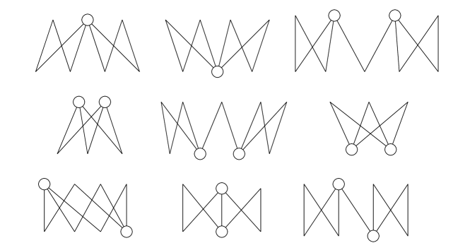
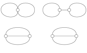
we have $(a_{1},a_{2},b_{1},b_{2},c,d,e)=(2,0,0,0,0,0,0)$. As a result, the basic graph is a combination of two $\alpha_{1}$-cycles. This is the upper left graph in Figure 4. We define this basic graph as $\mathcal{B}_{1}$. Note that basic graphs are unlabeled.

Next, let us compute the number of graph automorphism $g_{\mathcal{B}_{1}}$. We label each of the vertices appropriately. For the labeled basic graph, there are $2!$ ways to arrange the two $\alpha_{1}$-cycles. There are two possible ways to label the vertices of each $\alpha_{1}$-cycle: $1\to 2\to 3\to 4\to 1$ with the special point as 1, or in reverse $1\to 4\to 3\to 2\to 1$. Therefore $g_{\mathcal{B}_{1}}=2!\times 2^{2}=8$. Consequently, from (1.12) we obtain

$$J_{\mathcal{B}_{1}}(x,y)=\frac{T_{x}^{3}T_{y}^{4}}{8(1-T_{x}T_{y})^{2}}.$$

We can derive the others by the same calculation. Therefore,

$$\sum_{\mathcal{B}\in BG_{2}}J_{\mathcal{B}}(x,y)= \frac{T_{x}^{3}T_{y}^{4}}{8(1-T_{x}T_{y})^{2}}+\frac{T_{x}^{4}T_{y}^{3}}{8(1-T_{x}T_{y})^{2}}+\frac{T_{x}^{4}T_{y}^{5}}{8(1-T_{x}T_{y})^{3}}$$

$$+\frac{T_{x}^{2}T_{y}^{3}}{12(1-T_{x}T_{y})^{3}}+\frac{T_{x}^{5}T_{y}^{4}}{8(1-T_{x}T_{y})^{3}}+\frac{T_{x}^{3}T_{y}^{2}}{12(1-T_{x}T_{y})^{3}}$$

$$+\frac{T_{x}^{4}T_{y}^{4}}{6(1-T_{x}T_{y})^{3}}+\frac{T_{x}^{3}T_{y}^{3}}{2(1-T_{x}T_{y})^{2}}+\frac{T_{x}^{4}T_{y}^{4}}{4(1-T_{x}T_{y})^{3}}$$

$$= \frac{W^{2}(2+3W)}{24(1-W)^{3}}Z+\frac{W^{3}(6-W)}{12(1-W)^{3}}$$

$$= F_{2}(x,y),$$

where the nine terms correspond to the nine basic graphs in Figure 4, respectively. Hence, the result of the calculation by using basic graphs is consistent with $F_{2}(x,y)=f_{2}(Z,W)$.

Figure 4. Basic graphs for $k=2$

5.2. Proof of Theorem 1.7

From (1.11), (1.12) and (5.1), we see that

$$F_{k}(x,y)=\frac{1}{(1-T_{x}T_{y})^{3(k-1)}}\sum_{\mathcal{B}\in BG_{k}}\frac{1}{g_{\mathcal{B}}}T_{x}^{r_{\mathcal{B}}}T_{y}^{s_{\mathcal{B}}}(1-T_{x}T_{y})^{p_{\mathcal{B}}},$$ (5.11)

where $r_{\mathcal{B}}=r_{{\rm sp}}+a_{1}+2a_{2}+b_{2}+d$, $s_{\mathcal{B}}=s_{{\rm sp}}+2a_{1}+a_{2}+b_{1}+d$, and

$$p_{\mathcal{B}} =3(k-1)-(a_{1}+a_{2}+b_{1}+b_{2}+c+d)$$

$$=2(k-1)-(r_{{\rm sp}}+s_{{\rm sp}})+e$$

$$=\sum_{v\in\text{special points}}(\mathrm{deg}(v)-3)+e$$

$$\geq 0.$$ (5.12)

Note that there are some basic graphs $\mathcal{B}\in BG_{k}$ such that $p_{\mathcal{B}}=0$. For example, we can construct a basic graph $\tilde{\mathcal{B}}$ with $r_{{\rm sp}}=2(k-1)$, $a_{1}=2$, $b_{1}=3k-5$ and other constants vanishing as follows: we label all $2(k-1)$ special points in $V_{1}$, say, $r_{1},r_{2},\dots,r_{2(k-1)}$. We attach an $\alpha_{1}$-cycle to each of $r_{1}$ and $r_{2(k-1)}$, and then connect $r_{2j-1}$ with $r_{2j}$ ($j=1,2,\dots,k-1$) by a $\beta_{1}$-path and $r_{2j}$ with $r_{2j+1}$ ($j=1,2,\dots,k-2$) by two $\beta_{1}$-paths. Then, we obtain $\tilde{\mathcal{B}}$. Remark that in the case of $k=2$, $\tilde{\mathcal{B}}$ corresponds to the top-right graph in Figure 4. Clearly, $s_{{\rm sp}}=e=0$ holds for all $k\geq 2$, and the calculation in (5.12) gives $p_{\tilde{\mathcal{B}}}=0$. From this observation, the numerator of the right-hand side of (5.11) turns out to be a polynomial of the following form

$$Q(x,y)=\sum_{i=1}^{m}C_{i}x^{a_{i}}y^{b_{i}}+\sum_{i=m+1}^{m+n}C_{i}x^{a_{i}}y^{b_{i}}(1-xy)^{p_{i}},$$

for some positive integers $m$ and $n$. Here $a_{i},b_{i}$ are non-negative integers, $p_{i}$ is a positive integer and $C_{i}>0$ for all $i$. If $Q(x,y)$ has a factor $1-xy$, plugging $y=x^{-1}$ in both sides yields $0=\sum_{i=1}^{m}C_{i}>0$, which is a contradiction. Hence, $Q(x,y)$ does not have the factor $1-xy$, which implies that the numerator of the right-hand side of (5.11) does not have a factor $1-T_{x}T_{y}$.

We will prove (1.13). Assume $\mathcal{B}=(V,E)$ with bipartition $V=V_{1}\sqcup V_{2}$. We have the following lemma.

Lemma 5.2.

For any $\mathcal{B}\in BG_{k}$, $\big{|}|V_{1}|-|V_{2}|\big{|}\leq k-1$.

Proof.

Since $\mathrm{deg}(v)\geq 2$ for every vertex $v$ in a basic graph $\mathcal{B}$, we see that

$$|E|-|V|-\big{|}|V_{1}|-|V_{2}|\big{|}=|E|-2\max(|V_{1}|,|V_{2}|)\geq 0.$$

On the other hand, $|E|-|V|=k-1$ since $\mathcal{B}$ is connected and $k$ is the Betti number. Therefore, $\big{|}|V_{1}|-|V_{2}|\big{|}\leq k-1$. ∎

For $\mathcal{B}=(V_{1}\sqcup V_{2},E)\in BG_{k}$, there exists a unique basic graph $\mathcal{B}^{\prime}=(V_{1}^{\prime}\sqcup V_{2}^{\prime},E^{\prime})\in BG_{k}$ such that $V_{1}^{\prime}=V_{2},V_{2}^{\prime}=V_{1}$, and $E^{\prime}=E$. Let $\pi:BG_{k}\to BG_{k}$ be a mapping defined by $\pi(\mathcal{B})=\mathcal{B}^{\prime}$. Then $\pi$ is an involution, and we have

$$g_{\pi(\mathcal{B})}=g_{\mathcal{B}},\quad r_{\pi(\mathcal{B})}=s_{\mathcal{B}},\quad s_{\pi(\mathcal{B})}=r_{\mathcal{B}},\quad p_{\pi(\mathcal{B})}=p_{\mathcal{B}},$$ (5.13)

where $r_{\mathcal{B}}=|V_{1}|$, $s_{\mathcal{B}}=|V_{2}|$. From this involution with (5.13), the numerator of (5.11) turns out to be

$$\sum_{\mathcal{B}\in BG_{k}}\frac{1}{g_{\mathcal{B}}}T_{x}^{r_{\mathcal{B}}}T_{y}^{s_{\mathcal{B}}}(1-T_{x}T_{y})^{p_{\mathcal{B}}}$$

$$=\sum_{\begin{subarray}{c}\mathcal{B}\in BG_{k}\\ r_{\mathcal{B}}>s_{\mathcal{B}}\end{subarray}}\frac{(T_{x}T_{y})^{s_{\mathcal{B}}}}{g_{\mathcal{B}}}(T_{x}^{q_{\mathcal{B}}}+T_{y}^{q_{\mathcal{B}}})(1-T_{x}T_{y})^{p_{\mathcal{B}}}+\sum_{\begin{subarray}{c}\mathcal{B}\in BG_{k}\\ r_{\mathcal{B}}=s_{\mathcal{B}}\end{subarray}}\frac{(T_{x}T_{y})^{r_{\mathcal{B}}}}{g_{\mathcal{B}}}(1-T_{x}T_{y})^{p_{\mathcal{B}}},$$ (5.14)

where $q_{\mathcal{B}}=r_{\mathcal{B}}-s_{\mathcal{B}}$. Since $T_{x}^{q_{\mathcal{B}}}+T_{y}^{q_{\mathcal{B}}}$ is a polynomial of $Z$ of degree $q_{\mathcal{B}}$ with coefficients being polynomials of $W$, so is the right-hand side of (5.14) but the degree is equal to $\max_{\mathcal{B}\in BG_{k},r_{\mathcal{B}}>s_{\mathcal{B}}}q_{\mathcal{B}}$. Now we consider a basic graph $\hat{\mathcal{B}}$ which has one special point in $V_{2}$ and $k$ $\alpha_{2}$-cycles. Clearly, $r_{\hat{\mathcal{B}}}=2k,s_{\hat{\mathcal{B}}}=k+1$ hold, and hence $q_{\hat{\mathcal{B}}}=k-1$. This together with Lemma 5.2 implies $\max_{\mathcal{B}\in BG_{k},r_{\mathcal{B}}>s_{\mathcal{B}}}q_{\mathcal{B}}=k-1$. Since $\mathcal{B}$ is a simple graph and has at least one cycle, we have $r_{\mathcal{B}},s_{\mathcal{B}}\geq 2$. Then, the right hand side of (5.14) has a factor $(T_{x}T_{y})^{2}=W^{2}$. Thus the proof of (1.13) is completed.

5.3. Combinatorial proof of Proposition 1.1

Finally, we remark on another proof of Proposition 1.1 using a similar argument in the proof of Theorem 1.6, which is a bipartite version of the combinatorial argument discussed in [12, Section 5]. We use the same notation as above. In the preliminary step, we delete leaves and adjacent edges repeatedly. In this case, by this procedure, we obtain the unique cycle of length, say $2t$. Let $r,s\geq 2$ be fixed and $V^{\prime\prime}=(V_{1}^{\prime\prime},V_{2}^{\prime\prime})$ be a vertex set. Take $t$ such that $2\leq t\leq\min\{r,s\}$, and consider an unlabeled bipartite unicyclic graph whose length of the cycle is $2t$. Clearly, $|V_{1}^{\prime\prime}|=|V_{2}^{\prime\prime}|=t$. For each of vertices of this graph, we attach a rooted tree in a similar way of Step 2 in the proof of Theorem 1.6. To create $2t$ rooted trees, we partition $(r,s)$ vertices into $2t$ vertex sets, and all of these partitions are in $\mathcal{I}_{t,t}$. By this procedure, we obtain $N(r,s,t,t)$ labeled connected bipartite $(r,s,r+s)$-graphs, where $N(r,s,t,u)$ is defined in (5.1). For each of the obtained graphs, there are $2t$ automorphisms due to the cycle and labels of roots of rooted trees. Let $j(r,s)$ be the number of labeled connected bipartite $(r,s,r+s)$-graphs. Then, we have

$$j(r,s)=\sum_{2\leq t\leq\min\{r,s\}}\frac{N(r,s,t,t)}{2t}.$$

Let $J(x,y)$ be the exponential generating function for $j(r,s)$, and we have

$$J(x,y) =\sum_{r,s=0}^{\infty}j(r,s)\frac{x^{r}y^{s}}{r!s!}=\sum_{t=2}^{\infty}\frac{1}{2t}\sum_{\begin{subarray}{c}t\leq r\\ t\leq s\end{subarray}}\frac{N(r,s,t,t)}{r!s!}x^{r}y^{s}$$

$$=\frac{1}{2}\sum_{t=2}^{\infty}\frac{(T_{x}T_{y})^{t}}{t}=-\frac{1}{2}(\log(1-T_{x}T_{y})+T_{x}T_{y})=F_{1}(x,y),$$

which completes the combinatorial proof of Proposition 1.1.

6. Proof of Theorem 1.5

In this section, we prove the asymptotic equality (1.10) for $k\geq 2$. In Subsection 6.1, for each basic graph $\mathcal{B}\in BG_{k}$, we find the leading term of $J_{\mathcal{B}}(x,x)$ by a combinatorial argument, where the multigraph $\mathcal{B}^{*}$ obtained from $\mathcal{B}$ by contraction plays an important role. In Subsection 6.2, we introduce the basic graphs on complete graphs as discussed in [12] and give a similar discussion in Subsection 6.1, and in Subsection 6.3, we derive the leading asymptotic behavior of $N_{\rm{bi}}(n,k)$ defined by (1.8). Through the existence of multigraphs, we will see the correspondence between basic graphs on complete bipartite graphs and those on complete graphs.

6.1. Basic graphs $\mathcal{B}$ and $J_{\mathcal{B}}(x,x)$

Let us recall again $Y(x)$ in (4.14) representing exponential generating function for labeled rooted trees. From (LABEL:eq:diagonalZW), $Z(x,x)=2Y(x)$ and $W(x,x)=Y(x)^{2}$. Recall that

$$Z(x,y)=T_{x}(x,y)+T_{y}(x,y),\ \ W(x,y)=T_{x}(x,y)T_{y}(x,y).$$

Solving these equations, we have

$$T_{x}(x,x)=T_{y}(x,x)=Y(x).$$ (6.1)

From Theorem 1.6, for $k\geq 2$ we have

$$F_{k}(x,x)=\sum_{\mathcal{B}\in BG_{k}}J_{\mathcal{B}}(x,x),$$

where

$$J_{\mathcal{B}}(x,x)=\dfrac{Y^{L}}{g_{\mathcal{B}}(1-Y^{2})^{M}},$$ (6.2)

with $M=M(\mathcal{B}):=a_{1}+a_{2}+b_{1}+b_{2}+c+d$ and $L=L(\mathcal{B}):=M+r_{{\rm sp}}+s_{{\rm sp}}+2a_{1}+2a_{2}-c+d$. These constants are determined by $\mathcal{B}$. In this section, we also use the notation $a_{1}=a_{1}(\mathcal{B}),r_{{\rm sp}}=r_{{\rm sp}}(\mathcal{B})$, and so on. We easily see the following.

Lemma 6.1.

For $\mathcal{B}\in BG_{k}$, there exist unique constants $\{\mathfrak{a}_{i}(\mathcal{B})\}_{i=1}^{M},\{\mathfrak{b}_{i}(\mathcal{B})\}_{i=1}^{M},\{\mathfrak{c}_{j}(\mathcal{B})\}_{j=0}^{L-2M}$ such that

$$J_{\mathcal{B}}(x,x)=\sum_{i=1}^{M}\left(\frac{\mathfrak{a}_{i}(\mathcal{B})}{(1-Y)^{i}}+\frac{\mathfrak{b}_{i}(\mathcal{B})}{(1+Y)^{i}}\right)+\sum_{j=0}^{L-2M}\mathfrak{c}_{j}(\mathcal{B})Y^{j}.$$ (6.3)

In particular,

$$\mathfrak{a}_{M}(\mathcal{B})=\frac{1}{g_{\mathcal{B}}2^{M}},\ \ \mathfrak{b}_{M}(\mathcal{B})=\frac{(-1)^{L}}{g_{\mathcal{B}}2^{M}}.$$ (6.4)

Proof.

Multiplying both sides of (6.2) and (6.3) by $(1-Y^{2})^{M}$ and substituting $Y=\pm 1$ yield (6.4). ∎

For each $\mathcal{B}\in BG_{k}$, we contract its special cycles and paths and ignore the vertex set $V=(V_{1},V_{2})$. By this procedure, we obtain a multigraph $\mathcal{B}^{*}$ from $\mathcal{B}$. Let $MG_{k}$ be the set of all multigraphs obtained from $BG_{k}$ by this procedure. Define a mapping $\phi:BG_{k}\to MG_{k}$ by $\phi(\mathcal{B})=\mathcal{B}^{*}$ and for $\mathcal{B}^{*}\in MG_{k}$,

$$\phi^{-1}(\mathcal{B}^{*}):=\{\mathcal{B}\in BG_{k}:\phi(\mathcal{B})=\mathcal{B}^{*}\}.$$

All basic graphs which belong to $\phi^{-1}(\mathcal{B}^{*})$ have the same number of special cycles and the same total number of special paths and edges. In what follows in this section, we only consider basic graphs $\mathcal{B}\in BG_{k}$ such that $M(\mathcal{B})=3(k-1)$ and multigraphs $\mathcal{B}^{*}\in MG_{k}$ obtained from such basic graphs $\mathcal{B}$. From (5.1), it follows that such a $\mathcal{B}$ has no $\delta$-edge, i.e., $e(\mathcal{B})=0$ and $r_{{\rm sp}}(\mathcal{B})+s_{{\rm sp}}(\mathcal{B})=2(k-1)$ holds. For given $\mathcal{B}^{*}\in MG_{k}$, we divide the set $\phi^{-1}(\mathcal{B}^{*})$ by pairs of $(r_{{\rm sp}}(\mathcal{B}),s_{{\rm sp}}(\mathcal{B}))$. For $i=0,\dots,2(k-1)$, define

$$\phi^{-1}(\mathcal{B}^{*})^{(2(k-1)-i,i)}:=\{\mathcal{B}\in\phi^{-1}(\mathcal{B}^{*}):(r_{{\rm sp}}(\mathcal{B}),s_{{\rm sp}}(\mathcal{B}))=(2(k-1)-i,i)\}.$$

Then, we have

$$\phi^{-1}(\mathcal{B}^{*})=\bigsqcup_{0\leq i\leq 2(k-1)}\phi^{-1}(\mathcal{B}^{*})^{(2(k-1)-i,i)}.$$ (6.5)

Note that $\phi^{-1}(\mathcal{B}^{*})^{(2(k-1),0)}$ and $\phi^{-1}(\mathcal{B}^{*})^{(0,2(k-1))}$ are singletons, and each of the element is determined by $\mathcal{B}^{*}$ in a clear way. Indeed, if $\mathcal{B}^{*}$ has self-loops, replace them to minimal $\alpha_{1}$-cycles. Also, if $\mathcal{B}^{*}$ has single edges or multiple edges, replace them to $\beta_{1}$-paths. Putting all vertices of $\mathcal{B}^{*}$ in $V_{1}$ and by this procedure, we obtain a basic graph $\mathcal{B}\in\phi^{-1}(\mathcal{B}^{*})^{(2(k-1),0)}$. Clearly, the obtained graph $\mathcal{B}$ is unique. In a similar way, we have a unique element in $\phi^{-1}(\mathcal{B}^{*})^{(0,2(k-1))}$. For the following discussion, we denote by $\mathcal{B}_{{\rm id}}$ the unique element in $\phi^{-1}(\mathcal{B}^{*})^{(2(k-1),0)}$.

Lemma 6.2.

Let $\mathcal{B}^{*}\in MG_{k}$ be given. Then, for $i=0,\dots,2(k-1)$,

$$\sum_{\begin{subarray}{c}\mathcal{B}\in\phi^{-1}(\mathcal{B}^{*})^{(2(k-1)-i,i)}\\ M(\mathcal{B})=3(k-1)\end{subarray}}\frac{1}{g_{\mathcal{B}}}=\binom{2(k-1)}{i}\frac{1}{g_{\mathcal{B}_{{\rm id}}}}.$$ (6.6)

Proof.

For $i=0$, $\mathcal{B}_{{\rm id}}$ and $g_{\mathcal{B}_{{\rm id}}}$ are determined by $\mathcal{B}^{*}$. Clearly, $r_{{\rm sp}}(\mathcal{B}_{{\rm id}})=2(k-1)$ holds. We label all $2(k-1)$ special points of $\mathcal{B}_{{\rm id}}$, and we construct $\mathcal{B}\in\phi^{-1}(\mathcal{B}^{*})^{(2(k-1)-i,i)},i=0,\dots,2(k-1)$ by the following way. For given $i$, we choose $\binom{2(k-1)}{i}$ labeled special points in $\mathcal{B}_{{\rm id}}$, and we put these points in $V_{2}$ without changing the connectivity of the vertices. Here, for each $\beta_{1}$-path in $\mathcal{B}_{{\rm id}}$, delete or add a normal point to create $\gamma$-path or $\delta$-path from it. Then, we have $\binom{2(k-1)}{i}$ basic graphs $\mathcal{B}_{1},\cdots,\mathcal{B}_{\binom{2(k-1)}{i}}$ from $\mathcal{B}_{{\rm id}}$ which satisfy $(r_{{\rm sp}},s_{{\rm sp}})=(2(k-1)-i,i)$. Since this procedure does not change the connectivity of graphs, the numbers of the automorphisms of obtained graphs $\{\mathcal{B}_{\ell}\}_{\ell=1}^{\binom{2(k-1)}{i}}$ are $g_{\mathcal{B}_{{\rm id}}}$. To obtain $\phi^{-1}(\mathcal{B}^{*})^{(2(k-1)-i,i)}$, we forget all labels of special points of $\{\mathcal{B}_{\ell}\}_{\ell=1}^{\binom{2(k-1)}{i}}$. Nevertheless each of ${\binom{2(k-1)}{i}}$ unlabeled graphs may not be different, we have

$$\sum_{\begin{subarray}{c}\mathcal{B}\in\phi^{-1}(\mathcal{B}^{*})^{(2(k-1)-i,i)}\\ M(\mathcal{B})=3(k-1)\end{subarray}}\frac{1}{g_{\mathcal{B}}}=\sum_{\ell=0}^{{\binom{2(k-1)}{i}}}\frac{1}{g_{\mathcal{B}_{\ell}}}=\binom{2(k-1)}{i}\frac{1}{g_{\mathcal{B}_{{\rm id}}}}.$$

∎

Proposition 6.3.

For $\mathcal{B}^{*}\in MG_{k}$,

$$\sum_{\begin{subarray}{c}\mathcal{B}\in\phi^{-1}(\mathcal{B}^{*})\\ M(\mathcal{B})=3(k-1)\end{subarray}}\mathfrak{b}_{3(k-1)}(\mathcal{B})=0.$$

To show Proposition 6.3, from (6.4) it is sufficient to prove that for $\mathcal{B}^{*}\in MG_{k}$,

$$\sum_{i=0}^{2(k-1)}\sum_{\begin{subarray}{c}\mathcal{B}\in\phi^{-1}(\mathcal{B}^{*})^{(2(k-1)-i,i)}\\ M(\mathcal{B})=3(k-1)\end{subarray}}\frac{(-1)^{L(\mathcal{B})}}{g_{\mathcal{B}}}=0.$$ (6.7)

For the signature of $(-1)^{L(\mathcal{B})}$, we have the following lemma.

Lemma 6.4.

Suppose that for given $\mathcal{B}^{*}\in MG_{k}$, there exists $\mathcal{B}\in\phi^{-1}(\mathcal{B}^{*})$ such that $M(\mathcal{B})=3(k-1)$. Then, for $i$ and $\mathcal{B}\in\phi^{-1}(\mathcal{B}^{*})^{(2(k-1)-i,i)}$,

$$(-1)^{L(\mathcal{B})}=(-1)^{k-1+i}.$$

Proof.

Recall that for $\mathcal{B}\in BG_{k}$, $L(\mathcal{B})=M+r_{{\rm sp}}+s_{{\rm sp}}+2a_{1}+2a_{2}-c+d$. By the assumption, we have

$$M=3(k-1),\ \ r_{{\rm sp}}+s_{{\rm sp}}=2(k-1),$$ (6.8)

which give

$$(-1)^{L(\mathcal{B})}=(-1)^{(k-1)-c(\mathcal{B})+d(\mathcal{B})}.$$

By the equation (6.8), for any considered $\mathcal{B}$, degrees of each special point in $\mathcal{B}$ are three. In particular, so are that in $\mathcal{B}_{{\rm id}}$. It follows that each of special points $v\in\mathcal{B}_{{\rm id}}$ satisfies one of the following; $v$ has an $\alpha_{1}$-cycle and a $\beta_{1}$-path, or a $\beta_{1}$-path connected to $v_{1}$ and two $\beta_{1}$-paths connected to $v_{2}$, or three $\beta_{1}$-paths connected to $v_{3}$, where $v_{i},i=1,2,3$ are different special points of $\mathcal{B}_{{\rm id}}$. Note that each of $\mathcal{B}$ is obtained from $\mathcal{B}_{{\rm id}}$ by putting $i$ special points in $V_{1}$ into $V_{2}$ and replacing $\beta_{1}$-paths with $\gamma$- or $\delta$-paths in the same way as in the proof of Lemma 6.2. Hence, for any special point $v^{\prime}\in V_{2}$ of $\mathcal{B}$, the difference of the numbers of $\gamma$- and $\delta$-paths connected to $v^{\prime}$ is odd. Therefore, we have $(-1)^{(k-1)-c(\mathcal{B})+d(\mathcal{B})}=(-1)^{(k-1)+i}$, which completes the proof. ∎

Proof of Proposition 6.3.

By Lemmas 6.2 and 6.4, we have

$$({\rm LHS\ of}\ \eqref{eq:reduction1}) =\sum_{i=0}^{2(k-1)}(-1)^{k-1+i}\sum_{\begin{subarray}{c}\mathcal{B}\in\phi^{-1}(\mathcal{B}^{*})^{(2(k-1)-i,i)}\\ M(\mathcal{B})=3(k-1)\end{subarray}}\frac{1}{g_{\mathcal{B}}}$$

$$=\frac{(-1)^{k-1}}{g_{\mathcal{B}_{{\rm id}}}}\sum_{i=0}^{2(k-1)}\binom{2(k-1)}{i}(-1)^{i}=0.$$

Hence, equation (6.7) holds and Proposition 6.3 is proved. ∎

Proposition 6.3 shows that for any $\mathcal{B}^{*}\in MG_{k}$, $\sum_{\mathcal{B}\in\phi^{-1}(\mathcal{B}^{*})}J_{\mathcal{B}}(x,x)$ does not have the terms of $(1+Y)^{-3(k-1)}$, and so the leading asymptotic behavior of $F_{k}(x,x)$ is determined by the summation of $\frac{\mathfrak{a}_{3(k-1)}(\mathcal{B})}{(1-Y)^{3(k-1)}}$. We give the exact value of the coefficient of the summation.

Proposition 6.5.

Suppose that for given $\mathcal{B}^{*}\in MG_{k}$, there exists $\mathcal{B}\in\phi^{-1}(\mathcal{B}^{*})$ such that $M(\mathcal{B})=3(k-1)$. Then,

$$\sum_{\begin{subarray}{c}\mathcal{B}\in\phi^{-1}(\mathcal{B}^{*})\\ M(\mathcal{B})=3(k-1)\end{subarray}}\mathfrak{a}_{3(k-1)}(\mathcal{B})=\frac{1}{2^{k-1}}\frac{1}{g_{\mathcal{B}_{{\rm id}}}},$$

where $\mathcal{B}_{{\rm id}}\in\phi^{-1}(\mathcal{B}^{*})$ is uniquely determined from $\mathcal{B}^{*}$.

Proof.

By (6.4) and Lemma 6.2, we have

$$\sum_{\begin{subarray}{c}\mathcal{B}\in\phi^{-1}(\mathcal{B}^{*})\\ M(\mathcal{B})=3(k-1)\end{subarray}}\mathfrak{a}_{3(k-1)}(\mathcal{B}) =\frac{1}{2^{M}}\sum_{i=0}^{2(k-1)}\sum_{\begin{subarray}{c}\mathcal{B}\in\phi^{-1}(\mathcal{B}^{*})^{(2(k-1)-i,i)}\\ M(\mathcal{B})=3(k-1)\end{subarray}}\frac{1}{g_{\mathcal{B}}}$$

$$=\frac{1}{2^{M}g_{\mathcal{B}_{{\rm id}}}}\sum_{i=0}^{2(k-1)}\binom{2(k-1)}{i}$$

$$=\frac{1}{2^{k-1}}\frac{1}{g_{\mathcal{B}_{{\rm id}}}},$$

where we used $M=3(k-1)$ in the last equation. ∎

6.2. Basic graphs on complete graphs

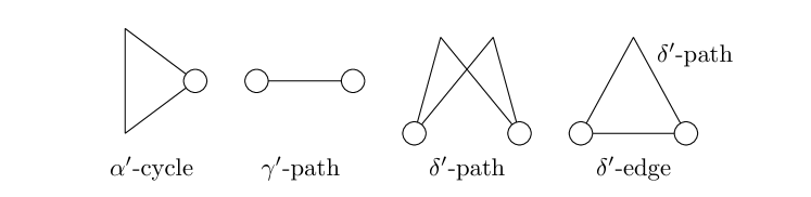
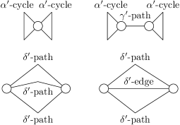
Now we consider the correspondence of $\mathcal{B}\in BG_{k}$ to a basic graph with respect to complete graphs $\{K_{n}\}_{n\geq 1}$. A basic graph $\mathcal{A}$ on $\{K_{n}\}_{n\geq 1}$ consists of the following four types of (minimal) special cycle, paths and edge as in Figure 5. For details, see [12, Section 6]. An example for case $k=2$ is shown in Figure 6.

Figure 5. Four types of special cycle and paths of basic graphs on $\{K_{n}\}_{n\geq 1}$. The circles denote special points.

(a) Basic graph

(b) Multigraph

Figure 6. Example of the case $k=2$ (cf. [12, Section 7]). The mapping $\psi$ transfers each of the basic graphs of 6 to each of the multigraphs of 6.

Recall that $N(n,k)$ is the number of connected $(n,n-1+k)$-graphs on $K_{n}$, which was introduced in Section 1. Let $W_{k},k\geq 1$ be the exponential generating function of $N(n,k)$:

$$W_{k}(x)=\sum_{n=1}^{\infty}N(n,k)\frac{x^{n}}{n!}.$$

Note that $W_{1}(x)$ is the exponential generating function for “unicycles” on $\{K_{n}\}_{n\geq 1}$, which corresponds to $F_{1}(x,x)$ for bipartite graphs.

Proposition 6.6 ([12]).

For $k\geq 1$, $W_{k}(x)$ is expressed by the summation with respect to basic graphs $\mathcal{A}$:

$$W_{k}(x)=\sum_{\mathcal{A}\in BG^{\prime}_{k}}J_{\mathcal{A}}(x)$$

with

$$J_{\mathcal{A}}(x)=\frac{Y^{L^{\prime}(\mathcal{A})}}{g_{\mathcal{A}}(1-Y)^{M^{\prime}(\mathcal{A})}},$$ (6.9)

where $BG^{\prime}_{k}$ is the set of basic graphs on complete graphs having $k$ cycles and $M^{\prime}(\mathcal{A})\leq 3(k-1)$, $L^{\prime}(\mathcal{A})$ and $g_{\mathcal{A}}$ are constants depending only on $\mathcal{A}$.

Lemma 6.7.

For $\mathcal{A}\in BG^{\prime}_{k}$, there exist unique constants $\{\mathfrak{a}^{\prime}_{i}(\mathcal{A})\}_{i=1}^{M^{\prime}},\{\mathfrak{c}^{\prime}_{j}(\mathcal{A})\}_{j=0}^{L^{\prime}-M^{\prime}}$ such that

$$J_{\mathcal{A}}=\sum_{i=1}^{M^{\prime}}\frac{\mathfrak{a}^{\prime}_{i}(\mathcal{A})}{(1-Y)^{i}}+\sum_{j=0}^{L^{\prime}-M^{\prime}}\mathfrak{c}^{\prime}_{j}(\mathcal{A})Y^{j},\ \ \mathfrak{a}^{\prime}_{M^{\prime}}(\mathcal{A})=\frac{1}{g_{\mathcal{A}}}.$$

Proof.

To show the second equation, put $\theta=1-Y$ in (6.9) and apply the binomial expansion to the numerator. ∎

For each $\mathcal{A}\in BG^{\prime}_{k}$ we contract their special cycles and paths and obtain a multigraph $\mathcal{A}^{*}$. Define $\psi:BG^{\prime}_{k}\to MG_{k}$ be the mapping of the contraction. Note that $\psi$ is not injective, but if $\psi(\mathcal{A}_{1})=\psi(\mathcal{A}_{2})=\mathcal{A}^{*}$ for some $\mathcal{A}_{1},\mathcal{A}_{2}$, then the difference of the two graphs is only due to the difference of their $\delta^{\prime}$-paths and $\delta^{\prime}$-edges. Define

$$BG^{\prime}_{k}|_{3(k-1)}:=\{\mathcal{A}\in BG^{\prime}_{k}:M^{\prime}(\mathcal{A})=3(k-1)\}.$$

Let $\psi|_{3(k-1)}$ be the restriction to $BG^{\prime}_{k}|_{3(k-1)}$ of $\psi$, then this mapping is bijective from $BG^{\prime}_{k}|_{3(k-1)}$ to $MG_{k}$ i.e, $\psi|_{3(k-1)}^{-1}(\mathcal{A}^{*})$ is a singleton. Indeed, if $\mathcal{A}^{*}$ has self-loops, replace them to minimal $\alpha^{\prime}$-cycles. Also, if $\mathcal{A}^{*}$ has single edges or multiple edges, replace them to $\gamma^{\prime}$-paths or $\delta^{\prime}$-paths, respectively. By this procedure, we obtain a unique basic graph $\mathcal{A}\in BG^{\prime}_{k}|_{3(k-1)}$, and then $\psi|_{3(k-1)}^{-1}(\mathcal{A}^{*})=\{\mathcal{A}\}$.

6.3. Proof of the asymptotic equality (1.10)

We will prove the asymptotic equality (1.10). Take $\mathcal{B}^{*}\in MG_{k}$ such that there exists $\mathcal{B}\in\phi^{-1}(\mathcal{B}^{*})$ satisfying $M(\mathcal{B})=3(k-1)$. Then, there exist unique $\mathcal{B}_{{\rm id}}\in\phi^{-1}(\mathcal{B}^{*})$ and $\mathcal{A}=\mathcal{A}_{\mathcal{B}^{*}}:=\psi^{-1}|_{3(k-1)}(\mathcal{B}^{*})\in BG^{\prime}_{k}$. Then, we have

$$g_{\mathcal{B}_{{\rm id}}}=g_{\mathcal{A}},$$ (6.10)

because mappings $\phi$ and $\psi$ preserve the connectivity between each of vertices in $\mathcal{B}$ and $\mathcal{A}$, respectively. By Proposition 6.5 and (6.10), we have

$$\sum_{\begin{subarray}{c}\mathcal{B}\in\phi^{-1}(\mathcal{B}^{*})\\ M(\mathcal{B})=3(k-1)\end{subarray}}\mathfrak{a}_{3(k-1)}(\mathcal{B})=\frac{1}{2^{k-1}}\frac{1}{g_{\mathcal{A}}}.$$ (6.11)

From Proposition 6.6, the asymptotic behavior of $\langle x^{n}\rangle W_{k-1}(x)$ is determined by the summation of $J_{\mathcal{A}}(x)$ with respect to $\mathcal{A}$ such that $M^{\prime}(\mathcal{A})=3(k-1)$. Hence, by Lemma 6.7 we have

$$N(n,k) =\langle x^{n}\rangle W_{k}(x)$$

$$\sim\langle x^{n}\rangle\sum_{\mathcal{A}\in BG^{\prime}_{k}|_{3(k-1)}}J_{\mathcal{A}}(x)$$

$$\sim\sum_{\mathcal{A}\in BG^{\prime}_{k}|_{3(k-1)}}\langle x^{n}\rangle\left(\frac{\mathfrak{a}^{\prime}_{3(k-1)}(\mathcal{A})}{(1-Y)^{3(k-1)}}\right)$$

$$=\Bigg{(}\sum_{\mathcal{A}\in BG^{\prime}_{k}|_{3(k-1)}}\frac{1}{g_{\mathcal{A}}}\Bigg{)}t_{n}(3(k-1)),\quad n\to\infty,$$

where $t_{n}(p)$ is the tree polynomials defined by (4.19). On the other hand, by Lemma 6.1, Proposition 6.3, (6.11) and the fact that $\psi|_{3(k-1)}$ is bijective, we have

$$N_{\rm{bi}}(n,k) =\langle x^{n}\rangle F_{k}(x,x)$$

$$\sim\langle x^{n}\rangle\sum_{\mathcal{B}^{*}\in MG_{k}}\sum_{\begin{subarray}{c}\mathcal{B}\in\phi^{-1}(\mathcal{B}^{*})\\ M(\mathcal{B})=3(k-1)\end{subarray}}J_{\mathcal{B}}(x,x)$$

$$\sim\sum_{\mathcal{B}^{*}\in MG_{k}}\sum_{\begin{subarray}{c}\mathcal{B}\in\phi^{-1}(\mathcal{B}^{*})\\ M(\mathcal{B})=3(k-1)\end{subarray}}\langle x^{n}\rangle\left(\frac{\mathfrak{a}_{3(k-1)}(\mathcal{B})}{(1-Y)^{3(k-1)}}\right)$$

$$=\Bigg{(}\sum_{\mathcal{B}^{*}\in MG_{k}}\sum_{\begin{subarray}{c}\mathcal{B}\in\phi^{-1}(\mathcal{B}^{*})\\ M(\mathcal{B})=3(k-1)\end{subarray}}\mathfrak{a}_{3(k-1)}(\mathcal{B})\Bigg{)}t_{n}(3(k-1))$$

$$=\frac{1}{2^{k-1}}\Bigg{(}\sum_{\mathcal{A}\in BG^{\prime}_{k}|_{3(k-1)}}\frac{1}{g_{\mathcal{A}}}\Bigg{)}t_{n}(3(k-1))$$

$$\sim\frac{1}{2^{k-1}}N(n,k),\quad n\to\infty,$$

hence the asymptotic equality (1.10) holds.

References

- [1] A. Cayley. A theorem on trees. Quart. J. Math. 23 (1889), 376–378.
- [2] M. Drmota and R. Kutzelnigg. Precise analysis of cuckoo hashing. ACM Trans. on Algorithms 8 (2012), 1–36.
- [3] P. Flajolet and R. Sedgewick. Analytic Combinatorics. Cambridge University Press, Cambridge, UK, 2009.
- [4] P. Flajolet and R. Sedgewick. An Introduction to the Analysis of Algorithms, Second Edition. Addison-Wesley Professional, 2013.
- [5] S. Janson, D. E. Knuth, T. Luczak, and B. Pittel. The birth of the giant component. Random Struct. Algorithms 4 (1993), 233–358.
- [6] P. M. Kayll and D. Perkins. Combinatorial proof of an Abel-type identity. J. Combin. Math. Combin. Comput. 70 (2009), 33–40.
- [7] D. E. Knuth and B. Pittel. A recurrence related to trees. Proc. Am. Math. Soc. 105 (1989), 335–349.
- [8] R. Kutzelnigg. Random graphs and Cuckoo Hashing. A precise average case analysis of Cuckoo Hashing and some parameters of sparse random graphs. Sudwestdeutscher Verlag für Hochschuleschriften, 2009.
- [9] A. Rényi. On connected graphs I. Pubf. Math. Inst. Hungarian Acad. Sci. 4 (1959), 385–388.
- [10] J. Riordan. Combinatorial Identities. Wiley Series in Probability and Mathematical Statistics, Wiley, 1968.
- [11] H. I. Scoins. The number of trees with nodes of alternate parity. Proc. Cambridge Philos. Soc. 58 (1962), 12–16.
- [12] E. M. Wright. The number of connected sparsely edged graphs. J. Graph Theory 1 (1977), 317–330.