Dataset Obfuscation: Its Applications to and Impacts on Edge Machine Learning

Abstract.

Obfuscating a dataset by adding random noises to protect the privacy of sensitive samples in the training dataset is crucial to prevent data leakage to untrusted parties for edge applications. We conduct comprehensive experiments to investigate how the dataset obfuscation can affect the resultant model weights - in terms of the model accuracy, Frobenius-norm (F-norm)-based model distance, and level of data privacy - and discuss the potential applications with the proposed Privacy, Utility, and Distinguishability (PUD)-triangle diagram to visualize the requirement preferences. Our experiments are based on the popular MNIST and CIFAR-10 datasets under both independent and identically distributed (IID) and non-IID settings. Significant results include a trade-off between the model accuracy and privacy level and a trade-off between the model difference and privacy level. The results indicate broad application prospects for training outsourcing in edge computing and guarding against attacks in Federated Learning among edge devices.

1. Introduction

Artificial Intelligence (AI) has evolved for decades and the capability of machine learning has become one of the core components in many applications in human daily life, including edge computing networks (edge-1, ; edge-2, ). Recently, formulating the AI ethics and building Responsible AI have been attracting increasing attention from industry and academia to ensure processes being legitimate, secure, and ethical for everyone involved.

Data privacy is one of the hotspots with various privacy-preserving solutions being proposed in terms of designing privacy-aware machine learning algorithms and platforms (DLDP2016CCS, ; PPDP2015ACM, ; hesamifard2018privacy, ; 197247, ) or implementing cryptographic algorithms, such as homomorphic encryption, to encrypt the dataset (cryptoeprint:2014/331, ) prior to data disclosure. However, the privacy-aware machine learning algorithms address only the “hidden trees in a forest” problem by obfuscating the query results, and cannot prevent data leakage for each piece of data samples. On the other hand, homomorphic encryption is computationally intensive  (10.1145/3214303, ) and prohibitive for edge applications, and has to be carefully crafted with respect to different learning algorithms with weak generality (noisy-dataset, ).

Obfuscating a dataset using random noises recently came to the scene due to the increasing importance of data privacy in edge networks (edge-privacy, ), particularly the training dataset privacy, in machine learning processes where edge-edge or edge-cloud dataset sharing is essential. A general practice of preserving data privacy is to add random noise to datasets during the data sharing to preserve the data privacy as one needs no compulsory presumptions about the trust between him/her and the data receivers. The most relevant study evaluates only the impacts of obfuscation on model prediction accuracy (noisy-dataset, ), with no mention of either the model distance or the data utility which can outweigh the accuracy in many application scenarios. The F-norm-based model distance has been widely used, and its importance has appeared in many areas. A typical example is applying Proof-of-Learning (PoL) (9519402, ) in Federated Learning (FL), where the Frobenius-norm (F-norm) is used to evaluate the model distance between two versions of the model originating from the raw and obfuscated datasets, respectively. Another example is the Multi-Krum aggregation (multi-krum, ) in FL can be byzantine-fault-tolerant by removing the model outliers in terms of F-norm. Therefore, we consider assessing the F-norm-based model distance under dataset obfuscation, which has yet been learned in existing studies, is essential and can help to understand the nature of dataset obfuscation in the above applications, thus encouraging the advancement of privacy-preserving protocols.

The goal of this paper is to comprehensively investigate the impacts of noise-based dataset obfuscation on the trained models. In this paper, we extend comprehensive experiments regarding the dataset obfuscation in machine learning, to analyze in-depth the impacts on the resultant models and explore potential application scenarios in edge networks. The key contributions of this paper are as follows.

1. We determine a generic obfuscation model with various metrics considered over a training dataset.

2. We carry out various types of experiments over the MNIST (726791, ) and CIFAR-10 (krizhevsky2009learning, ) datasets under both independent and identically distributed (IID) and non-IID conditions with a wide range of noise settings.

3. We discuss the challenges and potential applications in edge networks based upon the experimental results, including training outsourcing and Federated Learning (FL), with a new visualization tool, named Privacy, Utility, and Distinguishability (PUD)-triangle diagram.

The experiments show that the model accuracy declines with the increase of noise level. The increasing noise level also enlarges the model difference between feeding a raw dataset and its obfuscated version, thus weakening the training reproducibility. Also, the disguisability of fake datasets becomes stronger with the increase of noise level due to the subequal model differences. The resultant observation indicates the existence of a balanced stable point at which all metrics can be acceptable for real applications, including training outsourcing on edge computing and guarding against attacks in FL among edge devices.

The rest of the paper is organized as follows. The related works are given in Section 2. Section 3 provides the background. The experiment settings and results are shown in Section 4, followed by discussions in Section 5. Section 6 concludes the paper.

2. Related Work

Protecting privacy in machine learning has attracted wide attention and spawned many approaches in terms of collaborative learning where datasets are locally used at edge devices with only small subsets of parameters shared (PPDP2015ACM, ), obfuscating the local model parameters by using random noise or differential privacy at edge devices (8843942, ), adopting homomorphic encryption to encrypt data samples (hesamifard2018privacy, ), etc.

This paper focuses on protecting dataset privacy in tasks where sharing datasets is essential between edges or between edge and cloud. Authors of (noisy-dataset, ) focus on the training outsourcing and propose an OBFUSCATE function to obfuscate training datasets before the disclosure. The function adds random noises to data samples or augments datasets with new samples to protect the dataset privacy. The authors also show that training upon the obfuscated dataset can preserve the model accuracy. Our paper conducts more comprehensive experiments to investigate impacts on not only the model accuracy, but also the model difference under both IID and non-IID settings (the latter of which is yet to be considered in existing studies). We explore and discuss real-world applications in edge computing which can take advantage of dataset obfuscation by also establishing the PUD-triangle to visualize the requirement preferences.

3. Overview of Dataset Obfuscation

This section introduces important definitions in each step of the obfuscation model and key performance used to evaluate the impacts on the resultant models in the crafted experiments.

• Model Training

Given a model $\mathcal{M}$ and a dataset $T=\{t_{i},l_{i}\}$ with $t_{i}$ being the $i$-th sample in the dataset and $l_{i}$ being the label of the sample, the model weights $W$ can be trained with the training function $\mathcal{F}$.

(1) $$W=\mathcal{F}(T,\mathcal{M}).$$

The trained weights $W$ can be tested on a testing dataset $T_{e}$ and evaluated with the model prediction accuracy $\mathcal{A}(W)$.

• Data Obfuscation

We consider a uniform obfuscation of training data where IID noises are added to the training data, denoted by $T^{\prime}=\text{ }\mathcal{O}(T)$. The obfuscation function $\mathcal{O}(T)$ can be given by

(2) $$\begin{split}&t_{ij}^{\prime}=\text{ }t_{ij}+\delta,\forall\text{ }i\text{ and }j,\ \delta\sim\mathcal{N}(0,\sigma^{2});\\ &l_{i}^{\prime}=\text{ }l_{i};\end{split}$$

where $t_{ij}$ is the $j$-th feature of $t_{i}$, and $t^{\prime}_{ij}$ is the obfuscated version in $T^{\prime}$. Labels, i.e., $l_{i}^{\prime}$ and $l_{i}$, remain the same after data obfuscation. $\delta\sim\mathcal{N}(0,\sigma^{2})$ stands for the added Gaussian noise. The mean of the Gaussian noise is zero to ensure data utility. Here we consider all training data is obfuscated by setting $R=1$, where $R$ is the proportion of obfuscated data in the training dataset.

• Model Difference

We use the F-norm, i.e., $\|\cdot\|_{\text{F}}$, to measure the difference between two model weights, as given by

(3) $$\begin{split}\mathcal{D}(W_{i},W_{j})&=\|W_{i}-W_{j}\|_{\text{F}}=\sqrt{\sum_{k}|w_{ik}-w_{jk}|^{2}},\end{split}$$

where $w_{ik}$ and $w_{jk}$ are the $k$-th entries of $W_{i}$ and $W_{j}$, respectively.

4. Experiments

In this section, we experimentally evaluate the impacts of adding random noise to training datasets on the resultant models. Experiments cover a range of Gaussian standard deviations and various IID and non-IID dataset settings.

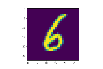
(a) $\sigma=0$

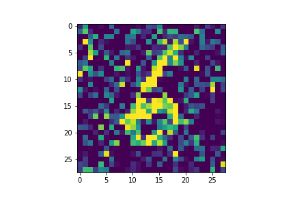
(b) $\sigma=0.4$

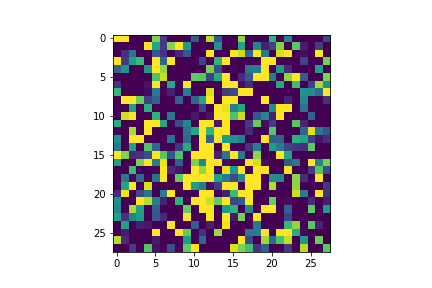
(c) $\sigma=0.8$

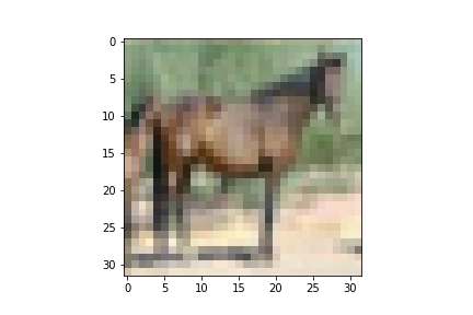
(d) $\sigma=0$

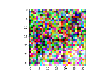
(e) $\sigma=0.4$

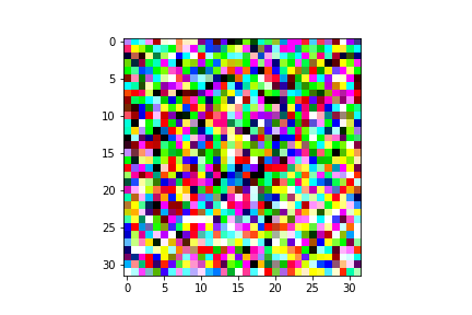
(f) $\sigma=0.8$

Figure 1. Obfuscated MNIST (a, b, c) and CIFAR-10 (d, e, f).

4.1. Experiment Framework

4.1.1. System Settings

We train classification models using popular MNIST (10 labels and 60,000 training examples) and CIFAR-10 (10 labels and 50,000 training examples) datasets. Each of the datasets is randomly split into a global training dataset $T_{t}$ with 90% data and a testing dataset $T_{e}$ with the remaining 10% data. The classification model is a standard Convolutional Neural Network (CNN) with six convolution layers and three max-pooling layers, named as $\mathcal{M}_{cnn}$. An initial model with random weights is used across all experiments. $\mathcal{M}_{cnn}$ is trained with 180 epochs and a learning rate of 0.0001 on both datasets. The batch sizes for the training on MNIST and CIFAR-10 are 128 and 64, respectively.

We conduct the experiments upon Ubuntu 20.04.3 with TensorFlow 2.7.0 GPU kernel in Python 3.7. The training runs on a local machine with the following specifications: 2x Intel(R) Xeon(R) Gold 6138 CPU @ 2.00GHz, 256GB RAM, 16TB of Disk Space, and 8x NVIDIA A100 40GB.

4.1.2. Training Dataset Settings

We generate the training datasets from the global $T_{t}$ on IID and non-IID features, respectively, to show the impacts of training data on trained models. In the case of a non-IID dataset, we follow the non-IID data setting in (li2021federated, ) and consider Label-Skew-based and Quantity-Skew-based non-IID cases. We use “S-$\mathcal{X}$-$\mathcal{Y}$-$\mathcal{Z}$” to represent the sampling settings of training datasets.

• Label degree $\mathcal{X}$: The dataset covers $\lfloor\mathcal{CX}\rfloor$ of the total $C$ labels, where $C=10$ for both datasets in this paper.

• Label overlapping ratio $\mathcal{Y}$: The dataset and its counterpart cover the same $\lfloor C\mathcal{X}\mathcal{Y}\rfloor$ labels.

• Sampling ratio $\mathcal{Z}$: The dataset samples the entries of $T_{t}$ with ratio $\mathcal{Z}$ for each of the covered labels. The dataset contains $\mathcal{X}\mathcal{Z}|T_{t}|$ entries, where $|\cdot|$ gives cardinality.

4.2. Experiment Results and Evaluations

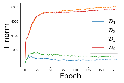
(a) F-norm

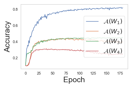
(b) Accuracy

Figure 2. The dynamic F-norm and accuracy over epochs.

A first look at the data obfuscation over MNIST and CIFAR-10 by adding the random Gaussian noises is shown in Fig. 1.

We show the dynamics of model difference and model accuracy during training with CIFAR-10 in Fig. 2 with setup in Table 1. A reference dataset $T_{r}$ is sampled from a global $T_{t}$ with setting S-1-1-0.5, i.e., covering all labels and containing half of the global data. $T_{r}$ is also used as $T_{1}$, i.e., $T_{1}=T_{r}$, and obfuscated with $\sigma=1$ for $T_{o,2}$, i.e., $T_{o,2}=\mathcal{O}(T_{r}),\sigma=1$. Dataset $T_{3}$ is sampled from $T_{t}$ with setting S-0.5-1-1, i.e., covering half labels and containing all entries with the covered labels. $T_{o,4}$ is obfuscated $T_{3}$, i.e., $T_{o,4}=\mathcal{O}(T_{3})$, $\sigma=1$. All datasets contain $0.5|T_{t}|$ entries. $W_{r}$ and $W_{i}$ can then be obtained by training the initial model on datasets. Next, the model distance can be computed via $\mathcal{D}_{i}=\mathcal{D}(W_{r},W_{i})$. Models are evaluated on $T_{e}$ for accuracy $\mathcal{A}(W)$. Results in Fig. 2 show the convergence of both F-norm and accuracy over all (non-)IID and (non-)obfuscated settings. Note that the number of epochs used in all the experiments in this paper complies with that of Fig. 2.

We proceed to conduct four experiments over the MNIST and CIFAR-10 datasets from the following perspectives.

Exp-1 ($\mathcal{A}(W)$ vs. $\sigma$ with different label degrees) - Figs. 3(a) and 3(b) with setup in Table 2. The model weight $W_{1,1}$ is trained on the obfuscated dataset $T_{o,1,1}=\mathcal{O}(T_{1,1})$ where $T_{1,1}$ is sampled from $T_{t}$ with setting S-1-1-0.5, and then evaluated on $T_{e}$ for $\mathcal{A}(W_{1,1})$. $\mathcal{A}(W_{1,2})$ and $\mathcal{A}(W_{1,3})$ are obtained in the same way with settings S-0.8-1-0.625 and S-0.5-1-1, respectively. All the datasets contain $0.5|T_{t}|$ entries.

Table 1. Experiment setup for Fig. 2

Dataset	Composition	Size
$T_{t}$	90% of CIFAR-10 dataset	45,000
$T_{e}$	Rest 10% CIFAR-10 dataset	5,000
$T_{1}$ ($T_{r}$)	Sampled from $T_{t}$, with $\mathcal{X}=1$, $\mathcal{Y}=1$, $\mathcal{Z}=0.5$	0.5$|T_{t}|$
$T_{o,2}$	$\mathcal{O}(T_{1})$ with $\sigma=1$	$0.5|T_{t}|$
$T_{3}$	Sampled from $T_{t}$ with $\mathcal{X}=0.5$, $\mathcal{Y}=1$, $\mathcal{Z}=1$	$0.5|T_{t}|$
$T_{o,4}$	$\mathcal{O}(T_{3})$ with $\sigma=1$	$0.5|T_{t}|$
Figures	Operations	Outputs
Fig. 2(a)	Train $\mathcal{M}_{cnn}$ on $T_{r}$, $T_{1}$, $T_{o,2}$, $T_{3}$, $T_{o,4}$	$W_{r}$, $W_{1}$, $W_{2}$, $W_{3}$, $W_{4}$
	Calculate $\mathcal{D}(\cdot)$ between $W_{r}$ and [$W_{1}$, $W_{2}$, $W_{3}$, $W_{4}$]	$D_{1}$, $D_{2}$, $D_{3}$, $D_{4}$
Fig. 2(b)	Evaluate model accuracy over $T_{e}$	$\mathcal{A}(W_{1})$, $\mathcal{A}(W_{2})$, $\mathcal{A}(W_{3})$, $\mathcal{A}(W_{4})$

Table 2. Experiment setup for Exp-1

Dataset	Composition	Size
$T_{t}$	90% of MNIST/CIFAR-10 dataset	54,000/45,000
$T_{e}$	Rest 10% MNIST/CIFAR-10 dataset	6,000/5,000
$T_{1,1}$	Sampled from $T_{t}$, with $\mathcal{X}=1$, $\mathcal{Y}=1$, $\mathcal{Z}=0.5$	0.5$|T_{t}|$
$T_{1,2}$	Sampled from $T_{t}$ with $\mathcal{X}=0.8$, $\mathcal{Y}=1$, $\mathcal{Z}=0.625$	$0.5|T_{t}|$
$T_{1,3}$	Sampled from $T_{t}$ with $\mathcal{X}=0.5$, $\mathcal{Y}=1$, $\mathcal{Z}=1$	$0.5|T_{t}|$
Figures	Operations	Outputs
Fig. 3(a) MNIST	Execute $\mathcal{O}(\cdot)$ on $T_{1,1}$, $T_{1,2}$, and $T_{1,3}$	$T_{o,1,1}$, $T_{o,1,2}$, $T_{o,1,3}$
	Train $\mathcal{M}_{cnn}$ on $T_{o,1,1}$, $T_{o,1,2}$, $T_{o,1,3}$	$W_{1,1}$, $W_{1,2}$, and $W_{1,3}$
	Evaluate model accuracy over $T_{e}$	$\mathcal{A}(W_{1,1})$, $\mathcal{A}(W_{1,2})$, $\mathcal{A}(W_{1,3})$
Fig. 3(b) CIFAR-10	Same as above	Same as above

Exp-2 ($\mathcal{A}(W)$ vs. $\sigma$ with different dataset sizes) - Figs. 3(c) and 3(d) with setup in Table 3. The model weight $W_{2,1}$ is trained on the obfuscated dataset $T_{o,2,1}=\mathcal{O}(T_{2,1})$ where $T_{2,1}$ is sampled from $T_{t}$ with setting S-0.8-1-1, and then evaluated on $T_{e}$ for $\mathcal{A}(W_{2,1})$. $\mathcal{A}(W_{2,2})$ and $\mathcal{A}(W_{2,3})$ are obtained in the same way with settings S-0.8-1-0.5 and S-0.8-1-0.1, respectively. $T_{2,1}$, $T_{2,2}$ and $T_{2,3}$ cover the same eight labels and contain $0.8|T_{t}|$, $0.4|T_{t}|$, and $0.08|T_{t}|$ entries, respectively.

Table 3. Experiment setup for Exp-2

Dataset	Composition	Size
$T_{t}$	90% of MNIST/CIFAR-10 dataset	54,000/45,000
$T_{e}$	Rest 10% MNIST/CIFAR-10 dataset	6,000/5,000
$T_{2,1}$	Sampled from $T_{t}$, with $\mathcal{X}=0.8$, $\mathcal{Y}=1$, $\mathcal{Z}=1$	0.8$|T_{t}|$
$T_{2,2}$	Random 50% data of $T_{2,1}$	$0.4|T_{t}|$
$T_{2,3}$	Random 10% data of $T_{2,1}$	$0.08|T_{t}|$
Figures	Operations	Outputs
Fig. 3(c) MNIST	Execute $\mathcal{O}(\cdot)$ on $T_{2,1}$, $T_{2,2}$, and $T_{2,3}$	$T_{o,2,1}$, $T_{o,2,2}$, $T_{o,2,3}$
	Train $\mathcal{M}_{cnn}$ on $T_{o,2,1}$, $T_{o,2,2}$, $T_{o,2,3}$	$W_{2,1}$, $W_{2,2}$, and $W_{2,3}$
	Evaluate model accuracy over $T_{e}$	$\mathcal{A}(W_{2,1})$, $\mathcal{A}(W_{2,2})$, $\mathcal{A}(W_{2,3})$
Fig. 3(d) CIFAR-10	Same as above	Same as above

Exp-3 ($\mathcal{D}(W_{r},W_{o})$ vs. $\sigma$ with different label degrees) - Figs. 4(a) and 4(b) with setup in Table 4. $W_{r}$ is obtained by training reference datasets $T_{r}$ without any noise, while $W_{o}$ is from the obfuscated datasets $T_{o}$. Three sampling settings are designed to capture the impact of noise on models from IID datasets under different label degrees. Setting S-1-1-0.25 is employed for $\mathcal{D}_{3,1}$ and $\mathcal{D}_{3,2}$. $\mathcal{D}_{3,1}=\mathcal{D}(W_{r,3,1},W_{o,3,1})$, where $W_{r,3,1}$ is from dataset $T_{r,3,1}$ sampled from $T_{t}$ with setting S-1-1-0.25. The reference dataset is also used for the obfuscated dataset for $W_{o,3,1}$, i.e., $T_{o,3,1}$=$O(T_{r,3,1})$. In terms of $\mathcal{D}_{3,2}=\mathcal{D}(W_{r,3,1},W_{o,3,2})$, $T_{o,3,2}=O(T_{3,2})$ where $T_{3,2}$ is sampled from $T_{t}$ following the same setting S-1-1-0.25. All the datasets for $\mathcal{D}_{3,1}$ and $\mathcal{D}_{3,2}$ cover all the ten labels. $\mathcal{D}_{3,3}$ and $\mathcal{D}_{3,4}$ are obtained with setting S-0.5-1-0.5, in which all datasets cover the first five labels. All datasets in Exp-3 contain $0.25|T_{t}|$ entries.

Table 4. Experiment setup for Exp-3

Dataset	Composition	Size
$T_{t}$	90% of MNIST/CIFAR-10 dataset	54,000/45,000
$T_{e}$	Rest 10% MNIST/CIFAR-10 dataset	6,000/5,000
$T_{3,1}$ ($T_{r,3,1}$)	Sampled from $T_{t}$, with $\mathcal{X}=1$, $\mathcal{Y}=1$, $\mathcal{Z}=0.25$	$0.25|T_{t}|$
$T_{3,2}$	Sampled from $T_{t}$, with the same setting and labels of $T_{3,1}$	$0.25|T_{t}|$
$T_{3,3}$ ($T_{r,3,2}$)	Sampled from $T_{t}$, with $\mathcal{X}=0.5$, $\mathcal{Y}=1$, $\mathcal{Z}=0.5$	$0.25|T_{t}|$
$T_{3,4}$	Sampled from $T_{t}$, with the same setting and labels of $T_{3,3}$	$0.25|T_{t}|$
Figures	Operations	Outputs
Fig. 4(a) MNIST	Execute $\mathcal{O}(\cdot)$ on $T_{3,1}$, $T_{3,2}$, $T_{3,3}$, and $T_{3,4}$ with a varying $\sigma$	$T_{o,3,1}$, $T_{o,3,2}$, $T_{o,3,3}$, $T_{o,3,4}$
	Train $\mathcal{M}_{cnn}$ on $T_{r,3,1}$, $T_{r,3,2}$, $T_{o,3,1}$, $T_{o,3,2}$, $T_{o,3,3}$, and $T_{o,3,4}$	$W_{r,3,1}$, $W_{r,3,2}$, $W_{o,3,1}$, $W_{o,3,2}$, $W_{o,3,3}$, $W_{o,3,4}$
	Calculate $\mathcal{D}(\cdot)$ between $W_{r,3,1}$ and [$W_{o,3,1}$, $W_{o,3,2}$]	$\mathcal{D}_{3,1}$, $\mathcal{D}_{3,2}$
	Calculate $\mathcal{D}(\cdot)$ between $W_{r,3,2}$ and [$W_{o,3,3}$, $W_{o,3,4}$]	$\mathcal{D}_{3,3}$, $\mathcal{D}_{3,4}$
Fig. 4(b) CIFAR-10	Same as above	Same as above

Exp-4 ($\mathcal{D}(W_{r},W_{o})$ vs. $\sigma$ with different label overlapping ratios) - Figs. 4(c) and 4(d) with setup in Table 5. $\mathcal{D}_{4,1}=\mathcal{D}(W_{r,4,1},W_{o,4,1})$, where $W_{r,4,1}$ is trained from dataset $T_{r,4,1}$ that is sampled from $T_{t}$ with setting S-0.5-1-0.5 and covers labels 0, 1, 2, 3 and 4. The reference dataset is also employed for the obfuscated dataset $W_{o,4,1}$, i.e., $T_{o,4,1}$=$O(T_{r,4,1})$, and the reference dataset in Exp-4. In terms of $\mathcal{D}_{4,2}=\mathcal{D}(W_{r,4,1},W_{o,4,2})$, $T_{o,4,2}$ is an obfuscated $T_{4,2}$ that is sampled from $T_{t}$ with setting S-0.5-0.5-0.5 and covers labels 3, 4, 5, 6 and 7. For $\mathcal{D}_{4,3}=\mathcal{D}(W_{r,4,1},W_{o,4,3})$, $T_{o,4,3}$ is an obfuscated $T_{4,3}$ that is sampled from $T_{t}$ with setting S-0.5-0.1-0.5 and covers labels 4, 5, 6, 7 and 8. All datasets contain $0.25|T_{t}|$ entries.

Table 5. Experiment setup for Exp-4

Dataset	Composition	Size
$T_{t}$	90% of MNIST/CIFAR-10 dataset	54,000/45,000
$T_{e}$	Rest 10% MNIST/CIFAR-10 dataset	6,000/5,000
$T_{4,1}$ ($T_{r,4,1}$)	Sampled from $T_{t}$, with $\mathcal{X}=0.5$, $\mathcal{Y}=1$, $\mathcal{Z}=0.5$, covering labels 0-4	$0.25|T_{t}|$
$T_{4,2}$	Sampled from $T_{t}$, with $\mathcal{X}=0.5$, $\mathcal{Y}=0.4$, $\mathcal{Z}=0.5$, covering labels 3-7	$0.25|T_{t}|$
$T_{4,3}$	Sampled from $T_{t}$, with $\mathcal{X}=0.5$, $\mathcal{Y}=0.2$, $\mathcal{Z}=0.5$, covering labels 4-8	$0.25|T_{t}|$
Figures	Operations	Outputs
Fig. 4(c) MNIST	Execute $\mathcal{O}(\cdot)$ on $T_{4,1}$, $T_{4,2}$, and $T_{4,3}$ with a varying $\sigma$	$T_{o,4,1}$, $T_{o,4,2}$, $T_{o,4,3}$
	Train $\mathcal{M}_{cnn}$ on $T_{r,4,1}$, $T_{o,4,1}$, $T_{o,4,2}$, and $T_{o,4,3}$	$W_{r,4,1}$, $W_{o,4,1}$, $W_{o,4,2}$, $W_{o,4,3}$
	Calculate $\mathcal{D}(\cdot)$ between $W_{r,4,1}$ and [$W_{o,4,1}$, $W_{o,4,2}$, $W_{o,4,3}$]	$\mathcal{D}_{4,1}$, $\mathcal{D}_{4,2}$, $\mathcal{D}_{4,3}$
Fig. 4(d) CIFAR-10	Same as above	Same as above

Exp-5 ($\mathcal{D}(W_{r},W_{o})$ vs. $\sigma$ with different dataset sizes) - Figs. 5(a) and 5(b) with setup in Table 6. $\mathcal{D}_{5,1}=\mathcal{D}(W_{r,5,1},W_{o,5,1})$, where $W_{r,5,1}$ is trained on the dataset $T_{r,5,1}$ that is sampled from $T_{t}$ with setting S-1-1-0.5 and contains $0.5|T_{t}|$ entries. The reference dataset is also used for the obfuscated dataset $W_{o,5,1}$, i.e., $T_{o,5,1}$=$O(T_{r,5,1})$, and the other reference datasets in this experiment, i.e., $T_{r,5,3}=T_{r,5,2}=T_{r,5,1}$. In terms of $\mathcal{D}_{5,2}$, $T_{o,5,2}$ is an obfuscated $T_{5,2}$ that is sampled from $T_{t}$ with setting S-1-1-0.25 and contains $0.25|T_{t}|$ entries. For $\mathcal{D}_{5,3}$, $T_{o,5,3}$ is sampled from $T_{t}$ with setting S-1-1-0.05 and contains $0.05|T_{t}|$ entries.

Table 6. Experiment setup for Exp-5

Dataset	Composition	Size
$T_{t}$	90% of MNIST/CIFAR-10 dataset	54,000/45,000
$T_{e}$	Rest 10% MNIST/CIFAR-10 dataset	6,000/5,000
$T_{5,1}$ ($T_{r,5,1}$)	Sampled from $T_{t}$, with $\mathcal{X}=1$, $\mathcal{Y}=1$, $\mathcal{Z}=0.5$	$0.5|T_{t}|$
$T_{5,2}$	Sampled from $T_{t}$, with $\mathcal{X}=1$, $\mathcal{Y}=1$, $\mathcal{Z}=0.25$	$0.25|T_{t}|$
$T_{5,3}$	Sampled from $T_{t}$, with $\mathcal{X}=1$, $\mathcal{Y}=1$, $\mathcal{Z}=0.05$	$0.05|T_{t}|$
Figures	Operations	Outputs
Fig. 5(a) MNIST	Execute $\mathcal{O}(\cdot)$ on $T_{5,1}$, $T_{5,2}$, and $T_{5,3}$ with a varying $\sigma$	$T_{o,5,1}$, $T_{o,5,2}$, $T_{o,5,3}$
	Train $\mathcal{M}_{cnn}$ on $T_{r,5,1}$, $T_{o,5,1}$, $T_{o,5,2}$, and $T_{o,5,3}$	$W_{r,5,1}$, $W_{o,5,1}$, $W_{o,5,2}$, $W_{o,5,3}$
	Calculate $\mathcal{D}(\cdot)$ between $W_{r,5,1}$ and [$W_{o,5,1}$, $W_{o,5,2}$, $W_{o,5,3}$]	$\mathcal{D}_{5,1}$, $\mathcal{D}_{5,2}$, $\mathcal{D}_{5,3}$
Fig. 5(b) CIFAR-10	Same as above	Same as above

Fig. 3 shows the decrease of the model accuracy with the increase of the noise level. The less diversified labels a training dataset contains, the lower accuracy the model can achieve over a fully-labeled testing dataset ($\mathcal{X}=1$), as shown in Figs. 3(a) and 3(b). On the other hand, the models containing more data samples across covered labels can be more resistant to the adverse effect of obfuscation on the model accuracy, as shown in Figs. 3(c) and 3(d). This indicates that the accumulation of knowledge from the obfuscated samples is useful for recognizing the correct patterns.

It can be found in Fig. 4 that the F-norm $\mathcal{D}(W_{r},W_{o})$ increases with the noise level. This reflects that the obfuscated samples lead the model into a different direction of gradient descent, thus weakening the training reproducibility. In Figs. 4(a) and 4(b), we conduct two types of comparisons:

• A cross-comparison about the F-norm between points with different reference datasets ($\mathcal{D}_{3,1}$ and $\mathcal{D}_{3,2}$ vs. $\mathcal{D}_{3,3}$ and $\mathcal{D}_{3,4}$). Results show that, in terms of F-norm, $\mathcal{D}_{3,3}$ and $\mathcal{D}_{3,4}$ are greater than $\mathcal{D}_{3,1}$ and $\mathcal{D}_{3,2}$ when the noise is large over a relatively simpler training task MNIST but behaves in the opposite way over the CIFAR-10 dataset. Despite having more labels (larger $\mathcal{X}$) leads to higher model privacy as revealed in Figs. 3(c) and 3(d), having a larger F-norm with a higher model accuracy implies the existence of multiple optima.

• A comparison between points with the same reference datasets ($\mathcal{D}_{3,1}$ vs. $\mathcal{D}_{3,2}$ and $\mathcal{D}_{3,3}$ vs. $\mathcal{D}_{3,4}$). Results show that the gap of either comparison becomes indistinguishable in both two groups with the noise level increasing to $\sigma\approx 0.4$. In addition, the more diversified labels a dataset contains, the harder it can be discriminable from the other dataset, and the weaker the model can be resistant to the adverse effect of obfuscation on the model difference.

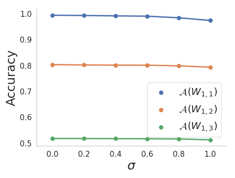
(a) Exp-1 over MNIST

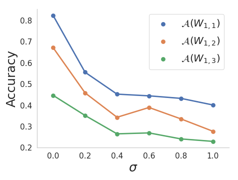
(b) Exp-1 over CIFAR-10

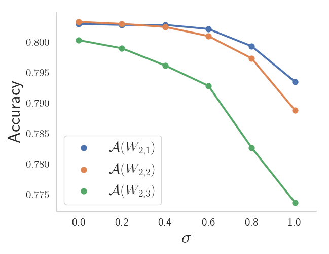
(c) Exp-2 over MNIST

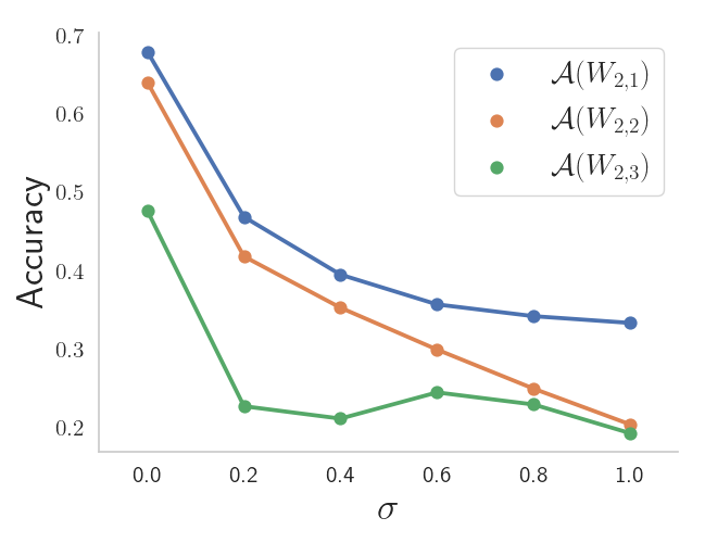
(d) Exp-2 over CIFAR-10

Figure 3. Model prediction accuracy over the testing dataset $T_{e}$ along with the increase of noise level $\sigma$ under different label degrees $\mathcal{X}$ and sampling ratios $\mathcal{Z}$ in MNIST and CIFAR-10 datasets, respectively. The $x$-axis is $\sigma$, and the $y$-axis gives the accuracy.

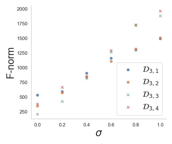
(a) Exp-3 over MNIST

(b) Exp-3 over CIFAR-10

(c) Exp-4 over MNIST

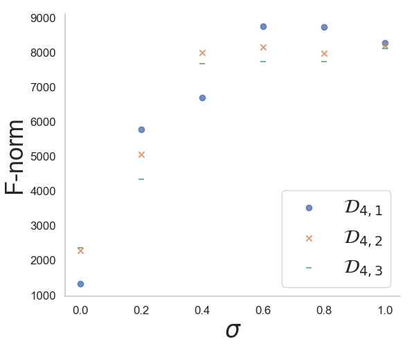
(d) Exp-4 over CIFAR-10

Figure 4. F-norm-based model difference between models trained from reference datasets without noise and obfuscated datasets along with the increase of noise level $\sigma$. The $x$-axis is $\sigma$ for Gaussian noise, and the $y$-axis gives the F-norm values.

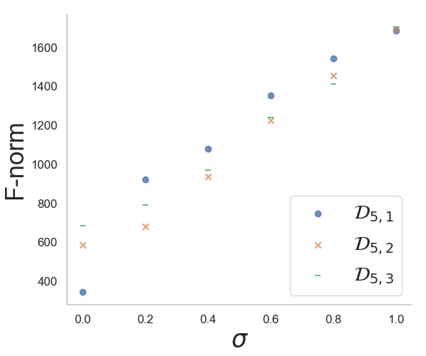
(a) Exp-5 over MNIST

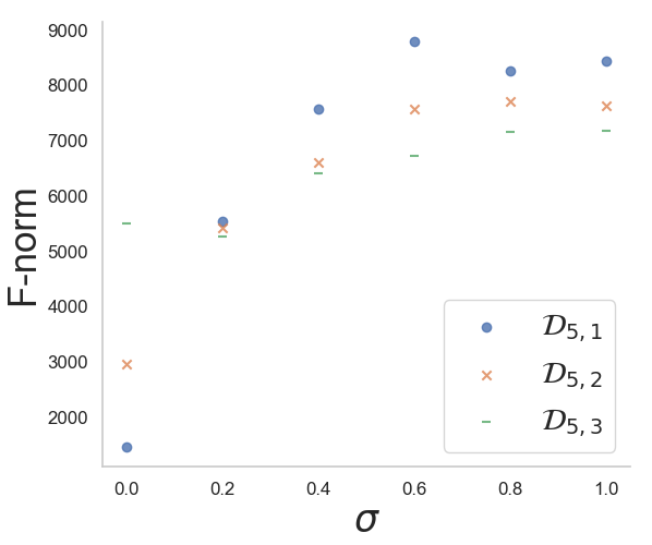
(b) Exp-5 over CIFAR-10

Figure 5. Model difference along with the increase of noise level $\sigma$. The $x$-axis is $\sigma$ for Gaussian noise, and the $y$-axis gives the F-norm values.

In Figs. 4(c) and 4(d), the gaps between the reference points, $\mathcal{D}_{4,1}$, and $\mathcal{D}_{4,2}$, and $\mathcal{D}_{4,3}$ at each given noise level are considered. The experiments on both MNIST and CIFAR-10 show that the gaps narrow down as the noise level increases. Given the same noise level, $\mathcal{D}_{4,3}$ tends to be more discriminable from $\mathcal{D}_{4,1}$ than $\mathcal{D}_{4,2}$ due to the lower label overlapping ratios $\mathcal{Y}$ between $\mathcal{D}_{4,1}$ and $\mathcal{D}_{4,3}$. Also, having such a lower $\mathcal{Y}$ can be more resistant to the impacts of obfuscation on the model difference, given that $\mathcal{X}$s are identical.

Figs. 5(a) and 5(b) are learned in concert with Figs. 3(c) and 3(d) in terms of the sampling ratio $\mathcal{Z}$. Given a certain number of epochs and identical $\mathcal{X}$s and $\mathcal{Y}$s, a smaller $\mathcal{Z}$ leads to a smaller F-norm at a high level of obfuscation. This is because $\mathcal{Z}$ corresponds to the size of dataset and is proportional to the number of learning steps per epoch with identical batch sizes, thus reducing the impacts of obfuscation and making $W_{o,5,2}$ and $W_{o,5,3}$ even closer to $W_{o,5,1}$ than $W_{r,5,1}$ is with $T_{o,5,1}$=$T_{r,5,1}$.

5. Discussions

We discuss challenges of implementing dataset obfuscation, and explore real-world applications particularly on edge networks in this section. We first highlight the following three definitions,

• Privacy: the degree to which a training dataset $T_{tr}$ is confused with $T_{tr}^{\prime}$ to prevent data leakage;

• Utility: the degree to which the obfuscated dataset $T_{tr}^{\prime}$ can be utilized to allow the local model to achieve acceptable model prediction accuracy upon the testing dataset;

• Distinguishability: the degree to which the F-norm gap $\Delta$ associated with a raw training dataset $T_{tr}^{i}$ between its obfuscated dataset $T_{tr}^{i^{\prime}}$ and a different dataset $T_{tr}^{j^{\prime}}$ with the same level of obfuscation.

  (4) $$\Delta=|\mathcal{D}(W_{T_{tr}^{i}},W_{T_{tr}^{i^{\prime}}})-\mathcal{D}(W_{T_{tr}^{i}},W_{T_{tr}^{j^{\prime}}})|,\ \text{where }i\neq j.$$

The PUD-triangle refers to the levels in terms of the degree and nature of Privacy, Utility, and Distinguishability, as illustrated in Fig. 6. We discuss in the following that different applications - examples are given in Sections 5.2 and 5.3 - satisfy different balance points among the PUD.

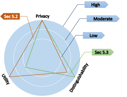
Figure 6. Two examples of the PUD-triangles.

5.1. Privacy Decline

The more times obfuscated training datasets $T_{tr}^{\prime}$ are disclosed, the more likely the raw dataset $T_{tr}$ is exposed by simply calculating the average, if the noises are mutually IID among each sharing. One possible solution could be training over multiple fine-grained subsets which are further sampled from the entire local training dataset $T_{tr}$, and applying the non-IID noise along the training process.

5.2. Training outsourcing on Edge Networks

Model memorization attacks (MLMRTM2017, ) can be exploited in a corrupted training outsourcing task on edge networks. Edge devices with relatively constrained capabilities would have to outsource the training task to the clouds or upper edges by sharing the training dataset. A malicious cloud-based service provider, as the outsourcee, may disclose the raw training dataset $T_{tr}$ to its conspirators by encoding them into the model parameters. Thus, improving the Privacy by the dataset owners (i.e., training outsourcers) obfuscating the dataset before outsourcing them into the machine learning services, as suggested in (noisy-dataset, ). Our experiment results reveal that the model prediction accuracy upon the testing dataset $T_{e}$ is considered acceptable at over 80% on simple tasks with all samples being obfuscated; see Figs. 3(a) and 3(b).

5.3. Proof-of-Learning in FL

The PUD-triangle is particularly useful in a scenario where the model ownership and the proof of “works” for training are both crucial, e.g., the defenses against the model stealing attacks in FL (9519402, ). Stealing others’ models and faking the ownership can be misleading to those who wish to ensure the necessary training overhead. By launching this attack, a malicious edge device with relatively powerful capability can cheat the whole edge network in regards to the amount of “works” that it has done, and steal the rewards. PoL was proposed as a defense strategy against the model stealing attack (9519402, ), which requires the verifiers to replay part of the gradient descent and compare the resultant weights in terms of F-norm $\mathcal{D}$ based on the training dataset $T_{tr}$ shared by the prover (i.e., the owner of the dataset)j; see details in Fig. 7.

Edge devices implementing PoL in FL tasks have to share the training dataset $T_{tr}$, which is contrary to the original design intent of FL to preserve the privacy of $T_{tr}$. Adding random noises to obfuscate $T_{tr}$ helps preserve privacy. However, this concept comes across two possible issues:

• Excessive noise added to $T_{tr}^{i}$ causes a hard differentiation between its obfuscated version $T_{tr}^{i^{\prime}}$ and an arbitrary obfuscated dataset $T_{tr}^{j^{\prime}}$. This is known as the strong disguisability of fakes. By sharing a different dataset, a malicious “prover” can invalidate the PoL.

• Too good utility for an obfuscated dataset $T_{tr}^{\prime}$ can anyhow enrich verifiers’ local datasets. Those who abuse the PoL by raising PoL challenges against as many models as possible can easily outperform those who are challenged due to the unbalanced size of the local training dataset under a non-IID setting.

We propose to settle at a balanced stable point where spoofing the dataset and abusing the PoL to enrich local resources can be prevented, i.e., maximizing Distinguishability and minimizing the Utility, while featuring a high level of Privacy. Figs. 1, 3, 4(c) and 4(d) show the feasibility of meeting the above requirement. Adding a certain level of noise to obfuscate the naked recognition can be achieved (Fig. 1, high Privacy), while sharing others the obfuscated dataset during the PoL process should not retain the dataset utility (Fig. 3, low Utility). Otherwise, malicious attackers in FL could just raise PoL challenges at will to enrich their data resources in a non-IID competition. At the same time, the noise level should not be excessive (Figs. 4(c) and 4(d), high Distinguishability), or it causes a hard differentiation between an obfuscated dataset and an arbitrary dataset. This indicates that a PoL prover could send PoL verifiers a different dataset and pretend to have the correct dataset. As a result, PoL is invalidated by verifiers having to compare the F-norm between the claimed model and the replayed model based on a different dataset. This has been adopted in emerging FL frameworks (yu2023ironforge, ).

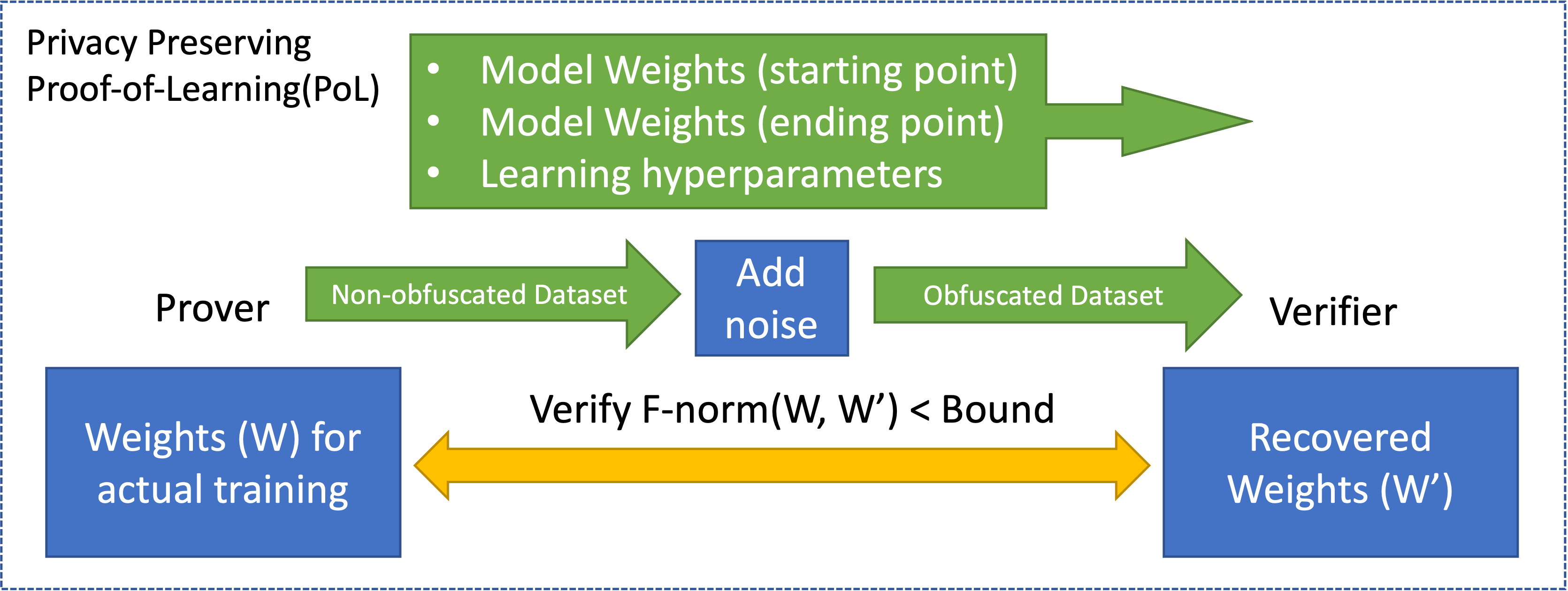
Figure 7. The workflow of Privacy-Preserving PoL.

6. Conclusion

We conducted comprehensive experiments to investigate how obfuscating a training dataset by adding random noises would affect the resultant model in terms of model prediction accuracy, model distance, data utility, data privacy, etc. Experimental results over both the MNIST and CIFAR-10 datasets revealed that, if a balanced point among all the considered metrics is satisfied, broad application prospects on real-world applications will become realistic, including training outsourcing on edge computing and guarding against attacks in FL among edge devices.

References

- [1] He Li, Kaoru Ota, and Mianxiong Dong. Learning iot in edge: Deep learning for the internet of things with edge computing. IEEE Network, 32(1):96–101, 2018.
- [2] Jiasi Chen and Xukan Ran. Deep learning with edge computing: A review. Proceedings of the IEEE, 107(8):1655–1674, 2019.
- [3] Martin Abadi, Andy Chu, Ian Goodfellow, H. Brendan McMahan, Ilya Mironov, Kunal Talwar, and Li Zhang. Deep learning with differential privacy. In Proceedings of the 2016 ACM SIGSAC Conference on Computer and Communications Security, CCS ’16, page 308–318, New York, NY, USA, 2016. Association for Computing Machinery.
- [4] Reza Shokri and Vitaly Shmatikov. Privacy-preserving deep learning. In Proceedings of the 22nd ACM SIGSAC Conference on Computer and Communications Security, CCS ’15, page 1310–1321, New York, NY, USA, 2015. Association for Computing Machinery.
- [5] Ehsan Hesamifard, Hassan Takabi, Mehdi Ghasemi, and Rebecca N Wright. Privacy-preserving machine learning as a service. Proceedings on Privacy Enhancing Technologies, 2018(3):123–142, 2018.
- [6] Olga Ohrimenko, Felix Schuster, Cedric Fournet, Aastha Mehta, Sebastian Nowozin, Kapil Vaswani, and Manuel Costa. Oblivious Multi-Party machine learning on trusted processors. In 25th USENIX Security Symposium (USENIX Security 16), pages 619–636, Austin, TX, August 2016. USENIX Association.
- [7] Raphael Bost, Raluca Ada Popa, Stephen Tu, and Shafi Goldwasser. Machine learning classification over encrypted data. Cryptology ePrint Archive, Paper 2014/331, 2014. https://eprint.iacr.org/2014/331.
- [8] Abbas Acar, Hidayet Aksu, A. Selcuk Uluagac, and Mauro Conti. A survey on homomorphic encryption schemes: Theory and implementation. ACM Computing Surveys, 51(4), jul 2018.
- [9] Tianwei Zhang, Zecheng He, and Ruby B. Lee. Privacy-preserving machine learning through data obfuscation. CoRR, abs/1807.01860, 2018.
- [10] Jiale Zhang, Bing Chen, Yanchao Zhao, Xiang Cheng, and Feng Hu. Data security and privacy-preserving in edge computing paradigm: Survey and open issues. IEEE Access, 6:18209–18237, 2018.
- [11] Hengrui Jia, Mohammad Yaghini, Christopher A. Choquette-Choo, Natalie Dullerud, Anvith Thudi, Varun Chandrasekaran, and Nicolas Papernot. Proof-of-learning: Definitions and practice. In 2021 IEEE Symposium on Security and Privacy (SP), pages 1039–1056, 2021.
- [12] Peva Blanchard, El Mahdi El Mhamdi, Rachid Guerraoui, and Julien Stainer. Machine learning with adversaries: Byzantine tolerant gradient descent. In I. Guyon, U. Von Luxburg, S. Bengio, H. Wallach, R. Fergus, S. Vishwanathan, and R. Garnett, editors, Advances in Neural Information Processing Systems, volume 30. Curran Associates, Inc., 2017.
- [13] Y. Lecun, L. Bottou, Y. Bengio, and P. Haffner. Gradient-based learning applied to document recognition. Proceedings of the IEEE, 86(11):2278–2324, 1998.
- [14] Alex Krizhevsky, Geoffrey Hinton, et al. Learning multiple layers of features from tiny images, 2009.
- [15] Yunlong Lu, Xiaohong Huang, Yueyue Dai, Sabita Maharjan, and Yan Zhang. Differentially private asynchronous federated learning for mobile edge computing in urban informatics. IEEE Transactions on Industrial Informatics, 16(3):2134–2143, 2020.
- [16] Qinbin Li, Yiqun Diao, Quan Chen, and Bingsheng He. Federated learning on non-iid data silos: An experimental study. arXiv preprint arXiv:2102.02079, 2021.
- [17] Congzheng Song, Thomas Ristenpart, and Vitaly Shmatikov. Machine learning models that remember too much. In Proceedings of the 2017 ACM SIGSAC Conference on Computer and Communications Security, CCS ’17, page 587–601, New York, NY, USA, 2017. Association for Computing Machinery.
- [18] Guangsheng Yu, Xu Wang, Caijun Sun, Qin Wang, Ping Yu, Wei Ni, Ren Ping Liu, and Xiwei Xu. Ironforge: An open, secure, fair, decentralized federated learning, 2023.