Do financial regulators act in the public’s interest? A Bayesian latent class estimation framework for assessing regulatory responses to banking crises

Abstract

When banks fail amidst financial crises, the public criticizes regulators for bailing out or liquidating specific banks, especially the ones that gain attention due to their size or dominance. A comprehensive assessment of regulators, however, requires examining all their decisions, and not just specific ones, against the regulator’s dual objective of preserving financial stability while discouraging moral hazard. In this article, we develop a Bayesian latent class estimation framework to assess regulators on these competing objectives and evaluate their decisions against resolution rules recommended by theoretical studies of bank behavior designed to contain moral hazard incentives. The proposed estimation framework addresses the unobserved heterogeneity underlying regulator’s decisions in resolving failed banks and provides a disciplined statistical approach for inferring if they acted in the public interest. Our results reveal that during the crises of 1980’s, the U.S. banking regulator’s resolution decisions were consistent with recommended decision rules, while the U.S. savings and loans (S&L) regulator, which ultimately faced insolvency in 1989 at a cost of $132 billion to the taxpayer, had deviated from such recommendations. Timely interventions based on this evaluation could have redressed the S&L regulator’s decision structure and prevented losses to taxpayers.

Keywords: Bank failures, Federal Deposit Insurance Corporation (FDIC), Federal Savings and Loans Insurance Corporation (FSLIC), Bayesian inference, collapsed Gibbs sampler, Latent class models.

1 Introduction

During financial crises when a large number of banks fail, actions of financial regulators receive substantial public scrutiny. The global financial crisis of 2008 is one such recent example that led to widespread bank failures, reviving debate over how financial regulators might preserve immediate financial stability while also safeguarding against future moral hazard. During a financial crisis, regulators determine and administer the bailout, sale or liquidation of failed banks. Regulators bail out banks when they place greater emphasis on preserving financial stability and liquidate institutions when they are more attentive to the curtailment of moral hazard incentives. Critical assessments of these actions are essential to ensuring regulators balance the competing concerns in a manner that serves the public interest. However, the public typically criticizes specific regulatory decisions instead of evaluating how closely their overall decision framework serves the public interest. Individuals disfavor bailouts because they represent transfers from taxpayers to shareholders. The public also criticizes bank liquidations because they are costly for depositors and loan customers (Isaac, 2010). How can the public and their elected representatives comprehensively assess the actions of regulators against their competing objectives of preserving financial stability and restraining moral hazard?

Theoretical studies of regulator and bank behavior develop decision rules that resolve the trade-off between the two objectives in a manner that maximizes the value of output generated by the banking sector, and thereby provide a benchmark for evaluating such agencies. Broadly, these studies recommend state-dependent decision rules that vary in response to economic and industry-wide conditions that accompanied bank failures (see for example Cordella and Yeyati (2003); Acharya and Yorulmazer (2008); DeYoung et al. (2013) and the references therein). For instance, theoretical models recommend that regulators adopt distinct decision rules for handling banks that failed in the midst of economic distress, and those that failed in normal economic conditions. However, data on bank resolutions do not contain details on the extent to which bank-specific and broader economic conditions were considered in each decision. Furthermore, even though distress in the economy and in the banking industry are observable through measures such as unemployment rate, and growth in output, it is not immediately clear (1) what threshold regulators may have used to distinguish between periods of distress and normalcy, and (2) what aspects of a failed bank’s overall health ultimately inform the regulator’s resolution decision.

In this paper, we develop a Bayesian latent class estimation framework to compare regulators’ decisions against theoretical decision rules that foster financial stability while restraining moral hazard. Theoretical benchmarks recommend applying distinct decision rules that vary by economic and industry conditions, but the thresholds used by regulators to categorize banks into distinct decision rules are unobservable. For instance, when one bank failed in Kansas, and another in Kentucky in 1988 where unemployment rates were 5% and 8.5% respectively, it is not apparent whether regulators considered only one, both or neither banks to have failed amid high distress. The latent class model developed in this paper incorporates such uncertainty by assigning banks into distinct decision rules, or classes with probability, rather than certainty. The proposed model consists of a hierarchical structure (see figure 2) in which the first layer is a probabilistic class-membership model that assigns failed banks to classes that correspond to the two distinct states of nature, such as high or low underlying economic distress. Conditional on class membership, the second layer specifies the relationships between the resolution type, namely assistance, sale or liquidation of failed banks, and bank-specific covariates, such as size and asset quality. These relationships are homogeneous within and heterogeneous across the latent classes when the classes are statistically different from each other. Our approach serves as a classification algorithm that determines whether regulators assigned distinct decision rules to classes of banks that failed in disparate economic and industry conditions, and to systematically infer if they acted in the public interest.

1.1 Regulators of the U.S. banking sector, their resolution methods and the crises of 1980’s

In this article we assess regulators from two sub-sectors of the U.S. banking industry, commercial banks and Savings and Loans (S&L) institutions, during their simultaneous crises of the 1980’s. The Federal Deposit Insurance Corporation (FDIC) serves as the regulatory authority for commercial banks while the Federal Savings and Loans Insurance Corporation (FSLIC) was the counterpart for S&L’s until its failure in 1989. The two regulators are comparable on account of the fundamental similarities across banks and S&L’s in that both institutions offer loans and deposits, undertake maturity transformation, monitor information and offer liquidity and payments services (Freixas and Rochet, 2008).

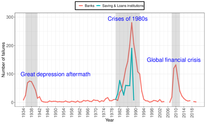
Figure 1: Number of failed banks resolved by the FDIC and number of failed S&L’s resolved by the FSLIC from 1934 to 2020.

During the crises of 1980’s, these two related sectors of the U.S. banking industry, namely commercial banks and S&L’s, witnessed the highest number of failures since the Great Depression as depicted in Figure 1. Notably, the FDIC and FSLIC underwent contrasting trajectories following the crises. While the FDIC survived the crisis, albeit with depleted insurance funds, the FSLIC faced insolvency by the end of the crisis and was closed in 1989 at a cost of $132 billion to the taxpayer (FDIC, 1998).

When banks and S&Ls failed, the FDIC and FSLIC applied one of the following three resolution methods (Walter, 2004):

1. Type I: Open Bank Assistance (OBA) - Under this resolution method, the regulator provides financial assistance to acquirers toward the purchase of a failing bank or grants direct assistance to the failing bank.

2. Type II: Purchase and Assumption (P&A) - Resolutions under this category consist of acquiring a part of the assets and liabilities of a failed bank by a participating institution.

3. Type III: Deposit Payout (PO) - Under this resolution category, the regulator liquidates the failed institution and pays out its insured depositors from the insurance fund.

Each of the three resolution methods described above involve a progressively more severe breakdown of relationships between the bank and its customers (Ashcraft, 2005). For instance while a Type I resolution method ensures continuity of banking relationships, a Type III resolution terminates all such relationships. We compare the decision rules employed by the FDIC and FSLIC in assigning of the three resolution methods to failed institutions during the crises of 1980’s in addition to assessing their decisions against recommended decision rules from theoretical studies. Our results expose specific weaknesses in the FSLIC’s decision structure and the FDIC’s relative strengths that are likely to have contributed to the former’s failure in 1989 and the latter’s continued survival.

The crises of the 1980’s are particularly suitable for comparing the resolution decisions of FDIC and FSLIC against theoretically recommended state-dependent decision rules for several reasons. First, the simultaneous crises in banking and S&L industries in the 1980’s provided a basis to compare the two regulators, and to identify the stronger of the two approaches to resolving failed institutions. Second, bank and S&L failures in this period occurred against the backdrop of shocks in specific sectors, namely, agriculture, real-estate and energy that resulted in regional crises (FDIC, 1998). For instance, the major sectoral crises that occurred during this period were the recessions following the collapse of energy prices in Texas, Louisiana and Oklahoma, the agricultural recession in Kansas, Iowa and Nebraska and the real-estate-led downturns in California, the Southwest and the Northeast (FDIC, 1997). Third, banks were subject to varying levels of branching restrictions and operated either within state borders or across states that had entered into reciprocal arrangements (Kroszner and Strahan, 1999). Specifically, this period predates the elimination of the interstate branching restrictions mandated by the 1994 Riegle-Neal Interstate Banking and Branching Efficiency Act (Medley, 2013). Thus, the combination of sectoral crises that were regionally contained and branching restrictions that limited the geographic scope of banking markets entailed that certain bank failures occurred amid economic and financial distress, and others, in relatively normal economic conditions. This provided an ideal setting for the two regulators towards implementing the theoretically recommended state-dependent decision rules for resolving failed banks during this crisis.

1.2 Recommended decision rules from theoretical studies and testable hypotheses

In this section we first discuss the decision rules that are recommended by the branches of theoretical literature for the resolution of failed banks under two state-dependent scenarios - economic distress and banking industry distress. Thereafter, we identify the specific testable hypotheses for each of these scenarios as wells as the hypothesis to infer the impact of political influence on regulators’ resolution decisions.
 
Economic distress and recommended decision rule for bank resolutions - Cordella and Yeyati (2003) determined a resolution strategy, or a decision rule, in which the regulator provides bailouts to banks if their failure occurred under macroeconomic distress, when bank failures are less likely to have arisen due to their unsound portfolio decisions and more likely to have arisen due to exogenous factors. Correspondingly, in the event of bank failures under normal economic conditions, their theoretical model recommended liquidating such banks.
 
Hypothesis $H_{1}$: The testable hypothesis is that the FDIC and FSLIC applied different decision rules for banks that failed in normal economic conditions and those that failed amid macroeconomic distress. Conditional on the presence of two distinct rules, the subsequent statistical inference centers on testing the hypothesis that the probability of receiving a Type I resolution was higher for banks that failed amid high economic distress relative to those that failed amid low distress.
 
Banking industry distress and recommended decision rule for bank resolutions - Acharya and Yorulmazer (2007, 2008) propose resolution strategies for the “too-many-to-fail” problem or, equivalently, the simultaneous failure of many banks. Their recommended decision rule consisted of facilitating acquisitions of failed banks when such failures were small in number but providing bailouts and financial assistance when there were a large number of failures.
 
Hypothesis $H_{2}$: The first testable hypothesis is that regulators applied distinct rules in the presence and absence of banking industry distress. Second, the decision rule employed in the presence of banking industry distress designated a higher proportion of resolutions as Type I compared to the rule applied in its absence.
 
Political influence on regulators’ decision rule for bank resolutions - Several empirical studies (Igan et al., 2012; Duchin and Sosyura, 2012) have revealed the evidence of political and lobbying influence on regulators’ decisions for bank resolutions. For instance, DeYoung et al. (2013) find that when a regulator experiences political pressure to place greater emphasis on maintaining current liquidity, they will provide more bailouts than when the regulator prioritizes the prevention of future moral hazard.
 
Hypothesis $H_{3}$: The primary hypothesis is that the presence of political influence induces a separate decision rule that is distinct from the rule applied in its absence. Subsequently, inferences center on whether the decision rule utilized under political influence resulted in a higher probability of receiving a Type I resolution relative to the rule applied in the absence of political influence.

1.3 Our contributions and connections to existing works

We consider the three hypotheses from Section 1.2 and test for the presence of state-dependent resolution strategies, either recommended by theory or arising from political interference, in the decision rules employed by the FDIC and FSLIC to resolve failed banks and S&Ls during the crises of 1980’s. Our findings reveal that regular assessments of financial regulators by lawmakers and the public can uncover gaps between observed and recommended resolution rules and provide guidelines for corrective actions. For instance, timely assessments of the FSLIC could have revealed that the agency had provided excessive assistance to institutions that failed amid relatively normal economic conditions and to institutions that received political support (Section 5). Interventions based on these assessments could have potentially prevented both, the failure of FSLIC in 1989 and the ensuing costs to the taxpayer. Conversely, the decision structure of the FDIC identified in this paper (Section 4) provides a road-map for newer resolution agencies that face widespread failures from systemic shocks. The ensuing discussion summarizes our main contributions.

1. This paper contributes to the empirical literature examining bank resolution decisions in two ways. First, we statistically evaluate how regulators’ decisions align with recommended decision rules from alternative theoretical models, as well as the extent to which political economy factors interfere with those recommended decisions. Second, and to the best of our knowledge, this is the first article to compare between the decision rules of the FDIC and FSLIC during the simultaneous crises in the banking and S&L industries during the 1980’s.

2. To evaluate the three hypotheses in Section 1.2, we develop a new methodology for assessing regulators in the form of a Bayesian latent class estimation framework for ordered outcomes. The proposed framework detects unobserved heterogeneity in regulators’ resolution decisions based on underlying economic and political conditions. For estimating this model and conducting inference, we design a novel collapsed Gibbs sampler algorithm that provides a technique for efficient sampling from the posterior distribution relative to standard approaches by reducing the autocorrelations across successive draws. Our method provides a statistical framework to compare parameters across the latent classes, and additionally allows for inferences on all estimated quantities of interest, including marginal effects and the probability of class membership.

3. We consider hypothesis $H_{1}$ and evaluate whether the FDIC and FSLIC provided bailouts to banks or S&L’s that failed amid macroeconomic distress and withheld such assistance for failures in normal economic conditions. Our results reveal that the FSLIC deviated from and the FDIC adhered to this theoretically recommended rule. Specifically, banks that failed amid high economic distress received financial assistance, or bailouts from the FDIC with an average probability of 25% compared to 3% for banks that failed amid low distress. The FSLIC, on the contrary, assigned Type I assistance with probabilities 68% and 70% to the two groups of S&L institutions that did not statistically differ across measures of macroeconomic distress.

4. We examine hypothesis $H_{2}$ on whether the two regulatory agencies experienced a too-many-to-fail problem and responded to it in the form of a greater reliance on bailouts and financial assistance to acquiring institutions. Our results show that the FDIC’s decision rules aligned with the theoretical rules as the agency provided Type I assistance with a probability of 27% for failures amid economic and banking industry distress and a statistically lower probability of 4% for failures amid low levels of such distress. The FSLIC assigned Type I assistance with probabilities of 76% and 70% among groups of institutions that did not statistically differ by industry and economic distress.

5. We evaluate hypothesis $H_{3}$ and assess the extent to which political pressures influenced the resolution decisions of the two agencies. Whereas the previous two hypotheses examined the extent to which regulators followed recommended theoretical rules, this assessment examines potential institutional weaknesses. We find that political support for the banking industry played a limited role in the FDIC’s decisions, but a more salient role in the FSLIC’s decisions. Notably, the FSLIC assigned assistance to S&L’s that likely received a higher degree of political support and failed amid lower economic distress at a statistically higher probability of 92% relative to 59% for S&L’s that failed amid low political support and in a climate of higher economic distress.

A rich literature examined the financial costs incurred by the FDIC (Bennett and Unal, 2014; Balla et al., 2015) and the weaknesses of the FSLIC (Kane, 1989; Akerlof et al., 1993; Romer and Weingast, 1991; White, 1991). The empirical results in this paper align with the sources of weaknesses in the FSLIC’s decision structure discussed in previous literature. However, prior literature has not formally assessed both agencies against resolution rules recommended by theoretical models. Relatedly, the decision rules of the two agencies have not been compared with each other. Our paper addresses both these gaps in the literature.

Greene and Hensher (2010) developed a classical method to estimate latent class models with ordered outcomes by way of an Expectation-Maximization algorithm. Heckman and Singer (1984) proposed latent class models as a nonparametric alternative to random coefficients models in addressing unobserved heterogeneity without the problems of “over-parameterization” and excessive sensitivity to distributional assumptions associated with the latter method. Latent class models have since been developed for a range of outcomes including multinomial (Greene and Hensher, 2003; Burda et al., 2008), count (Wang et al., 1998; Wedel et al., 1993; Deb and Trivedi, 1997; Nagin and Land, 1993) and ordered (Greene et al., 2014) responses. These works apply latent class models to study heterogeneity in fields ranging across healthcare, marketing and transportation. Here we provide a new interpretation of latent class models as a tool to assess banking regulators and develop a framework for evaluating regulators in the event of future crises.

1.4 Organization

The rest of the article is organized as follows. In Section 2 we discuss the data used in this article. Section 3 presents the proposed Bayesian latent class estimation framework for evaluating the regulatory decision rules for resolving bank failures against recommended decision rules from theoretical studies. In Section 4 we discuss the results of our analysis pertaining to the FDIC’s resolution decisions while Section 5 is dedicated to analyzing the FSLIC’s resolution decisions. The article concludes with a discussion in Section 6. Additional technical details, numerical results and background information are relegated to the supplementary materials.

2 Data

We examine bank resolutions by the FDIC between 1984 and 1992 and S&L resolutions by the FSLIC from 1984 until the agency’s closure in 1989. The period between 1984 and 1992 is particularly suited to evaluate the decisions of the FDIC since the agency was subject to restrictions in applying Type I resolutions before 1982 and after $1993$ . The FSLIC, on the contrary, retained this authority from the start of the sample period until its closure in 1989.

The data used in this paper includes variables that can be broadly divided into seven categories that we describe below.

1. Data on resolution methods - the data on resolution methods applied to failed banks and S&L’s are obtained from the Historical Statistics on Banking (HSoB) maintained by the FDIC. The sample consists of 1385 banks, of which there are 118, 1175 and 92 institutions resolved under resolution types I, II and III respectively. There are 389 S&L institutions in the sample of which 270, 104 and 15 institutions underwent resolution methods I, II and III respectively.

2. Bank and S&L-level characteristics - failed banks from the HSoB are matched with call report data from the Federal Reserve Bank of Chicago to obtain information from the financial statements of each institution. We aggregate the call reports by certificate number, which the FDIC uniquely assigns to each head office of depository institutions, and use this identifier to merge the two datasets. To allow for the duration of 90 to 100 days (FDIC, 1998) between the FDIC receiving notification of an institution that is in danger of failing and determining the resolution method, call reports from two quarters prior to the date of failure are used in the study.

   The failed S&L institutions in the sample are matched with Thrift Financial Reports as of six months prior to failure from the Research Information System (RIS) of the FDIC. The data on S&L institutions is less extensive than the corresponding bank-level data due to differences in the reporting requirements for banks and S&L’s. Specifically, data on Agricultural loans, Nonperforming loans and Core Deposits are not available for S&L institutions for the period under study.

3. Insurer characteristic - we obtain the year-end data on outstanding balances on the deposit insurance fund of the FDIC from annual reports from the agency’s website. The balances on the FSLIC’s insurance fund are obtained from FDIC (1997). These balances remain constant across banks and S&L’s, and vary by year. We use this information to calculate the amount of deposit insurance fund as a percentage of total deposit for both FDIC and FSLIC. This characteristic measures the extent of insurance funds available to the two agencies relative to the maximum value of their potential insurance payouts.

4. State characteristics - our data hold several dimensions of information pertaining to the states in which the banks and S&L’s operated. Specifically, the data on quarterly housing starts at the state level have been obtained from IHS Global Insight, the data on annual unemployment at the state level were obtained from the Iowa Community Indicators Program of Iowa State University and the information on branching deregulation laws was collated using the table in Strahan et al. (2003).

5. County characteristics - the data pertaining to county economic characteristics in which the banks and S&L’s operated have been collated from the Bureau of Economic Analysis. These characteristics consist of per capita growth in gross domestic product (GDP) and the share of employment in each sector, which measure the economic output of each county and the importance of each sector to the county’s economy respectively.

6. County-level characteristics of bank distress -county-level statistics on the banking industry are obtained by aggregating bank-level data from the Research Information System (RIS) of the FDIC, which is available starting from 1984.

7. State-level political economy characteristics - Congressional voting data were obtained from the website of GovTrack (https://www.govtrack.us) and converted into state-level percentages of representatives who voted in favor of each bill evaluated in this study. The description of these bills is available in Section A of the supplement.

Table 3 in Section A of the supplement provides a description of the variables available under each of these seven categories. Tables 4 and 5 in Section A provide summary statistics of the data across these seven categories for FDIC and FSLIC resolution decisions, respectively. In these tables, the Texas Ratio for a bank is defined as,

$$\mbox{Texas Ratio}=\frac{\mbox{Non-performing Assets}}{\mbox{Tangible Equity + Loan Loss Reserves}}.$$ (1)

The Texas-Ratio is a measure of distress as it identifies institutions whose capital would be insufficient to absorb losses that could emanate from nonperforming assets.

3 Bayesian latent class estimation framework

In this section, we propose a Bayesian latent class estimation framework for ordinal outcomes to represent the decision rules of FDIC and FSLIC in resolving failed banks and to evaluate these decision rules against recommended rules from theoretical studies.

3.1 Ordering of resolution decisions

We model the primary outcome of interest, the resolution decision of the FDIC and FSLIC, as an ordered variable by specifying the three resolution methods of Section 1.1 as ordered categories. Previous studies have shown that these resolution methods resulted in progressively more severe effects on economic outcomes (Ashcraft, 2005) and on the level of liquidity (DeYoung et al., 2013). In particular, Ashcraft (2005) points out that each of the three resolution categories entail an increasingly severe breakdown of relationships between the bank and its customers. The provision of Type I assistance allows a bank to continue functioning in its present form. A Type II acquisition or purchase results in certain loan and deposit relationships continuing within the acquiring bank’s books. A Type III liquidation and deposit payout results in the termination of all banking relationships. The specification of resolution methods as an ordered outcome variable also allows for a decision structure in which the regulators order banks by their franchise value and assign Type I resolutions to the most valuable and Type III resolutions to the least valuable banks. Such an ordering of banks and S&Ls by franchise value is consistent with a cost-minimization objective, which was relevant to both FDIC and FSLIC since they were required to preserve their insurance funds by controlling their costs of resolution (FDIC, 2007).

In the following discussion, bank $i$ refers to a representative bank or S&L without loss of generality. Let $y_{i}$ be the resolution method applied on bank $i$ where $y_{i}$ takes values $1,2$ and $3$ to denote resolution types I, II and III respectively.

3.2 Latent class model for ordinal outcomes

We use a latent class model to represent state-dependent rules in the two regulators’ decision structure. Figure 2 depicts the structure of the latent class model. The class indicator $s_{i}$ is introduced into the model to denote assignment of bank $i$ into one of the two classes. Within each latent class, the regulator applies a class-specific decision rule on the failed bank $i$ to assign it one of the three available resolution methods.

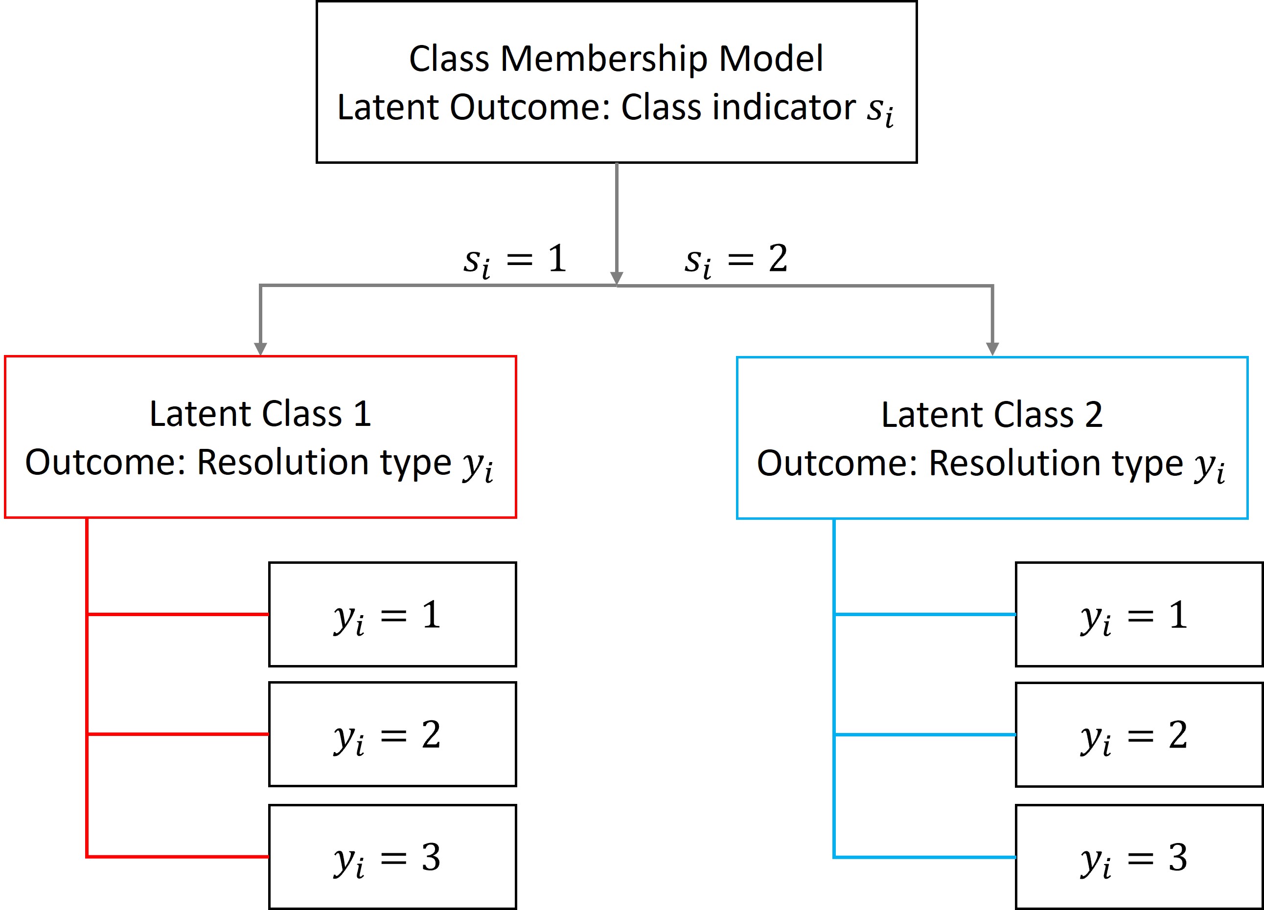
Figure 2: Structure and components of the latent class model for bank resolutions. Here index $i$ refers to a representative bank or S&L $i$.

The distinguishing feature of the latent class model is that classes are determined with probability and not deterministically. This feature is relevant to the current problem since the true assignment of banks into distinct classes by regulators is not observable as the data record the final decision made by the regulators but not the rationale that motivated each decision. Specifically, $y_{i}$ is observed but $s_{i}$ is not. As a result, the probabilistic assignment of banks into classes addresses the researcher’s uncertainty on class assignments by the regulatory agencies.

Relatedly, the recommended decision rules from theoretical models described in Section 1.2 consisted of state-dependent rules, which entailed heterogeneity in relationships between the outcome and covariates across sub-groups of banks that failed in different states of nature. Moreover, each distinct decision rule recommended by theoretical studies represents a distinct latent class in our hierarchical model. Therefore, the latent class structure permits a direct comparison between theoretical decision rules and the observed decisions of the FDIC and FSLIC.

3.3 Random utility framework

The random utility representation of this model is based on the framework developed by Marschak (1974). We model the regulator’s problem of assigning bank $i$ to one of the two latent classes as a binary discrete choice problem with a latent outcome $s_{i}$. To apply the random utility representation to this discrete choice problem, we introduce a continuous latent variable $l_{i}$, which represents the difference in utilities or value to the regulator from assigning bank $i$ to latent class 2 relative to latent class 1. We express $l_{i}$ as,

$$l_{i}=\bm{w}_{i}^{\prime}\bm{\alpha}+\nu_{i},$$ (2)

where $\bm{w}_{i}$ is a $p-$dimensional vector of covariates, $\bm{\alpha}$ are parameters and $\nu_{i}$ is the error term. Finally, the relationship between the discrete variable $s_{i}$ and the continuous variable $l_{i}$ is expressed via the following threshold crossing framework,

$$s_{i}=\begin{cases}1&\text{if}\ l_{i}\leq 0\\ 2&\text{otherwise}\end{cases}.$$

The covariates $\bm{w}_{i}$ in Equation (2) are determined by the three hypotheses of interest described in Section 1.2. For instance, in testing hypothesis $H_{1}$, the covariates consist of economic indicators pertaining to the state and the county in which bank $i$ operates, for hypothesis $H_{2}$, they contain measures of the banking industry’s health in the county in which bank $i$ operates and for hypothesis $H_{3}$, the covariates include the percentage of Congressional representatives in banks $i$’s state who voted for various bills that were favorable to the banking industry.

Within latent class $s_{i}$, the regulator’s utility function $z_{i,s_{i}}$ determines the final resolution method applied on bank $i$ where,

$$z_{i,s_{i}}=\begin{cases}\bm{x}_{i}^{\prime}\bm{\beta}_{1}+\epsilon_{i,1},&\text{if}~{}s_{i}=1\\ \bm{x}_{i}^{\prime}\bm{\beta}_{2}+\epsilon_{i,2},&\text{if}~{}s_{i}=2\end{cases}.$$ (3)

Here $z_{i,s_{i}}$ is the utility that the regulator derives from preserving bank $i$’s franchise value as discussed in Section 3.1. The $q-$dimensional covariate vector $\bm{x}_{i}$ consists of bank $i$’s characteristics that are representative of its financial health and importance, salient among which are its size, the quality of its assets and composition of risky asset classes. Note that in Equation (3), $\bm{x}_{i}^{\prime}\bm{\beta}_{s}$ and $\epsilon_{i,s}$ represent the observable and unobservable components of utility respectively (Train, 2009) for $s\in\{1,2\}$. The relationship between the observed outcome $y_{i}$ and the latent utility $z_{i,s_{i}}$ is represented using the following threshold-crossing framework,

$$y_{i}=\begin{cases}3:\hskip 5.0pt\text{Type III},&\text{if}\ -\infty<z_{i,s_{i}}\leq\gamma_{1,s_{i}}\\ 2:\hskip 5.0pt\text{Type II},&\text{if}\ \gamma_{1,s_{i}}<z_{i,s_{i}}\leq\gamma_{2,s_{i}}\\ 1:\hskip 5.0pt\text{Type I},&\text{if}\ \gamma_{2,s_{i}}<z_{i,s_{i}}\leq\infty\\ \end{cases}.$$ (4)

The regulator selects a resolution method that preserves more of the bank’s franchise value as $z_{i,s_{i}}$ crosses a progressively larger threshold. When $z_{i,s_{i}}$ is below the lowest threshold, $\gamma_{1,s_{i}}$, bank $i$ loses all its franchise value as the regulator’s utility level corresponds to liquidation under a Type III resolution.

3.4 Likelihood function

The likelihood contribution $P_{ij}$ of bank $i$ receiving resolution type $j=1,2,3$ is the sum of the likelihood contribution based on each latent class weighted by the marginal probability of belonging to each of the two latent classes,

$$P_{ij}=\sum_{s=1}^{2}P_{ij|s}Q_{is},$$ (5)

where $P_{ij|s}$ is the probability of $y_{i}$ taking a particular value $j$ conditional on belonging to class $s_{i}=s\in\{1,2\}$ and $Q_{is}$ is the corresponding probability of bank $i$ belonging to class $s$. With $\nu_{i}$ in Equation (2) distributed independently as $\mathcal{N}(0,1)$, we obtain the following binary probit representation of the class membership model,

$$Q_{is}={\Phi(\bm{w}_{i}^{\prime}\bm{\alpha})}^{s^{\prime}}\Bigl{\{}1-\Phi(\bm{w}_{i}^{\prime}\bm{\alpha})\Bigr{\}}^{1-s^{\prime}},s^{\prime}=s-1,\hskip 10.0pts\in\{1,2\}.$$ (6)

On specifying a $\mathcal{N}(0,\sigma^{2}_{s})$ distribution for the unobserved component $\epsilon_{i,s}$ in Equation (3), the probability of $y_{i}$ taking a particular value $j$ conditional on class $s_{i}=s\in\{1,2\}$ from Equation (4) is,

$$P_{ij|s}=\begin{cases}\Phi\Big{(}\dfrac{\gamma_{1,s}-\bm{x}_{i}^{\prime}\bm{\beta}_{s}}{\sigma_{s}}\Big{)},~{}&\text{if}~{}j=3\\ \Phi\Big{(}\dfrac{\gamma_{2,s}-\bm{x}_{i}^{\prime}\bm{\beta}_{s}}{\sigma_{s}}\Big{)}-\Phi\Big{(}\dfrac{\gamma_{1,s}-\bm{x}_{i}^{\prime}\bm{\beta}_{s}}{\sigma_{s}}\Big{)},~{}&\text{if}~{}j=2\\ 1-\Phi\Big{(}\dfrac{\gamma_{2,s}-\bm{x}_{i}^{\prime}\bm{\beta}_{s}}{\sigma_{s}}\Big{)},~{}&\text{if}~{}j=1\end{cases}.$$ (7)

In estimating the ordinal outcome model $P_{ij|s}$ conditional on class membership $s$, we use the identification scheme in which the cut-points $\gamma_{1,1}$ and $\gamma_{1,2}$ are restricted to 0 and the cut-points $\gamma_{2,1}$ and $\gamma_{2,2}$ are restricted to 1 (Jeliazkov and Rahman, 2012).This identification restriction eliminates the need for estimating cut-points and allows the scale parameter $\sigma_{s}$ to be estimated as a free parameter in each latent class. As discussed in Jeliazkov and Rahman (2012) and Greene and Hensher (2010), identification restrictions are required in estimating ordinal models as neither the scale nor the location of the latent variable $z_{i}$ is identified in this category of models.

Denote $\bm{\Theta}=\{\bm{\beta}_{1},\bm{\beta}_{2},\sigma_{1}^{2},\sigma_{2}^{2},\bm{\alpha}\}$. The likelihood function is obtained as,

$$\mathcal{L}(\bm{\Theta})=\prod_{i=1}^{n}\Bigl{\{}\prod_{j=1}^{3}\Big{(}P_{ij}\Big{)}^{\mathbb{I}\{y_{i}=j\}}\Bigr{\}},$$

where $P_{ij}$ and its components are as defined in equations (5), (6), (7), and $\mathbb{I}\{y_{i}=j\}=1$ if $y_{i}=j$ and $0$ otherwise.

3.5 Augmented posterior

The augmented posterior for the parameters and latent variables in this model is obtained by augmenting the likelihood with the latent variables $\bm{z}=(z_{1,s_{1}},\ldots,z_{n,s_{n}})$ and $\bm{u}=(s_{1},\ldots,s_{n})$ using the method of Albert and Chib (1993). Denote

$$\mathcal{B}_{i}=\begin{cases}(-\infty,0],~{}&\text{if}~{}y_{i}=3\\ (0,1],~{}&\text{if}~{}y_{i}=2\\ (1,\infty),~{}&\text{if}~{}y_{i}=1\\ \end{cases}.$$

Using equations (2)-(7), the resulting expression for the augmented posterior is,

$$f(\bm{\Theta},\bm{z},\bm{u}|\bm{y})\propto\Big{[}\prod_{i=1}^{n}\Bigl{\{}\mathbb{I}\{z_{i,1}\in\mathcal{B}_{i}\}f_{\mathcal{N}}(z_{i,1}|\bm{x}_{i}^{\prime}\bm{\beta}_{1},\sigma_{1})Q_{i1}+\mathbb{I}\{z_{i,2}\in\mathcal{B}_{i}\}f_{\mathcal{N}}(z_{i,2}|\bm{x}_{i}^{\prime}\bm{\beta}_{2},\sigma_{2})Q_{i2}\Bigr{\}}\Big{]}h(\bm{\Theta}),$$ (8)

where $\bm{y}=(y_{1},\ldots,y_{n})$, $\mathbb{I}\{z_{i,s}\in\mathcal{B}_{i}\}$ takes the value $1$ if $z_{i,s}\in\mathcal{B}_{i}$ and $0$ otherwise, $f_{\mathcal{N}}(z_{i,s}|\bm{x}_{i}^{\prime}\bm{\beta}_{s},\sigma_{s})$ is the density of a normal distribution with mean $\bm{x}_{i}^{\prime}\bm{\beta}_{s}$ and standard deviation $\sigma_{s}$ for $s\in\{1,2\}$ and $h(\bm{\Theta})$ is the joint probability density function of the prior distribution of the parameters in $\bm{\Theta}$. We assign a $q-$dimensional multivariate normal prior to $\bm{\beta}_{s}$ that has mean $\bm{\beta}_{0,s}$ and covariance $B_{0,s}$, and an Inverse Gamma prior to $\sigma_{s}^{2}$ with shape parameter $v/2$ and scale parameter $d/2$. Finally, we assign a $p-$dimensional multivariate normal prior to $\bm{\alpha}$ with mean $\bm{\alpha}_{0}$ and covariance $A_{0}$. Since the priors are independent, their joint density $h(\bm{\Theta})$ in Equation (8) can be represented as,

$$h(\bm{\Theta})=\Bigl{\{}\prod_{s=1}^{2}f_{\mathcal{N}}(\bm{\beta}_{s}|\bm{\beta}_{0,s},B_{0,s})f_{\mathcal{IG}}\Big{(}\sigma_{s}^{2}\Big{|}\dfrac{v}{2},\dfrac{d}{2}\Big{)}\Bigr{\}}f_{\mathcal{N}}(\bm{\alpha}|\bm{\alpha}_{0},A_{0}),$$

where $f_{\mathcal{IG}}(\sigma_{s}^{2}|v/2,d/2)$ is the density of an Inverse Gamma distribution with shape parameter $v/2$ and scale parameter $d/2$.

3.6 MCMC algorithm

A standard approach to developing an MCMC algorithm results in a Gibbs sampler that draws from the full conditionals of all parameters as well as the two latent variables $\bm{u}$ and $\bm{z}$. In this section we present a Collapsed Gibbs sampler (Liu, 1994) which provides an efficient technique for sampling from the posterior distribution relative to standard sampling approaches by reducing autocorrelations across successive draws. Specifically, in our algorithm, we do not have to draw from the conditionals of $\bm{u}$ as we sample for the parameters of the class membership model, $\bm{\alpha}$, independently of this latent variable. We first present the algorithm for our collapsed Gibbs sampler and then discuss the details underlying each step in the sampler.
 
Algorithm: Collapsed Gibbs Sampler

1. Sample $\bm{\beta}_{s}$ from the distribution $\bm{\beta}_{s}|\bm{z},\bm{u},\sigma^{2}_{s}$ for $s\in\{1,2\}$.

2. Sample $\sigma^{2}_{s}$ from $\sigma^{2}_{s}|\bm{\beta}_{s},\bm{z},\bm{u}$ for $s\in\{1,2\}$.

3. Sample $\bm{\alpha}$ from $\bm{\alpha}|\bm{\beta},\bm{\sigma}^{2},\bm{y}$ where $\bm{\sigma}^{2}=(\sigma^{2}_{1},\sigma^{2}_{2})$ and $\bm{\beta}=(\bm{\beta}_{1},\bm{\beta}_{2})$.

4. Sample $s^{\prime}_{i}$ from $s^{\prime}_{i}|\bm{\alpha},\bm{\beta},\bm{\sigma}^{2},\bm{y}$, where $s_{i}^{\prime}=s_{i}-1$ for $i=1,\ldots,n$.

5. Sample $z_{i,s_{i}}$ from $z_{i,s_{i}}|\bm{\beta},\bm{\sigma}^{2},\bm{y},\bm{u}$ for $i=1,\ldots,n$.

For the following discussion, denote $X$ to be the $n\times q$ matrix with the vector of $q$-dimensional covariates $\bm{x}_{i}^{\prime}$ from Equation (3) in its rows.
 
Sampling coefficients $\bm{\beta}_{s}$ of the ordinal model - The coefficients $\bm{\beta}_{s}$ of the ordinal model are sampled for the two latent classes, i.e., for $s\in\{1,2\}$ from their respective conditional posterior distributions. We have $\bm{\beta}_{s}|\bm{z},\bm{u},\sigma^{2}_{s}\sim\mathcal{N}\bigl{(}\hat{\bm{\beta}}_{s},\hat{B}_{s}\bigr{)}$, where $\hat{B}_{s}=\bigl{(}B_{0,s}^{-1}+X_{s}^{\prime}X_{s}/\sigma_{s}^{2}\bigr{)}^{-1}$ and $\hat{\bm{\beta}}_{s}=\hat{B}_{s}\bigl{(}B_{0,s}^{-1}\bm{\beta}_{0,s}+X_{s}^{\prime}\bm{z}_{s}/\sigma_{s}^{2}\bigr{)}$. Here $X_{s}$ is the $n_{s}\times q$ submatrix of $X$ that includes those rows of $X$ for which $s_{i}=s$ and $n_{s}$ is the number of observations in class $s$ which is updated in every MCMC iteration. Similarly, $\bm{z}_{s}$ denotes the length $n_{s}$ subvector of $\bm{z}$ that includes those elements of $\bm{z}$ for which $s_{i}=s$. In this sampling step, the computations involving $X_{s}$ are efficient as they only require working with matrices of reduced dimension $n_{s}\times q$, without having to preserve the full $n\times q$ matrix $X$.
 
Sampling the variance $\sigma^{2}_{s}$ of the ordinal model - The variances are sampled using the conditionals $\sigma^{2}_{s}|\bm{z},\bm{u},\bm{\beta}_{s}\sim\mathcal{IG}({\sf shape=}~{}\hat{\nu}_{s},{\sf scale=}~{}\hat{d}_{s})$ for $s\in\{1,2\}$, where $\hat{\nu}_{s}=(\nu+n_{s})/2$ and $\hat{d}_{s}=\bigl{\{}d+(\bm{z}_{s}-X_{s}\bm{\beta}_{s})^{\prime}(\bm{z}_{s}-X_{s}\bm{\beta}_{s})\bigr{\}}/2$. Here $X_{s}$ and $\bm{z}_{s}$ are retained from the previous step.
 
Sampling coefficients $\bm{\alpha}$ of the class membership model - The coefficients $\bm{\alpha}$ of the class membership model are sampled from $\bm{\alpha}|\bm{\beta},\bm{\sigma}^{2},\bm{y}$, marginally of $\bm{u}$, by using a Metropolis Hastings (MH) step with a tailored proposal distribution. We use a $p-$dimensional $t$ distribution with location parameter $\hat{\bm{\alpha}}$, covariance matrix $\mathcal{V}$ and degrees of freedom $v$ as the tailored proposal distribution where $\hat{\bm{\alpha}}=\operatorname*{arg\,max}_{\bm{\alpha}}f(\bm{y}|\bm{\alpha},\bm{\beta},\bm{\sigma}^{2})f_{\mathcal{N}}(\bm{\alpha}|\bm{\alpha}_{0},A_{0})$, $\mathcal{V}$ is the inverse of the negative Hessian of $\log\{f(\bm{y}|\bm{\alpha},\bm{\beta},\bm{\sigma}^{2})f_{\mathcal{N}}(\bm{\alpha}|\bm{\alpha}_{0},A_{0})\}$ evaluated at $\hat{\bm{\alpha}}$ and

$$f(\bm{y}|\bm{\alpha},\bm{\beta},\bm{\sigma}^{2})=\prod_{i=1}^{n}\Big{[}\Bigl{\{}1-\Phi(\bm{w}_{i}^{\prime}\bm{\alpha})\Bigr{\}}P_{y_{i}|1}+\Phi(\bm{w}_{i}^{\prime}\bm{\alpha})P_{y_{i}|2}\Big{]},$$

with

$$P_{y_{i}|s}=\begin{cases}\Phi\Big{(}\dfrac{\gamma_{1,s}-\bm{x}_{i}^{\prime}\bm{\beta}_{s}}{\sigma_{s}}\Big{)},~{}&\text{if}~{}y_{i}=3\\ \Phi\Big{(}\dfrac{\gamma_{2,s}-\bm{x}_{i}^{\prime}\bm{\beta}_{s}}{\sigma_{s}}\Big{)}-\Phi\Big{(}\dfrac{\gamma_{1,s}-\bm{x}_{i}^{\prime}\bm{\beta}_{s}}{\sigma_{s}}\Big{)},~{}&\text{if}~{}y_{i}=2\\ 1-\Phi\Big{(}\dfrac{\gamma_{2,s}-\bm{x}_{i}^{\prime}\bm{\beta}_{s}}{\sigma_{s}}\Big{)},~{}&\text{if}~{}y_{i}=1\end{cases},$$ (9)

for $s\in\{1,2\}$. This MH step enhances the efficiency of the overall algorithm by circumventing the need for additional data augmentation through the latent variable $l_{i}$ from Equation (2).

The proposed draw $\bm{\alpha}^{\dagger}$ from this proposal is accepted with probability,

$$\Upsilon_{MH}(\bm{\alpha},\bm{\alpha}^{\dagger})=\min\Bigg{\{}1,\dfrac{f(\bm{\alpha}^{\dagger}|\bm{\beta},\bm{\sigma}^{2},\bm{y})q(\bm{\alpha}|\bm{\beta},\bm{\sigma}^{2},\bm{y})}{f(\bm{\alpha}|\bm{\beta},\bm{\sigma}^{2},\bm{y})q(\bm{\alpha}^{\dagger}|\bm{\beta},\bm{\sigma}^{2},\bm{y})}\Bigg{\}},$$

where $q(\bm{\alpha}|\bm{\beta},\bm{\sigma}^{2},\bm{y})$ is the density of the tailored proposal distribution and the expression $f(\bm{\alpha}|\bm{\beta},\bm{\sigma}^{2},\bm{y})$ in the display above is proportional to the product of $f(\bm{y}|\bm{\alpha},\bm{\beta},\bm{\sigma}^{2})$ and the prior probability density of $\bm{\alpha}$.
 
Sampling the class membership indicator $\bm{u}$ - The vector $\bm{u}$ of class membership indicators $s_{i}$ identifies the latent class $s\in\{1,2\}$ to which each observation $i$ belongs. These indicators are sampled from a Bernoulli distribution by introducing the binary variable $s^{\prime}_{i}=s_{i}-1$, where $s_{i}^{\prime}|\bm{\alpha},\bm{\beta},\bm{\sigma}^{2},\bm{y}\sim Bern(K_{i})$ for $i=1,\ldots,n$ and,

$$K_{i}=\dfrac{\Phi(\bm{w}_{i}^{\prime}\bm{\alpha})P_{y_{i}|2}}{\Phi({\bm{w}_{i}^{\prime}\bm{\alpha}})P_{y_{i}|2}+(1-\Phi({\bm{w}_{i}^{\prime}\bm{\alpha}}))P_{y_{i}|1}}.$$

The values $P_{y_{i}|1}$ and $P_{y_{i}|2}$ are retained from the previous step and are computed using Equation (9).
 
Sampling the latent variable $\bm{z}$ - The sampling of continuous latent variables $z_{i,s_{i}}$ is based on the data augmentation step from Albert and Chib (1993), resulting in $z_{i,s_{i}}|\bm{\beta},\bm{\alpha},\bm{\sigma}^{2},\bm{y}$ having a truncated normal distribution with mean $x_{i}^{\prime}\bm{\beta}_{s_{i}}$, variance $\sigma_{s_{i}}^{2}$ and truncated between $(\gamma_{y_{i}-1,s_{i}},\gamma_{y_{i},s_{i}})$ for $i=1,\ldots,n$. The second subscript $s_{i}$ in $(\bm{\beta}_{s_{i}},\sigma_{s_{i}}^{2})$ is added to establish that the sampling scheme augments just the continuous outcomes associated with the class $s_{i}$ to which each observation belongs and does not require the augmentation based on the counterfactual latent class. This approach minimizes storage requirements and permits the sampling of the entire vector $\bm{z}$ in one step.

In the Collapsed Gibbs sampler described above, the discrete latent variable $\bm{u}$ is marginalized out of the conditional distribution for $\bm{\alpha}$. This novel approach to marginalization results in a sharper decline in autocorrelations across successive lags of sample draws. Consequently, the draws from this algorithm are close to independently and identically distributed early in the chain. In Section B of the supplement we consider two simulation settings and demonstrate that the reduction in autocorrelations gained from our collapsed Gibbs sampler is substantial when compared to those from a full Gibbs sampler.

3.7 Estimation of model with $J>3$ values of the ordered outcome

The Bayesian latent class estimation framework developed in Sections 3.1 – 3.6 relies on the ordered outcome variable $y_{i}$, the resolution method, taking three values. However, in several practical applications $y_{i}$ can take $J>3$ values. For instance, consumer ratings of products and credit ratings assigned to firms are ordered outcomes that typically span over five or more categories. In this section, we provide an extension of our latent class model that allows the ordered outcome variable $y_{i}$ to take $J>3$ values and develop a collapsed Gibbs sampler for posterior inference in that model.

The sampling algorithm is based on the identification scheme used in Section 3.4 where we set $\gamma_{1,s}=0$ and $\gamma_{J-1,s}=1$ for $s\in\{1,2\}$. In order to ensure that the ordering of the $J-1$ cut-points, namely $\gamma_{1,s}<\cdots<\gamma_{J-1,s}$, is preserved without having to resort to the introduction of computationally intensive constraints into the estimation procedure, the following transformation proposed in Chen and Dey (2000) is used,

$$\delta_{j,s}=\log{\dfrac{(\gamma_{j,s}-\gamma_{j-1,s})}{(1-\gamma_{j-1,s})}},~{}2\leq j\leq J-2,~{}s\in\{1,2\}.$$

We propose a collapsed Gibbs sampler algorithm that uses a MH step to sample $\bm{\beta}_{s}$ and $\bm{\delta}_{s}=(\delta_{2,s},\ldots,\delta_{J-2,s})$ in one block along the lines of the examples provided in Chib and Jeliazkov (2001). A multivariate normal prior is assigned to $\bm{\delta}_{s}$ that has mean $\bm{\delta}_{0,s}$ and covariance matrix $D_{0,s}$.
 
Algorithm: Collapsed Gibbs Sampler for model with cut-points

1. Sample $\bm{\beta}_{s}$ and $\bm{\delta}_{s}$ jointly from $(\bm{\beta}_{s},\bm{\delta}_{s})|\bm{y},s,\sigma^{2}_{s}$ for $s\in\{1,2\}$.

2. Sample $\sigma^{2}_{s}$ from $\sigma^{2}_{s}|\bm{\beta}_{s},\bm{z},\bm{u}$ for $s\in\{1,2\}$.

3. Sample $\bm{\alpha}$ from $\bm{\alpha}|\bm{\beta},\bm{\sigma}^{2},\bm{y}$ for where $\bm{\sigma}^{2}=(\sigma^{2}_{1},\sigma^{2}_{2})$ and $\bm{\beta}=(\bm{\beta}_{1},\bm{\beta}_{2})$.

4. Sample $s^{\prime}_{i}$ from $s^{\prime}_{i}|\bm{\alpha},\bm{\beta},\bm{\sigma}^{2},\bm{y}$ for $i=1,\ldots,n$ and $s_{i}^{\prime}=s_{i}-1$.

5. Sample $z_{i,s_{i}}$ from $z_{i,s_{i}}|\bm{\beta},\bm{\sigma}^{2},\bm{y},\bm{u}$ for $i=1,\ldots,n$.

Steps (b)–(e) are identical to the algorithm described in Section 3.6. Step (a) of this algorithm is described below.
 
Sampling coefficients $\bm{\beta}_{s}$ and cut-points $\bm{\delta}_{s}$ of the ordinal model - Sample $(\bm{\beta}_{s},\bm{\delta}_{s})|\bm{y},s,\sigma^{2}_{s}$ by drawing $(\bm{\beta}_{s}^{\dagger},\bm{\delta}_{s}^{\dagger})$ from a tailored proposal distribution. We use a $q+J-3$ dimensional $t$ distribution with location $(\hat{\bm{\beta}}_{s},\hat{\bm{\delta}}_{s})\coloneqq\operatorname*{arg\,max}_{(\bm{\beta}_{s},\bm{\delta}_{s})}f(\bm{y}|\bm{\beta}_{s},\bm{\delta}_{s},\sigma^{2}_{s},s)f_{\mathcal{N}}(\bm{\beta}_{s}|\bm{\beta}_{0,s},B_{0,s})f_{\mathcal{N}}(\bm{\delta}_{s}|\bm{\delta}_{0,s},D_{0,s})$, covariance matrix $\mathcal{V}$ being the inverse of the negative hessian of the logarithm of the maximand evaluated at $(\hat{\bm{\beta}}_{s},\hat{\bm{\delta}}_{s})$ and degrees of freedom $v$. Here,

$$f(\bm{y}|\bm{\beta}_{s},\bm{\delta}_{s},\sigma^{2}_{s},s)=\prod_{i=1}^{n}\Big{(}P_{y_{i}|s_{i}}\Big{)}^{\mathbb{I}\{s_{i}=s\}}$$

for $s\in\{1,2\}$ and

$$P_{y_{i}|s}=\begin{cases}\Phi\Big{(}\dfrac{-\bm{x}_{i}^{\prime}\bm{\beta}_{s}}{\sigma_{s}}\Big{)},~{}&\text{if}~{}y_{i}=1\\ 1-\Phi\Big{(}\dfrac{1-\bm{x}_{i}^{\prime}\bm{\beta}_{s}}{\sigma_{s}}\Big{)},~{}&\text{if}~{}y_{i}=J\\ \Phi\Big{(}\dfrac{\gamma_{y_{i},s}-\bm{x}_{i}^{\prime}\bm{\beta}_{s}}{\sigma_{s}}\Big{)}-\Phi\Big{(}\dfrac{\gamma_{y_{i}-1,s}-\bm{x}_{i}^{\prime}\bm{\beta}_{s}}{\sigma_{s}}\Big{)},~{}&\text{if}~{}y_{i}\in\{2,\ldots,J-1\}\end{cases}.$$

The proposed draw $(\bm{\beta}_{s}^{\dagger},\bm{\delta}_{s}^{\dagger})$ is accepted with probability $\Upsilon_{MH}\{(\bm{\beta}_{s},\bm{\delta}_{s}),(\bm{\beta}_{s}^{\dagger},\bm{\delta}_{s}^{\dagger})\}$

$$=\min\Bigl{\{}1,\dfrac{f(\bm{y}|\bm{\beta}_{s}^{\dagger},\bm{\delta}_{s}^{\dagger},\sigma_{s}^{2},s)f_{\mathcal{N}}(\bm{\beta}_{s}^{\dagger}|\bm{\beta}_{0,s},B_{0,s})f_{\mathcal{N}}(\bm{\delta}_{s}^{\dagger}|\bm{\delta}_{0,s},D_{0,s})q(\bm{\beta}_{s},\bm{\delta}_{s}|\bm{y},s,\sigma_{s}^{2})}{f(\bm{y}|\bm{\beta}_{s},\bm{\delta}_{s},\sigma_{s}^{2},s)f_{\mathcal{N}}(\bm{\beta}_{s}|\bm{\beta}_{0,s},B_{0,s})f_{\mathcal{N}}(\bm{\delta}_{s}|\bm{\delta}_{0,s},D_{0,s})q(\bm{\beta}_{s}^{\dagger},\bm{\delta}_{s}^{\dagger}|\bm{y},s,\sigma_{s}^{2})}\Bigr{\}},$$

where $q(\bm{\beta}_{s},\bm{\delta}_{s}|\bm{y},s,\sigma_{s}^{2})$ is the density of the tailored proposal distribution.

4 Bank resolutions by the FDIC

This section provides an assessment of the FDIC’s resolution decisions over the period 1984-1992 by evaluating the agency’s decision rules against recommended rules from theoretical studies. We perform this assessment by interpreting the results from the latent class ordinal model developed in Section 3 to test the three hypotheses derived from theoretical studies as summarized in Section 1.2. In Section 4.1 we discuss the results for hypotheses $H_{1}$ while the results pertaining to hypotheses $H_{2}$ and $H_{3}$ are presented in sections G and H of the supplement. The prior distributions that we consider in this analysis are as follows: $\bm{\alpha}\sim\mathcal{N}_{p}(\bm{0},3I_{p}),\bm{\beta}_{s}\sim\mathcal{N}_{q}(\bm{0},I_{q})$ and $\sigma_{s}^{2}\sim\mathcal{IG}({\sf shape=}~{}4.3,{\sf scale=}~{}1.3)$ for $s\in\{1,2\}$. The hyperparameters for $\sigma_{s}^{2}$ are chosen to result in an uninformative prior with a mean of approximately 0.4 and prior standard deviation of 0.26. The collapsed Gibbs sampler algorithm of Section 3.6 is run for $11,000$ iterations and we use $G=10,000$ post-burn in samples for posterior inference.

4.1 Regional economic distress and FDIC’s decisions for bank resolutions

The period of this study, 1984-1992, presents a unique set of economic and banking conditions that facilitate the test for presence of the recommended resolution strategy from Cordella and Yeyati (2003) in the FDIC’s decisions. By virtue of the combination of regionally-contained sectoral crises and branching restrictions during this period (see discussion in Section 1.1), the FDIC simultaneously administered both, bank failures that occurred amid high and low economic distress. We find that the FDIC’s responses supported Hypothesis $H_{1}$ as the agency provided assistance to banks that failed amid economic distress with a higher probability than to banks that failed in low economic distress. Furthermore, our results reveal that within the class of high regional distress, the FDIC targeted assistance to banks with relatively healthy balance sheets that were more likely to recover and operate as going concerns and arranged for the sale or liquidation of the remaining banks.

4.1.1 Class-membership Model

The class membership model is represented in the first level of the decision structure in Figure 2. We perform a Bayesian model comparison, described in Section E of the supplement, to select the specification of the class-membership model that is most decisively supported by the data. The covariates in the resolution type model, the second level of the hierarchy in Figure 2, are constant across all the specifications considered and are discussed in Section 4.1.3.

Table 1 summarizes the covariate effects from the class membership model for four specifications that include indicators of state and county-level economic performance along with controls for institutional features underlying the resolution decision. The expression for the covariate effects are derived in Section D of the supplement. The values of log marginal likelihood reported in the last row of Table 1 point to specification (3) as the selected model as it has the highest posterior odds among the four candidate specifications. This selected specification highlights a statistically important role for state-level unemployment in assigning banks into two different classes. The other covariates that inform the assignment of banks to latent classes are county-level indicators of economic performance along with a control variable for the amount of insurance fund available per dollar of insured deposit in the banking system.

Among alternative specifications considered in Table 1, specifications (1) and (2) of the model entirely consist of state and county-level indicators of economic performance and controls for county-level shares of employment by sector. Note that specification (2) is a more parsimonious setting that is nested within specification (1). Specification (4) augments specification (2) with indicators for the charter status of failed banks since chartering agencies, namely, the OCC for federally chartered banks and state banking departments for state-chartered banks, retain the final authority to enforce closure. The reference group in this class membership model consists of nationally chartered banks that are supervised by the OCC.

In the following discussion, latent class 1 is labeled as the class of failures under “High Regional Distress (HRD)” and latent class 2, as “Low Regional Distress (LRD)”. In the model for class membership in Equation (6), the event of success in the binary probit model (where the latent binary indicator $s_{i}$ equals 1) is represented by a bank belonging to latent class 2. Therefore, the negative signs associated with unemployment in specification (3) and the positive signs for covariate effects of GDP growth rate and housing starts in Table 1 show that latent class 2 contains banks that failed during periods of low unemployment or periods of relatively low regional economic stress whereas banks that failed amid high regional distress belong to latent class 1. These findings support the first element of hypothesis $H_{1}$ by confirming that the FDIC distinguished across banks based on economic distress in applying its resolution decisions.

Table 1: Covariate effects from class-membership models for specifications of latent classes based on regional economic distress. The reported values are posterior means of the covariate effects. Posterior standard deviations are in parentheses.

	(1)	(2)	(3)	(4)
State-level characteristics
Unemployment	-0.12 (0.06)	-0.11 (0.05)	-0.1 (0.04)	-0.15 (0.08)
Housing starts	0.11 (0.05)	0.09 (0.05)	0.05 (0.05)	0.1 (0.05)
County-level characteristics
Per capita GDP growth	0.04 (0.05)	0.05 (0.05)	0.04 (0.05)	0.04 (0.05)
Farm, agri, mining	0.11 (0.09)	0.07 (0.05)	0.06 (0.04)	0.07 (0.05)
Manufacturing	0.03 (0.05)	-	-	-
Construction	0.02 (0.04)	-	-	-
Fin Serv Transport	0 (0.07)	-	-	-
Government	0.04 (0.05)	-	-	-
Insurer characteristics
Dep. Ins. Fund/ Total Deposits	-	-	-0.05 (0.03)	-
Bank-level characteristics
State charter Fed member	-	-	-	0.03 (0.07)
State charter non-Fed member	-	-	-	-0.06 (0.05)
log Marginal Likelihood	-703.35	-701.10	-699.79	-700.19

4.1.2 Heterogeneity in Decision Rules

The results from the second level of the decision structure in Figure 2 show that the average probability of the FDIC assigning a Type I resolution was statistically higher among HRD banks than among LRD banks. These findings confirm that the FDIC’s decisions fully aligned with hypothesis $H_{1}$ in that the agency was more likely to provide assistance to banks when their failure was accompanied by regional economic distress.

The average probability of each resolution type for the HRD and LRD failures is computed as follows.

$$\mbox{Avg. Prob}(Y=j|s)=\dfrac{1}{n}\sum_{i=1}^{n}P_{ij|s}^{(g)},~{}j=1,2,3,$$ (10)

where $s=1$ and $s=2$ correspond to the results for the class of HRD and LRD failures respectively and $g$ is the index for the $G$ post burn-in MCMC draws. The values $P_{ij|s}^{(g)}$ are computed for each MCMC iteration using Equation (7).

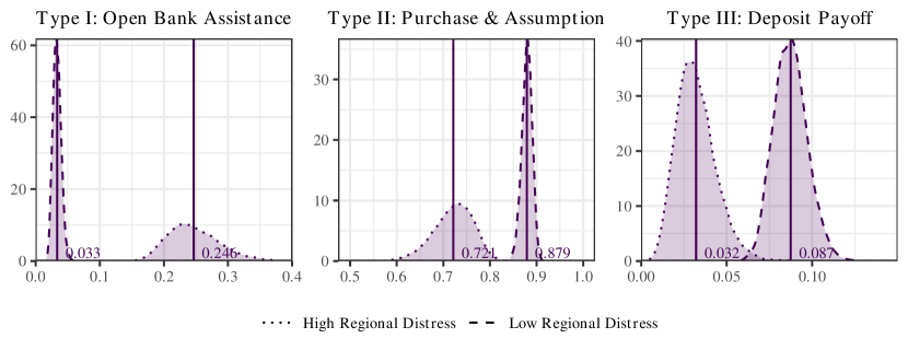
Figure 3: Posterior distribution of the average probability of the FDIC assigning each resolution method within classes based on regional distress. The horizontal axis represents the probability of assigning a resolution method and the vertical axis represents the posterior density associated with that probability based on a kernel density estimate. The solid vertical lines represent the means of these posterior distributions across the $G$ MCMC draws.

Figure 3 provides the density of the full posterior distribution of the average probability of receiving each resolution method across the two latent classes. The average probability of receiving a Type I resolution among HRD banks was 24.6% compared to 3.3% for LRD banks. The fully disjoint posterior densities of the average probability of receiving a Type I resolution for the HRD and LRD classes shows that the difference between their averages is statistically important. This observation continues to hold for Type II resolutions with statistically important differences in average resolution probabilities across HRD and LRD classes at 72.1% and 87.9% respectively. The theoretical recommendation from Cordella and Yeyati (2003) does not explicitly address the decision to facilitate partial or whole acquisitions of failed banks and the findings from this estimation exercise provide new insights into the differences in the probabilities of implementing the Type II resolution method under varying levels of economic distress. Finally, in a further confirmation of the predictions of the theoretical model, the average probability of being liquidated under a Type III resolution was 8.7% for LRD banks compared to 3.2% for HRD banks. This difference is also statistically important, as evidenced by the minimal overlap in posterior densities of the two classes.

4.1.3 Resolution Type

The next stage of the empirical analysis centers on the results from the ordinal probit models represented in Equation (7) and depicted in the second level of the decision structure in Figure 2. These models estimate separate relationships between the resolution method $y_{i}$ and bank-level financial indicators $\bm{x}_{i}$ in the LRD and HRD classes. If the FDIC responded differently to LRD and HRD failures for the same change in bank financial characteristics, this would manifest in different magnitudes of covariates across the two classes and provide conclusive evidence of the presence of two different decision rules implemented by the FDIC. In this section, we report the six largest covariate effects from the selected ordered response model (specification 3 in Table 1) in Figure 4. The covariate effects of the remaining variables are provided in Section F of the supplement.

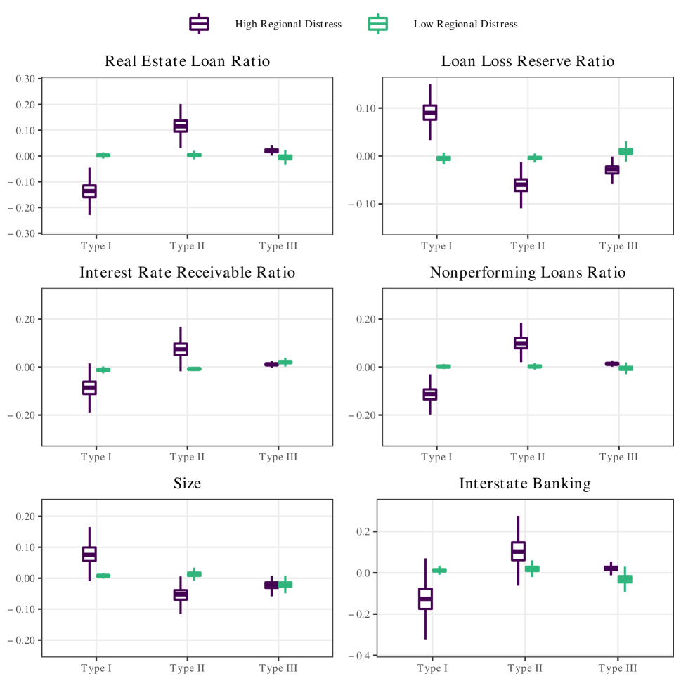
Figure 4: Covariate effects from the models for resolution type for banks in the class of High Regional Distress (HRD) and Low Regional Distress (LRD).

From Figure 4, the financial variables, Real Estate Loan Ratio and Nonperforming Loans Ratio, both exhibit qualitatively similar covariate effects. A unit standard deviation increase in Real Estate Ratio and Nonperforming Loans Ratio is associated with a reduced probability of obtaining assistance under a Type I resolution among HRD failures and an increased probability of such banks undergoing Type II and III resolutions. Since nonperforming loans provide a succinct measure of the quality of the failed bank’s assets and real estate loans represent a risky asset category, these results reveal that the FDIC provided assistance under Type I to banks that had relatively healthier balance sheets even among those banks that failed amid economic distress, which is consistent with the theoretical recommendations of Cordella and Yeyati (2003). The effects of these covariates on banks within the class of LRD failures, on the other hand, are not statistically important.

The Interest Receivable Ratio is seen to be important in the FDIC’s evaluation of bank health, with elevated levels of this ratio eliciting more stringent resolution methods from the FDIC. Balla et al. (2015) originally identified the Interest Receivable Ratio to be highly predictive of both bank failure and loss subsequent to failure in their study. Accordingly, an increase in Interest Receivable Ratio among HRD failures resulted in a reduction in the probability of Type I resolution and a corresponding increase in the probability of a Type II resolution, entailing partial or whole acquisitions of the failed institutions. Banks that belonged to the LRD class of failures experienced a more severe response in the form of an increased probability of a Type III resolution and hence, complete liquidation, along with a decreased probability of the other two resolution methods.

Larger banks were less likely to be liquidated under a Type III resolution across both latent classes. Among HRD failures, a standard deviation increase in log of assets was also associated with a decreased probability of a Type II resolution and a compensatory increase in the probability of assistance under Type I resolution. LRD failures experienced an increase in the probability of both, Type I and II resolutions concomitantly with a decrease in the probability of a Type III resolution. The increased probability of Type I resolutions associated with a larger bank reveals that the “too-big-to-fail” doctrine was present in the decisions of FDIC during the crisis of the 1980’s.

The estimation results provide new insights into the role of Loan Loss Reserve Ratio, an accounting variable that records the amount of funds set aside to meet expected losses. An increase in Loan Loss Reserves ratio was associated with a higher probability of receiving Type I resolution in the class of HRD failures. Contrarily, among LRD failures, an equivalent increase in this measure was associated with an increase in their probability of receiving a Type III resolution and being liquidated. A possible explanation for this disparity is that in the HRD class of banks, where failures are more likely to have occurred due to systemic factors, changes in loss reserve ratios can be attributed to the deterioration in asset quality resulting from market-wide fluctuations. However, among LRD failures, the FDIC is likely to have viewed the increase in this ratio as a signal of deterioration in asset quality arising from issues idiosyncratic to the failed bank.

Interstate is an indicator variable that identifies whether interstate banking was legal in the state in which a bank is located in the year of failure and is derived from summary tables in Strahan et al. (2003). Intuitively, interstate banking laws are likely to affect resolution outcomes as they determine the breadth of demand for assets of failed banks. For instance, the model in Acharya and Yorulmazer (2008) predicts that interstate banking, by expanding the set of available acquiring banks in the event of a failure, should be associated with an increase in the probability of a Type II resolution and an equivalent decline in the probability of a Type I resolution. In the bottom right panel of Figure 4, an increased probability of Type II resolutions is observed among both, HRD and LRD classes, even though the LRD class of failures also underwent a modest increase in the probability of Type I resolutions.

Overall, Figure 4 reveals that the magnitudes of the covariate effects from the selected model, specification (3), described in the preceding subsection, are larger for banks that belong to the latent class “High Regional Distress (HRD)” relative to banks in the class labeled “Low Regional Distress (LRD)”. This pronounced difference in the effects of each covariate on the FDIC’s decisions across the two classes confirms the presence of two distinct decision rules in the agency’s resolution procedure. The larger covariate effects for banks in the class of HRD failures indicate that within the group of banks that failed amid regional economic distress, the FDIC ordered banks based on their financial characteristics and provided Type I resolutions to relatively healthier banks and Type II and III resolutions to relatively weaker banks. The smaller covariate effects in the LRD class suggest that the FDIC evaluated banks that failed in low economic distress on a case-by-case basis rather than appraising their relative financial strength. This approach potentially included evaluating unobservable individual circumstances, which are captured by the error term in Equation (3). These results reveal a smaller role for observed financial statement information in determining resolution methods within the LRD class relative to the HRD class of banks and further support the hypothesis that banks in the former group are likely to have failed due to largely idiosyncratic factors.

5 Savings and loans resolution by FSLIC

The Federal Savings and Loans Insurance Corporation (FSLIC) insured S&L’s and served as a receiver for failed institutions, both of which were functions the FDIC performed within the banking industry. The FSLIC, however, was ultimately dissolved following unsustainable resolution losses that resulted in its insolvency in 1989. This section compares the decision rules of the FSLIC against theoretically recommended rules summarized in Section 1.2. To compare the FDIC with the FSLIC, we analyze the latter’s decisions through the same empirical lens and estimate the specifications described in Section 4 for FDIC decisions.

In Section 5.1 we discuss the results for hypotheses $H_{1}$ while the results pertaining to hypotheses $H_{2}$ and $H_{3}$ are presented in sections K and L of the supplement. The period under study covers the S&L failures that occurred over 1984-1989. The industry had also undergone an earlier wave of failures in the early 1980’s. Section I in the supplement provides an overview of the history of the crisis in the S&L industry and distinguishes between the two waves of S&L failures. In this analysis, we continue to use the same specifications as those described in Section 4 for the prior distributions, their hyperparameters and the number of post-burn in MCMC samples.

5.1 Regional economic distress and FSLIC’s decisions for S&L resolutions

We find that FSLIC’s designation of S&L institutions into classes based on regional economic distress is ambiguous and does not support Hypothesis $H_{1}$. The FSLIC’s decisions deviated from the decision structure implied by Hypothesis $H_{1}$ in a notable way. The agency did not develop distinct decision rules to resolve failures that occurred amid high and low regional distress and is observed to have adopted a common decision rule for both groups of S&L’s. The implication of using a common decision rule is that institutions that failed due to weaknesses in their own risk management as well as due to economic factors are likely to have received assistance with similar probabilities. The theory underlying this hypothesis suggests that by not fully disentangling economic and idiosyncratic factors while providing assistance, the FSLIC potentially fostered moral hazard among S&L institutions.

5.1.1 Class-membership model

Table 2 summarizes the covariate effects from estimating the specifications reported in Section 4.1.

Table 2: Covariate effects from class-membership models of S&L’s for specifications of latent classes based on regional distress. The reported values are posterior means of the covariate effects. Posterior standard deviations are in parantheses.

	(1†)	(2†)	(3†)	(4†)
State-level characteristics
Unemployment	-0.08 (0.06)	-0.71 (0.14)	-0.17 (0.48)	-0.72 (0.11)
Housing starts	-0.21 (0.1)	-0.01 (0.04)	-0.03 (0.09)	-0.02 (0.04)
County-level characteristics
Per capita GDP growth	-0.13 (0.09)	0.02 (0.06)	0.00 (0.09)	0.01 (0.05)
Farm, agri, mining	-0.09 (0.08)	0.04 (0.04)	-0.01 (0.09)	0.04 (0.03)
Manufacturing	0 (0.07)	-	-	-
Construction	0.09 (0.05)	-	-	-
Fin Serv Transport	-0.11 (0.12)	-	-	-
Government	-0.16 (0.1)	-	-	-
Insurer characteristics
Dep. Ins. Fund/Total Dep.	-	-	0.01 (0.08)	-
S&L-level characteristics
State charter	-	-	-	-0.07 (0.15)
log Marginal Likelihood	-302.32	-305.40	-302.02	-305.44

Specification (3^†) is determined to be the model selected by the data by virtue of its marginal likelihood being the largest among candidate models. The covariate effects for unemployment, per capita income and housing starts in this specification are, however, not statistically important. Accordingly, the latent classes generated by this model cannot be distinguished as representing “high” or “low” regional distress and are labeled as “Regional Distress Class 1” and “Regional Distress Class 2”.

5.1.2 Heterogeneity in Decision Rules

Figure 5 shows the posterior densities of the average probability of the FSLIC assigning each resolution method to S&L’s in the two latent classes. These distributions offer two main insights into the decisions of the FSLIC. First, on comparing with Figure 3, it is clear that the FSLIC relied more heavily on Type I resolutions relative to the FDIC. The average probabilities of the FSLIC assigning a Type I resolution were 67.5 % and 69.6% in class 1 and 2 compared with probabilities of 24.6 % and 3.3% of the FDIC assisting banks that failed in high and low regional distress respectively. Second, the FSLIC recognizably deviated from the recommended resolution strategy developed in Cordella and Yeyati (2003) since the posterior densities for the two classes overlap across all three resolution methods. Accordingly, the average probabilities of receiving a Type I resolution are not statistically different across the two classes. This finding signifies that the FSLIC did not distinguish between S&L institutions that failed amid high and low economic distress in assigning Type I assistance.

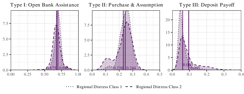
Figure 5: Posterior distribution of the average probability of the FSLIC assigning each resolution method within classes based on regional distress. The horizontal axis represents the probability of assigning a resolution method and the vertical axis represents the posterior density associated with that probability based on a kernel density estimate. The solid vertical lines represent the mean of these posterior distributions across the $G$ MCMC draws.

5.1.3 Resolution Type

Figure 6: Covariate effects from the models for resolution type for S&L’s in the classes based on regional distress.

The box plots for covariate effects from specification (3^†) in Figure 6 show that the FSLIC adopted a common decision rule in resolving institutions in the two classes. The covariate effects of S&L financial characteristics are homogeneous across the two latent classes. This contrasts with the covariate effects on the FDIC’s responses in Figure 4, which are statistically different across the classes of banks that failed amid high and low regional distress. In both latent classes in the FSLIC’s decision structure, a standard deviation increase in Real Estate Loan Ratio is seen to result in an average decline of around 7% in the probability of receiving a Type I resolution and a corresponding increase in the probability of receiving the other two resolution methods. Since real estate prices collapsed across several regions during this period, institutions with excess concentrations in real estate lending would have been exposed to heightened risks of defaults and losses. Thereby, the FSLIC likely considered such institutions to be incapable of being revived through assistance. Between the two latent classes, the FSLIC responded to Larger Loan Loss Reserve Ratios among institutions in “Regional Distress Class 2” by withholding assistance and instead facilitating their acquisition or liquidating them. This response is similar but more muted in “Regional Distress Class 1”. This suggests that the FSLIC viewed larger loss reserves as a signal of greater deterioration in the asset quality of the failed institution.

The FSLIC did not respond to changes in the Interest Rate Receivable Ratio, which has been shown to be correlated with the losses resulting from the failed institution to the resolution agency (Balla et al., 2015). The average change in the probability of assigning each resolution method is close to zero in response to a standard deviation increase in this measure. This finding suggests that the FSLIC did not distinguish across institutions that held larger or smaller shares of loans on which payments were past due, on which interest accrues and is thereby included in our measure of receivable interest. The FSLIC’s decisions with respect to bank size were similar to those of the FDIC. Larger institutions were more likely to be assisted by the agency and less likely to be sold or liquidated across both latent classes, thereby reflecting the “too-big-to-fail” doctrine in the agency’s decisions. The FSLIC assigned Type I assistance to a greater extent in states where interstate banking was permitted, but this effect was solely present in class 1. Average covariate effects were close to zero for all three resolution types in class 2. The variable “Interstate banking” pertains only to the deregulation within the banking industry as the S&L industry was not subject to such restrictions (Roster, 1985). Since S&L’s would have faced more intense competition from the banking industry in states where interstate banking was permitted, the FSLIC likely provided assistance with greater probability in such states as such competition would have adversely affected even those S&L’s that were healthy. The covariate effects of the remaining variables are provided in Section J of the supplement.

Overall, the FSLIC’s decision rules did not differ by the extent of regional distress that accompanied the failure of S&L’s. Moreover, the covariate effects in the ordinal models for the FSLIC’s decisions on resolution types were lower in magnitude relative to the equivalent values for the FDIC’s decisions. These findings suggest that the FSLIC did not adhere to the recommendation from theoretical studies of assigning S&L’s to distinct decision rules depending on whether the failure was likely related to broader economic factors or the institution’s idiosyncratic weaknesses. In addition, the FSLIC relied on S&L’s financial characteristics to a lesser extent than the FDIC in undertaking resolution decisions, thereby suggesting that the agency assigned resolution methods on a case-by-case basis rather than by adopting a consistent data-driven rule.

6 Discussion and contemporary relevance

During banking crises, financial regulators intervene to bail out certain failed institutions and liquidate others. Regulators are expected to meet the dual objectives of preserving financial stability and discouraging moral hazard in the process of reaching such decisions. However, they may deviate from socially optimal resolution decisions. Furthermore, as bailouts typically entail transfers from taxpayers to bank depositors and equity holders, these actions evoke public disapproval even when they are carried out in the public interest. The risk of regulatory transgressions creates a need for the public to regularly evaluate regulators’ actions. Additionally, in order to mitigate biases in assessments from unduly strong subjective beliefs against public assistance or liquidation, an objective framework of assessment is essential.

An important line of inquiry in assessing the appropriateness of resolution decisions consists of evaluating whether regulatory agencies applied two different decision rules for bank failures amid economic distress and under normal economic conditions. Since the true classification of banks into distinct decision protocols is unobservable, we have developed a Bayesian latent class estimation framework to detect unobserved heterogeneity in the resolution decisions of banks based on underlying economic conditions. This flexible estimation approach permits inferences on whether the decision rules across the latent classes are statistically different. Bayesian model comparison exercises predicated on posterior odds inform the selection of models that best explain the decision rules of regulatory agencies.

We utilize this modeling framework to assess the responses of the FDIC and the FSLIC to bank and S&L failures respectively during the crises of the 1980’s in the two industries. Our results show that the decision rules of the FSLIC, which subsequently faced insolvency at a significant cost to taxpayers, were inconsistent with the decision rules recommended by theoretical studies that address the trade-offs between financial stability and moral hazard. The FDIC, which survived the earlier crisis as well as the financial crisis of 2008, was found to have undertaken decisions that were consistent with those recommended rules. These findings consequently validate the applicability of this approach to assess regulators.

Were there structural differences between the FDIC and FSLIC that contributed to these distinct resolution strategies? First, diluted standards for closing S&L institutions implied that the financial position of S&L’s was more critical than that of banks at the time of failure. Second, deregulation and forbearance resulted in a deeper crisis in the S&L industry than in the banking industry (9% S&L failures relative to 2% bank failures). Following deregulation in the mid-1980’s, S&L’s that previously operated purely within the retail loan and deposit market were permitted entry into the commercial loan market. Despite their entry into a line of business that was historically serviced by banks, capital requirements were lower for S&L’s than they were for banks. This forbearance resulted in the rapid expansion of the S&L industry accompanied by augmented risk-taking, which ultimately led to widespread failures.

A regular assessment of resolution authorities by lawmakers and the public can uncover gaps between observed and recommended resolution rules and also point out the source of such gaps. Assessments of the FSLIC could have revealed the issues arising from deregulation of the S&L industry and prompted a review of the structure of the agency, preventing both, the failure of the agency and the ensuing costs to the taxpayer. The insights from this study can potentially guide the development of resolution strategies among newer resolution agencies such as the Single Resolution Board under the European Central Bank.

Supplementary materials – Do financial regulators act in the public’s interest? A Bayesian latent class estimation framework for assessing regulatory responses to banking crises

This supplement is organized as follows. Section A includes additional details about the data used in this paper, Section B provides a simulation study to assess the performance of the collapsed Gibbs sampler discussed in Section 3.6, Section C provides the full Gibbs sampler for posterior inference in the our latent class ordinal model of Section 3, Section D describes the calculation of covariate effects and Section E provides additional details about model comparison. Sections F, G and H include, respectively, additional covariate effects, and results for hypotheses $H_{2},~{}H_{3}$ pertaining to FDIC’s resolution decisions. The corresponding discussion related to FSLIC’s resolution decisions are provided in Sections I (history of S&L failures), J (additional covariate effects), K (results for hypothesis $H_{2}$) and L (results for hypothesis $H_{3}$).

Appendix A Summary statistics and description of bills

Table 3 provides the data dictionary and Tables 4, 5 present descriptive statistics of the data described in Section 2.

In this paper, we consider the following five bills that were favorable to the banking or S&L industry.

1. Bill 1 - reform, recapitalize and consolidate the federal deposit insurance system as well as to enhance the powers of federal regulatory agencies.

2. Bill 2 - introduce additional checks on the banking industry by proposing the restoration of civil penalties for criminal offenses involving financial institutions

3. Bill 3 - restructure the S&L industry and recommended that the FDIC insure deposits held at S&L institutions in addition to commercial banks following the failure of the FSLIC. This bill also authorized the establishment of the Resolution Trust Corporation (RTC) to resolve failed S&L institutions that had been within the purview of the FSLIC and any additional failures that arose within the next three years.

4. Bill 4 - The Competitive Equality Bank Act (CEBA) of 1987 provided the FDIC with the option to establish a temporary national bank or a bridge bank for a maximum period of three years. This option served as an alternative to liquidation when acquirers were not forthcoming for purchasing a bank in the period immediately following its failure (Huber, 1988)

5. Bill 5 - disclosure of ratings assigned to banks and thrifts under the Community Reinvestment Act (CRA).

With the exception of Bill 4, all other bills described above are components of the Financial Institutions Reform, Recovery and Enforcement Act(FIRREA) of 1989. In tables 4 and 5, the category ‘% vote for Bill $k$’ represents the percentage of Congressional representatives from the state in which the bank (S&L) operated who voted for bill $k$ that was favorable to the banking or S&L industry, where $k=1,\ldots,5$.

Table 3: The data dictionary. All state level and county level characteristics pertain to those U.S. states and counties where the banks (S&L’s) failed during the crises of 1980’s.

Covariates Description Bank and S&L level characteristics C&I Loan Ratio ratio of commercial and industrial loans to total loans CLD Loan Ratio ratio of construction and land development loans to total loans Real Estate Loan Ratio ratio of real estate loans to total loans Loan Loss Reserves Ratio ratio of reserves set aside against expected losses to total loans Nonperforming loans Ratio (for banks) ratio of loans past due and loans in non-accruing status to total assets Interest Receivable Ratio ratio of interest income earned but not collected to total assets Securities Ratio ratio of securities (e.g., Treasuries, mortgage-backed securities) to total assets Core Deposits Ratio (for banks) ratio of the sum of transaction deposits of individuals, governments, corporations, money market deposit accounts, and time deposits with balances less than $100,000 relative to total liabilities Earnings (for banks) ratio of net income to total assets Size(Assets mlns.) total assets in millions of dollars State charter Fed member (for banks) indicator depicting state-chartered banks that are members of the Federal Reserve system State charter non-Fed member (for banks) indicator depicting state-chartered banks that are not members of the Federal Reserve system State charter (for S\&L’s) indicator depicting state-chartered S&L’s Insurer characteristic Dep. Ins. Fund/ Total Deposits ratio of insurance funds available to total deposits State Characteristics Interstate banking whether interstate banking is legal in the state in which the bank (S&L) failed Unemployment unemployment rate in the state in which the bank (S&L) failed Housing starts number of new house constructions in the state in which the bank (S&L) failed County characteristics Per capita GDP growth per capita year-on-year growth of county GDP Farm, Agri and Mining quarterly share of employment in farming, agriculture and mining Manufacturing quarterly share of employment in manufacturing Construction quarterly share of employment in construction Fin Serv and Transport quarterly share of employment in financial services and transportation Government quarterly share of employment in government County-level characteristics of bank distress % Assets in Banks with Texas Ratio $>$ 100% percent of assets in banks with Texas Ratio $>$ 100% relative to total banking assets in the county % Deposits in Banks with Texas Ratio $>$ 100% percent of deposits in banks with Texas Ratio $>$ 100% relative to total bank deposits in the county % banks with Texas Ratio $>$ 100% percent of banks in the county with Texas Ratio $>$ 100% Previous Closures number of bank (S&L) closures in the county in the previous year State-level political economy characteristics % Republicans in 1987 % of Republicans in Congress in 1987 % Republicans in 1989 % of Republicans in Congress in 1989 % vote for Bill 1: enhancing reg. agencies powers % of Congressional votes in favor of Bill 1 % vote for Bill 2: restoring civil penalties for fin. Inst. % of Congressional votes in favor of Bill 2 % vote for Bill 3: recommitting S&L restructuring bill % of Congressional votes in favor of Bill 3 % vote for Bill 4: CEBA % of Congressional votes in favor of Bill 4 % vote for Bill 5: disclosure of CRA ratings % of Congressional votes in favor of Bill 5

Table 4: Descriptive statistics of bank, county and state-level characteristics in the data sample for FDIC resolution decisions. See Section A of the supplement for a description of the bills evaluated in this analysis under the state-level political economy characteristics.

Type I (OBA) Type II (P&A) Type III (PO) Mean Std. dev Mean Std. dev Mean Std. dev Bank-level characteristics C&I Loan Ratio 27% 13% 27% 16% 28% 16% CLD Loan Ratio 6% 8% 5% 7% 4% 8% Real Estate Loan Ratio 39% 17% 42% 21% 31% 20% Loan Loss Reserves Ratio 6% 6% 4% 3% 5% 7% Nonperforming loans Ratio 6% 6% 8% 5% 8% 6% Interest Receivable Ratio 1% 1% 1% 1% 2% 1% Securities Ratio 12% 12% 13% 10% 14% 11% Core Deposits Ratio 63% 18% 73% 13% 74% 15% Earnings -3% 6% -3% 4% -4% 4% Size(Assets mlns.) 212 654 171 893 47 96 State charter Fed member 4% 20% 7% 26% 14% 35% State charter non-Fed member 50% 50% 53% 50% 48% 50% Insurer characteristic Dep. Ins. Fund/ Total Deposits 14% 11% 16% 23% 10% 20% State Characteristics Interstate branching 0.86 0.34 0.77 0.42 0.51 0.50 Unemployment 8% 1% 7% 2% 6% 1% Housing starts 13% 7% 11% 13% 16% 17% County characteristics Per capita GDP growth 3% 3% 5% 5% 6% 7% Farm, Agri and Mining 8% 8% 11% 11% 16% 14% Manufacturing 11% 5% 11% 7% 8% 5% Construction 6% 1% 5% 2% 5% 2% Fin Serv and Transport 39% 7% 36% 9% 36% 11% Government 15% 6% 16% 7% 16% 6% County-level characteristics of bank distress % Assets in Banks with Texas Ratio $>$ 100% 13% 16% 5% 11% 7% 15% % Deposits in Banks with Texas Ratio $>$ 100% 12% 13% 5% 11% 7% 15% % banks with Texas Ratio $>$ 100% 8% 8% 6% 9% 7% 11% Previous Closures 4.00 6.27 2.62 6.15 1.54 4.72 Count 118 - 1175 - 92 - State-level political economy characteristics % Republicans in 1987 41% 12% 43% 17% 52% 22% % Republicans in 1989 35% 14% 40% 18% 47% 19% % vote for Bill 1: enhancing reg. agencies powers 83% 14% 80% 21% 83% 18% % vote for Bill 2: restoring civil penalties for fin. Inst. 93% 20% 88% 23% 82% 28% % vote for Bill 3: recommitting S&L restructuring bill 97% 2% 98% 3% 98% 3% % vote for Bill 4: CEBA 99% 3% 98% 5% 98% 4% % vote for Bill 5: disclosure of CRA ratings 33% 17% 37% 23% 33% 26% Count 118 - 1170 - 92 -

Table 5: Descriptive statistics of S&L, county and state-level characteristics in the data sample for FSLIC resolution decisions. See Section A of the supplement for a description of the bills evaluated in this analysis under the state-level political economy characteristics.

Type I (OBA) Type II (P&A) Type III (PO) Mean Std. dev Mean Std. dev Mean Std. dev S&L-level characteristics C&I Loan Ratio 3% 5% 4% 6% 5% 9% CLD Loan Ratio 14% 20% 27% 25% 20% 25% Real Estate Loan Ratio 93% 11% 96% 17% 103% 20% Loan Loss Reserves Ratio 5% 8% 9% 11% 4% 5% Interest Receivable Ratio 1% 1% 2% 3% 2% 1% Securities Ratio 20% 15% 13% 9% 12% 10% Size(Assets mlns.) 471 1961 316 484 201 243 State charter 11% 31% 8% 27% 7% 25% Insurer characteristic Dep. Ins. Fund/ Total Deposits -1% 18% 0% 22% 7% 22% State Characteristics Interstate branching 0.69 0.46 0.54 0.50 0.33 0.47 Unemployment 8% 2% 8% 2% 8% 2% Housing starts 16% 17% 19% 22% 23% 25% County characteristics Per capita GDP growth 4% 4% 4% 4% 6% 3% Farm, Agri and Mining 7% 8% 8% 8% 9% 7% Manufacturing 14% 8% 13% 7% 14% 7% Construction 5% 3% 5% 2% 5% 1% Fin Serv and Transport 37% 8% 37% 9% 34% 10% Government 15% 6% 16% 7% 20% 15% Count 270 - 104 - 15 - County-level characteristics of S&L distress % Assets in Banks with Texas Ratio $>$ 100% 3% 8% 2% 5% 3% 6% % Deposits in Banks with Texas Ratio $>$ 100% 3% 8% 2% 5% 3% 6% % banks with Texas Ratio $>$ 100% 4% 8% 3% 7% 3% 5% Previous Closures 0.24 0.29 0.27 0.56 0.76 0.77 Count 270 - 102 - 15 - State-level political economy characteristics % Republicans in 1987 41% 11% 41% 15% 43% 10% % Republicans in 1989 35% 14% 40% 18% 47% 19% % vote for Bill 1: enhancing reg. agencies powers 83% 14% 80% 21% 83% 18% % vote for Bill2: restoring civil penalties for fin. Inst. 93% 20% 88% 23% 82% 28% % vote for Bill 3: recommitting S&L restructuring bill 97% 2% 98% 3% 98% 3% % vote for Bill 4: CEBA 97% 5% 97% 6% 94% 6% % vote for Bill 5: disclosure of CRA ratings 33% 17% 37% 23% 33% 26% Count 267 - 103 - 15 -

Appendix B Simulation Study

In this simulation study we assess the performance of the Collapsed Gibbs sampler of Section 3.6 for posterior inference in our latent class ordinal model. We consider two simulation settings, the first of which contains latent classes with disparate means and the other, in which the means overlap. To evaluate the algorithm’s accuracy in recovering parameters, we generate differences in means by considering alternative values of coefficients $\bm{\beta}_{s},s\in\{1,2\}$ across the two settings, and leave the covariates unchanged. The simulation exercise has been performed on a sample of size $n=1200$ observations under both the settings with $p=2$ and $q=4$. In each setting, the first component of the covariates $\bm{w}_{i},~{}i=1,\ldots,n$ is an intercept and the second component is drawn independently from a standard normal distribution. Similarly, in the ordinal model, the first component of the covariates $\bm{x}_{i}$ is an intercept, and the second, third and fourth components are drawn independently from $\mathcal{N}(0.5,1)$, $\mathcal{N}(0.5,1)$ and $\mathcal{N}(0,0.8)$ respectively. The true values of parameters in the two settings are provided in the second column of Table 6. Under these specifications, the mean under the two latent classes for the two settings are obtained as follows:

• Setting 1: $\sum_{i=1}^{n}\bm{x}_{i}^{\prime}\bm{\beta}_{1}\mathbb{I}\{s_{i}=1\}/\sum_{i=1}^{n}\mathbb{I}\{s_{i}=1\}=-0.04$, $\sum_{i=1}^{n}\bm{x}_{i}^{\prime}\bm{\beta}_{2}\mathbb{I}\{s_{i}=2\}/\sum_{i=1}^{n}\mathbb{I}\{s_{i}=2\}=-0.52$.

• Setting 2: $\sum_{i=1}^{n}\bm{x}_{i}^{\prime}\bm{\beta}_{1}\mathbb{I}\{s_{i}=1\}/\sum_{i=1}^{n}\mathbb{I}\{s_{i}=1\}=0.01$, $\sum_{i=1}^{n}\bm{x}_{i}^{\prime}\bm{\beta}_{2}\mathbb{I}\{s_{i}=2\}/\sum_{i=1}^{n}\mathbb{I}\{s_{i}=2\}=-0.02$.

We continue to use the same prior distributions and hyperparameters as those specified in Section 4.

Table 6: Credibility intervals from simulation studies based on two parameter specifications

	Setting 1: Disparate Means		Setting 2: Common Means
	True Values	Cred. Int.	True Values	Cred. Int.
	Class Membership
$\alpha_{1}$	-0.3	[-0.42,-0.26]	-0.3	[-0.50,-0.22]
$\alpha_{2}$	1.5	[1.29,1.53]	1.5	[1.14,1.48]
	Latent class 1
$\beta_{11}$	0.6	[0.57,0.64]	0.6	[0.59,0.67]
$\beta_{21}$	-0.7	[-0.69,-0.61]	-0.6	[-0.67,-0.57]
$\beta_{31}$	-0.6	[-0.62,-0.53]	-0.6	[-0.69,-0.60]
$\beta_{41}$	0.5	[0.48,0.58]	0.5	[0.48,0.57]
$\sigma_{1}^{2}$	0.25	[0.20,0.27]	0.25	[0.22,0.29]
	Latent class 2
$\beta_{12}$	0.1	[0.06,0.17]	0.1	[-0.03,0.08]
$\beta_{22}$	0.6	[0.56,0.66]	-0.1	[-0.12,-0.04]
$\beta_{32}$	0.2	[0.18,0.26]	-0.1	[-0.11,-0.02]
$\beta_{42}$	0.8	[0.79,0.94]	0.8	[0.79,0.92]
$\sigma_{2}^{2}$	0.25	[0.21,0.29]	0.25	[0.17,0.24]

Table 6 summarizes the one-standard deviation credibility intervals from the estimation of all parameters under the two specifications. The two-standard deviation credibility intervals, not shown here, contain the true values for all parameters under both settings. The more conservative one-standard deviation credibility intervals under Setting 1 contain the true values of parameters with the exception of $\beta_{21}$, for which the credibility interval lies marginally above the true value. Under Setting 2, the true values of parameters lie marginally beyond credibility intervals for $\alpha_{2}$, $\beta_{12}$ and $\sigma_{2}^{2}$. The credibility intervals are also narrower under Setting 1 relative to Setting 2, demonstrating the enhanced precision of estimates under more separated classes.

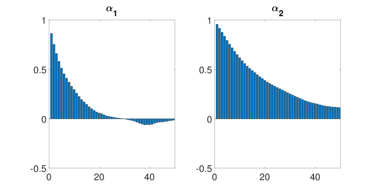
Figure 7: Autocorrelation in the posterior sample of $\bm{\alpha}=(\alpha_{1},\alpha_{2})$ from a full Gibbs sampler under simulation Setting 1. The full Gibbs sampler algorithm is available in Section C of the supplement. Here $\alpha_{1}$ is the intercept and $\alpha_{2}$ is the coefficient of the second component of $\bm{w}_{i}$ within the class membership model considered in this simulation exercise.

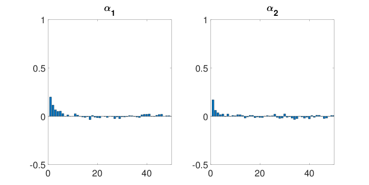
Figure 8: Autocorrelation in the posterior sample of $\bm{\alpha}=(\alpha_{1},\alpha_{2})$ from the collapsed Gibbs sampler (Section 3.6) under simulation Setting 1. Here $\alpha_{1}$ is the intercept and $\alpha_{2}$ is the coefficient of the second component of $\bm{w}_{i}$ within the class membership model considered in this simulation exercise.

Figures 7 and 8 display the autocorrelations in the posterior samples of $\bm{\alpha}$ under a full Gibbs sampler (Section C) and the proposed Collapsed Gibbs sampler (Section 3.6), respectively, for Setting 1. The figures show that the reduction in autocorrelations gained from the latter method is striking. The autocorrelations from the full Gibbs sampler are close to 1 at lower lags and decay slowly whereas the autocorrelations from the Collapsed Gibbs sampler are negligible even at lower lags and taper to zero within 5 lags. This demonstrates that the proposed Collapsed Gibbs sampler algorithm introduced in Section 3.6 provides an efficient technique for sampling from the posterior distribution relative to standard sampling approaches by reducing autocorrelations across successive draws.

The results from this simulation exercise have been corrected for label-switching using Papastamoulis (2016). This issue affects MCMC algorithms constructed for the estimation of finite mixture models and results in switching of class labels in the course of the chain. The class labels have been reassigned post-estimation using an ordering constraint on the intercept in both classes.

Appendix C Full Gibbs sampler

Here we present the full Gibbs sampler algorithm for posterior inference in the latent class ordinal model discussed in Section 3.
 
Algorithm: Full Gibbs Sampler

1. Sample $\bm{\beta}_{s}$ from the distribution $\bm{\beta}_{s}|\bm{z},\bm{u},\sigma^{2}_{s}$ for $s=1,2$.

2. Sample $\sigma^{2}_{s}$ from $\sigma^{2}_{s}|\bm{\beta}_{s},\bm{z},\bm{u}$ for $s=1,2$.

3. 1. Sample $\bm{\alpha}$ from $\bm{\alpha}|\bm{u},\bm{\beta},\bm{\sigma}^{2},\bm{y}$, where $\bm{\beta}=(\bm{\beta}_{1},\bm{\beta}_{2})$ and $\bm{\sigma}^{2}=(\sigma_{1}^{2},\sigma_{2}^{2})$.

   2. Sample $l_{i}|\bm{\alpha},\bm{u}$, where for $i=1,\ldots,n$.

4. Sample $s^{\prime}_{i}$ from $s^{\prime}_{i}|\bm{\alpha},\bm{\beta},\bm{\sigma}^{2},\bm{y}$ for $i=1,\ldots,n$.

5. Sample $z_{i,s_{i}}$ from $z_{i,s_{i}}|\bm{\beta},\bm{\sigma}^{2},\bm{y},\bm{u}$ for $i=1,\ldots,n$.

Steps (a), (b), (d) and (e) are identical to the algorithm described in Section 3.6. Step (c) of this algorithm is described below.
 
Sampling coefficients $\bm{\alpha}$ of the Class Membership Model - (i) The coefficients $\bm{\alpha}$ of the class membership model are sampled from the full conditional $\mathcal{N}(\hat{\bm{\alpha}}_{0},\hat{A})$ where $\hat{A}=(A_{0}+W^{\prime}W)^{-1}$, $\hat{\bm{\alpha}}_{0}=\hat{A}(A_{0}^{-1}\bm{\alpha}_{0}+W^{\prime}l)$ and $W$ is the $n\times p$ matrix that has the vector of $p$-dimensional covariates $\bm{w}_{i}^{\prime}$ from Equation (2) in its rows.

(ii) The latent variable $l_{i}$ is sampled using the data augmentation approach in Albert and Chib (1993) and drawing from the full conditional distribution, which is a truncated normal distribution with mean $\bm{w}_{i}^{\prime}\bm{\alpha}$, variance $1$ and region of truncation $\mathcal{C}_{i}$, where

$$\mathcal{C}_{i}=\begin{cases}(0,\infty),&\text{if}\ s_{i}=2\\ \left(-\infty,0\right]&\text{if}\ s_{i}=1\\ \end{cases}.$$

Appendix D Covariate Effects

An intuitive interpretation of the relationship between covariates and outcomes is provided by covariate effects in models with discrete dependent variables. Here, we discuss the calculation of covariate effects for the resolution-type model, the second level model in Figure 2. Consider any covariate, $x_{k}\in\mathcal{X}=(x_{1},\ldots,x_{q})$, whose effects on the outcome $y$ marginally of the other variables in $\mathcal{X}$ is of interest. Denote $\mathcal{X}_{\setminus k}$ to be the $q-1$ dimensional covariate vector obtained by excluding the $k^{th}$ covariate for $k=1,\ldots,q$ and let $\bm{\theta}_{s}=(\bm{\alpha},\bm{\beta}_{s},\sigma_{s}^{2})$. In our resolution-type model, the covariate effect measures the change in the marginal probability of observing $y=j$ for a given change in $x_{k}$ conditional on latent class $s$.

The framework for computing covariate effects while addressing both data variability and parameter uncertainty described in Jeliazkov and Vossmeyer (2018) has been adapted to the latent class model for ordinal outcomes. Each of these issues is overcome by averaging over the sample and the posterior distribution of parameters respectively. Equation (11) details how the output from the MCMC algorithm developed in Section 3.6, which consists of $G$ draws from the posterior distribution of parameters, is used in evaluating covariate effects for each of the two latent classes. We have, for $s\in\{1,2\}$,

$$\begin{split}Pr(y=j|{x_{k}^{\dagger}},s)-Pr(y=j|{x_{k}^{\ddagger}},s)=&\int\Bigl{\{}Pr(y=j|{x_{k}^{\dagger}},\mathcal{X}_{\setminus k},\bm{\theta}_{s})\\ -&Pr(y=j|{x_{k}^{\ddagger}},\mathcal{X}_{\setminus k},\bm{\theta}_{s})\Bigr{\}}f(\mathcal{X}_{\setminus k})f(\bm{\theta}_{s}|y)\mbox{d}\mathcal{X}_{\setminus k}\mbox{d}\bm{\theta}_{s}\\ \approx&\frac{1}{nG}\sum_{i=1}^{n}\sum_{g=1}^{G}\Bigl{\{}Pr\left(y_{i}=j|{x_{ik}^{\dagger}},\bm{x}_{i,\setminus k},\bm{\theta}_{s}^{(g)}\right)\\ -&Pr\left(y_{i}=j|{x_{ik}^{\ddagger}},\bm{x}_{i,{\setminus k}},\bm{\theta}_{s}^{(g)}\right)\Bigr{\}}\end{split}$$ (11)

where $\bm{x}_{i,\setminus k}$ denotes the $i^{th}$ row of $X$ excluding the $k^{th}$ element. The probabilities in the parentheses in the final step of Equation (11) are obtained by using the expression in Equation (7).

Appendix E Model Comparison

Subsequent to estimating the model, the empirical objective is to then identify the specification of the model that is corroborated by the data most decisively. Accordingly, this section presents the procedure for the comparison of posterior probabilities of estimated models. This is a method of model comparison that conforms to the Bayesian principle of representing uncertainty in the form of probability statements. Specifically, in comparing models $\mathcal{M}_{i}$ and $\mathcal{M}_{j}$, the posterior odds ratio, $\mathcal{P}_{ij}$, is evaluated to select between the pair of models, where,

$$\mathcal{P}_{ij}=\frac{P(\mathcal{M}_{i}|\bm{y})}{P(\mathcal{M}_{j}|\bm{y})}=\frac{m(\bm{y}|\mathcal{M}_{i})}{m(\bm{y}|\mathcal{M}_{j})}\frac{P(\mathcal{M}_{i})}{P(\mathcal{M}_{j})}.$$

The first term on the right hand side of the second equality is the Bayes factor and the second term is the prior odds. The Bayes factor is the ratio of marginal likelihoods of models $i$ and $j$ and following standard convention in which the $a$ $priori$ probability of each model occurring is equal, this quantity singularly determines the evidence in favor of one model against the other. Therefore, Bayesian model selection among $L$ models, $\{\mathcal{M}_{1},\mathcal{M}_{2},...,\mathcal{M}_{L}\}$, proceeds by comparing the marginal likelihood across these models.

The basic marginal likelihood identity recognized by Chib (1995) allows for the exact evaluation of the marginal likelihood by MCMC methods. This identity expresses the marginal likelihood of model $l$ as

$$m(\bm{y}|\mathcal{M}_{l})=\frac{f(\bm{y}|\mathcal{M}_{l},\bm{\theta}_{l})\pi(\bm{\theta}_{l}|\mathcal{M}_{l})}{\pi(\bm{\theta}_{l}|\bm{y},\mathcal{M}_{l})},$$

where $\bm{\theta}_{l}$ is a parameter vector specific to model $l$. The computation of the marginal likelihood simply requires the evaluation of this ratio for a given $\bm{\theta}_{l}^{*}$, typically the posterior mean or mode. The likelihood $f(\bm{y}|\mathcal{M}_{l},\bm{\theta}_{l})$ and prior ordinate $\pi(\bm{\theta}_{l}|\mathcal{M}_{l})$ at $\bm{\theta}_{l}^{*}$ can be evaluated analytically for the latent class model with ordered outcomes. The posterior ordinate $\pi(\bm{\theta}_{l}|\bm{y},\mathcal{M}_{l})$ at $\bm{\theta}_{l}^{*}$ is estimated to obtain $\hat{\pi}(\bm{\theta}_{l}^{*}|\bm{y},\mathcal{M}_{l})$ using methods outlined in Chib and Jeliazkov (2001) and Chib (1995).

E.1 Evaluating the Marginal Likelihood

Here we present the algorithm to evaluate the estimated posterior ordinate $\hat{\pi}(\bm{\theta}^{*}_{l}|\bm{y},\mathcal{M}_{l})$. Henceforth, we will drop the subscript $l$ for notational ease.

In the latent class model $\mathcal{M}$ with ordered outcomes, the parameter vector $\bm{\theta}$, excluding any latent variables, consists of the coefficients $\bm{\alpha},\bm{\beta}=(\bm{\beta}_{1},\bm{\beta}_{2})$ and the error variances $\bm{\sigma}^{2}=(\sigma_{1}^{2},\sigma_{2}^{2})$. The objective of this exercise is to evaluate the posterior ordinate at the posterior mean, $\bm{\theta}^{*}=(\bm{\alpha}^{*},\bm{\beta}^{*},\bm{\sigma}^{2*})$. The law of total probability is used to decompose the posterior ordinate at $\bm{\theta}^{*}$ as,

$$\pi(\bm{\alpha}^{*},\bm{\beta}^{*},\bm{\sigma}^{2*}|\bm{y},\mathcal{M})=\pi(\bm{\alpha}^{*}|\bm{y},\mathcal{M})\pi(\bm{\beta}^{*}|\bm{\alpha}^{*},\bm{y},\mathcal{M})\pi(\bm{\sigma}^{2*}|\bm{\alpha}^{*},\bm{\beta}^{*},\bm{y},\mathcal{M})$$

The order of this decomposition has been chosen to minimize computational time and effort. The first component, $\pi(\bm{\alpha}^{*}|\bm{y},\mathcal{M})$ is estimated using the method introduced in Chib and Jeliazkov (2001). By conditioning the other two densities on $\bm{\alpha}^{*}$, these ordinates can be estimated using reduced Gibbs samplers described in Chib (1995). The following reduced Gibbs sampler provides the estimated ordinate $\hat{\pi}(\bm{\beta}^{*}|\bm{\alpha}^{*},\bm{y},\mathcal{M})$.

1. Sample $\bm{\beta}_{s}$ from the distribution $\bm{\beta}_{s}|\bm{z},\bm{u},\bm{\sigma}^{2}_{s}$ for $s=1,2$.

2. Sample $\bm{\sigma}^{2}_{s}$ from $\bm{\sigma}^{2}_{s}|\bm{\beta}_{s},\bm{z},\bm{u}$ for $s=1,2$.

3. Sample $s^{\prime}_{i}$ from $s^{\prime}_{i}|\bm{\alpha}^{*},\bm{\beta},\bm{\sigma}^{2},\bm{y}$, where $s_{i}^{\prime}=s_{i}-1$ for $i=1,\ldots,n$.

4. Sample $z_{i,s_{i}}$ from $z_{i,s_{i}}|\bm{\beta},\bm{\sigma}^{2},\bm{y},\bm{u}$ for $i=1,\ldots,n$.

The ordinate $\hat{\pi}(\bm{\sigma}^{2*}|\bm{\alpha}^{*},\bm{\beta}^{*},\bm{y},\mathcal{M})$ is obtained by iterating over the following reduced Gibbs sampler.

1. Sample $\bm{\sigma}^{2}_{s}$ from $\bm{\sigma}^{2}_{s}|\bm{\beta}_{s}^{*},\bm{z},\bm{u}$ for $s=1,2$.

2. Sample $s^{\prime}_{i}$ from $s^{\prime}_{i}|\bm{\alpha}^{*},\bm{\beta}^{*},\bm{\sigma}^{2},\bm{y}$ for $i=1,\ldots,n$.

3. Sample $z_{i,s_{i}}$ from $z_{i,s_{i}}|\bm{\beta}^{*},\bm{\sigma}^{2},\bm{y},\bm{u}$ for $i=1,\ldots,n$.

Appendix F Regional economic distress and FDIC’s decisions for bank resolutions

In this section, we report the covariate effects of the remaining variables from the selected ordered response model in specification 3 of Table 1.

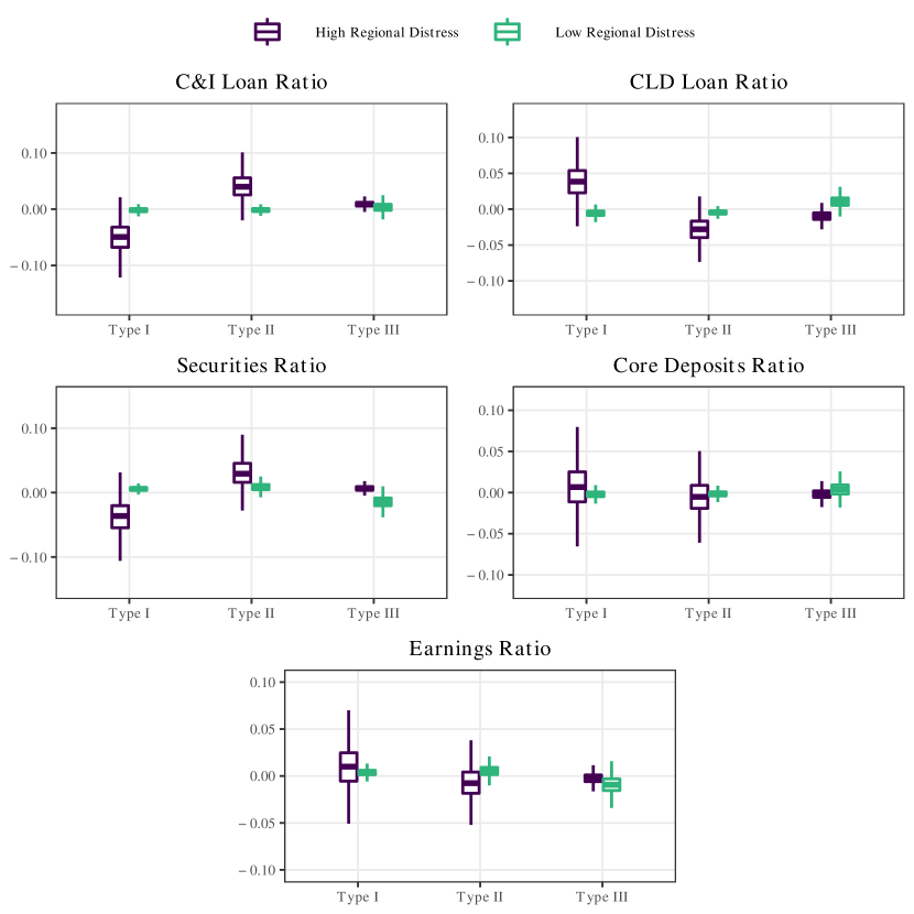
Figure 9: Additional covariate effects from the models for resolution type for banks in the class of High Regional Distress (HRD) and Low Regional Distress (LRD).

In Figure 9, a standard deviation increase in Commercial and Industrial (C&I) loan ratio is associated with an increased probability of Type II and Type III resolutions and a corresponding decline in the probability of a Type I resolution among HRD failures. These findings are consistent with the higher levels of risk attributed to increases in this ratio by the FDIC (FDIC, 1998). A standard deviation increase in Construction and Land Development Loans (CLD) is associated with an increased probability of Type I resolutions among HRD failures and of Type III resolutions among LRD failures. In the period under study, C&I loans constitute a higher concentration of bank balance sheets (27.5% of assets) than CLD loans (4.6% of assets). Accordingly, an increase in C&I loans represents a more acute concentration in that loan category and elicits a more stringent response than an equivalent increase in CLD loans.

The remaining covariates, securities ratio, core deposits ratio and earnings ratio resulted in covariate effects that were close to zero upon controlling for other balance sheet items pertaining to size, asset quality and interstate branching restrictions. An increase in each of these characteristics is associated with an increase in the bank’s franchise value and is accordingly expected to result in a lower probability of liquidation under Type III resolutions.

Appendix G Banking industry distress and FDIC’s decisions for bank resolution

We examine whether the FDIC’s responses supported Hypothesis $H_{2}$, i.e., whether the agency provided assistance with higher probability to banks that failed amid distress within the banking industry. Our results show that the agency’s decision rules qualitatively aligned with this hypothesis as it provided Type I resolutions with a marginally higher probability when the local banking industry experienced failures. However, measures of regional economic distress remained the most important determinants of membership into classes that received statistically different levels of Type I resolution.

Table 7: Covariate effects from class-membership models for specifications of latent classes based on regional and banking industry distress. The reported values are posterior means of the covariate effects. Posterior standard deviations are in parantheses.

	(5)	(6)	(7)	(8)	(9)	(10)
State-level characteristics
Unemployment	-	-	-	-0.07 (0.04)	-0.08 (0.04)	-0.1 (0.05)
County-level characteristics
Housing starts	-	-	-	0.03 (0.05)	0.04 (0.05)	0.06 (0.06)
Per capita GDP growth	-	-	-	0.04 (0.05)	0.04 (0.05)	0.07 (0.06)
Farm, agri, mining	-	-	-	0.03 (0.04)	0.04 (0.04)	0.06 (0.05)
Banking industry characteristics
Previous closures	-0.08 (0.08)	-0.07 (0.06)	-0.08 (0.07)	-0.02 (0.01)	-0.02 (0.01)	-0.01 (0.02)
% Assets in distressed banks	-0.03 (0.04)	-	-	-0.03 (0.02)	-	-
% Dep. in distressed banks	-	-0.03 (0.02)	-	-	-0.03 (0.02)	-
% distressed banks	-	-	-0.01 (0.01)	-	-	-0.02 (0.03)
Insurer characteristics
Dep. Ins. Fund/ Total Dep.	-	-	-	-0.05 (0.03)	-0.05 (0.03)	-0.05 (0.04)
log Marginal Likelihood	-719.29	-705.30	-719.14	-697.22	-697.78	-701.21

Table 7 summarizes the covariate effects and log marginal likelihood from model specifications (5) through (7) that are based purely on banking industry distress and specifications (8) through (10) that incorporate a combination of banking industry and regional economic distress. The data favor the latter three specifications over the former three as evidenced by their higher marginal likelihood. Specifically, the Bayesian model selection procedure based on posterior odds selects specification (8), which defines distress in the banking industry using previous closures and the percent of assets in distressed banks within a county. Here distressed banks are those institutions whose Texas ratio, defined in Equation (1), exceeded 100% based on previous literature that utilize this measure (Cooke et al., 2015; Siems et al., 2012). On account of the negative covariate effect of unemployment, previous closures and percent of assets in distressed banks and the positive signs for housing starts and per capita income growth, latent class 2 contains banks that failed amid relatively low regional or banking distress and banks that failed amid high regional and banking distress belong to latent class 1. As a result, in the following discussion, latent class 1 will be labeled as the class of failures under “High Regional and Banking Distress (HRBD)” and latent class 2, as the class of failures under “Low Regional and / or Banking Distress (LRBD)”.

Figure 10: Posterior distribution of the average probability of the FDIC assigning each resolution method within classes based on regional and banking distress. The horizontal axis represents the probability of assigning a resolution method and the vertical axis represents the posterior density associated with that probability based on a kernel density estimate. The solid vertical lines represent the mean of these posterior distributions across the $G$ MCMC draws.

Figure 10 provides the density of the posterior distribution of the probability of the FDIC assigning each resolution category under the selected model, specification (8). These results qualitatively align with the recommendations from Shleifer and Vishny (1992) and Acharya and Yorulmazer (2008) represented by Hypothesis $H_{2}$, which posited a greater reliance on public financial assistance in the form of Type I resolutions when the local banking industry experienced distress. The figure shows that the average probability of a Type I resolution was 26.8% under banking and regional distress and 3.5% under low regional and banking distress. These probabilities are marginally higher than the probability of Type I resolution of 24.6% and 3.3% under high and low regional distress respectively, depicted in Figure 3. Correspondingly, the average probability of Type II resolutions under banking and regional distress was 69.3%, which was lower than the equivalent probability under regional distress at 72.1%. Liquidations under Type III resolutions remained largely unchanged with probabilities of 3.9% and 3.2% respectively under classes based on high regional and banking distress and solely regional distress. The inclusion of measures of banking distress to indicators of regional distress from Section 4.1.1 primarily resulted in substitutions between Type I and II resolutions. Overall, the densities based on the two models show that measures of regional distress continue to be the most important determinants of heterogeneity in the FDIC’s decision rules and that measures of bank distress marginally augment the separation across the two classes. These findings show that banking industry distress in addition to regional distress likely contributed to a “too-many-to-fail” response from the FDIC in line with predictions from the theoretical literature (Acharya and Yorulmazer, 2007).

Appendix H Political economy factors and FDIC’s decisions for bank resolution

In this section we address constraints to the FDIC’s decision-making in the form of political pressures to provide Type I resolutions represented by Hypothesis $H_{3}$. We find that political factors played a limited role in the FDIC’s decisions as the average probability of Type I assistance to banks increased marginally from 24.6% amid economic distress to 26.5% in the presence of political support and economic distress.

The role of political economy considerations in the FDIC’s resolution decisions during the 1980’s has not been examined in detail in previous studies. The immediate reason for the sparse attention to this question in previous periods is that data on lobbying did not become available until after the Lobbying Disclosure Act of 1995. We address the paucity of data on direct measures of lobbying in two ways. First, we measure political support for financial institutions by way of the percentage of Congressional representatives from each state who voted for a bill that is favorable to the banking or S&L industry. This approach recognizes votes in favor of legislation that benefits the banking industry as indicative of lobbying efforts by the industry, which is consistent with the theoretical model of Becker (1983) in which pressure groups compete for political favors. This approach also follows from Kroszner and Strahan (1999) and Economides et al. (1996), who provide evidence of private interest groups influencing the voting behavior of elected representatives on legislation pertaining to the banking industry. Second, we include the measures of congressional voting in the class membership model that classifies banks into groups that are subject to different decision rules rather than in the model for resolution types. Consequently, instead of associating political support with the resolution method applied on specific banks, this specification suggests that such support is likely to have influenced the FDIC to adopt an overall stance that is more likely to result in assistance.

Since votes in favor of the banking industry are also likely to represent the special concerns that the elected representatives may have for the banking industry in their constituency if it is particularly distressed, measures of voting behavior potentially provide information on the condition of the industry in each state. Therefore, the classes arising from the specifications in this section represent distinct levels of “political support” instead of construing them to purely represent “regulatory capture”.

The model specifications in Table 8 consist of voting measures on bills that pertain to the regulation of the banking and S&L industry and in some cases, directly concern specific issues relating to the resolution of failed banks. The variables that measure percentage of votes in favor of a bill are based on the definition in Economides et al. (1996) and exclude representatives who did not vote. Moreover, in keeping with their specification, we also include the percentage of Republicans in each state as a covariate to ascertain that voting was not determined entirely by party affiliation. The comparison of values of log marginal likelihood reveals that the data favor specifications that include measures of regional distress over those that only generate latent classes based on political economy factors. In particular, specification (17), which has the largest marginal likelihood and thereby, the highest posterior odds relative to the remaining specifications records statistically important negative covariate effects for both state-level unemployment and the percentage of votes for the S&L restructuring bill (Bill 3). The bill to restructure the S&L industry recommended that the FDIC insure deposits held at S&L institutions in addition to commercial banks following the failure of the FSLIC. Literature on voting suggests that this bill would have elicited votes from representatives who were potentially lobbied by the beneficiaries of these bills. Institutions at risk of failure in the S&L industry would have likely benefited from and lobbied for this bill as the expanded role of the FDIC would have increased their ability to obtain assistance and function as going concerns. As a result latent class 1 will be labeled as the class of failures under “High Regional Distress and Political Support (HRDP)” and latent class 2, as the class of failures under “Low Regional Distress and / or Political Support (LRDP)”.

Table 8: Covariate effects from class-membership models for specifications of latent classes based on regional distress and political support. The reported values are posterior means of the covariate effects. Posterior standard deviations are in parantheses. The details underlying the bills in these model specifications are provided in Section A.

	(11)	(12)	(13)	(14)	(15)
State-level characteristics
Unemployment	-	-	-	-	-
Housing starts	-	-	-	-	-
County-level characteristics
Per capita GDP growth	-	-	-	-	-
Farm, agri, mining	-	-	-	-	-
Insurer characteristics
Dep. Ins. Fund/ Total Deposits	-	-	-	-	-
Political economy characteristics
% vote for Bill 4	-0.01 (0.01)	-	-	-	-
% vote for Bill 3	-	-0.02 (0.01)	-	-	-
% vote for Bill 2	-	-	0.01 (0.01)	-	-
% vote for Bill 1	-	-	-	0.01 (0.01)	-
% vote for Bill 5	-	-	-	-	0.01 (0.02)
% Republicans	0.01 (0.01)	0.02 (0.01)	0.01 (0.01)	0.01 (0)	-0.01 (0.01)
log Marginal Likelihood	-714.54	-701.29	-706.70	-716.31	-699.83
	(16)	(17)	(18)	(19)	(20)
State-level characteristics
Unemployment	-0.04 (0.02)	-0.13 (0.04)	-0.09 (0.05)	-0.1 (0.05)	-0.06 (0.03)
Housing starts	-0.06 (0.03)	-0.05 (0.04)	0.07 (0.08)	0.03 (0.09)	-0.04 (0.08)
County-level characteristics
Per capita GDP growth	-0.01 (0.03)	0 (0.04)	0.04 (0.05)	0.02 (0.05)	0.03 (0.05)
Farm, agri, mining	0.07 (0.04)	0.09 (0.05)	0.05 (0.05)	0.06 (0.04)	0.08 (0.06)
Insurer characteristics
Dep. Ins. Fund/ Total Deposits	-0.03 (0.03)	-0.05 (0.03)	-0.04 (0.04)	-0.05 (0.04)	-0.02 (0.03)
Political economy characteristics
% vote for Bill 4	-0.09 (0.02)	-	-	-	-
% vote for Bill 3	-	-0.14 (0.03)	-	-	-
% vote for Bill 2	-	-	-0.03 (0.04)	-	-
% vote for Bill 1	-	-	-	-0.05 (0.06)	-
% vote for Bill 5	-	-	-	-	0.21 (0.11)
% Republicans	0.05 (0.09)	0.12 (0.05)	0.03 (0.06)	0 (0.08)	0.2 (0.11)
log Marginal Likelihood	-698.29	-693.68	-705.50	-700.32	-704.52

Figure 11 plots the density of the posterior distribution of the average probability of the FDIC assigning each resolution method to banks in the two latent classes defined by regional distress and political economy factors in specification (17). The densities reveal that in the presence of political support to the banking industry and high regional distress, the average probability of a Type I, Type II and Type III resolution is 26.5%, 69.7% and 3.8% respectively. On comparing these average probabilities with the equivalent values of 24.6%, 72.1% and 3.2% among bank failures that occurred amid high regional distress represented in Figure 3, we find that political support for the banking industry resulted in marginally higher probability of the FDIC assigning a Type I resolution during economic distress.

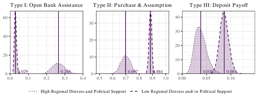
Figure 11: Posterior distribution of the average probability of the FDIC assigning each resolution method within classes based on regional distress and political economy factors. The horizontal axis represents the probability of assigning a resolution method and the vertical axis represents the posterior density associated with that probability based on a kernel density estimate. The solid vertical lines represent the mean of these posterior distributions across the $G$ MCMC draws.

The details underlying the bills in the remaining specifications are provided in Section A.

Appendix I Two Waves of Failures in the Savings and Loans Industry

The origin of distress in the S&L industry in the period of study can be traced back to events from the early 1980’s. The high interest rate regime of the late 1970’s and early 1980’s in the U.S., when the federal funds rate was set to targets as high as 20%, exposed the S&L industry to particularly severe interest rate risk owing to the regulatory constraints on these institutions. S&L institutions experienced more acute maturity mismatches than commercial banks since their liabilities, like those of commercial banks, primarily consisted of retail deposits whereas their assets were restricted to 30 year fixed rate mortgages. The rising interest expenses on deposits and the stagnated revenues from their fixed-rate mortgages led to 35.5% of S&L institutions becoming unprofitable by year-end 1980 (White, 1991).

The legislative response to distress in the S&L industry was to deregulate and provide forbearance to weak S&L’s in the form of the Depository Institutions Deregulation and Monetary Control Act of 1980 (DIDMCA) and the Garn-St Germain Depository Institutions Act of 1982. These enactments allowed S&L’s to diversify their portfolio by permitting federally chartered institutions to lend acquisition, development, and construction (ADC) loans and also authorized these institutions to offer Adjustable Rate Mortgages (ARM’s). However, these measures to ease asset-side constraints were supplemented with provisions for regulatory relief in the form of lowered net worth standards and capital requirements including even the elimination of loan-to-value restrictions on ADC loans. Effectively, these new provisions authorized S&L’s to offer a category of high-risk loans that they had no previous experience in servicing, while being required to adhere to fewer restrictions than their banking counterparts who had a longer history of offering these loans. The opportunity for high returns with lax regulatory norms resulted in an extraordinary expansion of the industry at a growth rate of 56% between 1982 and 1985(FDIC, 1998). White (1991) noted the changing composition of S&L balance sheets following these regulatory changes with traditional mortgages declining to 53% of industry assets in 1985 from their previous values of 65% in 1982 along with a material shift toward non-traditional assets such as commercial mortgage loans, land loans and direct equity investments. A second wave of failures took over the S&L industry, particularly in the Southwest and among institutions that had accumulated large shares of these non-traditional assets starting from the period 1984-1985, when both oil and real estate prices dropped precipitously and directly contributed to the deterioration of the value of projects financed by S&L institutions.

The two waves of failures in the S&L industry and the resulting regulatory response had direct implications on the the operation of the FSLIC and eventually resulted in its insolvency and dissolution in 1989. The DIDMCA increased federal deposit insurance from $40,000 to $100,000 per account (Kaufman et al., 1981), consequentially raising the FSLIC’s liabilities in the event of an S&L failure. Subsequently, the elevated levels of failure in the S&L industry depleted the resources of the FSLIC to such a dire extent that it was declared insolvent by the U.S. General Accounting Office in 1986. The Competitive Equality Banking Act of 1987 attempted to recapitalize the FSLIC by allowing it to borrow up to $10.825 billion with a cap of $3.75 billion that could be borrowed in any 12 month period. As these additional funds proved to be inadequate to resolve failed institutions, the FSLIC pursued a strategy of conducting resolutions of 222 S % L’s in 1988 with minimal cash outlays by relying on promissory notes and tax reductions for acquirers. Despite these resourceful responses, the agency was faced with 250 insolvent S&L’s with $80.8 billion in assets by the end of 1988. On February 6, 1989, President George H. W. Bush announced proposals for legislation governing the S&L industry and its regulating agencies that ultimately resulted in the Financial Institutions Reform, Recovery, and Enforcement Act (FIRREA). The proposals called for the dissolution of the Federal Savings and Loan Insurance Corporation (FSLIC) and its subsequent merger with the FDIC. The creation of the Resolution Trust Corporation (RTC) was proposed to resolve the pending cases of insolvent S&L’s. Finally, the new legislation abolished the lead agency within which the FSLIC was instituted, the Federal Home Loan Bank Board (FHLBB) that also chartered and regulated S&L’s. The Office of Thrift Supervision subsequently replaced the FHLBB in examining and supervising S&L institutions.

Appendix J Regional Distress and S&L Resolutions

In this section, we report the covariate effects of the remaining variables from the selected ordered response model in specification $3\dagger$ of Table 2. In Figure 12, across both latent classes, the probability of receiving assistance declined with a standard deviation increase in commercial and industrial (C&I) loan ratio. S&L’s, which historically specialized in retail mortgages, were permitted to lend C&I loans only in the mid-1980’s, and thereby this category represents riskier loans as S&L’s had lesser expertise and experience in evaluating these loans compared to commercial banks. Therefore, institutions with higher shares of C&I loans were less likely to be assisted and more likely to be sold to other S&L’s or liquidated. Similarly, the FSLIC was less likely to assist S&L institutions with higher shares of construction and land development (CLD) loans on their balance sheets and more likely to facilitate the acquisition of such institutions or to liquidate them. These decisions reflect the high-risk nature of CLD loans within the broader category of commercial real estate loans because projects backed by such loans may become subject to construction delays, which may result in missed loan payments. In contrast to C&I and CLD loans, S&L’s with larger shares of securities relative to total assets were more likely to be assisted and less likely to be sold or liquidated. Securities are considered to be safer and more liquid assets compared to loans, and higher shares of these assets are likely to have enabled S&L’s to retain their value through the crisis. Overall, in line with results in Figure 6, we continue to find that the FSLIC’s decision rules were homogeneous across the two latent classes.

Figure 12: Additional covariate effects from the models for resolution type for S&L’s in Regional Distress Class 1 and Regional Distress Class 2.

Appendix K S&L industry distress and FSLIC’s decisions for S&L resolution

The FSLIC’s resolution decisions do not support Hypothesis $H_{2}$. This hypothesis entails assigning the preponderance of Type I resolutions to S&L institutions that failed in the presence of distress in the S&L industry. The FSLIC did not distinguish between institutions that failed amid elevated levels of distress in the industry from those that failed in more benign industry conditions in assigning resolution decisions. As a result, the probability of the FSLIC assigning a Type I resolution was not statistically different across the two groups of S&L’s.

Table 9: Covariate effects from class-membership models for specifications of latent classes based on regional and S&L industry distress. The reported values are posterior means of the covariate effects. Posterior standard deviations are in parantheses.

	(5†)	(6†)	(7†)	(8†)	(9†)	(10†)
State-level characteristics
Unemployment	-	-	-	-0.19 (0.23)	0.06 (0.05)	0.03 (0.09)
County-level characteristics
Housing starts	-	-	-	-0.08 (0.08)	0.10 (0.07)	0.07 (0.1)
Per capita GDP growth	-	-	-	-0.10 (0.09)	0.13 (0.07)	0.17 (0.1)
Farm, agri, mining	-	-	-	-0.05 (0.07)	0.06 (0.05)	0.04 (0.05)
S&L industry characteristics
Previous closures	0.12 (0.18)	0.11 (0.18)	0.07 (0.12)	-0.03 (0.07)	0.03 (0.08)	0.03 (0.05)
% Assets in distressed S&L’s	-0.01 (0.1)	-	-	0.02 (0.07)	-	-
% Dep. in distressed S&L’s	-	-0.02 (0.09)	-	-	-0.05 (0.02)	-
% distressed S&L’s	-	-	-0.02 (0.08)	-	-	-0.09 (0.08)
Insurer characteristics
Dep. Ins. Fund/ Total Dep.	-	-	-	0.03 (0.05)	-0.03 (0.02)	-0.01 (0.06)
log Marginal Likelihood	-301.40	-300.83	-300.95	-297.15	-300.69	-300.33

Table 9 reports the covariate effects and log marginal likelihood from specifications (5^†) through (7^†) that are exclusively based on measures of distress in the S&L industry as well as from (8^†) through (10^†), which augment the specifications based on industry distress with measures of regional distress. The definition of a distressed S&L in the specifications reported in the table is an institution whose Texas ratio exceeded 100% and is consistent with the definition of distressed banks in Section G.

Bayesian model comparison identifies specification (8^†) as the selected model since it exhibits the highest marginal likelihood, and consequently the largest posterior odds relative to other specifications. However, neither the covariates pertaining to industry distress, namely, previous closures and the percentage of assets in distressed institutions, nor the measures of regional economic performance such as unemployment, housing starts and per capita income growth are statistically important in this specification. The two latent classes do not necessarily represent differences based on local economic or S&L industry characteristics. Accordingly, the two classes are labeled as “Regional and Banking Distress Class 1” and “Regional and Banking Distress Class 2”.

Figure 13: Posterior distribution of the average probability of the FSLIC assigning each resolution method within classes based on regional and S&L industry distress. The horizontal axis represents the probability of assigning a resolution method and the vertical axis represents the posterior density associated with that probability based on a kernel density estimate. The solid vertical lines represent the mean of these posterior distributions across the $G$ MCMC draws.

In Figure 13, we find that the average probability of the FSLIC assigning a Type I resolution are 69% and 76% in latent classes 1 and 2 respectively. However, the average probabilities of a Type I resolution are not statistically different across the two classes. The average probability of a Type II resolution is 25.7% in class 1 and 14.6% in class 2. Despite lesser overlap across the two densities for Type II resolutions relative to Type I resolutions, the average probabilities of the FSLIC assigning a Type II resolution are not statistically different across the two classes of S&L’s. Finally, the posterior densities of the probability of a Type III resolution entirely overlap in classes 1 and 2 with averages of 4.7% and 9.4% respectively, and are not statistically different from each other.

One of the implications of the theory from Acharya and Yorulmazer (2007, 2008) on which Hypothesis $H_{2}$ is based is that the probability of Type II resolutions are likely to be statistically different across classes of institutions that failed in high and low industry distress. According to this theoretical model, widespread distress in the S&L industry stymies the demand for failed S&L’s, which results in fewer Type II resolutions and thereby creates the necessity for assistance in the form of Type I resolutions. Since the two latent classes are not explicitly based on industry distress, the FSLIC’s resolution decisions are not consistent with this effect of S&L industry distress and thereby do not support any of the implications of Hypothesis $H_{2}$.

Appendix L Political economy factors and FSLIC’s decisions for S&L resolution

The FSLIC’s resolution decisions support Hypothesis $H_{3}$, which states that the agency was more likely to assign Type I assistance to institutions that received political support. The previous sub-sections showed that the FSLIC’s probability of assigning each resolution method did not statistically differ across groups of institutions that failed in varying levels of regional or industry distress. Among institutions that failed in the presence of political support, however, the probability of receiving a Type I resolution was statistically higher relative to institutions that failed in the absence of such support.

The specifications relating to $H_{3}$ include measures of congressional voting on bills relating to the banking and S&L industry in line with the specifications developed in Section H. The estimation of latent class models for S&L resolutions is constrained by the presence of only 15 Type III resolutions as depicted in the data summaries in Table 5 and therefore a subset of specifications are estimable. The measures of voting evaluated in this section are interpreted to represent both, lobbying by the two industries as well as the elected representatives’ concern for the health of financial institutions in their constituencies. A range of studies pertaining to the Savings and Loans crisis (Mason, 2004; Lowy, 1991) detailed the widespread lobbying efforts of both, the trade association of S&L’s viz., the U.S. League as well as individual institutions, toward influencing elected representatives on legislation that affected the regulation of the industry. However, the extent to which the FSLIC’s decisions were persuaded by such lobbying ventures has not been evaluated. We find that political economy factors played a prominent role in the decisions of the FSLIC to provide not only Type I assistance but also facilitate acquisitions and liquidate institutions under resolution Types II and III respectively.

Table 10: Covariate effects from class-membership models of S&L’s for specifications of latent classes based on regional distress and political support. The details underlying the bills in these model specifications are provided in Section A.

	($12^{\dagger}$)	($13^{\dagger}$)	($14^{\dagger}$)	($16^{\dagger}$)
State-level characteristics
Unemployment	-	-	-	-0.16 (0.13)
Housing starts	-	-	-	-0.03 (0.09)
County-level characteristics
Per capita GDP growth	-	-	-	0.13 (0.12)
Farm, agri, mining	-	-	-	0.03 (0.07)
Insurer characteristics
Dep. Ins. Fund/ Total Deposits	-	-	-	0 (0.07)
Political economy characteristics
% vote for Bill 4	-	-	-	-0.22 (0.12)
% vote for Bill 3	0.36 (0.22)	-	-	-
% vote for Bill 2	-	-0.25 (0.1)	-	-
% vote for Bill 1	-	-	-0.36 (0.09)	-
% vote for Bill 5	-	-	-	-
% Republicans	0.08 (0.15)	0.24 (0.13)	0.3 (0.09)	0.18 (0.11)
log Marginal Likelihood	-299.08	-294.01	-300.04	-301.15
	($17^{\dagger}$)	($\mathbf{18^{\dagger}}$)	($19^{\dagger}$)	($20^{\dagger}$)
State-level characteristics
Unemployment	-0.12 (0.07)	-0.03 (0.06)	-0.02 (0.06)	-0.2 (0.14)
Housing starts	0.04 (0.07)	0.03 (0.07)	0.03 (0.07)	0.01 (0.08)
County-level characteristics
Per capita GDP growth	0.06 (0.06)	0.21 (0.1)	0.08 (0.1)	0.07 (0.09)
Farm, agri, mining	-0.02 (0.04)	-0.04 (0.05)	-0.02 (0.06)	0.01 (0.05)
Insurer characteristics
Dep. Ins. Fund/ Total Deposits	-0.09 (0.06)	-0.04 (0.06)	0.03 (0.05)	0.09 (0.07)
Political economy characteristics
% vote for favor Bill 4	-	-	-	-
% vote for Bill 3	0.36 (0.11)	-	-	-
% vote for Bill 2	-	-0.14 (0.05)	-	-
% vote for Bill 1	-	-	-0.25 (0.1)	-
% vote for Bill 5	-	-	-	0.25 (0.08)
% Republicans	0.16 (0.04)	0.26 (0.08)	0.2 (0.09)	0.05 (0.08)
log Marginal Likelihood	-297.52	-288.06	-299.10	-300.40

In Table 10, the selected model is specification (18^†) by virtue of its larger marginal likelihood relative to all other specifications. This model determines latent classes based on the percent of votes in favor of a bill to reform the federal deposit insurance system and to restore civil penalties for criminal offenses involving financial institutions (Bill 2). Accordingly, votes against the bill represent political support for the S&L industry as the legislation provided for alternative mechanisms to penalize fraudulent practices by financial institutions. The covariate effects for per capita income growth, the percent vote in favor of the bill restoring civil penalties and the control for the share of Republican representatives are statistically important in the selected model. Since latent class 2 consists of institutions that failed in counties with a high per capita income growth and a low share of votes in favor of the bill, this class is labeled as “High Political Support and Low Regional Distress” and latent class 1 is the class of “Low Political Support and High Regional Distress”.

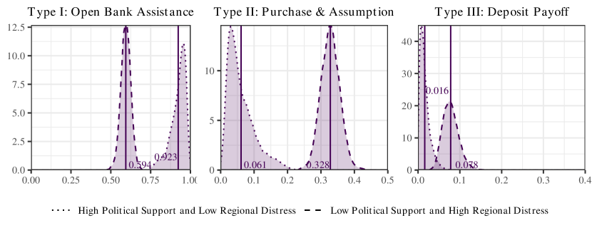
Figure 14: Posterior distribution of the average probability of the FSLIC assigning each resolution method within classes based on regional distress and political economy factors. The horizontal axis represents the probability of assigning a resolution method and the vertical axis represents the posterior density associated with that probability based on a kernel density estimate. The solid vertical lines represent the mean of these posterior distributions across the $G$ MCMC draws.

Figure 14 plots the posterior density of the probability of receiving each resolution method under specifications (18^†). Where previously, the densities in figures 5 and 13 overlapped considerably, the inclusion of measures of political support notably generates distinct latent classes with minimal overlap. This shows that the difference between the classes of S&L’s that failed in the presence of high regional distress and low political support, and those that failed in a climate of low regional distress but high degree of political support is statistically important. The FSLIC assigned Type I resolutions to institutions that failed in regions with high political support but low regional distress with average probability of 92.3% and to institutions that failed in high regional distress and low political support with a probability of 59.4%. This finding suggests that political support outweighed the effects of economic forces in determining the eligibility of failed S&L’s for assistance. The probabilities of Types II and III resolution for S&L’s that failed in the presence of political support and low levels of regional distress was 6.1% and 1.6% respectively. In the presence of regional distress and low level of political support, the FSLIC assigned Type II and III resolutions with a probability of 32.8% and 7.8% respectively. Overall, the FSLIC not only favored the assignment of assistance to institutions in regions with political support, the agency was also less likely to liquidate such institutions under Type III resolutions.

The FSLIC’s resolution decisions were more likely to have been driven by political factors as predicted by Hypothesis $H_{3}$ rather than by the extent of economic or industry distress accompanying the failure of S&L’s. Political support is measured by the share of votes in favor of legislation that affected the banking and S&L industries. Previous literature (Becker, 1983; Kroszner and Strahan, 1999; Economides et al., 1996) suggests that voting measures reveal underlying lobbying by interest groups and the potential for regulatory capture. However, in the absence of lobbying data from this period, vote shares for legislation favoring banks and S&L’s are broadly interpreted to represent the support of political representatives for these industries either due to lobbying or concerns for the health of institutions. Under either interpretation, the FSLIC deviated from hypotheses $H_{1}$ and $H_{2}$ that address moral hazard and financial stability concerns respectively and was likely influenced by motivations outside of these objectives.

References

- Acharya and Yorulmazer (2007) Acharya, V. V. and T. Yorulmazer (2007). Too many to fail - an analysis of time-inconsistency in bank closure policies. Journal of financial intermediation 16(1), 1–31.
- Acharya and Yorulmazer (2008) Acharya, V. V. and T. Yorulmazer (2008). Cash-in-the-market pricing and optimal resolution of bank failures. The Review of Financial Studies 21(6), 2705–2742.
- Akerlof et al. (1993) Akerlof, G. A., P. M. Romer, R. E. Hall, and N. G. Mankiw (1993). Looting: The economic underworld of bankruptcy for profit. Brookings papers on economic activity 1993(2), 1–73.
- Albert and Chib (1993) Albert, J. H. and S. Chib (1993). Bayesian analysis of binary and polychotomous response data. Journal of the American statistical Association 88(422), 669–679.
- Ashcraft (2005) Ashcraft, A. B. (2005). Are banks really special? new evidence from the FDIC-induced failure of healthy banks. American Economic Review 95(5), 1712.
- Balla et al. (2015) Balla, E., E. S. Prescott, and J. R. Walter (2015). Did the financial reforms of the early 1990s fail? a comparison of bank failures and FDIC losses in the 1986-92 and 2007-13 periods.
- Becker (1983) Becker, G. S. (1983). A theory of competition among pressure groups for political influence. The Quarterly Journal of Economics 98(3), 371–400.
- Bennett and Unal (2014) Bennett, R. L. and H. Unal (2014). The effects of resolution methods and industry stress on the loss on assets from bank failures. Journal of Financial Stability 15, 18–31.
- Bernanke et al. (2019) Bernanke, B. S., T. F. Geithner, and H. M. Paulson (2019). Firefighting: The financial crisis and its lessons. Penguin Books.
- Burda et al. (2008) Burda, M., M. Harding, and J. Hausman (2008). A bayesian mixed logit–probit model for multinomial choice. Journal of econometrics 147(2), 232–246.
- Chen and Dey (2000) Chen, M.-H. and D. K. Dey (2000). Bayesian analysis for correlated ordinal data models. Generalized Linear Models: A Bayesian Perspective 5, 133–158.
- Chib (1995) Chib, S. (1995). Marginal likelihood from the gibbs output. Journal of the American Statistical Association 90(432), 1313–1321.
- Chib and Jeliazkov (2001) Chib, S. and I. Jeliazkov (2001). Marginal likelihood from the metropolis–hastings output. Journal of the American Statistical Association 96(453), 270–281.
- Cooke et al. (2015) Cooke, J., C. Koch, and A. Murphy (2015). Liquidity mismatch helps predict bank failure and distress.
- Cordella and Yeyati (2003) Cordella, T. and E. L. Yeyati (2003). Bank bailouts: moral hazard vs. value effect. Journal of Financial intermediation 12(4), 300–330.
- Deb and Trivedi (1997) Deb, P. and P. K. Trivedi (1997). Demand for medical care by the elderly: a finite mixture approach. Journal of applied Econometrics 12(3), 313–336.
- DeYoung et al. (2013) DeYoung, R., M. Kowalik, and J. Reidhill (2013). A theory of failed bank resolution: Technological change and political economics. Journal of Financial Stability 9(4), 612–627.
- Duchin and Sosyura (2012) Duchin, R. and D. Sosyura (2012). The politics of government investment. Journal of Financial Economics 106(1), 24–48.
- Economides et al. (1996) Economides, N., R. G. Hubbard, and D. Palia (1996). The political economy of branching restrictions and deposit insurance: A model of monopolistic competition among small and large banks. The Journal of Law and Economics 39(2), 667–704.
- FDIC (1997) FDIC (1997). History of the Eighties: Lessons for the Future. Federal Deposit Insurance Corporation.
- FDIC (1998) FDIC (1998). Managing the Crisis: The FDIC and RTC Experience. FDIC.
- FDIC (2007) FDIC (2007). Resolutions Handbook. FDIC.
- Freixas and Rochet (2008) Freixas, X. and J.-C. Rochet (2008). Microeconomics of banking. MIT press.
- Greene et al. (2014) Greene, W., M. N. Harris, B. Hollingsworth, and P. Maitra (2014). A latent class model for obesity. Economics Letters 123(1), 1–5.
- Greene and Hensher (2003) Greene, W. H. and D. A. Hensher (2003). A latent class model for discrete choice analysis: contrasts with mixed logit. Transportation Research Part B: Methodological 37(8), 681–698.