Anunrojwong, Iyer, and Lingenbrink

Persuading Risk-Conscious Agents

Persuading Risk-Conscious Agents: A Geometric Approach

Jerry Anunrojwong Columbia Business School, jerryanunroj@gmail.com Krishnamurthy Iyer Industrial and Systems Engineering, University of Minnesota, Minneapolis, MN 55455, kriyer@umn.edu David Lingenbrink School of Operations Research and Information Engineering, Cornell University, Ithaca, NY 14853, dal299@cornell.edu

We consider a persuasion problem between a sender and a receiver whose utility may be nonlinear in her belief; we call such receivers risk-conscious. Such utility models arise when the receiver exhibits systematic biases away from expected-utility-maximization, such as uncertainty aversion (e.g., from sensitivity to the variance of the waiting time for a service). Due to this nonlinearity, the standard approach to finding the optimal persuasion mechanism using revelation principle fails. To overcome this difficulty, we use the underlying geometry of the problem to develop a convex optimization framework to find the optimal persuasion mechanism. We define the notion of full persuasion and use our framework to characterize conditions under which full persuasion can be achieved. We use our approach to study binary persuasion, where the receiver has two actions and the sender strictly prefers one of them at every state. Under a convexity assumption, we show that the binary persuasion problem reduces to a linear program, and establish a canonical set of signals where each signal either reveals the state or induces in the receiver uncertainty between two states. Finally, we discuss the broader applicability of our methods to more general contexts, and illustrate our methodology by studying information sharing of waiting times in service systems.

Revenue Management and Market Analytics Games: Bayesian persuasion, information design; Utility/preference: non-expected utility; Programming: convex optimization

1 Introduction

Given the inherent informational asymmetries in online marketplaces between a platform and its users, information design has an important role to play in their design and operation. Building on the methodological contributions of Rayo and Segal (2010), Kamenica and Gentzkow (2011), and Bergemann and Morris (2016), information design has been applied in a number of different application contexts, such as engagement/misinformation in social networks (Candogan and Drakopoulos 2020), service systems (Lingenbrink and Iyer 2019), and online retail (Lingenbrink and Iyer 2018, Drakopoulos et al. 2021).

In much of the previous work, the standard assumption is that the agent being persuaded (the receiver), is an expected utility maximizer (EUM). Although this assumption is well-supported theoretically via axiomatic characterizations (Savage 1954), it is empirically well-documented that human behavior is inadequately explained by the central tenets of the theory (Ellsberg 1961, Allais 1979, Rabin 1998, DellaVigna 2009). In particular, there is a long line of work in economics studying the systematic biases in human behavior leading to deviations from expected utility maximization (Kahneman and Tversky 1972, 1979, Machina 1982, Tversky and Kahneman 1992). Because of these shortcomings, existing models of Bayesian persuasion may not satisfactorily apply to information design problems in online markets and other practical settings.

Motivated by this concern, our main goal in this paper is to extend the methodology of Bayesian persuasion to settings where the receiver may not be an expected utility maximizer. In our general model of utility under uncertainty, given a finite state space $\Omega$ and a set of actions $A$, we take as model primitive the utility function $\rho(\mu,a)$ that specifies the receiver’s utility for action $a\in A$ under belief $\mu$. For EUM receivers, this function is given by $\rho(\mu,a)\triangleq\sum_{\omega\in\Omega}\mu(\omega)u(\omega,a)$ for some function $u$, and thus $\rho$ is linear in the belief. Our framework relaxes this linearity assumption, and allows for the utility function $\rho$ to depend non-linearly on the belief. We refer to such general receivers as risk-conscious.

Figure 1: Indifference curves in the belief space. Here, the triangle denotes the simplex of beliefs over $\Omega=\{\omega_{0},\omega_{1},\omega_{2}\}$, and the lines/curves denote the beliefs with a fixed utility. The indifference curves for EUM receivers are necessarily hyperplanes, whereas they need not be so for risk-conscious receivers.

1.1 Motivation for Risk-consciousness

While the standard model of expected utility maximization is subsumed in the risk-conscious framework, the latter allows for far more generality. Below we provide three motivation for studying risk-conscious behavior.

Deviations from EUM: The literal interpretation of risk-consciousness is that the agent’s behavior deviates systematically from expected utility maximization. Such deviations are well-documented in the literature; we provide a few examples in Table 1 and discuss them in Appendix 13. For instance, an agent with uncertainty-aversion may be modeled using mean-standard deviation utility. Thus, there is a need to develop a theory for the persuasion of such agents, both to better capture realistic behavior in operational settings and to gain qualitative insights into phenomena that do not arise with EUM receivers.

Dynamic decision making: A second source of risk-conscious behavior comes from dynamic settings where the agent must make multiple decisions over time, with past decisions influencing the information available to her in the future. For any fixed action in the present, a change in the agent’s belief may alter her actions in the future, thereby affecting her future (expected) payoffs. The net effect on the agent’s utility of a change in belief may then be non-linear, thus leading to risk-consciousness. (We provide details in Section 6.) While such models arise in a number of operational settings, a concrete example that has received recent attention is the market for data and information products (Bergemann et al. 2018, Bergemann and Bonatti 2015, 2019, Zheng and Chen 2021). A buyer in such a market often uses the data to make subsequent decisions; thus, the buyer’s utility for the data may depend non-linearly in her belief about the data quality. A seller who wishes to persuade such a buyer into purchasing the data then faces the problem of risk-conscious persuasion.

Modeling device: Finally, risk-consciousness can be a useful modeling tool to analyze more complex settings. In particular, using the risk-conscious framework, one can analyze instances of public persuasion, where a sender seeks to persuade a group of receivers by sending a common public signal; such instances are common in markets, public services, platforms, and social networks, where practical concerns such as information leakage and fairness preclude private persuasion (Candogan and Drakopoulos 2020, Candogan 2019, Yang et al. 2019, Anunrojwong et al. 2020). Similarly, the framework can be applied to study robust persuasion, where a receiver with a private type is persuaded by a sender taking a worst-case view. Robust persuasion is important in market and platform services, where participants often have idiosyncratic components to their payoffs that are unknown to the platform (Bimpikis and Papanastasiou 2019, Candogan 2020).

Table 1: Examples of risk-conscious utility

Risk-conscious utility		Utility representation $\rho(\mu,a)$
Expected utility		$\operatorname{\mathbf{E}}_{\mu}[u(\omega,a)]$
Maximin utility		$\min_{\theta}\operatorname{\mathbf{E}}_{\mu}[u(\omega,a;\theta)]$
Mean-standard deviation utility		$\operatorname{\mathbf{E}}_{\mu}[u(\omega,a)]-\beta\sqrt{\operatorname{\mathrm{Var}}_{\mu}(g(\omega,a))}$
Value-at-Risk		$-\min\{t\in\mathbb{R}:\operatorname{\mathbf{P}}_{\mu}(\ell(\omega,a)>t)\leq 1-\alpha\}$
Conditional Value-at-Risk		$-\operatorname{\mathbf{E}}_{\mu}[\ell(\omega,a)|\ell(\omega,a)>\tau]$
Cumulative prospect theory		$\sum_{\omega}f_{\omega}(\mu)u(\omega,a)$

1.2 Challenges and Opportunities

From a theoretical perspective, optimal persuasion of risk-conscious agents presents new analytical challenges. When agents are expected utility maximizers, a revelation-principle style argument is often invoked to reduce the set of possible messages the sender might send (i.e., signals) to the set of actions available to the receiver. By pairing each signal directly with the action taken by the receiver, this reduction simplifies the persuasion problem substantially, and the resulting optimization problem can be written as a linear program with one obedience constraint for each action. In contrast, with risk-conscious agents, due to the nonlinearity of the receiver’s utility, a key step of the revelation principle argument fails (as we describe in Section 3), rendering this approach to finding an optimal signaling scheme ineffective. The lack of a convenient set of signals, where each signal is paired with an optimal action, presents analytical and computational challenges to persuasion.

Despite these challenges, the setting with risk-conscious agents also yields new possibilities for persuasion. We illustrate this aspect with the following example.

Example 1.1

Consider a sender who seeks to persuade a receiver into taking an action. Let there be four payoff-relevant states $\omega\in\Omega=\{0,1,2,3\}$. The sender and the receiver’s prior belief is given by $\mu^{*}=\left(\frac{1}{4},\frac{1}{4},\frac{1}{4},\frac{1}{4}\right)$. For any belief $\mu=(\mu_{0},\mu_{1},\mu_{2},\mu_{3})$, the receiver’s utility for taking the action equals $\hat{\rho}(\mu)\triangleq\max_{\omega\in\{0,1,2\}}(\mu_{\omega}-\tfrac{2}{3})$; the receiver takes the action if and only if the utility is non-negative.

Since $\hat{\rho}(\mu^{*})<0$, without persuasion the receiver will not take the action. As $\hat{\rho}(e_{\omega})=\tfrac{1}{3}>0$ for $\omega\in\{0,1,2\}$ and $\hat{\rho}(e_{3})=-\tfrac{2}{3}<0$, under the full-information scheme that reveals the state, the receiver takes the action only in states $\omega\in\{0,1,2\}$. (Here, $e_{\omega}$ denotes the belief that puts all its weight on $\omega\in\Omega$.)

Now, consider the following signaling scheme that uses three signals $\{s_{0},s_{1},s_{2}\}$: when the state is $\omega=i\in\{0,1,2\}$, the scheme sends the signal $s_{i}$, and when the state is $\omega=3$, the scheme sends each signal with equal probability. One can verify that upon receiving the signal $s_{i}$, the receiver’s posterior belief equals $\mu^{i}=\tfrac{3}{4}e_{i}+\tfrac{1}{4}e_{3}$, with $\hat{\rho}(\mu^{i})=\tfrac{1}{12}>0$. This implies that, regardless of the signal received, the receiver finds it optimal to take the action. Thus, the preceding signaling scheme is optimal, and fully persuades the receiver into taking the action.

Note that the optimal scheme requires three signals, which is strictly more than the number of choices available to receiver. (It can be verified that under any signaling scheme that uses $2$ signals, the probability of the receiver taking the action is at most $\tfrac{3}{8}$.) This is in contrast with expected utility maximizing receivers, where the revelation principle states that action recommendations (and hence $2$ signals) suffice for optimal persuasion.

In this example, with optimal persuasion, the receiver takes the sender’s most preferred action at each state. We refer to this outcome as full persuasion, and study it in detail in Section 4. Observe that here, full persuasion occurs despite the fact that under her prior the receiver would choose otherwise. This is due to the nonlinearity inherent in the receiver’s utility, and in Theorem 4.3 we show that this cannot occur when the receiver is an expected utility maximizer.

1.3 Main Contributions

The main contributions of our paper are as follows: (1) we provide a convex optimization framework to overcome the analytical challenges in the persuasion of risk-conscious agents; (2) using this framework, we identify conditions under which persuasion is beneficial to the sender, and through the notion of full persuasion, we provide insights into the extent of this benefit; and (3) we demonstrate the structural properties of the resulting optimal persuasion mechanisms, by examining settings that impose additional regularity assumptions on the receiver’s utility.

The convex programming framework we develop in Section 3 uses the underlying geometry of the persuasion problem to optimize directly over the joint distribution of the state and the receiver’s actions. These variables are shown to lie in the convex hull of the set of beliefs for which a fixed action is optimal for the receiver. The optimal persuasion mechanism is then obtained through a convex decomposition of the optimal solution to the convex program. While related, our approach is different from the concavification approach (Kamenica and Gentzkow 2011), yielding a different convex program; we discuss the connection in detail in Appendix 8.

Using this framework, in Section 4, we first characterize conditions under which the sender strictly benefits from the persuasion of a risk-conscious receiver. This result is analogous to, and extends, similar characterization for expected-utility-maximizers (Kamenica and Gentzkow 2011). Specific to the risk-conscious framework, we formally define the notion of full persuasion as a measure of the extent of the benefits to persuasion, and provide necessary and sufficient conditions under which full persuasion is achievable.

To obtain more insight into the structure of the optimal persuasion mechanism, we then study a specialized setting in Section 5, namely binary persuasion, in which the receiver has two actions ($0$ and $1$), and the sender always prefers that the receiver choose action $1$ over action $0$. Under a convexity assumption on the receiver’s utility function, we show that the convex program in fact reduces to a linear program whose solution can be efficiently computed. By analyzing this linear program, we establish a canonical set of signals for optimal persuasion. In other words, we show there exists an optimal signaling scheme that always sends signals in this canonical set for any prior belief of the receiver. This canonical set of signals consists of pure signals, which fully reveal the state to the receiver, and binary mixed signals, which induce uncertainty between two states. With additional monotonicity assumptions on the utility function, we show that the optimal signaling scheme induces a threshold structure in the receiver’s action.

In summary, our work provides a methodology to solve for the optimal persuasion mechanism with risk-conscious agents and demonstrates the fruitfulness of analyzing more realistic models of human behavior. In Section 6, we provide a brief discussion of the use of our approach in more general settings, beyond the persuasion of a risk-conscious receiver. Finally, as an illustration of our methodology, in Section 7 we analyze a model of a queueing system where the service provider seeks to persuade arriving risk-conscious customers to join an unobservable single server queue, and establish the intricate “sandwich” structure of the optimal signaling scheme.

1.4 Literature Review

Our work contributes to the literature on Bayesian persuasion (Rayo and Segal 2010, Kamenica and Gentzkow 2011, Bergemann and Morris 2016, 2019, Taneva 2019, Kolotilin et al. 2017, Dughmi and Xu 2016), where a sender commits to a mechanism of sharing payoff-relevant information with a receiver in order to influence the latter’s actions. For a recent review of the literature, see Kamenica (2019). Our work particularly takes influence from Kamenica and Gentzkow (2011), who use a convex-analytic concavification approach to study the persuasion problem; we discuss the close relation to our work in Appendix 8.

In the operations research literature, a number of authors have applied the methodology of Bayesian persuasion to study varied settings such as crowdsourced exploration (Papanastasiou et al. 2018), spatial resource competitions (Yang et al. 2019), engagement-misinformation trade-offs in online social networks (Candogan and Drakopoulos 2020, Candogan 2019), warning policies for disaster mitigation (Alizamir et al. 2020), throughput maximization in queues (Lingenbrink and Iyer 2019), inventory/demand signaling in retail (Lingenbrink and Iyer 2018, Drakopoulos et al. 2021), and quality of matches in matching markets (Romanyuk and Smolin 2019). Our work is inspired by this stream of work, and seeks to broaden the domain of applicability by incorporating more general utility models for the receiver.

Our other source of inspiration is the economics literature on the theory of individual preferences towards risk. Apart from the standard expected utility hypothesis, there have been a number of theoretical frameworks proposed to model preferences under uncertainty, including the widely studied prospect theory (Kahneman and Tversky 1979) and the cumulative prospect theory (Tversky and Kahneman 1992). Machina (1982, 1995) singles out the “independence axiom” in the expected utility framework which leads to the utilities being “linear in the probabilities”, and study models that relax the independence axiom. Our notion of risk-consciousness encompasses all of these non-expected utility models, as it only requires the utility to be continuous in beliefs. On the other hand, our notion does not capture some non-expected utility models, such as the maxmin expected utility with multiple priors (Gilboa and Schmeidler 1989).

The notion of risk-consciousness is related to the concept of risk measures in mathematical finance (Artzner et al. 2001, Föllmer and Schied 2016). Commonly studied risk-measures, such as the variance of the portfolio return (Markowitz 1952), the value-at-risk (Jorion 2006), the expected shortfall (Acerbi and Tasche 2002), and the entropic value-at-risk (Ahmadi-Javid 2012) are all nonlinear functions of the distribution of the return. We note that to be a good measure of financial risk, a risk measure needs to satisfy a number of properties (e.g., coherence (Artzner et al. 2001)) that make sense in the context of portfolio management but may not be relevant for capturing aspects of human decision-making.

We end our discussion by mentioning two closely related recent works. Beauchêne et al. (2019) study a persuasion setting where a sender uses an ambiguous communication device comprising multiple ways of sending signals. The receiver is ambiguity-averse and has the maxmin expected utility (Gilboa and Schmeidler 1989) over the multiple resulting posteriors. As mentioned earlier, such maxmin-utility preferences are distinct from the class of risk-conscious receivers considered in this paper. The authors analyze optimal persuasion, and parallel to our result, note that full persuasion can be achieved through the use of ambiguous communication device. In contrast, our work demonstrates that full persuasion can be obtained from unambiguous communication, purely due to risk-conscious preferences.

Lipnowski and Mathevet (2018) consider persuasion of a receiver with similar nonlinear preferences as in this paper, but focus on the setting where the sender’s preferences are perfectly aligned with those of the receiver (for instance, the sender might be a trusted advisor). Noting the failure of the revelation principle, the authors provide a sufficient condition, namely that the receiver’s payoffs are concave in the belief for any fixed action, under which action recommendations are optimal. In our intended applications, the sender is a platform or a marketplace, and hence we model the sender as an expected utility maximizer. Due to this, apart from trivial instances of our model, the sender’s preferences will not be aligned with those of the receiver.

2 Model

In the following, we present the model of Bayesian persuasion with risk-conscious agents. Our development of the model follows closely to that of the standard Bayesian persuasion setting (Kamenica and Gentzkow 2011, Kamenica 2019).

2.1 Setup

We consider a persuasion problem with one sender and one receiver. Let $X$ be a payoff-relevant random variable with support on a known set $\mathcal{X}$. We assume that neither the receiver nor the sender observes $X$. However, as we describe below, the sender has more information about $X$ than the receiver, and seeks to use this information to influence the receiver’s actions.

Formally, we assume that the distribution of $X$ depends on the state of the world $\bar{\omega}$ which takes values in a finite set $\Omega$ and which is observed by the sender but not the receiver. We denote the distribution of $X$, conditional on $\bar{\omega}=\omega$, by $F_{\omega}$. The distributions $\{F_{\omega}:\omega\in\Omega\}$ are commonly known between the sender and the receiver, and both share a common prior $\mu^{*}\in\Delta(\Omega)$ about the state of the world $\bar{\omega}$. (Throughout, for any set $S$, we let $\Delta(S)$ denote the set of probability measures over $S$. When $S$ is finite, we consider $\Delta(S)$ as a subset of $\mathbb{R}^{|S|}$, endowed with the Euclidean topology.) For each $\mu\in\Delta(\Omega)$, we let $F_{\mu}$ be the distribution of $X$ when $\bar{\omega}$ is distributed as $\mu$: we have $F_{\mu}=\sum_{\omega}\mu(\omega)F_{\omega}$. Finally, we let $X_{\omega}$ denote an independent random variable distributed as $F_{\omega}$.

As in the standard Bayesian persuasion setting, we assume that the receiver is Bayesian and that the sender can commit to a signaling scheme to influence receiver’s choice of an action (which is described below in detail). A signaling scheme $(S,\pi)$ consists of a signal space $S$ and a joint distribution $\pi\in\Delta(\Omega\times S)$ such that the marginal of $\pi$ over $\Omega$ equals $\mu^{*}$: for each $\omega\in\Omega$, $\pi(\omega,S)=\mu^{*}(\omega)$. Specifically, under the signaling scheme $(S,\pi)$, if the realized state is $\bar{\omega}=\omega$, the sender draws a signal $\bar{s}\in S$ according to the conditional distribution $\pi(\cdot|\bar{\omega}=\omega)$, and conveys it to the receiver. For simplicity of notation, we denote a signaling scheme $(S,\pi)$ by the joint distribution $\pi$. Throughout, we assume that the sender commits to a signaling scheme prior to observing the state $\bar{\omega}$, and that the sender’s choice of the signaling scheme $\pi$ is common knowledge between the sender and the receiver.

As mentioned above, we assume that the receiver is Bayesian. Given the sender’s signaling scheme $\pi$, upon observing the signal $\bar{s}=s$, the receiver uses Bayes’ rule to update her belief from her prior $\mu^{*}$ to the posterior $\mu_{s}\in\Delta(\Omega)$. In particular, we have for all $\omega\in\Omega$,

$$\mu_{s}(\omega)=\frac{\pi(\omega,s)}{\sum_{\omega^{\prime}\in\Omega}\pi(\omega^{\prime},s)},$$

whenever the denominator on the right-hand side is positive. (We let $\mu_{s}\in\Delta(\Omega)$ be arbitrary if the denominator is zero.) This implies that upon receiving the signal $\bar{s}=s$, the receiver believes that the payoff-relevant variable $X$ is distributed as $F_{\mu_{s}}$.

2.2 Actions, Strategy and Utility

Upon observing the signal $\bar{s}$, the receiver chooses an action $a$ from a finite set $A$ of actions. Given a signaling scheme $\pi$, the receiver’s strategy $a(\cdot)$ specifies an action $a(s)\in A$ for each realization $s\in S$ of the signal $\bar{s}$. (Although our definition implies a pure strategy, we can easily incorporate mixed strategies where the receiver chooses an action at random. We suppress this technicality for the sake of readability.)

We let $v(\omega,a)$ denote the sender’s utility in state $\bar{\omega}=\omega$ when the receiver chooses the action $a\in A$. Furthermore, we assume that the sender is an expected utility maximizer. (One can equivalently represent the utility function $v(\omega,a)$ as an expectation of a utility function $\hat{v}(X,a)$ over the payoff-relevant variable $X$ and the action $a$, conditional on $\bar{\omega}=\omega$; we suppress the details for brevity.)

Our point of departure from the standard persuasion framework is in the definition of the receiver’s utility. Specifically, we relax the assumption that the receiver is an expected utility maximizer; as we describe next, our setup allows for more general models of the receiver’s utility over the uncertain outcome $X$. We refer to such receivers as being risk-conscious.

Formally, for any belief $\mu\in\Delta$ of the receiver, we assume that the receiver’s utility upon taking an action $a\in A$ is given by $\breve{\rho}(F_{\mu},a)\in\mathbb{R}$. For notational simplicity, we define the utility function $\rho:\Delta(\Omega)\times A\to\mathbb{R}$ as $\rho(\mu,a)\triangleq\breve{\rho}(F_{\mu},a)$. Given a belief $\mu\in\Delta(\Omega)$, we assume that the receiver chooses an action $a\in A$ that achieves the highest utility $\rho(\mu,a)$.

Observe that a receiver is an expected utility maximizer if and only if, for each $a\in A$, the utility function $\rho(\mu,a)$ is linear in $\mu$. (Note that if $\rho(\mu,a)$ is a utility function of an agent, then so is $g(\rho(\mu,a))$ for any increasing function $g:\mathbb{R}\to\mathbb{R}$. Thus, this linearity holds only up to an increasing transformation. We suppress such transformations for the sake of clarity.) In particular, there exists a function $u:\mathcal{X}\times\Omega\times A\to\mathbb{R}$ such that $\rho(\mu,a)=\operatorname{\mathbf{E}}\left[u(X,\bar{\omega},a)\right]=\sum_{\omega\in\Omega}\mu(\omega)\operatorname{\mathbf{E}}[u(X_{\omega},\omega,a)]$ for all $\mu\in\Delta(\Omega)$ and $a\in A$, if and only if the receiver is an expected utility maximizer. Our setup therefore includes as a special case the standard Bayesian persuasion framework with an expected utility maximizing receiver. However, the generality of our setting allows us to capture a much wider range of receiver behavior. (We emphasize that the notion of risk-consciousness is different from, and much more general than, the conventional notion of risk-aversion, where utility is modeled as the expectation of a function that is concave in the payoffs. A risk-averse agent is still an expected utility maximizer, and this expected utility is necessarily linear in her belief.)

From the sender’s perspective, the only relevant aspect of the receiver’s belief is the corresponding receiver’s action induced by that belief. Thus, rather than modeling receiver’s utilities directly, we could model the receiver as being characterized by the sets of beliefs for which she chooses each particular action. In other words, instead of the utility function $\rho$, our approach could equivalently take as model primitives the sets $\{\mathcal{P}_{a}:a\in A\}$, where $\mathcal{P}_{a}$ is the set of posterior beliefs for which action $a\in A$ is optimal for the receiver:

$$\mathcal{P}_{a}\triangleq\left\{\mu\in\Delta(\Omega):a\in\arg\max_{a^{\prime}\in A}\rho(\mu,a^{\prime})\right\},\quad\text{for each $a\in A$.}$$ (1)

As we discuss in Section 6, this perspective allows us to apply our methods to more general settings beyond the context of risk-conscious receivers.

As an illustration, consider the setting of a customer deciding whether or not to wait for service in an unobservable queue. The receiver’s utility depends on her unknown waiting time $X$, and suppose the queue operator observes some correlated feature $\omega$ (queue length, congestion, server availability, etc). A natural risk-conscious customer model posits that the customer only joins the queue and waits for service if, given her beliefs, the mean of her waiting time plus a multiple of its standard deviation is below a threshold (Nikolova and Stier-Moses 2014, Cominetti and Torrico 2016, Lianeas et al. 2019). Such a behavioral model may arise from the customer’s requirement for service reliability, or from an aversion to uncertainty due to a desire to plan her day subsequent to service completion. This model can be captured in our setting by letting $A=\{\mathsf{join},\mathsf{leave}\}$ and assuming, for example, that $\rho(\mu,\mathsf{join})=\tau-\left(\operatorname{\mathbf{E}}_{\mu}[X]+\beta\sqrt{\operatorname{\mathrm{Var}}_{\mu}(X)}\right)$ for some $\beta,\tau>0$, and $\rho(\mu,\mathsf{leave})=0$, implying $\mathcal{P}_{\mathsf{join}}=\left\{\mu\in\Delta(\Omega):\tau-\left(\operatorname{\mathbf{E}}_{\mu}[X]+\beta\sqrt{\operatorname{\mathrm{Var}}_{\mu}(X)}\right)\geq 0\right\}$ and $\mathcal{P}_{\mathsf{leave}}=\left\{\mu\in\Delta(\Omega):\tau-\left(\operatorname{\mathbf{E}}_{\mu}[X]+\beta\sqrt{\operatorname{\mathrm{Var}}_{\mu}(X)}\right)\leq 0\right\}$. (We use the notation $\operatorname{\mathbf{E}}_{\lambda}$ to denote expectation with respect to a distribution $\lambda$.) It is straightforward to check that $\rho(\mu,\mathsf{join})$ is not linear in $\mu$.

Throughout this paper, we make the following assumption: For each $a\in A$, the set $\mathcal{P}_{a}$ is closed. We remark that Assumption 2.2 holds if, for each $a\in A$, the utility function $\rho(\mu,a)$ is continuous in $\mu$.

2.3 Persuasion of Risk-conscious Agents

We are now ready to describe the sender’s persuasion problem. First, we require that for any choice of the signaling scheme $\pi$, the receiver’s strategy maximizes her utility with respect to her posterior beliefs: for each $s\in S$, we have

$$a(s)\in\argmax_{a\in A}\rho(\mu_{s},a).$$ (2)

We call any strategy that satisfies (2) an optimal strategy for the receiver. Given an optimal strategy $a(\cdot)$, the sender’s expected utility for choosing a signaling scheme $\pi$ is given by $\operatorname{\mathbf{E}}_{\pi}\left[v(\bar{\omega},a(\bar{s}))\right]$, where $\operatorname{\mathbf{E}}_{\pi}$ denotes the expectation over $(\bar{\omega},\bar{s})$ with respect to $\pi$. The sender seeks to choose a signaling scheme $\pi$ that maximizes her expected utility, assuming that the receiver responds with an optimal strategy. (When the receiver has multiple optimal strategies, we assume that the sender chooses her most preferred one; the literature refers to this as the sender-preferred subgame-perfect equilibrium (Kamenica and Gentzkow 2011).) Thus, the sender’s problem can be posed as

$$\max_{\pi\in\Delta(\Omega\times S)} \operatorname{\mathbf{E}}_{\pi}[v(\bar{\omega},a(\bar{s}))]$$ (3)

$$\text{subject to, }\quad a(s) \in\argmax_{a\in A}\rho(\mu_{s},a),\quad\text{for all $s\in S$,}$$

$$\pi(\omega,S) =\mu^{*}(\omega),\quad\text{for all $\omega\in\Omega$.}$$

Our main goal in this paper is to find and characterize the sender’s optimal signaling scheme to the persuasion problem (3). Note that the problem as posed is computationally challenging, as it requires first choosing an optimal set of signals $S$ and then a joint distribution $\pi$ over $\Omega\times S$. Without an explicit handle on the set $S$ and the resulting receiver actions, the persuasion problem seems intractable. In the next section, we reframe the problem to obtain a tractable formulation.

3 Towards a Tractable Formulation

When the receiver is treated as an expected utility maximizer, a revelation-principle style argument is typically invoked (Bergemann and Morris 2016) to restrict attention to signaling schemes that use the set of actions $A$ as the signaling space $S$, such that the receiver upon seeing a signal $a\in A$ finds it optimal to take action $a$. Before we discuss our approach for general risk-conscious agents, we provide a more detailed discussion of this argument, and discuss why it fails in our setting.

3.1 Failure of the Revelation Principle

The revelation-principle style argument rests on the following observation: when the receiver is an expected utility maximizer, if two signals $s_{1}$ and $s_{2}$ both lead to the same optimal action $a(s_{1})=a(s_{2})=a$, then $a$ is still an optimal action for the receiver if the signaling scheme reveals only that $\bar{s}\in\{s_{1},s_{2}\}$ whenever it was supposed to reveal $s_{1}$ or $s_{2}$. This property is straightforward to show using the linearity of the utility functions $\rho(\cdot,a)$ for an expected utility maximizer. One can then use this property to coalesce all signals that lead to the same optimal action for the receiver into a single signal. Such a coalesced signaling scheme has at most one signal per action, which after identifying the signal with the corresponding action, can be turned into an action recommendation. Moreover, for such a signaling scheme, the agent’s optimal strategy is obedient, i.e., it is optimal for the agent to follow the action recommendation.

However, when the receiver is risk-conscious, the preceding argument may no longer hold. This is because, when signals with the same optimal action are coalesced, it may alter the posterior of the receiver on the coalesced signal, and without linearity of $\rho(\cdot,a)$, the receiver’s optimal action may change. (To see this, consider Example 1.1 in reverse: under each signal $s_{i}$, it is optimal for the receiver to take the action. However, coalescing the three signals is equivalent to providing no information, and not taking the action is uniquely optimal for the receiver under her prior belief.) Thus, it no longer suffices to consider only those signaling schemes with action recommendations.

3.2 A Convex Programming Formulation

Despite this difficulty, a version of the preceding argument, which we term coalescence, continues to hold with a risk-conscious receiver. To see this, observe that if two signals $\bar{s}=s_{1}$ and $\bar{s}=s_{2}$ lead to the same posterior $\mu\in\Delta(\Omega)$ for the receiver, then the receiver’s posterior is still $\mu$ if the signaling scheme reveals only that $\bar{s}\in\{s_{1},s_{2}\}$ whenever it was supposed to reveal $s_{1}$ or $s_{2}$. This coalescence property follows immediately from the fact that the receiver’s posterior belief, given $\bar{s}\in\{s_{1},s_{2}\}$, is a convex combination of beliefs under $\bar{s}=s_{i}$ for $i=1,2$. Thus, using the same argument as before, the coalescence property allows us to coalesce all signals that lead to the same posterior belief of the receiver into a belief recommendation. In such a coalesced signaling scheme, we can take the signal space $S$ to be $\Delta(\Omega)$, the set of posteriors. Furthermore, in such a scheme, a property akin to obedience holds: if the receiver is recommended a belief $\mu$, her posterior belief is indeed $\mu$.

Summarizing the preceding discussion, we can write the sender’s persuasion problem (3) as

$$\max_{\pi\in\Delta(\Omega\times\Delta(\Omega))} \operatorname{\mathbf{E}}_{\pi}[v(\bar{\omega},a(\bar{s}))]$$ (4)

$$\text{subject to, }\quad a(s) \in\argmax_{a\in A}\rho(\mu_{s},a),\quad\text{for all $s\in\Delta(\Omega)$},$$

$$\pi(\omega,\Delta(\Omega)) =\mu^{*}(\omega),\quad\text{for each $\omega\in\Omega$,}$$

$$\mu_{s} =s,\quad\text{for all $s\in\Delta(\Omega)$}.$$

Although we have characterized the set of signals, this is still a challenging problem because of the complexity of the set $\Delta(\Omega\times\Delta(\Omega))$. To make further progress, we state the following lemma (Aumann and Maschler 1995, Kamenica and Gentzkow 2011), which gives an equivalent formulation using the notion of Bayes-plausible measures, which are probability measures $\eta\in\Delta(\Delta(\Omega))$ over the set of beliefs $\Delta(\Omega)$ with the property that their expectation equals the prior belief $\mu^{*}$. (The proof of the results in this section are in Appendix 9.)

Lemma 3.1 (Aumann and Maschler (1995), Kamenica and Gentzkow (2011))

A signaling scheme $\pi\in\Delta(\Omega\times\Delta(\Omega))$ satisfies the condition $\mu_{s}=s$ for almost all $s\in\Delta(\Omega)$, only if the measure $\eta(\cdot)\triangleq\pi(\Omega,\cdot)\in\Delta(\Delta(\Omega))$ is Bayes-plausible. Conversely, for any Bayes-plausible measure $\eta$, the signaling scheme defined as $\pi(\omega,ds)=s(\omega)\eta(ds)$ satisfies $\mu_{s}=s$ for all $s\in\Delta(\Omega)$.

The preceding lemma allows us to reformulate (4) as an optimization over the space of Bayes-plausible measures $\eta\in\Delta(\Delta(\Omega))$ with objective $\sum_{\omega\in\Omega}\operatorname{\mathbf{E}}_{\eta}\left[\bar{s}(\omega)v(\omega,a(\bar{s}))\right]$. (See Lemma 9.3 in Appendix 9 for the details.) This reformulation is still challenging, as it involves optimizing over a set of probability measures on $\Delta(\Omega)\subseteq\mathbb{R}^{|\Omega|}$. Our first result allows us to overcome this difficulty, by establishing that one can instead optimize over a much simpler space. To state our result, we need some notation: for any set $H\subseteq\mathbb{R}^{m}$, let $\mathsf{Conv}(H)$ denote the convex hull of $H$, defined as:

$$\mathsf{Conv}(H)=\left\{y:y=\sum_{i=1}^{j}\lambda_{i}x_{i},\text{for some $j\geq 1$, $\lambda_{i}\geq 0,x_{i}\in H$ for all $1\leq i\leq j$ and $\sum_{i=1}^{j}\lambda_{i}=1$}\right\}.$$

In words, $\mathsf{Conv}(H)$ is the set of all finite convex combinations of elements in $H$. We have the following lemma which states that corresponding to each Bayes-plausible measure $\eta$, there exists $\{b_{a}\geq 0\}_{a\in A}$ and $\{m_{a}\in\Delta(\Omega)\}_{a\in A}$ such that the sender’s expected utility under $\eta$, i.e., $\sum_{\omega\in\Omega}\operatorname{\mathbf{E}}_{\eta}\left[\bar{s}(\omega)v(\omega,a(\bar{s}))\right]$, can be written as a bilinear function of $m_{a}$ and $b_{a}$. Thus, the lemma allows us to directly optimize over $m_{a}$ and $b_{a}$, instead of over Bayes-plausible measures $\eta$.

Lemma 3.2

For any Bayes-plausible measure $\eta\in\Delta(\Delta(\Omega))$ and optimal receiver strategy $a(\cdot)$, there exists ${\{(b_{a},m_{a})\}}_{a\in A}$, with $b_{a}\in[0,1]$ and $m_{a}\in\mathsf{Conv}(\mathcal{P}_{a})$ for each $a\in A$, such that

$$\sum_{a\in A}b_{a}m_{a} =\mu^{*},$$ (5)

$$\operatorname{\mathbf{E}}_{\eta}\left[\bar{s}(\omega)v(\omega,a(\bar{s}))\right] =\sum_{a\in A}b_{a}m_{a}(\omega)v(\omega,a)\quad\text{for each $\omega\in\Omega$.}$$ (6)

Conversely, for any $\{(b_{a},m_{a}):b_{a}\in[0,1]\text{ and }m_{a}\in\mathsf{Conv}(\mathcal{P}_{a})\text{ for each $a\in A$}\}$ satisfying (5), there exists a Bayes-plausible measure $\eta$ and an optimal receiver strategy $a(\cdot)$ such that (6) holds.

Figure 2: In the first figure, $\eta\in\Delta(\Delta(\Omega))$ has support in the green region. Since $\eta$ is Bayes-plausible, $\operatorname{\mathbf{E}}_{\eta}[\bar{s}(\omega)]=\mu^{*}(\omega)$ for each $\omega\in\Omega$. In the second figure, we separate $\eta$ into $\eta_{0}$ and $\eta_{1}$, where $\eta_{a}$ has support in $\mathcal{P}_{a}$. In the third figure, we depict $m_{0}$ and $m_{1}$, where $\operatorname{\mathbf{E}}_{\eta_{a}}[\bar{s}(\omega)]=m_{a}^{*}(\omega)$ and $m_{a}\in\mathsf{Conv}(\mathcal{P}_{a})$. Finally, $b_{a}$ is defined as .

The interpretation of the quantities $m_{a}$ and $b_{a}$ is as follows. Given a Bayes-plausible measure $\eta$, the quantity $b_{a}$ denotes the probability that the receiver plays action $a\in A$ under the optimal strategy $a(\cdot)$, when the sender uses the signaling scheme corresponding to $\eta$; in other words, $b_{a}=$. Similarly, $m_{a}$ denotes the distribution of the state $\bar{\omega}$, conditioned on the receiver choosing action $a$. By iterated expectation, we obtain $m_{a}(\omega)=\operatorname{\mathbf{E}}_{\eta}[\bar{s}(\omega)|a(\bar{s})=a]$. Thus, for any $a\in A$, the quantity $m_{a}$ denotes the mean of all posterior beliefs the receiver holds, conditioned on her choosing action $a$. Due to this reason, we refer to $m_{a}$ as the mean-posterior of the receiver corresponding to action $a\in A$. Note that $m_{a}$ may not correspond to any actual posterior that the receiver holds when she chooses action $a\in A$; in fact, the mean-posterior $m_{a}\in\mathsf{Conv}(\mathcal{P}_{a})$ may not even lie in the set $\mathcal{P}_{a}$. Figure 2 gives some geometric intuition for these quantities, as well as for the distributions $\eta_{a}$ introduced in the proof.

While the equations (5) and (6) are bilinear in $m_{a}$ and $b_{a}$, we can make them linear by substituting $t_{a}(\omega)=b_{a}m_{a}(\omega)$ for each $\omega\in\Omega$. Notice that $b_{a}\in[0,1]$ and $m_{a}\in\mathsf{Conv}(\mathcal{P}_{a})$ imply $t_{a}\in\mathsf{Conv}(\mathcal{P}_{a}\cup\{\mathbf{0}\})$, where $\mathbf{0}\in\mathbb{R}^{|\Omega|}$ is the vector of all zeros. With this substitution, we obtain our main theorem:

Theorem 3.3

The sender’s persuasion problem (3) can be optimized by solving the following convex optimization problem:

$$\max_{\{t_{a}:a\in A\}}\ \sum_{\omega\in\Omega}\sum_{a\in A} t_{a}(\omega)v(\omega,a)$$ (7)

$$\text{subject to, }\quad\sum_{a\in A}t_{a}(\omega) =\mu^{*}(\omega),\quad\text{ for each $\omega\in\Omega$.}$$

$$t_{a} \in\mathsf{Conv}(\mathcal{P}_{a}\cup\{\mathbf{0}\}),\quad\text{ for each $a\in A$.}$$

As $m_{a}$ denotes the receiver’s mean posterior conditional on her choosing action $a$, and $b_{a}$ denotes the probability she chooses action $a$, we obtain that $t_{a}(\omega)=b_{a}m_{a}(\omega)$ denotes the joint probability that the receiver takes action $a$ and the realized state is $\bar{\omega}=\omega$. Thus, the reformulation (7) directly optimizes over the joint probability distribution of the state and the receiver’s actions.

We next briefly remark on the complexity of solving the convex program (7). First, note that relative to optimizing over Bayes-plausible measures $\eta\in\Delta(\Delta(\Omega))$, the convex program is extremely simple: the optimization is over $|A|$ variables $t_{a}$ belonging to a convex set $\mathsf{Conv}(\mathcal{P}_{a}\cup\{\mathbf{0}\})$ in $\mathbb{R}^{|\Omega|}$. Thus, its computational complexity rests on whether there exists an efficient characterization of the set $\mathsf{Conv}(\mathcal{P}_{a}\cup\{\mathbf{0}\})$ for each $a\in A$, which in turn depends solely on the properties of the utility functions $\rho(\cdot,a)$. While obtaining such an efficient characterization can be hard in general, in certain settings with additional structure on $\rho$, one can replace the convex sets $\mathsf{Conv}(\mathcal{P}_{a}\cup\{0\})$ by a convex polytope, yielding a linear program. We present and analyze one such setting in Section 5.

3.3 Optimal Signaling Schemes

To conclude this section, we describe how to get an optimal signaling scheme $\pi$ from the optimal solution $t=\{t_{a}\}_{a\in A}$ to the problem (7). Since $t_{a}\in\mathsf{Conv}(\mathcal{P}_{a}\cup\{\mathbf{0}\})$ for each $a\in A$, let $m_{a}\in\mathsf{Conv}(\mathcal{P}_{a})$ and $b_{a}\in[0,1]$ be such that $t_{a}=b_{a}m_{a}$. (Note that for $t_{a}\neq\mathbf{0}$, the corresponding $m_{a}$ is uniquely defined.) Since $m_{a}\in\mathsf{Conv}(\mathcal{P}_{a})$, there exists a finite convex decomposition of $m_{a}$ in terms of the elements of $\mathcal{P}_{a}$. That is, there exists $\{(\mu_{i}^{a},\lambda_{i}^{a}):i=1,\ldots,j_{a}\}$ for some $j_{a}\geq 1$ with $\mu^{a}_{i}\in\mathcal{P}_{a}$, $\lambda_{i}^{a}\geq 0$, and $\sum_{i}\lambda_{i}^{a}=1$, such that $m_{a}=\sum_{i=1}^{j_{a}}\lambda_{i}^{a}\mu_{i}^{a}$. An optimal signaling scheme $\pi$ is then given by the (discrete) distribution over $\Delta(\Omega\times\Delta(\Omega))$ that chooses $(\bar{\omega},\bar{s})=(\omega,\mu_{i}^{a})$ with probability $b_{a}\lambda_{i}^{a}\mu_{i}^{a}(\omega)$. Observe that conditional on $\bar{\omega}=\omega$, the optimal signaling scheme $\pi$ makes the belief recommendation $\mu_{i}^{a}$ to the receiver with probability

$$\pi(\bar{s}=\mu_{i}^{a}|\bar{\omega}=\omega) =\frac{b_{a}\lambda_{i}^{a}\mu_{i}^{a}(\omega)}{\sum_{a^{\prime}\in A}b_{a^{\prime}}\lambda_{i}^{a^{\prime}}\mu_{i}^{a^{\prime}}(\omega)}.$$ (8)

We note that in general, the representation of $m_{a}$ as a convex combination of $\mu_{i}^{a}\in\mathcal{P}_{a}$ need not be unique. Since the preceding construction works for any convex decomposition of $m_{a}$, we conclude that there may exist multiple optimal signaling schemes for the receiver.

For any set $H\subseteq\mathbb{R}^{d}$, let $\mathsf{Cara}(H)$ denote the minimum value of $j$ such that any point $x\in\mathsf{Conv}(H)$ can be written as a convex combination of at most $j$ points in $H$. The Caratheodory’s theorem (Bárány and Onn 1995) states that $\mathsf{Cara}(H)\leq\dim(H)+1$, where $\dim(H)$ is the dimension of the smallest affine space containing $H$. Thus, we obtain the following bound on the size of the set of signals the sender needs to use to optimally persuade the receiver:

Proposition 3.4

There exists an optimal signaling scheme $\pi\in\Delta(\Omega\times S)$, where the set of signals $S$ satisfies $|S|\leq\sum_{a\in A}\mathsf{Cara}(\mathcal{P}_{a})$. Specifically, for any $a\in A$, the signaling scheme sends at most $\mathsf{Cara}(\mathcal{P}_{a})\leq|\Omega|$ signals for which the receiver’s optimal action is $a$.

In the case of expected utility maximizing agents, each set $\mathcal{P}_{a}$ is convex, and hence the preceding proposition implies that at most $\mathsf{Cara}(\mathcal{P}_{a})=1$ signal per action suffices for optimal persuasion. This matches with the bound using the revelation principle, which implies the sufficiency of action recommendations. For risk-conscious receivers, the proposition states that in general, the sender must share more information than just action recommendations, and the additional information required to optimally induce any action may take up to $|\Omega|$ values.

The bound we obtain here is related to the bound obtained by Kamenica and Gentzkow (2011), who also use convex analytic arguments to show that at most $|\Omega|$ signals overall suffice for an optimal signaling scheme. In Appendix 8, we discuss this connection in detail, and use their bound to provide an alternative approach to arrive at the convex problem (7).

4 Benefits from Persuasion

Using Theorem 3.3, we now turn to the question of determining the sender’s benefits from persuasion. Let $V(\mu^{*})$ denote the optimal value of the program (7) as a function of the prior $\mu^{*}$. Similarly, let $\hat{\nu}(\mu)\triangleq\operatorname{\mathbf{E}}_{\mu}[v(\bar{\omega},a_{\mu})]$ denote the sender’s expected payoff without persuasion as a function of the prior $\mu$, where $a_{\mu}\in\{a\in A:\mu\in\mathcal{P}_{a}\}$ denotes the receiver’s optimal action under the prior.

Note that $\hat{\nu}(\mu^{*})$ is the objective value of (7) for the feasible solution $t=\{t_{a}\}_{a\in A}$ with $t_{a}=\mu^{*}$ for $a=a_{\mu^{*}}$ and $\mathbf{0}$ otherwise. Since $V(\mu^{*})$ is its optimal value, it is immediate that the sender (strictly) benefits from persuasion if and only if $V(\mu^{*})>\hat{\nu}(\mu^{*})$. The following result characterizes when the latter condition holds; the result and its proof in Appendix 10 are analogous to the setting with expected-utility maximizing receivers (Kamenica and Gentzkow 2011). Using the terminology therein, we say there is information the sender would share if there exists a belief $\mu$ with $\hat{\nu}(\mu)>\operatorname{\mathbf{E}}_{\mu}[v(\bar{\omega},a_{\mu^{*}})]$. For ease of notation, let $\mathcal{P}_{\mu}$ denote the set $\mathcal{P}_{a}$ with $a=a_{\mu}$.

Proposition 4.1

1. If there is no information the sender would share, then sender does not benefit from persuasion. If there is information sender would share, and $\mu^{*}$ lies in the interior of $\mathcal{P}_{\mu^{*}}$, then sender benefits from persuasion.

2. If for each $a\in A$ and $m_{a}\in\mathsf{Conv}(\mathcal{P}_{a})$ we have $\sum_{\omega\in\Omega}m_{a}(\omega)\left(v(\omega,a)-v(\omega,a_{\mu^{*}})\right)\leq 0$, then the sender does not benefit from persuasion. If $\mu^{*}$ is in the interior of $\mathcal{P}_{\mu^{*}}$ and there exists an $a\in A$ and an $m_{a}\in\mathsf{Conv}(\mathcal{P}_{a})$ such that $\sum_{\omega\in\Omega}m_{a}(\omega)\left(v(\omega,a)-v(\omega,a_{\mu^{*}})\right)>0$, then the sender benefits from persuasion.

The preceding result states that if the sender benefits from persuasion, then there is an action $a$ and a belief $\mu\in\mathsf{Conv}(\mathcal{P}_{a})$ such that under prior $\mu$, the sender would strictly prefer that the receiver take action $a$ over the action $a_{\mu^{*}}$. The action $a$ need not be optimal for the receiver with belief $\mu$; this is indeed the case if $\mu\in\mathsf{Conv}(\mathcal{P}_{a})\cap\mathcal{P}_{a}^{c}$. This latter scenario is impossible for an expected-utility maximizing receiver, for whom the sets $\mathcal{P}_{a}$ are convex, and hence $\mathsf{Conv}(\mathcal{P}_{a})\cap\mathcal{P}_{a}^{c}=\mathcal{P}_{a}\cap\mathcal{P}_{a}^{c}=\emptyset$.

Having obtained the conditions under which the sender benefits from persuasion, we now turn to describing the extent of this benefit. To do this, we define the notion of full persuasion that we illustrated in the introduction. Using Theorem 3.3, we will then obtain a simple characterization of when full persuasion is possible with risk-conscious receivers.

To formally define full persuasion, we start with some notations. For each action $a\in A$, let $\Upsilon_{a}\subseteq\Omega$ denote the set of pure states for which action $a$ is sender-optimal:

$$\Upsilon_{a}=\{\omega\in\Omega:v(\omega,a)\geq v(\omega,a^{\prime})\text{ for all $a^{\prime}\in A$}\}.$$

We say the sender fully persuades the receiver if there exists a signaling scheme such that at each state $\omega\in\Omega$, the receiver chooses a sender-optimal action. Formally, we have the following definition:

Definition 4.2 (Full persuasion)

A signaling scheme $\pi\in\Delta(\Omega\times S)$ fully persuades the receiver if for each $\omega\in\Omega$ and $s\in S$ with $\pi(\omega,s)>0$, if $a(s)=a$, then $\omega\in\Upsilon_{a}$. We say full persuasion is possible if there exists a signaling scheme that fully persuades the receiver.

To state the main result of this section, we make the following simplifying assumption: at each state $\omega\in\Omega$ there exists a unique action that is sender-optimal. In other words, we assume that $\{\Upsilon_{a}:a\in A\}$ forms a partition of the state space $\Omega$. For each $\omega\in\Omega$ and $a\in A$, let $t^{*}_{a}(\omega)\triangleq\mu^{*}(\omega)\mathbf{I}\{\omega\in\Upsilon_{a}\}$. We have the following theorem, whose proof is in Appendix 10:

Theorem 4.3

Suppose at each state there is a unique action that is sender-optimal. Then, the sender can fully persuade the receiver if and only if $t^{*}=(t_{a}^{*}:a\in A)$ is feasible for the convex program (7), i.e., for each $a\in A$, we have $t_{a}^{*}\in\mathsf{Conv}(\mathcal{P}_{a}\cup\{\mathbf{0}\})$.

To build intuition about the theorem, consider the scenario where there is a fixed action $a$ that is uniquely sender-optimal at all states, i.e., $\Upsilon_{a}=\Omega$ and hence, $t_{a}^{*}=\mu^{*}$. Full persuasion in this context requires the sender to persuade the receiver to always take action $a$, irrespective of the realized state. The preceding theorem implies that this is possible if and only if $\mu^{*}\in\mathsf{Conv}(\mathcal{P}_{a})$. Clearly, if $\mu^{*}\in\mathcal{P}_{a}$, the action $a$ is optimal for the receiver under the prior belief, and the receiver needs no persuasion. In other words, if $\mu^{*}\in\mathcal{P}_{a}$, the no-information scheme already fully persuades the receiver. The theorem implies that if $\mu^{*}\in\mathsf{Conv}(\mathcal{P}_{a})\cap\mathcal{P}_{a}^{c}$, there exists a signaling scheme that shares some state information and fully persuades the receiver. Once again, we note that this latter scenario cannot occur for an expected-utility maximizing receiver, for whom we have $\mathsf{Conv}(\mathcal{P}_{a})\cap\mathcal{P}_{a}^{c}=\emptyset$.

More generally, Theorem 4.3 implies that an expected-utility maximizing receiver can be fully persuaded if and only if $t_{a}^{*}$, appropriately scaled, lies in the set $\mathcal{P}_{a}$. In this case, the signaling scheme that “reveals the partition”, i.e., the scheme that at each state $\omega$ reveals the set $\Upsilon_{a}$ containing $\omega$, is sufficient to fully persuade the receiver. In contrast, for a risk-conscious receiver, the signaling scheme that fully-persuades the receiver may need to reveal more information than just revealing the partition. We explore this point in more detail in the following section.

5 Binary Persuasion

We now focus on a setting of practical importance that we refer to as binary persuasion. In this setting, the receiver’s actions are binary, i.e., $A=\{0,1\}$, and the sender’s utility is always weakly higher under action $1$, i.e., $v(\omega,1)\geq v(\omega,0)$ for all $\omega\in\Omega$. This model matches settings where, independent of the state, the sender seeks to persuade the receiver to take an action, such as engage with social media platforms (Candogan and Drakopoulos 2020), wait in a queue (Lingenbrink and Iyer 2019), or purchase a product (Lingenbrink and Iyer 2018, Drakopoulos et al. 2021).

To aid our discussion, we define the receiver’s differential utility $\hat{\rho}(\cdot)$ as the difference in the utility between choosing action $1$ and action $0$: $\hat{\rho}(\mu)\triangleq\rho(\mu,1)-\rho(\mu,0)$ for all $\mu\in\Delta(\Omega)$. Note that action $a=1$ is optimal for the receiver at belief $\mu$ if and only if $\hat{\rho}(\mu)\geq 0$.

5.1 Geometry of the Convex Program

The convex program (7) has variables defined over the domain $\mathsf{Conv}(\mathcal{P}_{a}\cup\{\mathbf{0}\})$ for each action $a$. In this section, we show that the domain can be further simplified under the following assumption: The set $\mathcal{P}_{1}^{c}=\{\mu\in\Delta(\Omega):\hat{\rho}(\mu)<0\}$ is convex.

Intuitively, the assumption implies that the receiver is averse to uncertainty when choosing action $1$: if action $1$ is not optimal under beliefs $\mu$ and $\mu^{\prime}$, then it cannot be optimal under a belief $\gamma\mu+(1-\gamma)\mu^{\prime}$ that is obtained by inducing uncertainty between $\mu$ and $\mu^{\prime}$. Furthermore, the assumption holds for a wide class of utility functions, as the following lemma establishes.

Lemma 5.1

Suppose the differential utility $\hat{\rho}(\cdot)$ is quasiconvex. Then Assumption 5.1 holds.

Specifically, Assumption 5.1 holds when $\rho(\mu,1)$ is convex and $\rho(\mu,0)$ is concave. At the same time, note that Assumption 5.1 is substantially weaker than requiring quasiconvexity of $\hat{\rho}$, since the latter implies that every level set $\{\mu:\hat{\rho}(\mu)<c\}$ is convex.

Using Assumption 5.1, we now show that the convex program (7) can be simplified to a linear program. Recall that $e_{\omega}$ denotes the belief that assigns all its weight to $\omega\in\Omega$. By a slight abuse of notation, we identify $\omega\in\Omega$ with $e_{\omega}$ and consider $\Omega$ as a subset of $\Delta(\Omega)$.

Let $K_{1}\triangleq\mathcal{P}_{1}\cap\Omega$ denote the set of states where action $1$ is optimal for the receiver under full-information. Similarly, let $K_{0}\triangleq\mathcal{P}_{0}\cap\Omega$ be the set of states where action $0$ is optimal for the receiver under full-information. Note, $K_{0}\cap K_{1}$ may be non-empty if the receiver finds both actions optimal at some state. We let $L_{0}\triangleq K_{0}\cap K_{1}^{c}$ denote the set of states for which action $0$ is uniquely optimal for the receiver.

Next, for $\omega_{0}\in L_{0}$ and $\omega_{1}\in K_{1}$, consider the set of beliefs obtained as the convex combination of $\omega_{0}$ and $\omega_{1}$. In this set, we let $\chi(\omega_{0},\omega_{1})$ denote the belief that puts the largest weight on $\omega_{0}$ while still preserving the optimality of action $1$ for the receiver. (Since $\mathcal{P}_{1}$ is closed, such a maximal convex combination exists.) Formally, for $\omega_{0}\in L_{0}$ and $\omega_{1}\in K_{1}$, we define $\gamma(\omega_{0},\omega_{1})=\sup_{\gamma\in[0,1]}\left\{\gamma:\gamma\omega_{0}+(1-\gamma)\omega_{1}\in\mathcal{P}_{1}\right\}$, and let $\chi(\omega_{0},\omega_{1})=\gamma(\omega_{0},\omega_{1})\omega_{0}+(1-\gamma(\omega_{0},\omega_{1}))\omega_{1}$. Since $\mathcal{P}_{0}$ and $\mathcal{P}_{1}$ are closed, we obtain that $\chi(\omega_{0},\omega_{1})\in\mathcal{P}_{0}\cap\mathcal{P}_{1}$, and hence the receiver is indifferent between action $0$ and $1$ at belief $\chi(\omega_{0},\omega_{1})$. Finally, we define the set $K_{01}$ to be a subset of such maximal convex combinations $\chi(\omega_{0},\omega_{1})$:

$$K_{01}=\{\chi(\omega_{0},\omega_{1})\in\Delta(\Omega)\text{ for some $\omega_{0}\in L_{0}$ and $\omega_{1}\in K_{1}$}\}.$$ (9)

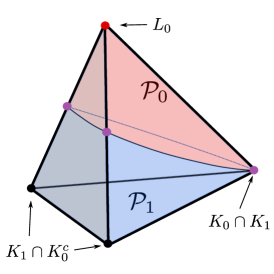
Figure 6: The sets $L_{0},K_{0}$ and $K_{1}$ when $K_{0}\neq L_{0}$. Here, $K_{01}$ is the set of the purple vertices.

We note that while $K_{01}\cap L_{0}$ must be empty, the sets $K_{01}\cap K_{0}$ and $K_{01}\cap K_{1}$ can be non-empty. We illustrate these sets pictorially in Fig. 3 (and in Fig. 6 in Appendix 11).

(a) The set $K_{0}=\Omega\cap\mathcal{P}_{0}$.

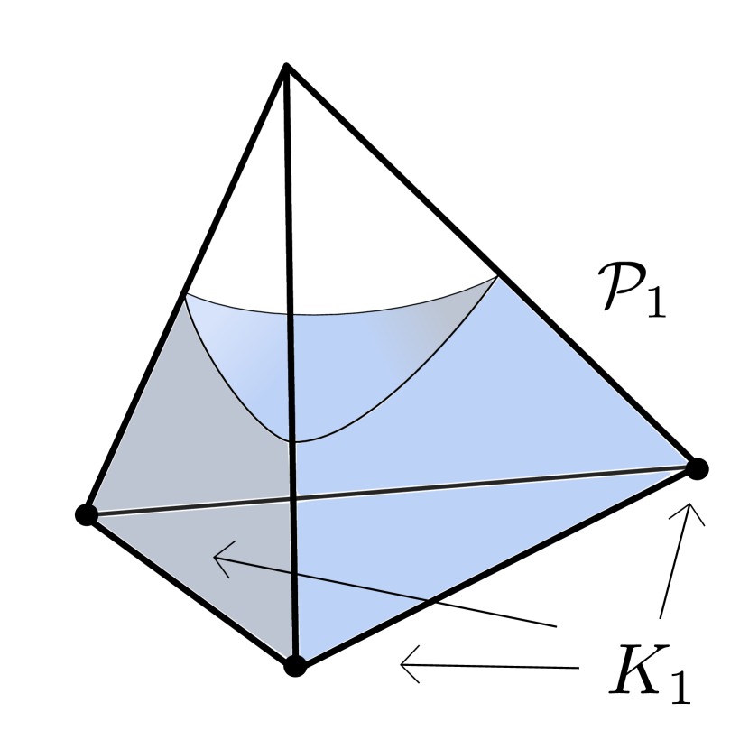
(b) The set $K_{1}=\Omega\cap\mathcal{P}_{1}$.

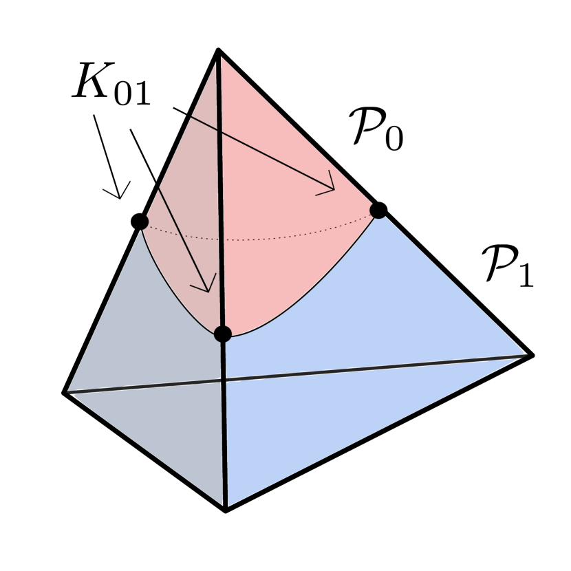
(c) The set $K_{01}$ as defined in (9).

Figure 3: The sets $K_{0},K_{1}$ and $K_{01}$. (Here, the red region is the set $\mathcal{P}_{0}$ and the blue region is $\mathcal{P}_{1}$. Furthermore, in this example, $L_{0}=K_{0}$.)

With these definitions, we can state the main theorem of this section. The full proof is provided in Appendix 11.

Theorem 5.2

Under Assumption 5.1, the sender’s persuasion problem (7) can be optimized by solving the following linear program:

$$\begin{aligned} \max_{t_{0},t_{1}}&\sum_{\omega\in\Omega}v(\omega,1)t_{1}(\omega)+v(\omega,0)t_{0}(\omega)\\ \text{subject to,}\quad t_{1}&\in\mathsf{Conv}(K_{1}\cup K_{01}\cup\{\mathbf{0}\}),\\ t_{0}&\in\mathsf{Conv}(L_{0}\cup\{\mathbf{0}\}),\\ t_{0}(\omega)+t_{1}(\omega)&=\mu^{*}(\omega)\quad\text{for each }\omega\in\Omega.\end{aligned}$$ (10)

The proof intuition is as follows. First, under Assumption 5.1, we prove in Lemma 11.4 that the set $\mathsf{Conv}(\mathcal{P}_{1})$ is a convex polytope with extreme points in $K_{1}\cup K_{01}$, and hence the constraint $t_{1}\in\mathsf{Conv}(\mathcal{P}_{1}\cup\{\mathbf{0}\})$ in (7) is equivalent to the constraint $t_{1}\in\mathsf{Conv}(K_{1}\cup K_{01}\cup\{\mathbf{0}\})$. Second, we establish that any $t_{0}\in\mathsf{Conv}(\mathcal{P}_{0}\cup\{\mathbf{0}\})$ that is not in $\mathsf{Conv}(L_{0}\cup\{\mathbf{0}\})$ cannot be part of an optimal solution, by improving on any such feasible solution. See Fig. 4 (and Fig. 7 in Appendix 11) for some geometric intuition.

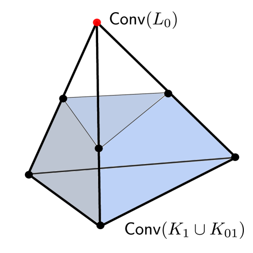
Figure 4: Geometry of $\mathsf{Conv}(L_{0})$ and $\mathsf{Conv}(K_{1}\cup K_{01})$. Here, $\mathsf{Conv}(L_{0})$ is the red vertex of the simplex.

5.2 Structural Characterizations

The preceding theorem implies several results about the structure of the optimal signaling scheme.

First, Theorem 5.2 establishes a canonical set of signals for an optimal signaling scheme, namely the set $\Omega\cup K_{01}$. In other words, for a given binary persuasion setting, irrespective of the prior belief $\mu^{*}$, it suffices to only send signals in the set $\Omega\cup K_{01}$. This follows from the fact that Theorem 5.2 implies that the mean-posteriors $m_{0}$ and $m_{1}$ satisfy $m_{0}\in\mathsf{Conv}(L_{0})$ and $m_{1}\in\mathsf{Conv}(K_{1}\cup K_{01})$. Hence, $m_{0}$ can be expressed as a convex combination of beliefs in $L_{0}$, and $m_{1}$ can be expressed as a convex combination of beliefs in $K_{1}\cup K_{01}$. Thus, it follows that inducing beliefs in the set $L_{0}\cup K_{1}\cup K_{01}=\Omega\cup K_{01}$ suffices for optimal persuasion.

Second, observe that the canonical set consists of pure signals $\omega\in\Omega$ which fully reveal the state $\omega$, and binary mixed signals $\chi(\omega_{0},\omega_{1})\in K_{01}$ which induce a belief over two states $\omega_{0}\in L_{0}$ and $\omega_{1}\in K_{1}$. Thus, the optimal persuasion can always be achieved by either fully revealing the state, or making the receiver uncertain about two states. Of course, due to the convexity of $\mathcal{P}_{1}^{c}$, there also exists an optimal signaling scheme where all posteriors that lead to the receiver taking action $0$ are replaced with a single action recommendation “take action $0$”.

Note that since $t_{0}\in\mathsf{Conv}(L_{0}\cup\{\mathbf{0}\})$, if the optimal signaling scheme induces the sender’s least-preferred action $0$, then the receiver’s belief only puts weight on states in the set $L_{0}$. At each of these states, the action $0$ is uniquely optimal for the receiver. This is analogous to a similar structural result for expected-utility maximizing receivers (Kamenica and Gentzkow 2011, Proposition 4).

In the setting of binary persuasion, our earlier results regarding full persuasion simplify and yield a simple condition to determine if the receiver can be fully persuaded. Suppose at all states, the sender strictly prefers action $1$. Then, using the notation of Section 4, we have $\Upsilon_{1}=\Omega$, and thus Theorem 4.3 implies that the receiver can be fully persuaded if and only if $\mu^{*}\in\mathsf{Conv}(\mathcal{P}_{1})$. As we prove in Lemma 11.4, under Assumption 5.1, we have $\mathsf{Conv}(\mathcal{P}_{1})=\mathsf{Conv}(K_{1}\cup K_{01})$. Thus we obtain a simple criterion, namely whether $\mu^{*}\in\mathsf{Conv}(K_{1}\cup K_{01})$, to determine if full persuasion is possible.

Finally, the linear programming formulation allows us to further characterize the structure of the optimal signaling scheme when the differential utility function $\hat{\rho}$ satisfies a monotonicity condition. For simplicity, we focus on the case where $v(\omega,1)-v(\omega,0)=v>0$ for all $\omega\in\Omega$. We consider the following condition on the differential utility function: [Monotonicity] There exists a strict total order $\prec$ on $\Omega$ such that if $\omega\prec\omega^{\prime}$, then either (1) $\omega\in K_{1}$ or (2) $\omega,\omega^{\prime}\in L_{0}$ and $\gamma(\omega,\hat{\omega})>\gamma(\omega^{\prime},\hat{\omega})$ for all $\hat{\omega}\in K_{1}$.

Recall that for $\omega_{0}\in L_{0}$ and $\omega_{1}\in K_{1}$, $\gamma(\omega_{0},\omega_{1})$ is the largest value of $\gamma\in[0,1]$ such that the belief $\gamma\omega_{0}+(1-\gamma)\omega_{1}$ lies in $\mathcal{P}_{1}$. Thus, the preceding monotonicity condition implies that for any $\omega,\omega^{\prime}\in L_{0}$ with $\omega\prec\omega^{\prime}$ and for any $\omega_{1}\in K_{1}$, if $\gamma\omega^{\prime}+(1-\gamma)\omega_{1}$ lies in $\mathcal{P}_{1}$, then so does $\gamma\omega+(1-\gamma)\omega_{1}$.

A wide class of differential utility functions satisfies monotonicity, including the class of expected utility functions. In particular, given a strict total order on $\Omega$, the condition holds for any differential utility function $\hat{\rho}(\cdot)$ that is strictly decreasing under the first-order stochastic ordering on $\mu$.

We have the following result with proof in Appendix 11:

Proposition 5.3

Suppose $v(\omega,1)-v(\omega,0)=v>0$ for all $\omega\in\Omega$, and the differential utility function $\hat{\rho}$ satisfies Assumptions 5.1 and 5.2. Then the optimal signaling scheme induces a threshold structure in the receiver’s actions: there exists an $\omega_{0}\in L_{0}$ such that

$$t_{1}(\omega) =\begin{cases}\mu^{*}(\omega)&\text{ if $\omega\prec\omega_{0}$;}\\ 0&\text{if $\omega_{0}\prec\omega$.}\end{cases}$$

In particular, under the optimal signaling scheme, the receiver chooses action $1$ in states $\omega\prec\omega_{0}$, and chooses action $0$ in states $\omega$ with $\omega_{0}\prec\omega$.

Finally, we emphasize that it is the induced action of the receiver that has a threshold structure; the optimal signaling scheme typically possesses a more intricate structure in order to induce beliefs in $\Omega\cup K_{01}$. (We illustrate this structure in more detail in an application in Section 7.)

6 Broader Applicability to other Contexts

Next, we discuss the broader applicability of our approach to more general contexts beyond the literal interpretation of persuading risk-conscious receivers.

As mentioned in the introduction, risk-consciousness arises naturally in dynamic decision-making settings even with expected-utility-maximizers. To illustrate, consider a two-period setting where the receiver, after choosing an action $a\in A$ in the first period, must choose an action $d\in D$ in the second period. After taking the first-period action $a$ but prior to the choice of $d$, the receiver obtains additional state information whose quality depends on the choice of the first-period action. Formally, the receiver observes the realization of a random variable $Z$ whose distribution depends on $(\omega,a)$. A natural model of utility that captures this setting is given by

$$\rho(\mu,a)\triangleq\operatorname{\mathbf{E}}_{\mu}\left[u(\omega,a)+\max_{d\in D}\operatorname{\mathbf{E}}_{\mu}\left[r_{a}(\omega,d)\big{|}Z,a\right]\right],$$

where $u(\omega,a)$ is the receiver’s first-period utility, and $r_{a}(\omega,d)$ denotes her utility in the second-period. Letting $d_{\mu}(Z,a)$ denote the decision rule that attains the inner maximization, the receiver’s utility can be written as $\rho(\mu,a)=\operatorname{\mathbf{E}}_{\mu}\left[u(\omega,a)+r_{a}(\omega,d_{\mu}(Z,a))\right]$. It follows that, in general, $\rho(\mu,a)$ is non-linear in $\mu$. A special case of this general model arises in data markets, where a buyer must choose whether to purchase relevant data ($a=1$) or not ($a=0$) before making a decision (Bergemann et al. 2018, Bergemann and Bonatti 2015, 2019, Zheng and Chen 2021). Letting $Z$ denote the information content of the data, we have $\rho(\mu,0)=\max_{d\in D}\operatorname{\mathbf{E}}_{\mu}[r_{0}(\omega,d)]$ and $\rho(\mu,1)=\operatorname{\mathbf{E}}_{\mu}\left[\max_{d\in D}\operatorname{\mathbf{E}}_{\mu}[r_{1}(\omega,d)|Z]\right]$. In such setting, a seller who wishes to persuade the buyer to purchase the data faces the problem of persuading a risk-conscious receiver.

Our methods can be used to study public persuasion (Arieli and Babichenko 2019, Yang et al. 2019, Das et al. 2017, Candogan and Drakopoulos 2020, Bimpikis et al. 2019) of a group of interacting agents, where the sender shares information publicly with all the agents. For any public signal, the agents share a common posterior and subsequently play an equilibrium of an incomplete information game. The sender seeks to publicly share payoff-relevant information to influence the agents’ choice of the equilibrium. To apply our methods, we view the group of agents as a single risk-conscious receiver, and the equilibrium profile as the action chosen by the receiver. Then, for any equilibrium $a$, the set $\mathcal{P}_{a}$ describes the set of common posteriors for which the agents play the same equilibrium profile $a$. With this mapping, our results can be used to find the optimal public signaling scheme, as long as the set of (relevant) equilibria over all common posteriors is finite (see, e.g., (Yang et al. 2019)).

Another application of our methods is to robust persuasion (Hu and Weng 2021, Inostroza and Pavan 2021, Ziegler 2020), where a sender persuades a single receiver with a private type $\theta\in\Theta$. The sender takes a worst-case view, and seeks to persuade the receiver irrespective of her type. Formally, suppose the utility of the type-$\theta$ receiver with belief $\mu$ for action $a$ is given by $\rho_{\theta}(\mu,a)$, and let $a_{\theta}(\mu)\in\arg\max_{a}\rho_{\theta}(\mu,a)$ denote the optimal action chosen by the receiver. Let $v(a)$ denote the sender’s (state-independent) utility when the receiver chooses action $a$. Since the receiver’s type $\theta$ is unknown to the sender, she maximizes the (expectation) of the minimum of her utility across all receiver types: $\operatorname{\mathbf{E}}[\min_{\theta}v(a_{\theta}(\mu_{s}))]$. Here, $\mu_{s}$ is the receiver’s posterior belief subsequent to persuasion. Such a setting of robust persuasion maps to our model, with the sets $\mathcal{P}_{a}$ given by $\mathcal{P}_{a}=\{\mu\in\Delta(\Omega):v(a)=\min_{\theta}v(a_{\theta}(\mu))\}$ for each $a\in A$. Thus, our results yield a robust signaling scheme through a convex program.

7 Application: Signaling in Unobservable Queues

We conclude the paper with an illustrative application of our methodology to study information sharing in a service system where arriving customers must choose whether or not to join an unobservable queue to obtain service. The model is based on that of Lingenbrink and Iyer (2019), with the difference being that here customers are not expected utility maximizers. Instead, inspired by the literature on the psychology of waiting in queues (Maister 1984), we consider customers who exhibit uncertainty aversion. Formally, the customers have a mean-standard deviation utility (Nikolova and Stier-Moses 2014, Cominetti and Torrico 2016, Lianeas et al. 2019), where the disutility for joining the queue is the sum of the mean waiting time and a multiple of its standard deviation. Moreover, the setting has a key difference from the model in Section 2: the customers’ (receiver’s) prior belief is endogenously determined from the equilibrium queue dynamics. We show that our theoretical results carry over to this setting, and establish that the optimal signaling scheme has an intricate “sandwich” structure.

We consider a service system modeled as an unobservable $M/M/1/C$ FIFO queue, i.e. a single-server queue with Poisson arrivals with rate $\lambda$, independent exponential service times with unit mean, and queue capacity $C>0$. Upon arrival, each customer chooses whether to join the queue to receive service ($a=1$) or leave without obtaining service ($a=0$); a customer cannot join the queue if there are $C$ customers already in queue. We assume that customers are averse to waiting, but cannot observe the queue length before making joining decision. Instead, the service provider can observe the queue length and communicate this information to arriving customers. The service provider aims to maximize the queue throughput; if service is offered at a fixed price, this translates to maximizing the revenue rate.

As the customer cannot join the queue if the queue length is $C$, the relevant state space is $\Omega=\{0,1,\ldots,C-1\}$, where the state $\bar{\omega}\in\Omega$ describes the queue length upon a customer arrival. To focus on throughput-maximization, we set $v(\omega,a)=a$ for $\omega\in\Omega$ and $a\in\{0,1\}$.

For an arriving customer, the payoff-relevant variable $X$ is their waiting time until service completion. When $\bar{\omega}=n\in\Omega$, the waiting time $X$ is distributed as the sum of $n+1$ independent unit exponentials (the waiting times for $n$ customers in the queue plus the customer’s own service time). To capture uncertainty aversion on the part of the customers (Maister 1984), we focus on the following differential utility function for joining the queue:

$$\hat{\rho}(\mu)\triangleq\tau-\left(\operatorname{\mathbf{E}}_{\mu}[X]+\beta\sqrt{\operatorname{\mathrm{Var}}_{\mu}[X]}\right),$$ (11)

where $\mu\in\Delta(\Omega)$ is the customer’s belief about the queue length, $\tau>0$ captures her value for service, and $\beta\geq 0$ captures her degree of risk-consciousness. It is straightforward to verify that $\hat{\rho}(\cdot)$ satisfies convexity (Assumption 5.1) and monotonicity (Assumption 5.2); see Appendix 12 for the details.

Using the results from Section 5 and the same approach as in Lingenbrink and Iyer (2019) to handle endogenous priors, we obtain that the service provider’s signaling problem can be optimized by solving the following linear program:

$$\max_{t_{0},t_{1}}\sum_{\omega\in\Omega}t_{1}(\omega)$$

subject to, $$t_{1}\in\mathsf{Conv}(K_{1}\cup K_{01}\cup\{\mathbf{0}\}),$$ (12a)

$$t_{0}\in\mathsf{Conv}(L_{0}\cup\{\mathbf{0}\}),$$ (12b)

$$t_{0}(\omega+1)+t_{1}(\omega+1)=\lambda t_{1}(\omega),\quad\text{ for each $\omega<C-1$,}$$ (12c)

$$\sum_{\omega\in\Omega}t_{0}(\omega)+\sum_{\omega\in\Omega}t_{1}(\omega)+\lambda t_{1}(C-1)=1.$$ (12d)

Here, the objective captures the probability that an arriving customer joins the queue, whereas the constraint (12c) captures the detailed-balance conditions on the steady-state distribution of the queue. The constraint (12d) is the normalization condition for the steady-state distribution (with $\lambda_{1}t_{1}(C-1)$ being the probability that the queue is at capacity).

Using the monotonicity of the differential utility function, our first result shows the optimal signaling scheme induces a threshold structure on the customers’ actions. The proof uses a perturbation argument similar to Lingenbrink and Iyer (2019), and is presented in Appendix 12.1.

Lemma 7.1

An optimal signaling scheme induces a threshold structure in the customers’ actions: there exists an $m\in\Omega$ such that an arriving customer joins the queue if the queue length is strictly less than $m$ and leaves if it is strictly greater than $m$.

While the preceding lemma provides insights into the structure of the customers’ actions, it does not reveal the structure of an optimal signaling scheme. The following main result of this section characterizes the intricate structure of an optimal signaling scheme using the canonical set of signals (as described in Section 5). The proof is given in Appendix 12.2.

Proposition 7.2

Suppose the optimal solution $t=(t_{0},t_{1})$ to (12) satisfies $t_{0}\neq\mathbf{0}$. Then, there exists an optimal signaling scheme with signals $S=\{\mathsf{Join}_{1},\mathsf{Join}_{2},\ldots,\mathsf{Join}_{J},\mathsf{Leave}\}$ for some $J\leq|\Omega|$, such that joining the queue is optimal under each signal $\mathsf{Join}_{j}$, and leaving is optimal under the signal $\mathsf{Leave}$. Furthermore,

1. For each $j\leq J$, a customer’s utility upon receiving the signal $\mathsf{Join}_{j}$ is zero, i.e., $\hat{\rho}(\mu_{j})=0$, where $\mu_{j}$ is the induced belief upon receiving signal $\mathsf{Join}_{j}$.

2. For each $j\leq J$, the induced belief $\mu_{j}$ either puts all its weight on a state $\omega^{j}\in K_{1}\cap K_{0}$, or there exists two states $\omega_{0}^{j}\in L_{0}$ and $\omega_{1}^{j}\in K_{1}$ such that $\mu_{j}$ puts positive weight only on the states $\omega_{0}^{j}$ and $\omega_{1}^{j}$. (In the former case, we define $\omega_{0}^{j}=\omega_{1}^{j}=\omega^{j}$.) These states form a sandwich structure: $\omega_{1}^{1}\leq\omega_{1}^{2}\leq\cdots\leq\omega_{1}^{J}\leq\omega_{0}^{J}\leq\omega_{0}^{J-1}\leq\cdots\leq\omega_{0}^{1}$.

3. For each $j\leq J$, we have $\operatorname{\mathbf{E}}[X|\mathsf{Join}_{j-1}]\leq\operatorname{\mathbf{E}}[X|\mathsf{Join}_{j}]$ and $\operatorname{\mathrm{Var}}(X|\mathsf{Join}_{j-1})\geq\operatorname{\mathrm{Var}}(X|\mathsf{Join}_{j})$.

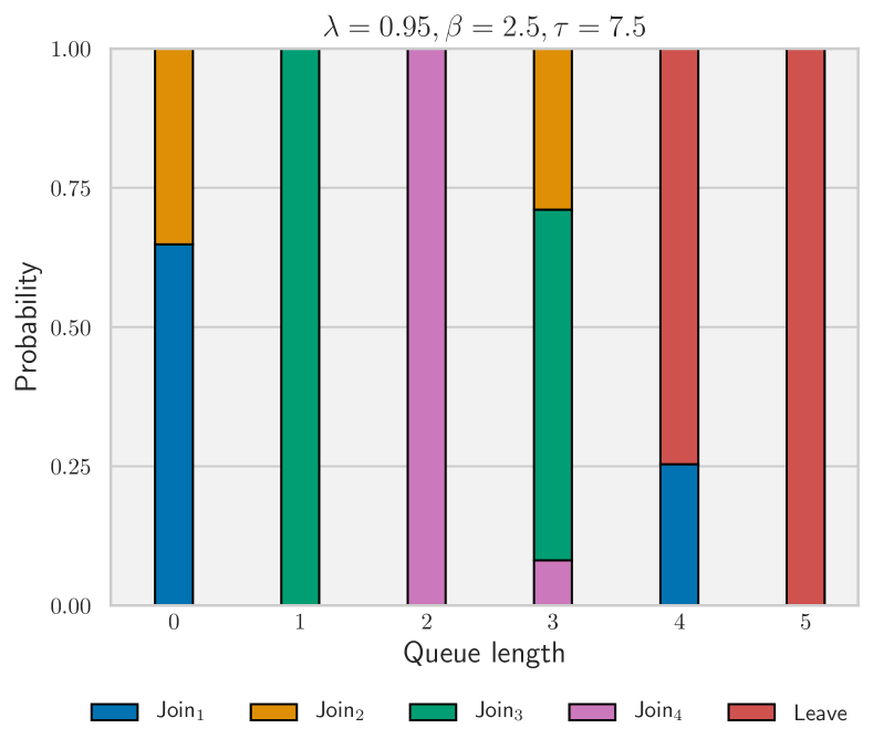
Signal $s$		Posterior belief		$\operatorname{\mathbf{E}}[X|s]$
$\mathsf{Join}_{1}$		$0.76\cdot e_{0}+0.24\cdot e_{4}$		1.97
$\mathsf{Join}_{2}$		$0.59\cdot e_{0}+0.41\cdot e_{3}$		2.24
$\mathsf{Join}_{3}$		$0.64\cdot e_{1}+0.36\cdot e_{3}$		2.72
$\mathsf{Join}_{4}$		$0.93\cdot e_{2}+0.07\cdot e_{3}$		3.07
$\mathsf{Leave}$		$0.76\cdot e_{4}+0.24\cdot e_{5}$		5.24

Figure 5: Optimal signaling schemes

The preceding proposition states implies that, assuming not all customers join the queue, the customer’s utility upon receiving any $\mathsf{Join}_{j}$ signal is zero, and hence $\operatorname{\mathbf{E}}_{\mu}[X|\mathsf{Join}_{j}]+\beta\sqrt{\operatorname{\mathrm{Var}}_{\mu}[X|\mathsf{Join}_{j}]}=\tau$ for all $j\leq J$. Thus, the optimal signaling mechanism compensates for the higher expected waiting times under some signals with lower variance, leading to the sandwich structure in the induced posterior beliefs.

We numerically illustrate the preceding result in Figure 5, for $(\lambda,\beta,\tau)=(0.95,2.5,7.5)$ and $C=100$. We depict an optimal signaling scheme that uses $5$ signals ($\mathsf{Join}_{1}$, $\mathsf{Join}_{2}$, $\mathsf{Join}_{3}$, $\mathsf{Join}_{4}$ and $\mathsf{Leave}$), the first four of which persuade the customer to join. The plot on the left shows the probabilities of sending each signal conditional on the queue length. For instance, if the queue length is $\omega=3$ upon a customer arrival, the signals $\mathsf{Join}_{2}$, $\mathsf{Join}_{3}$, $\mathsf{Join}_{4}$ are sent with probabilities $0.29$, $0.63$, and $0.08$, respectively. As established in Lemma 7.1, the plot reveals the threshold structure induced on the customers’ actions: a customer joins for queue lengths smaller than $4$, and leaves for queue lengths larger than $4$. The table on the right shows the induced posterior belief upon receiving each signal. We see that each signal $\mathsf{Join}_{j}$ puts weight only on two states and these states form a sandwich structure. The sandwich structure also orders the signals in the increasing order of mean waiting times; since the customer’s differential utility upon receiving any $\mathsf{Join}_{j}$ signal is zero, the variance of the waiting time is decreasing. This ordering provides a convenient vocabulary for the service provider to communicate with the customers: rather than sending an abstract signal such as $\mathsf{Join}_{j}$, the service provider can directly convey the induced expected waiting times $\operatorname{\mathbf{E}}[X|\mathsf{Join}_{j}]$ (or the induced uncertainty $\sqrt{\operatorname{\mathrm{Var}}(X|\mathsf{Join}_{j})}$).

8 Relation to the Concavification Approach

In their seminal work, Kamenica and Gentzkow (2011) (hereafter [KG11]) present a convex analytic concavification approach to find the optimal signaling scheme in persuasion problems. Furthermore, in Proposition 4 of the online appendix of [KG11], the authors establish that the number of signals in an optimal signaling scheme can be upper-bounded by the cardinality $|\Omega|$ of the state space. While the focus in [KG11] is on the case of an expected utility maximizing receiver, the approach presented therein also applies to the case of risk-conscious receiver. In this appendix, we discuss how the concavification approach relates to ours, and show how their results provide an alternative path to arrive at the convex programming formulation (7).

8.1 Convex Analytic Argument of Kamenica and Gentzkow (2011)

To describe their approach in detail, define $\hat{v}(s)\triangleq\sum_{\omega\in\Omega}s(\omega)v(\omega,a(s))$ for $s\in\Delta(\Omega)$, where $a(s)\in\argmax_{a\in A}\rho(s,a)$ denotes the receiver’s optimal action under belief $s\in\Delta(\Omega)$. Using this definition and Lemma 3.1, the persuasion problem (4) can be written as the following problem:

$$\begin{aligned} \max_{\eta\in\Delta(\Delta(\Omega))}&\operatorname{\mathbf{E}}_{\eta}\left[\hat{v}(\bar{s})\right]\quad\text{subject to}\quad\operatorname{\mathbf{E}}_{\eta}[\bar{s}]=\mu^{*}.\end{aligned}$$

Thus, letting $V(\mu)\triangleq\sup_{\eta\in\Delta(\Delta(\Omega))}\{\operatorname{\mathbf{E}}_{\eta}\left[\hat{v}(\bar{s})\right]:\operatorname{\mathbf{E}}_{\eta}[\bar{s}]=\mu\}$, the sender’s largest payoff from persuasion is given by $V(\mu^{*})$.

The main result of [KG11] is that $V(\cdot)$ is the smallest concave function that dominates $\hat{v}$. In particular, the authors establish that, for all $\mu\in\Delta(\Omega)$,

$$V(\mu) =\sup\{x:(x,\mu)\in\mathsf{Conv}(\mathsf{hyp}(\hat{v}))\},$$ (13)

where $\mathsf{hyp}(\hat{v})\triangleq\{(x,s):x\in\mathbb{R},s\in\Delta(\Omega),x\leq\hat{v}(s)\}$ denotes the hypograph of $\hat{v}$. Furthermore, the authors show that any representation of $(\mu^{*},V(\mu^{*}))$ as a convex combination of elements of $\mathsf{hyp}(\hat{v})$ yields an optimal signaling scheme. Note that (13) yields a convex program to compute $V(\mu^{*})$.

To obtain the bound on the number of signals in the optimal signaling scheme, the authors apply the Fenchel-Bunt theorem (see the online appendix of [KG11] for the detailed argument) to $\mathsf{hyp}(\hat{v})$ to show that any $(x,\mu)\in\mathsf{Conv}(\mathsf{hyp}(\hat{v}))$ can be written as a convex combination of at most $|\Omega|$ elements of $\mathsf{hyp}(\hat{v})$. From this, the authors deduce the existence of an optimal signaling scheme with at most $|\Omega|$ signals.

Our approach has many parallels with the preceding approach. First, our approach requires us to compute the set $\mathcal{P}_{a}$ for each $a\in A$, and compute the convex hull $\mathsf{Conv}(\mathcal{P}_{a}\cup\{\mathbf{0}\})$. In contrast, the preceding approach requires computing the set $\mathsf{Conv}(\mathsf{hyp}(\hat{v}))$. Second, we formulate the convex optimization problem (7) with variables $t_{a}\in\mathsf{Conv}(\mathcal{P}_{a}\cup\{\mathbf{0}\})$ for each $a\in A$. In contrast, the characterization (13) of $V(\mu^{*})$ suggests a convex optimization formulation with variables $(x,\mu)\in\mathsf{Conv}(\mathsf{hyp}(\hat{v}))$. Finally, we use the Caratheodory theorem to split each optimal $t_{a}$ into at most $\mathsf{Cara}(\mathcal{P}_{a})\leq|\Omega|$ signals (see Proposition 3.4). In contrast, the preceding approach directly splits the point $(\mu^{*},V(\mu^{*}))$ into at most $|\Omega|$ signals using the Fenchel-Bunt theorem.

We note that since our splitting argument applies to each $t_{a}$ separately, our argument furnishes an upper-bound of at most $\mathsf{Cara}(\mathcal{P}_{a})\leq|\Omega|$ signals per action, and $\sum_{a}\mathsf{Cara}(\mathcal{P}_{a})\leq|\Omega|\cdot|A|$ signals in total, in the optimal signaling scheme. In comparison, the argument of [KG11] provides an upper-bound of at most $|\Omega|$ signals in total in the optimal signaling scheme. Thus, when the state space is large and the action space is small, our bound might be better, whereas the bound of $|\Omega|$ might be better if the action space is large. We further note that the advantage of our approach is that in some cases, it provides a canonical set of signals, as we show in the case of binary persuasion in Section 5.

8.2 Alternative Argument Yielding Convex Formulation (7)

In this section, we present an alternative argument to arrive at the convex programming formulation (7) using the upper-bound result in [KG11]. In fact, we show that this formulation can be arrived at using any finite bound larger than $|\Omega|$ on the number of signals in the optimal signaling scheme.

To begin, let $B\geq|\Omega|$ be a bound on the number of signals required in the optimal signaling scheme. Hence, for any receiver action $a\in A$, there are at most $B$ signals that induce it under the optimal signaling scheme. Thus, it suffices to consider a signaling scheme, with signals $S=\{(a,i):a\in A,1\leq i\leq B\}$, where each signal $(a,i)\in S$ induces the receiver to take action $a\in A$. Thus, the sender’s optimization problem (3) can be written as

$$\max_{\pi} \sum_{\omega\in\Omega}\sum_{(a,i)\in S}\pi(\omega,(a,i))v(\omega,a)$$

subject to, $$a\in\arg\max_{a^{\prime}\in A}\rho(\mu_{(a,i)},a^{\prime}),\quad\text{for all $(a,i)\in S$,}$$

$$\pi(\omega,S)=\mu^{*}(\omega),\quad\text{for all $\omega\in\Omega$.}$$

where $\mu_{(a,i)}(\omega)=\frac{\pi(\omega,(a,i))}{\sum_{\omega^{\prime}}\pi(\omega^{\prime},(a,i))}$ denotes the receiver’s belief after receiving the signal $(a,i)\in S$. Note that the constraint $a\in\arg\max_{a^{\prime}\in A}\rho(\mu_{(a,i)},a^{\prime})$ is essentially an obedience constraint, which requires that the receiver, upon receiving the signal $(a,i)$, finds it optimal to choose action $a\in A$. Using the definition of $\mathcal{P}_{a}$, this constraint can be equivalently written as $\mu_{(a,i)}\in\mathcal{P}_{a}$. Letting $t_{a}(\omega)=\sum_{i=1}^{B}\pi(\omega,(a,i))$ for each $a\in A$, the problem can be reformulated as

$$\max_{\pi} \sum_{\omega\in\Omega}\sum_{a\in A}t_{a}(\omega)v(\omega,a)$$

subject to, $$\mu_{(a,i)}\in\mathcal{P}_{a},\quad\text{for all $(a,i)\in S$,}$$

$$\sum_{a\in A}t_{a}(\omega)=\mu^{*}(\omega),\quad\text{for all $\omega\in\Omega$.}$$

$$t_{a}(\omega)=\sum_{i=1}^{B}\pi\left(\omega,(a,i)\right),\quad\text{for all $\omega\in\Omega$ and $a\in A$.}$$

Let $k(a,i)=\sum_{\omega^{\prime}\in\Omega}\pi(\omega^{\prime},(a,i))$. Note that $k(a,i)\geq 0$, and $\sum_{i=1}^{B}k(a,i)\leq 1$. Since $\mu_{(a,i)}(\omega)=\frac{\pi(\omega,(a,i))}{\sum_{\omega^{\prime}}\pi(\omega^{\prime},(a,i))}=\frac{\pi(\omega,(a,i))}{k(a,i)}$, we obtain for all $a\in A$ and $\omega\in\Omega$,

$$t_{a}(\omega)=\sum_{i=1}^{B}\pi\left(\omega,(a,i)\right)=\sum_{i=1}^{B}k(a,i)\mu_{(a,i)}(\omega)=\sum_{i=1}^{B}k(a,i)\mu_{(a,i)}(\omega)+\left(1-\sum_{i=1}^{B}k(a,i)\right)\mathbf{0}.$$

Since $\mu_{(a,i)}\in\mathcal{P}_{a}$ for all $1\leq i\leq B$, we deduce that $t_{a}\in\mathsf{Conv}(\mathcal{P}_{a}\cup\{\mathbf{0}\})$. Hence, the problem can be written as

$$\max_{\pi} \sum_{\omega\in\Omega}\sum_{a\in A}t_{a}(\omega)v(\omega,a)$$

subject to, $$t_{a}\in\mathsf{Conv}(\mathcal{P}_{a}\cup\{\mathbf{0}\}),\quad\text{for all $a\in A$,}$$

$$\sum_{a\in A}t_{a}(\omega)=\mu^{*}(\omega),\quad\text{for all $\omega\in\Omega$.}$$

$$\mu_{(a,i)}\in\mathcal{P}_{a},\quad\text{for all $(a,i)\in S$,}$$

$$t_{a}(\omega)=\sum_{i=1}^{B}\pi(\omega,(a,i)),\quad\text{for all $\omega\in\Omega$ and $a\in A$.}$$

The formulation (7) then follows from an application of the Caratheodory’s theorem, which implies that in the preceding optimization problem, the last two constraints are redundant (implied by the first constraint) as long as $B\geq|\Omega|$, and the optimization can be done directly over $\{t_{a}\}$ instead of $\pi$. The optimal signaling scheme $\pi$ (along with the beliefs $\mu_{(a,i)}$) can then be obtained from the optimal $t_{a}$ using (8), as described in the discussion following Theorem 3.3.

9 Proofs from Section 3

In this section, we provide the missing proofs from Section 3. Before we proceed, we recall the definition of a Bayes-plausible measure (Kamenica and Gentzkow 2011):

Definition 9.1

A measure $\eta\in\Delta(\Delta(\Omega))$ is Bayes-plausible for prior $\mu^{*}\in\Delta(\Omega)$ if $\operatorname{\mathbf{E}}_{\eta}[\bar{s}]=\mu^{*}$, where $\bar{s}\in\Delta(\Omega)$ is distributed as $\eta$.

With this definition, we begin with the proof of Lemma 3.1.

Proof 9.2

Proof of Lemma 3.1. Consider a signaling scheme $\pi\in\Delta(\Omega\times\Delta(\Omega))$ satisfying $\mu_{s}=s$ for almost all $s\in\Delta(\Omega)$. Let $\eta(\cdot)\triangleq\pi(\Omega,\cdot)\in\Delta(\Delta(\Omega))$. By definition, we have for any $\omega\in\Omega$,

$$\mu^{*}(\omega)=\pi(\omega,\Delta(\Omega))=\operatorname{\mathbf{E}}_{\pi}[\mathbf{I}\{\bar{\omega}=\omega\}]=\operatorname{\mathbf{E}}_{\pi}\left[\operatorname{\mathbf{E}}_{\pi}[\mathbf{I}\{\bar{\omega}=\omega\}|\bar{s}]\right]=\operatorname{\mathbf{E}}_{\pi}[\mu_{\bar{s}}(\omega)]=\operatorname{\mathbf{E}}_{\pi}[\bar{s}(\omega)]=\operatorname{\mathbf{E}}_{\eta}[\bar{s}(\omega)].$$

Thus, $\eta$ is Bayes-plausible.

Next, let $\eta\in\Delta(\Delta(\Omega))$ be Bayes-plausible, and let $\pi(\omega,ds)\triangleq s(\omega)\eta(ds)$ for all $\omega\in\Omega$ and $s\in\Delta(\Omega)$. Observe that $\pi(\omega,\Delta(\Omega))=\int_{\Delta(\Omega)}s(\omega)\eta(ds)=\operatorname{\mathbf{E}}_{\eta}[\bar{s}(\omega)]=\mu^{*}(\omega)$, where the final equality follows from the Bayes-plausibility of $\eta$. Hence, $\pi$ is a valid signaling scheme. Using Bayes’ rule, for any $s\in\Delta(\Omega)$ ($\eta$-almost surely), we have $\mu_{s}(\omega)=$ for all $\omega\in\Omega$. Thus, under $\pi$, the receiver’s belief $\mu_{s}$ upon receiving signal $s\in\Delta(\Omega)$ satisfies $\mu_{s}=s$ almost surely.

Lemma 9.3

The sender’s persuasion problem (4) is equivalent to the following optimization problem over Bayes-plausible measures $\eta$:

$$\begin{aligned} \max_{\eta\in\Delta(\Delta(\Omega))}&\operatorname{\mathbf{E}}_{\eta}\left[\sum_{\omega\in\Omega}\bar{s}(\omega)v(\omega,a(\bar{s}))\right]\\ \text{subject to, }\quad a(s)&\in\argmax_{a\in A}\rho(s,a),\quad\text{for all $s\in\Delta(\Omega)$,}\\ \quad\operatorname{\mathbf{E}}_{\eta}[\bar{s}(\omega)]&=\mu^{*}(\omega),\quad\text{for each $\omega\in\Omega$.}\end{aligned}$$ (14)

Proof 9.4

Proof. From Lemma 3.1, we obtain that for each Bayes-plausible $\eta$, there exists a corresponding signaling scheme $\pi\in\Delta(\Omega\times\Delta(\Omega))$ satisfying $\mu_{s}=s$ for almost all $s\in\Delta(\Omega)$, and conversely for each such scheme $\pi$, the corresponding measure $\eta(\cdot)=\pi(\Omega,\cdot)$ is Bayes-plausible. Furthermore, observe that for any Bayes-plausible measure $\eta$, the sender’s expected utility under the corresponding signaling scheme $\pi(\omega,ds)=s(\omega)\eta(ds)$ can be written as

$$\operatorname{\mathbf{E}}_{\pi}[v(\bar{\omega},a(\bar{s}))]=\operatorname{\mathbf{E}}_{\pi}\left[\operatorname{\mathbf{E}}_{\pi}\left[v(\bar{\omega},a(\bar{s}))\big{|}\bar{s}\right]\right] =\operatorname{\mathbf{E}}_{\pi}\left[\sum_{\omega\in\Omega}\mu_{\bar{s}}(\omega)v(\omega,a(\bar{s}))\right]$$

$$=\operatorname{\mathbf{E}}_{\pi}\left[\sum_{\omega\in\Omega}\bar{s}(\omega)v(\omega,a(\bar{s}))\right]=\operatorname{\mathbf{E}}_{\eta}\left[\sum_{\omega\in\Omega}\bar{s}(\omega)v(\omega,a(\bar{s}))\right],$$

where the third equality follows from the fact that $\mu_{s}=s$ for almost all $s\in\Delta(\Omega)$, and the final equality follows from the definition of $\eta$. Since the sender’s expected utility can be written as a function of the receiver’s strategy and the probability measure $\eta$, we obtain the reformulation in the lemma statement. 

Proof 9.5

Proof of Lemma 3.2. Fix any Bayes-plausible measure $\eta$ and an optimal receiver strategy $a(\cdot)$. For each $a\in A$, define $b_{a}\triangleq$ to be the probability that the receiver chooses action $a$ under the corresponding signaling scheme. For each $a\in A$, if $b_{a}=0$, then let $\eta_{a}$ be any probability measure with support contained in $\mathcal{P}_{a}$. Otherwise, define $\eta_{a}$ to the measure obtained by conditioning $\eta$ on the event $a(\bar{s})=a$. More precisely, we have $\eta_{a}(ds)\triangleq\frac{1}{b_{a}}\mathbf{I}\{a(s)=a\}\eta(ds)$ if $b_{a}>0$. Note that, by the definition of the sets $\mathcal{P}_{a}$, the support of $\eta_{a}$ is contained in $\mathcal{P}_{a}$ for each $a\in A$. The following equations are immediate from the definitions:

$$\sum_{a\in A}b_{a}\eta_{a} =\eta,\quad\sum_{a\in A}b_{a}=1.$$

We let $m_{a}(\omega)\triangleq\operatorname{\mathbf{E}}_{\eta_{a}}[\bar{s}(\omega)]$ for each $\omega\in\Omega$. Note that if $b_{a}>0$, then $m_{a}(\omega)=\operatorname{\mathbf{E}}_{\eta}[\bar{s}(\omega)|a(\bar{s})=a]$. Thus, $m_{a}(\omega)$ is the mean-posterior belief of the receiver that the state is $\omega$, given that she chooses the action $a$. From the Bayes-plausibility of $\eta$, we obtain for each $\omega\in\Omega$:

$$\sum_{a\in A}b_{a}m_{a}(\omega) =\sum_{a\in A}b_{a}\operatorname{\mathbf{E}}_{\eta_{a}}\left[\bar{s}(\omega)\right]=\operatorname{\mathbf{E}}_{\eta}\left[\bar{s}(\omega)\right]=\mu^{*}(\omega),$$

where the second equality follows from the fact that $\sum_{a\in A}b_{a}\eta_{a}=\eta$. Moreover, it is straightforward to verify that $m_{a}\in\mathsf{Conv}(\mathcal{P}_{a})$, since $m_{a}$ is the mean of the posterior distribution $\eta_{a}$ with support contained in the closed set $\mathcal{P}_{a}$. Finally, note that for each $\omega\in\Omega$, we have

$$\sum_{a\in A}b_{a}m_{a}(\omega)v(\omega,a) =\sum_{a\in A}b_{a}\operatorname{\mathbf{E}}_{\eta_{a}}\left[\bar{s}(\omega)\right]v(\omega,a)$$

$$=\sum_{a\in A}b_{a}\operatorname{\mathbf{E}}_{\eta_{a}}\left[\bar{s}(\omega)v(\omega,a(\bar{s}))\right]$$

$$=\operatorname{\mathbf{E}}_{\eta}\left[\bar{s}(\omega)v(\omega,a(\bar{s}))\right],$$

where the first equality uses the definition of $m_{a}$, the second equality follows from the fact that $a(\bar{s})=a$ when $\bar{s}\sim\eta_{a}$, and the third equality follows from the fact that $\sum_{a\in A}b_{a}\eta_{a}=\eta$.

Conversely, suppose we have $\{(b_{a},m_{a}):b_{a}\in[0,1],m_{a}\in\mathsf{Conv}(\mathcal{P}_{a})\}_{a\in A}$ with $\sum_{a\in A}b_{a}m_{a}=\mu^{*}$. By the definition of the convex hull, $m_{a}\in\mathsf{Conv}(\mathcal{P}_{a})$ implies the existence of $\{(\mu^{a}_{i},\lambda^{a}_{i}):i=1,\ldots,j_{a}\}$ such that $\mu^{a}_{i}\in\mathcal{P}_{a}$ and $\lambda_{i}^{a}\geq 0$ for each $i\leq j_{a}$ with $\sum_{i=1}^{j_{a}}\lambda^{a}_{i}=1$ and $m_{a}=\sum_{i=1}^{j_{a}}\lambda^{a}_{i}\mu^{a}_{i}$. Define $\eta\in\Delta(\Delta(\Omega))$ to be the discrete distribution that selects the posterior $\mu^{a}_{i}$ with probability $b_{a}\lambda^{a}_{i}$. Then, we have for all $\omega\in\Omega$,

$$\operatorname{\mathbf{E}}_{\eta}[\bar{s}(\omega)]=\sum_{a\in A}\sum_{i=1}^{j_{a}}b_{a}\lambda^{a}_{i}\mu^{a}_{i}(\omega)=\sum_{a\in A}b_{a}\left(\sum_{i=1}^{j_{a}}\lambda^{a}_{i}\mu^{a}_{i}(\omega)\right)=\sum_{a\in A}b_{a}m_{a}(\omega)=\mu^{*}(\omega).$$

This proves the Bayes-plausibility of $\eta$. Finally, define the strategy $a(\cdot):\Delta(\Omega)\to A$ so that $a(\mu_{i}^{a})=a$ for each $i\leq j_{a}$ and $a\in A$, and for other values of $\mu$, let $a(\mu)$ be an arbitrary element in $\arg\max_{a\in A}\rho(\mu,a)$. Since $\mu_{i}^{a}\in\mathcal{P}_{a}$, it is straightforward to verify that the strategy $a(\cdot)$ is optimal. Finally, we have for each $\omega\in\Omega$,

$$\sum_{a\in A}b_{a}m_{a}(\omega)v(\omega,a) =\sum_{a\in A}b_{a}\sum_{i=1}^{j_{a}}\lambda_{i}^{a}\mu_{i}^{a}(\omega)v(\omega,a)$$

$$=\sum_{a\in A}\sum_{i=1}^{j_{a}}\left(b_{a}\lambda_{i}^{a}\right)\cdot\mu_{i}^{a}(\omega)\cdot v(\omega,a(\mu_{i}^{a}))$$

$$=\sum_{a\in A}\sum_{i=1}^{j_{a}}\eta(\mu_{i}^{a})\cdot\mu_{i}^{a}(\omega)\cdot v(\omega,a(\mu_{i}^{a}))$$

$$=\operatorname{\mathbf{E}}_{\eta}\left[\bar{s}(\omega)v(\omega,\bar{s})\right].$$

Here, the first equation follows from the fact that $m_{a}=\sum_{i=1}^{j_{a}}\mu_{i}^{a}\lambda_{i}^{a}$, the second equation follows from the fact that $a(\mu_{i}^{a})=a$, and the third equation follows from the definition of $\eta$. This completes the proof of the lemma.

Proof 9.6

Proof of Theorem 3.3. Note that for any Bayes-plausible $\eta\in\Delta(\Delta(\Omega))$, Lemma 3.2 guarantees a corresponding $\{(b_{a},m_{a})\}_{a\in A}$ with $b_{a}\in[0,1]$ and $m_{a}\in\mathsf{Conv}(\mathcal{P}_{a})$ satisfying (5) and (6). Conversely, for each such $\{(b_{a},m_{a})\}_{a\in A}$, there exists a Bayes-plausible $\eta$. Thus, using Lemma 9.3, we can reframe the sender’s persuasion problem (14) as

$$\max_{\{b_{a},m_{a}:a\in A\}}{} \sum_{\omega\in\Omega}\sum_{a\in A}b_{a}m_{a}(\omega)v(\omega,a)$$

subject to, $$\sum_{a\in A}b_{a}m_{a}=\mu^{*},$$

$$m_{a} \in\mathsf{Conv}(\mathcal{P}_{a}),\quad b_{a}\in[0,1]\quad\text{ for each $a\in A$.}$$

Substituting $t_{a}=b_{a}m_{a}$ for each $a\in A$, we obtain that for each feasible $\{(b_{a},m_{a})\}_{a\in A}$, we have $t=\{t_{a}\}_{a\in A}$ feasible for (7), with equal objective values. Conversely, for any feasible $t=\{t_{a}\}_{a\in A}$, $t_{a}\in\mathsf{Conv}(\mathcal{P}_{a}\cup\{\mathbf{0}\})$ implies $t_{a}=b_{a}m_{a}+(1-b_{a})\mathbf{0}$ for some $b_{a}\in[0,1]$ and $m_{a}\in\mathsf{Conv}(\mathcal{P}_{a})$. It follows that such $\{(b_{a},m_{a})\}_{a\in A}$ is feasible for the preceding program, with the same objective value. Thus, we obtain that the preceding program and (7) are equivalent. 

Proof 9.7

Proof of Proposition 3.4. Since the optimal $m_{a}$ lies in the set $\mathsf{Conv}(\mathcal{P}_{a})$, it follows that $m_{a}$ can be written as a convex combination of at most $\mathsf{Cara}(\mathcal{P}_{a})$ points in $\mathcal{P}_{a}$. As detailed in the discussion preceding the proposition statement, one can then construct an optimal signaling scheme using such a convex combination that sends, for each $a\in A$, at most $\mathsf{Cara}(\mathcal{P}_{a})$ signals for which the receiver’s optimal action is $a$. Hence, the total number of signals is at most $\sum_{a\in A}\mathsf{Cara}(\mathcal{P}_{a})$.

Using Caratheodory’s theorem, we have $\mathsf{Cara}(\mathcal{P}_{a})\leq\dim(\mathcal{P}_{a})+1$, where $\dim(H)$ is the dimension of the smallest affine space containing $H$. Since the set $\mathcal{P}_{a}\subseteq\Delta(\Omega)$ lies in an affine space of dimension $\mathbb{R}^{|\Omega|-1}$, we obtain $\mathsf{Cara}(\mathcal{P}_{a})\leq|\Omega|$.

10 Proofs from Section 4

Proof 10.1

Proof of Proposition 4.1. We begin by showing that the two parts of the proposition statement are equivalent, and hence it suffices to prove the second part.

Suppose there is information the sender would share, i.e, there exists a belief $\mu$ with $\hat{\nu}(\mu)>\operatorname{\mathbf{E}}_{\mu}[v(\bar{\omega},a_{\mu^{*}}]$. Then, for $a=a_{\mu}$ and $m_{a}=\mu$, we have $m_{a}\in\mathcal{P}_{a}\subseteq\mathsf{Conv}(\mathcal{P}_{a})$, and $\sum_{\omega\in\Omega}m_{a}(\omega)\left(v(\omega,a)-v(\omega,a_{\mu^{*}})\right)=\operatorname{\mathbf{E}}_{\mu}[v(\bar{\omega},a_{\mu})-v(\bar{\omega},a_{\mu^{*}})]>0$. Conversely, suppose there is no information the sender would share. Then, for any $\mu\in\mathcal{P}_{a}$, we have $\operatorname{\mathbf{E}}_{\mu}[v(\bar{\omega},a)]=\hat{\nu}(\mu)\leq\operatorname{\mathbf{E}}_{\mu}[v(\bar{\omega},a_{\mu^{*}})]$. Using linearity of expectation, we obtain $\operatorname{\mathbf{E}}_{\mu}[v(\bar{\omega},a)]\leq\operatorname{\mathbf{E}}_{\mu}[v(\bar{\omega},a_{\mu^{*}})]$ for all $\mu\in\mathsf{Conv}(\mathcal{P}_{a})$, implying that $\sum_{\omega\in\Omega}m_{a}(\omega)\left(v(\omega,a)-v(\omega,a_{\mu^{*}})\right)\leq 0$ for all $m_{a}\in\mathsf{Conv}(\mathcal{P}_{a})$ and $a\in A$. Thus, the two parts of the proposition statement are equivalent, and we next prove the second part.

Suppose for all $a\in A$ and $m_{a}\in\mathsf{Conv}(\mathcal{P}_{a})$, we have $\sum_{\omega\in\Omega}m_{a}(\omega)\left(v(\omega,a)-v(\omega,a_{\mu^{*}})\right)\leq 0$. Then, for any feasible $t=\{t_{a}\}_{a\in A}$, let $b_{a}\in[0,1]$ and $m_{a}\in\mathsf{Conv}(\mathcal{P}_{a})$ be such that $t_{a}=b_{a}m_{a}$. We have

$$\sum_{a\in A}\sum_{\omega\in\Omega}t_{a}(\omega)v(\omega,a) =\sum_{a\in A}b_{a}\left(\sum_{\omega\in\Omega}m_{a}(\omega)v(\omega,a)\right)$$

$$\leq\sum_{a\in A}b_{a}\left(\sum_{\omega\in\Omega}m_{a}(\omega)v(\omega,a_{\mu^{*}})\right)$$

$$=\sum_{\omega\in\Omega}\mu^{*}(\omega)v(\omega,a_{\mu^{*}})$$

$$=\hat{\nu}(\mu^{*}),$$

where in the penultimate equality we use $\mu^{*}=\sum_{a\in A}b_{a}m_{a}$. Since this holds for all feasible $t$, we obtain $V(\mu^{*})=\hat{\nu}(\mu^{*})$, and hence the sender does not benefit from persuasion.

Next, suppose there exists an $a\in A$ and $m_{a}\in\mathsf{Conv}(\mathcal{P}_{a})$ with $\sum_{\omega\in\Omega}m_{a}(\omega)\left(v(\omega,a)-v(\omega,a_{\mu^{*}})\right)>0$. If $\mu^{*}$ lies in the interior of $\mathcal{P}_{\mu^{*}}$, then there exists a $\delta$-ball $B_{\delta}$ around $\mu^{*}$ contained in $\mathcal{P}_{\mu^{*}}$. Let $\mu^{\prime}\in B_{\delta}$ be such that $\mu^{*}=\gamma\mu^{\prime}+(1-\gamma)m_{a}$ for some $\gamma\in(0,1)$. Then, let $t_{a^{\prime}}=\gamma\mu^{\prime}$ for $a^{\prime}=a_{\mu^{*}}$, let $t_{a}=(1-\gamma)m_{a}$, and let $t_{a^{\prime}}=\mathbf{0}$ for $a^{\prime}\neq a_{\mu^{*}},a$. It follows that $t=\{t_{a^{\prime}}\}_{a^{\prime}\in A}$ is feasible for (7). We have

$$V(\mu^{*}) \geq\sum_{\omega\in\Omega}\sum_{a^{\prime}\in A}t_{a^{\prime}}(\omega)v(\omega,a^{\prime})$$

$$=\gamma\sum_{\omega\in\Omega}\mu^{\prime}(\omega)v(\omega,a_{\mu^{*}})+(1-\gamma)\sum_{\omega\in\Omega}m_{a}(\omega)v(\omega,a)$$

$$>\gamma\sum_{\omega\in\Omega}\mu^{\prime}(\omega)v(\omega,a_{\mu^{*}})+(1-\gamma)\sum_{\omega\in\Omega}m_{a}(\omega)v(\omega,a_{\mu*})$$

$$=\sum_{\omega\in\Omega}\mu^{*}(\omega)v(\omega,a)$$

$$=\hat{\nu}(\mu^{*}).$$

Thus, the sender (strictly) benefits from persuasion. 

Proof 10.2

Proof of Theorem 4.3. Let $\pi\in\Delta(\Omega\times S)$ be a signaling scheme that fully persuades the receiver. Then, for any $s\in S$ with $a(s)=a$, the induced belief $\mu_{s}$ lies in the set $\mathcal{P}_{a}$ almost surely (w.r.t. $\pi$). Thus, we obtain $\operatorname{\mathbf{E}}_{\pi}[\mu_{\bar{s}}\mathbf{I}\{a(\bar{s})=a\}]\in\mathsf{Conv}(\mathcal{P}_{a}\cup\{\mathbf{0}\})$. Using the fact that $\mu_{s}(\omega)=$, we obtain, using the tower property of conditional expectation, that

$$\operatorname{\mathbf{E}}_{\pi}[\mu_{\bar{s}}(\omega)\mathbf{I}\{a(\bar{s})=a\}] =\operatorname{\mathbf{E}}_{\pi}[\mathbf{I}\{\bar{\omega}=\omega,a(\bar{s})=a\}]$$

$$=\operatorname{\mathbf{E}}_{\pi}[\mathbf{I}\{\bar{\omega}=\omega,\bar{\omega}\in\Upsilon_{a}\}]$$

$$=\mu^{*}(\omega)\mathbf{I}\{\omega\in\Upsilon_{a}\}$$

$$=t_{a}^{*}(\omega),$$

where the second equality follows from the fact that, since $\pi$ fully persuades the receiver and $\{\Upsilon_{a}:a\in A\}$ is a partition, we have $a(\bar{s})=a$ if and only if $\bar{\omega}\in\Upsilon_{a}$ ($\pi$-almost surely). Thus, we obtain that $t_{a}^{*}\in\mathsf{Conv}(\mathcal{P}_{a}\cup\{\mathbf{0}\})$. Moreover, it is straightforward to verify that $\sum_{a\in A}t_{a}^{*}=\mu^{*}$. Thus, $t^{*}$ is feasible for (7).

Conversely, suppose $t^{*}$ is feasible for (7). From $t_{a}^{*}\in\mathsf{Conv}(\mathcal{P}_{a}\cup\{\mathbf{0}\})$, we obtain that there exists $\{\mu_{i}^{a}\in\mathcal{P}_{a}\colon i=1,\ldots,j_{a}\}$ and $\{\lambda_{i}^{a}\geq 0\colon i=1,\ldots,j_{a}\}$ such that $\sum_{i=1}^{j_{a}}\lambda_{i}^{a}\leq 1$ and $t_{a}^{*}=\sum_{i=1}^{j_{a}}\lambda_{i}^{a}\mu_{i}^{a}$. Since $\sum_{\omega\in\Omega}\sum_{a\in A}t_{a}^{*}(\omega)=\sum_{\omega\in\Omega}\mu^{*}(\omega)=1$, we obtain that $\sum_{a\in A}\sum_{i=1}^{j_{a}}\lambda_{i}^{a}=1$. Thus, we $\mu^{*}=\sum_{a\in A}\sum_{i=1}^{j_{a}}\lambda_{i}^{a}\mu_{i}^{a}$ with $\sum_{a\in A}\sum_{i=1}^{j_{a}}\lambda_{i}^{a}=1$. This implies that there exists a valid signaling scheme $\pi$ that induces beliefs $\{\mu_{i}^{a}:i=1,\ldots,j_{a},a\in A\}$. Furthermore, since $t_{a}^{*}(\omega)=\mu^{*}(\omega)\mathbf{I}\{\omega\in\Upsilon_{a}\}$ for each $\omega\in\Omega$, it must be the case that $\mu_{i}^{a}\in\Delta(\Upsilon_{a})$. Thus, under $\pi$, if the receiver chooses an action $a\in A$, then the realized state is in the set $\Upsilon_{a}$. This implies that $\pi$ fully persuades the receiver. 

11 Proofs from Section 5

In this section, we provide the proofs of the results in Section 5. We begin with the following simple argument showing that the quasiconvexity of $\hat{\rho}(\cdot)$ implies Assumption 5.1.

Proof 11.1

Proof of Lemma 5.1. The proof follows from the fact that if $\hat{\rho}$ is quasiconvex, then $\hat{\rho}(\gamma\mu+(1-\gamma)\mu^{\prime})\leq\max\{\hat{\rho}(\mu),\hat{\rho}(\mu^{\prime})\}$ for $\gamma\in[0,1]$ and $\mu,\mu^{\prime}\in\Delta(\Omega)$.

We next focus on the proof of Theorem 5.2. The proof of the theorem rests on two helper lemmas that characterize the geometry of the sets $\Delta(\Omega)$ and $\mathsf{Conv}(\mathcal{P}_{1})$. The first lemma shows that the set $\Delta(\Omega)$ can be viewed as the union of two regions, each of which is the convex hull of a finite set of points. Fig. 4 and Fig. 7 illustrate the geometric intuition behind this lemma.

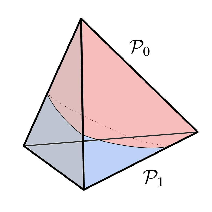
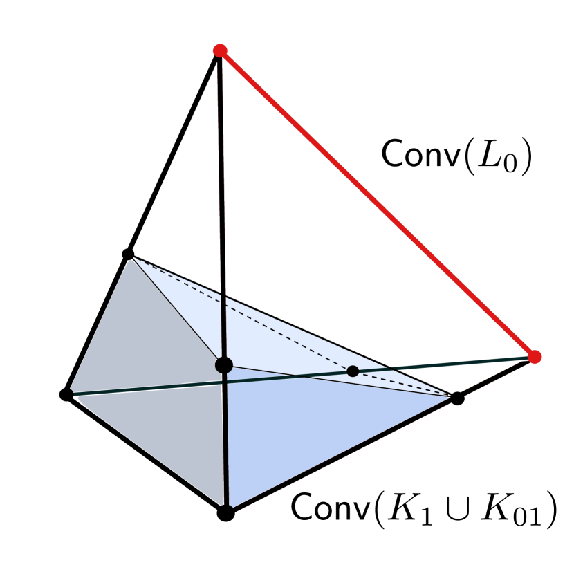
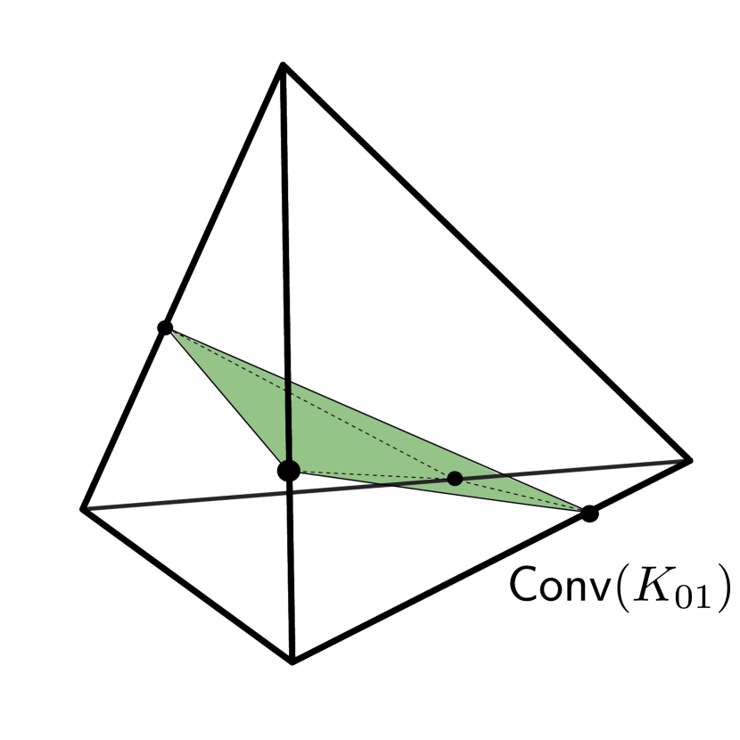
Figure 7: Geometry of $\Delta(\Omega)$ when $\mathsf{Conv}(K_{01})$ is not a hyperplane. Here, $\mathsf{Conv}(L_{0})$ is an edge of the simplex, shown in red.

Recall that $L_{0}\triangleq K_{0}\cap K_{1}^{c}$ denotes the set of states for which action $0$ is uniquely optimal for the receiver.

Lemma 11.2

$\Delta(\Omega)=\mathsf{Conv}(L_{0}\cup K_{01})\cup\mathsf{Conv}(K_{1}\cup K_{01})$.

Proof 11.3

Proof. Let $\mu\in\Delta(\Omega)$. Since $\Omega=L_{0}\cup K_{1}$, we have $\mu\in\mathsf{Conv}(L_{0}\cup K_{1})=\mathsf{Conv}(L_{0}\cup K_{1}\cup K_{01})$. Consider any convex decomposition of $\mu=\sum_{\phi\in L_{0}\cup K_{1}\cup K_{01}}\alpha_{\phi}\phi$. If the convex decomposition does not place positive weights either on the elements of $L_{0}$ or on those of $K_{1}\setminus K_{01}$, then we are done. Otherwise, let $\omega_{0}\in L_{0}$ and $\omega_{1}\in K_{1}\setminus K_{01}$ be such that $\alpha_{\phi}>0$ for $\phi\in\{\omega_{0},\omega_{1}\}$. Let $\mu^{\prime}\triangleq\frac{1}{\alpha_{\omega_{0}}+\alpha_{\omega_{1}}}(\alpha_{\omega_{0}}\omega_{0}+\alpha_{\omega_{1}}\omega_{1})$, and note that $\mu=(\alpha_{\omega_{0}}+\alpha_{\omega_{1}})\mu^{\prime}+\sum_{\phi\in L_{0}\setminus\{\omega_{0}\}}\alpha_{\phi}\phi+\sum_{\phi\in K_{01}\cup K_{1}\setminus\{\omega_{1}\}}\alpha_{\phi}\phi$. Since $\mu^{\prime}\in\mathsf{Conv}(\{\omega_{0},\omega_{1}\})$, one can write $\mu^{\prime}$ as either a convex combination of $\omega_{0}$ and $\chi(\omega_{0},\omega_{1})$ or a convex combination of $\omega_{1}$ and $\chi(\omega_{0},\omega_{1})$. In either scenario, using this decomposition for $\mu^{\prime}$, we obtain a convex decomposition of $\mu$ that places positive weight on at least one fewer element of $L_{0}\cup(K_{1}\setminus K_{01})$. Continuing with this process, we obtain a convex decomposition of $\mu$ that places no positive weight either on elements on $L_{0}$ or on elements of $K_{1}\setminus K_{01}$, yielding the lemma statement.

The second lemma uses this result to establish that $\mathsf{Conv}(\mathcal{P}_{1})$ is a convex polytope with extreme points in the set $K_{1}\cup K_{01}$.

Lemma 11.4

Under Assumption 5.1, $\mathsf{Conv}(\mathcal{P}_{1})=\mathsf{Conv}(K_{1}\cup K_{01})$.

Proof 11.5

Proof. We have $K_{1}\subseteq\mathcal{P}_{1}$, and furthermore, as $\cal{P}_{1}$ is closed, we have $K_{01}\subseteq\mathcal{P}_{1}$. Hence, we obtain that $\mathsf{Conv}(K_{1}\cup K_{01})\subseteq\mathsf{Conv}(\mathcal{P}_{1})$. Thus, to prove the lemma statement, we must show $\mathsf{Conv}(\mathcal{P}_{1})\subseteq\mathsf{Conv}(K_{1}\cup K_{01})$. Morever, since $\mathsf{Conv}(\mathcal{P}_{1})$ is the smallest convex set containing $\mathcal{P}_{1}$, it suffices to show $\mathcal{P}_{1}\subseteq\mathsf{Conv}(K_{1}\cup K_{01})$.

Let $\mu\in\mathcal{P}_{1}$. By Lemma 11.2, $\mu\in\mathsf{Conv}(L_{0}\cup K_{01})\cup\mathsf{Conv}(K_{1}\cup K_{01})$. Suppose for the sake of contradition, $\mu\notin\mathsf{Conv}(K_{1}\cup K_{01})$. Then, it follows that $\mu\in\mathsf{Conv}(L_{0}\cup K_{01})$ and $\mu\notin\mathsf{Conv}(K_{01})$. Consider any convex decomposition of $\mu$ as follows:

$$\mu=\sum_{\omega\in L_{0}}\alpha_{\omega}^{0}\omega+\sum_{\omega\in K_{01}\cap K_{1}}\alpha_{\omega}^{0}\omega+\sum_{\phi\in K_{01}\cap K_{1}^{c}}\alpha_{\phi}^{0}\phi.$$

Define $H_{0}^{0}=\{\omega\in L_{0}:\alpha_{\omega}^{0}>0\}$, $H_{0}^{1}=\{\omega\in K_{01}\cap K_{1}:\alpha_{\omega}^{0}>0\}$, and $H_{0}^{2}=\{\phi\in K_{01}\cap K_{1}^{c}:\alpha_{\phi}^{0}>0\}$. Since $\mu\notin\mathsf{Conv}(K_{01})$, it follows that $\sum_{\omega\in L_{0}}\alpha_{\omega}^{0}>0$. Thus, we obtain that $H_{0}^{0}$ is non-empty.

In the following, we inductively define sets $\{H_{n}^{i}:i=0,1,2\}$ for $n\geq 1$ as long as both $H_{n-1}^{0}$ and $H_{n-1}^{1}$ are non-empty, such that the following four properties hold: (1) $H_{n}^{0}\subseteq L_{0}$; (2) $H_{n}^{1}\subseteq K_{01}\cap K_{1}$; (3) for any $\chi(\omega_{0},\omega_{1})\in H_{n}^{2}\subseteq K_{01}$, either $\chi(\omega_{0},\omega_{1})\in K_{01}\cap K_{1}^{c}$ or $\omega_{0}\in H_{n}^{0}$; and (4) $\mu$ is a strict convex combination of elements in $H_{n}^{0}\cup H_{n}^{1}\cup H_{n}^{2}$. Towards that end, first note that the sets $\{H_{0}^{i}:i=0,1,2\}$ satisfy the aforementioned four properties.

Next, suppose for some $n\geq 1$ the sets $\{H_{n-1}^{i}:i=0,1,2\}$ satisfy the four properties, with both $H_{n-1}^{0}$ and $H_{n-1}^{1}$ being non-empty. Consider a strict convex decomposition of $\mu$ in terms of elements in $\cup_{i=0}^{2}H_{n-1}^{i}$ with coefficients $\alpha^{n-1}_{\phi}>0$ for $\phi\in\cup_{i=0}^{2}H_{n-1}^{i}$. Choose some $\omega_{0}\in H_{n-1}^{0}$ and $\omega_{1}\in H_{n-1}^{1}$, and let $\beta_{n-1}=\alpha_{\omega_{0}}^{n-1}/(\alpha_{\omega_{0}}^{n-1}+\alpha_{\omega_{1}}^{n-1})$. Observe that $\beta_{n-1}\omega_{0}+(1-\beta_{n-1})\omega_{1}$ either (1) equals $\chi(\omega_{0},\omega_{1})$; or (2) is a strict convex combination of $\omega_{0}$ and $\chi(\omega_{0},\omega_{1})$; or (3) is a strict convex combination of $\chi(\omega_{0},\omega_{1})$ and $\omega_{1}$. We split the analysis into the three respective cases:

1. If $\beta_{n-1}\omega_{0}+(1-\beta_{n-1})\omega_{1}$ equals $\chi(\omega_{0},\omega_{1})$, let $H_{n}^{i}=H_{n-1}^{i}\setminus\{\omega_{i}\}$ for $i\in\{0,1\}$ and $H_{n}^{2}=H_{n-1}^{2}\cup\{\chi(\omega_{0},\omega_{1})\}$. Since $\alpha_{\omega_{i}}^{n-1}>0$ for $i\in\{0,1\}$, we have $\beta_{n-1}\in(0,1)$ and hence $\chi(\omega_{0},\omega_{1})\in K_{01}\cap K_{1}^{c}$. Finally, letting $\alpha^{n}_{\phi}=\alpha^{n-1}_{\phi}$ for all $\phi\in\cup_{i=0}^{2}H_{n}^{i}\setminus\{\chi(\omega_{0},\omega_{1})\}$ and $\alpha^{n}_{\phi}=(\alpha_{\phi}^{n-1}+\alpha^{n-1}_{\omega_{0}}+\alpha^{n-1}_{\omega_{1}})>0$ for $\phi=\chi(\omega_{0},\omega_{1})$, we obtain a strict convex combination of $\mu$ in terms of elements of $\cup_{i=0}^{2}H_{n}^{i}$. Thus, the four properties continue to hold for $\{H_{n}^{i}:i=0,1,2\}$.

2. If $\beta_{n-1}\omega_{0}+(1-\beta_{n-1})\omega_{1}$ is a strict convex combination of $\omega_{0}$ and $\chi(\omega_{0},\omega_{1})$, let $H_{n}^{0}=H_{n-1}^{0}$, $H_{n}^{1}=H_{n-1}^{1}\setminus\{\omega_{1}\}$ and $H_{n}^{2}=H_{n-1}^{2}\cup\{\chi(\omega_{0},\omega_{1})\}$. Note that properties (1) and (2) hold trivially, and since $\omega_{0}\in H_{n}^{0}$, property (3) continues to hold. Using the strict convex combination of $\beta_{n-1}\omega_{0}+(1-\beta_{n-1})\omega_{1}$ in terms of $\omega_{0}$ and $\chi(\omega_{0},\omega_{1})$, we obtain a strict convex combination of $\mu$ in terms of elements of $\cup_{i=0}^{2}H_{n}^{i}$, and hence property (4) also holds.

3. If $\beta_{n-1}\omega_{0}+(1-\beta_{n-1})\omega_{1}$ is a strict convex combination of $\chi(\omega_{0},\omega_{1})$ and $\omega_{1}$, let $H_{n}^{0}=H_{n-1}^{0}\setminus\{\omega_{0}\}$, $H_{n}^{1}=H_{n-1}^{1}$ and $H_{n}^{2}=H_{n-1}^{2}\cup\{\chi(\omega_{0},\omega_{1})\}$. Again, properties (1) and (2) hold trivially. Since $\beta_{n-1}\omega_{0}+(1-\beta_{n-1})\omega_{1}$ with $\beta_{n-1}\in(0,1)$ is a strict convex combination of $\chi(\omega_{0},\omega_{1})$ and $\omega_{1}$, it follows that $\chi(\omega_{0},\omega_{1})\neq\omega_{1}$ and hence $\chi(\omega_{0},\omega_{1})\in K_{01}\cap K_{1}^{c}$. Thus property (3) holds. Finally, using the strict convex combination of $\beta_{n-1}\omega_{0}+(1-\beta_{n-1})\omega_{1}$ in terms of $\chi(\omega_{0},\omega_{1})$ and $\omega_{1}$, we obtain a strict convex combination of $\mu$ in terms of elements of $\cup_{i=0}^{2}H_{n}^{i}$, and hence property (4) also holds.

Note that in all three cases, we have $|H_{n}^{0}|+|H_{n}^{1}|<|H_{n-1}^{0}|+|H_{n-1}^{1}|$. Thus, this inductive process stops with sets $H_{n}^{i},i=0,1,2$ for some $n\geq 0$ with either $H_{n}^{0}$ or $H_{n}^{1}$ empty. If $H_{n}^{0}$ is empty, then $\mu\in\mathsf{Conv}(H_{n}^{1}\cup H_{n}^{2})\subseteq\mathsf{Conv}(K_{01})$, contradicting the assumption that $\mu\notin\mathsf{Conv}(K_{01}\cup K_{1})$. Thus, it must be that $H_{n}^{1}$ is empty. Furthermore, consider any $\phi=\chi(\omega_{0},\omega_{1})\in H_{n}^{2}$ for which $\omega_{0}\notin H_{n}^{0}$. By property (3), it must be that $\chi(\omega_{0},\omega_{1})\in K_{01}\cap K_{1}^{c}$. Choose any $\omega^{\prime}\in H_{n}^{0}$, and define $\beta=\alpha_{\omega^{\prime}}^{n}/(\alpha_{\omega^{\prime}}^{n}+\alpha_{\phi}^{n})$. Since $\chi(\omega_{0},\omega_{1})\in K_{01}\cap K_{1}^{c}$ and $\omega^{\prime}\in H_{n}^{0}$, it is straightforward to verify that $\beta\omega^{\prime}+(1-\beta)\chi(\omega_{0},\omega_{1})$ can be written as a strict convex combination of $\omega_{0}$, $\omega^{\prime}$, $\chi(\omega_{0},\omega_{1})$ and $\chi(\omega^{\prime},\omega_{1})$. Using such a strict convex combination and adding $\omega_{0}\in L_{0}$ to the set $H_{n}^{0}$ (and if needed, adding $\chi(\omega^{\prime},\omega_{1})$ to $H_{n}^{2}$), we can without loss of generality assume that for any $\phi=\chi(\omega_{0},\omega_{1})\in H_{n}^{2}$ we have $\omega_{0}\in H_{n}^{0}$. We thus obtain the following strict convex decomposition:

$$\mu=\sum_{\omega\in H_{n}^{0}}\gamma_{\omega}\omega+\sum_{\phi\in H_{n}^{2}}\gamma_{\phi}\phi,$$

where $\sum_{\omega\in H_{n}^{0}}\gamma_{\omega}>0$, and for which if $\chi(\omega_{0},\omega_{1})\in H_{n}^{2}$ then $\omega_{0}\in H_{n}^{0}$.

This can be further rewritten as the following convex combination

$$\mu=\sum_{\omega\in H_{n}^{0}}\hat{\gamma}_{\omega}\omega+\sum_{\chi(\omega_{0},\omega_{1})\in H_{n}^{2}}(\tilde{\gamma}_{\omega_{0}}\omega_{0}+\tilde{\gamma}_{\chi(\omega_{0},\omega_{1})}\chi(\omega_{0},\omega_{1})),$$

where if $\tilde{\gamma}_{\chi(\omega_{0},\omega_{1})}>0$, then $\tilde{\gamma}_{\omega_{0}}>0$. Note that for any such $(\omega_{0},\omega_{1})$, by definition of $\chi(\omega_{0},\omega_{1})$, the belief $\xi(\omega_{0},\omega_{1})\triangleq\frac{1}{(\tilde{\gamma}_{\omega_{0}}+\tilde{\gamma}_{\chi(\omega_{0},\omega_{1})})}\left(\tilde{\gamma}_{\omega_{0}}\omega_{0}+\tilde{\gamma}_{\chi(\omega_{0},\omega_{1})}\chi(\omega_{0},\omega_{1})\right)$ lies in the set $\mathcal{P}_{1}^{c}$. Thus, $\mu$ is a convex combination of elements in $H_{n}^{0}\subseteq L_{0}$ and the elements $\{\xi(\omega_{0},\omega_{1})\}$, all of which belong to $\mathcal{P}_{1}^{c}$. From Assumption 5.1, we then obtain that $\mu$ itself is an element of $\mathcal{P}_{1}^{c}$, contradicting the fact that $\mu\in\mathcal{P}_{1}$. This proves that our initial assumption that $\mu\notin\mathsf{Conv}(K_{1}\cup K_{01})$ must be false, and hence $\mu\in\mathsf{Conv}(K_{1}\cup K_{01})$.

Thus, $\mu\in\mathcal{P}_{1}$ implies $\mu\in\mathsf{Conv}(K_{1}\cup K_{01})$, and hence $\mathcal{P}_{1}\subseteq\mathsf{Conv}(K_{1}\cup K_{01})$. Thus, we conclude that $\mathsf{Conv}(\mathcal{P}_{1})=\mathsf{Conv}(K_{1}\cup K_{01})$.

With these two helper lemmas in place, we are now ready to prove Theorem 5.2.

Proof 11.6

Proof of Theorem 5.2. Since the objectives of the programs (7) and (10) are identical, to prove the result it suffices to show that optimal solution of each program is a feasible for the other.

First, consider any optimal solution to (10). Since $\mathsf{Conv}(L_{0}\cup\{\mathbf{0}\})\subseteq\mathsf{Conv}(\mathcal{P}_{0}\cup\{\mathbf{0}\})$ and $\mathsf{Conv}(K_{1}\cup K_{01}\cup\{\mathbf{0}\})\subseteq\mathsf{Conv}(\mathcal{P}_{1}\cup\{\mathbf{0}\})$, it is a feasible solution to (7).

Next, consider any optimal solution $t=(t_{0},t_{1})$ to (7) with $t_{1}\in\mathsf{Conv}(\mathcal{P}_{1}\cup\{\mathbf{0}\})$ and $t_{0}\in\mathsf{Conv}(\mathcal{P}_{0}\cup\{\mathbf{0}\})$. By Lemma 11.4, it follows that $t_{1}\in\mathsf{Conv}(K_{1}\cup K_{01}\cup\{\mathbf{0}\})$. If $t_{0}=\mathbf{0}$, then $t_{0}\in\mathsf{Conv}(L_{0}\cup\{\mathbf{0}\})$ and we are done. Instead, suppose $t_{0}\neq\mathbf{0}$. Let $t_{0}=b_{0}m_{0}$ where $b_{0}\in(0,1]$ and $m_{0}\in\mathsf{Conv}(\mathcal{P}_{0})$. By Lemma 11.2, we obtain $m_{0}\in\mathsf{Conv}(L_{0}\cup K_{01})\cup\mathsf{Conv}(K_{1}\cup K_{01})$. If $m_{0}\in\mathsf{Conv}(K_{1}\cup K_{01})$, then the solution $\hat{t}=(\hat{t}_{0},\hat{t}_{1})$ with $\hat{t}_{0}=0$ and $\hat{t}_{1}=t_{1}+t_{0}$ is feasible for (7) and achieves larger utility for the sender than $(t_{0},t_{1})$, contradicting the latter’s optimality. Hence, $m_{0}\in\mathsf{Conv}(L_{0}\cup K_{01})$. If $m_{0}\notin\mathsf{Conv}(L_{0})$, then $m_{0}=(1-\alpha)\nu_{0}+\alpha\nu_{1}$ with $\nu_{0}\in\mathsf{Conv}(L_{0})$ and $\nu_{1}\in\mathsf{Conv}(K_{01})$ and $\alpha>0$. However, we then have that $\tilde{t}=(\tilde{t}_{0},\tilde{t}_{1})$ with $\tilde{t}_{0}=b_{0}(1-\alpha)\nu_{0}$ and $\tilde{t}_{1}=t_{1}+b_{0}\alpha\nu_{1}$ is feasible for (7) and has larger utility for the sender than $(t_{0},t_{1})$, once again contradicting the latter’s optimality. Thus, we must have $m_{0}\in\mathsf{Conv}(L_{0})$ and hence $t_{0}\in\mathsf{Conv}(L_{0}\cup\{\mathbf{0}\})$. Taken together, we obtain that $(t_{0},t_{1})$ is feasible for (10).

Finally, we conclude this section with the proof of Proposition 5.3.

Proof 11.7

Proof of Proposition 5.3. First, note that if $v(\omega,1)-v(\omega,0)=v>0$ for all $\omega\in\Omega$, then for any feasible $t=(t_{0},t_{1})$ for (10), we have $\sum_{\omega\in\Omega}v(\omega,1)t_{1}(\omega)+v(\omega,0)t_{0}(\omega)=\sum_{\omega\in\Omega}v(\omega,0)\mu^{*}(\omega)+v\sum_{\omega\in\Omega}t_{1}(\omega)$. Thus, it suffices to show that for any $t=(t_{0},t_{1})$ that does not have the threshold structure, one can find another feasible $\tilde{t}=(\tilde{t}_{1},\tilde{t}_{0})$ that satisfies $\sum_{\omega\in\Omega}t_{1}(\omega)<\sum_{\omega\in\Omega}\tilde{t}_{1}(\omega)$.

Toward that end, let $t=(t_{0},t_{1})$ be a feasible solution to (10) such that there exists $\omega^{\dagger},\omega^{\prime}\in\Omega$ satisfying $\omega^{\dagger}\prec\omega^{\prime}$ with $t_{1}(\omega^{\dagger})<\mu^{*}(\omega^{\dagger})$ and $t_{1}(\omega^{\prime})>0$. Since $t_{1}+t_{0}=\mu^{*}$, we obtain $t_{0}(\omega^{\dagger})>0$. As $t_{0}\in\mathsf{Conv}(L_{0}\cup\{\mathbf{0}\})$, this implies that $\omega^{\dagger}\in L_{0}$. By Assumption 5.2, this implies that $\omega^{\prime}\in L_{0}$ as well.

Now, $t_{1}\in\mathsf{Conv}(K_{1}\cup K_{01}\cup\{\mathbf{0}\})$ implies that

$$t_{1}=\sum_{j\in K_{1}}\alpha_{j}e_{j}+\sum_{\phi\in K_{01}\setminus K_{1}}\alpha_{\phi}\phi,$$

with $\alpha_{j},\alpha_{\phi}\geq 0$ and $\sum_{j\in K_{1}}\alpha_{j}+\sum_{\phi\in K_{01}\setminus K_{1}}\alpha_{\phi}\leq 1$. Since $t_{1}(\omega^{\prime})>0$, we deduce that there exists an $\hat{\omega}\in K_{1}$ such that $\alpha_{\phi}>0$ for $\phi=\chi(\omega^{\prime},\hat{\omega})$. For fixed small enough $\epsilon>0$, define $\tilde{t}=(\tilde{t}_{0},\tilde{t}_{1})$ as

$$\tilde{t}_{1} =t_{1}+\epsilon\chi(\omega^{\dagger},\hat{\omega})-\epsilon^{\prime}\chi(\omega^{\prime},\hat{\omega})$$

$$\tilde{t}_{0} =t_{0}-\epsilon\chi(\omega^{\dagger},\hat{\omega})+\epsilon^{\prime}\chi(\omega^{\prime},\hat{\omega}),$$

where $\epsilon^{\prime}>0$ satisfies $\epsilon^{\prime}(1-\gamma(\omega^{\prime},\hat{\omega}))=\epsilon(1-\gamma(\omega^{\dagger},\hat{\omega}))$. Clearly, we have $\tilde{t}_{1}+\tilde{t}_{0}=t_{1}+t_{0}=\mu^{*}$. Furthermore, for small enough $\epsilon>0$, we have $\tilde{t}_{1}\in\mathsf{Conv}(K_{1}\cup K_{01}\cup\{\mathbf{0}\})$. Finally, using the definition of $\chi(\omega^{\dagger},\hat{\omega})$ and $\chi(\omega^{\prime},\hat{\omega})$ and the choice of $\epsilon^{\prime}$, we have

$$\tilde{t}_{0} =t_{0}-\epsilon\gamma(\omega^{\dagger},\hat{\omega})e_{\omega^{\dagger}}+\epsilon^{\prime}\gamma(\omega^{\prime},\hat{\omega})e_{\omega^{\prime}}.$$

Since $t_{0}\in\mathsf{Conv}(L_{0}\cup\{\mathbf{0}\})$ with $t_{0}(\omega^{\dagger})>0$, and $\omega^{\prime}\in L_{0}$, we obtain that $\tilde{t}_{0}\in\mathsf{Conv}(L_{0}\cup\{\mathbf{0}\})$ for small enough $\epsilon>0$. Thus, putting it all together, for small enough $\epsilon>0$, $\tilde{t}$ is feasible for (10).

Finally, we have

$$\sum_{\omega\in\Omega}\tilde{t}_{1}(\omega) =\sum_{\omega\in\Omega}t_{1}(\omega)+\epsilon\gamma(\omega^{\dagger},\hat{\omega})-\epsilon^{\prime}\gamma(\omega^{\prime},\hat{\omega})$$

$$=\sum_{\omega\in\Omega}t_{1}(\omega)+\epsilon(1-\gamma(\omega^{\dagger},\hat{\omega}))\left(\frac{\gamma(\omega^{\dagger},\hat{\omega})}{1-\gamma(\omega^{\dagger},\hat{\omega})}-\frac{\gamma(\omega^{\prime},\hat{\omega})}{1-\gamma(\omega^{\prime},\hat{\omega})}\right)$$

$$>\sum_{\omega\in\Omega}t_{1}(\omega),$$

where we have used the fact that since $\omega^{\dagger}\prec\omega^{\prime}$, we have $\gamma(\omega^{\dagger},\hat{\omega})>\gamma(\omega^{\prime},\hat{\omega})$.

12 Proofs from Section 7

In this section, we provide the proofs of the results from Section 7. To begin, let $\Omega=\{0,1,\ldots,C-1\}$ denote the set of queue-lengths for which an arriving customer could possibly join the queue. (We assume that immediately upon arrival a customer is informed whether the queue-length equals $C$ or not.) Let $X$ denote the waiting time until service completion faced by an arriving customer if she decides to join the queue. Under the belief $e_{n}$, an arriving customer knows that there are exactly $n$ customers already in queue, and thus $X$ has the distribution of the sum of $n+1$ independent unit exponential random variables.

Recall the definition (11) of the differential utility function: $\hat{\rho}(\mu)=\tau-\left(\operatorname{\mathbf{E}}_{\mu}[X]+\beta\sqrt{\operatorname{\mathrm{Var}}_{\mu}[X]}\right)$ for some $\tau>0$ and $\beta\geq 0$. It is straightforward to verify that $\hat{\rho}(e_{n})=\tau-\left(n+1+\beta\sqrt{n+1}\right)$, and hence $\hat{\rho}(e_{n})$ is strictly decreasing in $n$. As $K_{1}=\{n\in\Omega:\hat{\rho}(e_{n})\geq 0\}$, and $L_{0}=\{n\in\Omega:\hat{\rho}(e_{n})<0\}$, we obtain that $K_{1}=\{0,1,\ldots,M\}$ and $L_{0}=\{n\in\Omega:n>M\}$ for some $M<C$.

For $n,m\in\Omega$ and $\gamma\in[0,1]$, the belief $\mu=\gamma e_{n}+(1-\gamma)e_{m}$ assigns probability $\gamma$ to the state with $n$ customers already in queue, and probability $1-\gamma$ to the state with $m$ customers already in queue; consequently, under the belief $\mu$, the distribution of $X$ is a convex mixture (with weight $\gamma$) of its distribution under beliefs $e_{n}$ and $e_{m}$. Thus, we obtain $\operatorname{\mathbf{E}}_{\mu}[X]=1+m+(n-m)\gamma$ and $\operatorname{\mathrm{Var}}_{\mu}[X]=1+m+(n-m)\gamma+(n-m)^{2}\gamma(1-\gamma)$. Finally, for $n\in L_{0}$ and $m\in K_{1}$, $\gamma(n,m)=\sup\{\gamma\in[0,1]:\hat{\rho}(\gamma e_{n}+(1-\gamma)e_{m})\geq 0\}$ is the largest value of $\gamma\in[0,1]$ for which $\gamma e_{n}+(1-\gamma)e_{m}\in\mathcal{P}_{1}$, and $\chi(n,m)=\gamma(n,m)e_{n}+(1-\gamma(n,m))e_{m}$ is the corresponding belief. Note that under the belief $\chi(n,m)$, the customer is indifferent between joining and leaving the queue. Using the expression for $\hat{\rho}$ and after some straightforward algebra, we obtain for $n\in L_{0}$ and $m\in K_{1}$,

$$\gamma(n,m)=\frac{2(\tau-1-m)+\beta^{2}(n-m+1)-\beta\sqrt{h(n,m)}}{2(n-m)(1+\beta^{2})},$$ (15)

where $h(n,m)\triangleq\beta^{2}(n-m+1)^{2}+4(\tau-1-m)(n-m+1)+4(1+\beta^{2})(1+m)-4(\tau-1-m)^{2}$.

The following result implies that differential utility function $\hat{\rho}(\cdot)$ defined in (11) is convex and monotone (Assumptions 5.1 and 5.2).

Lemma 12.1

For $\tau>0,\beta\geq 0$, let $\hat{\rho}(\mu)=\tau-\left(\operatorname{\mathbf{E}}_{\mu}[X]+\beta\sqrt{\operatorname{\mathrm{Var}}_{\mu}[X]}\right)$. Then,

1. The differential utility function $\hat{\rho}(\mu)$ is convex in $\mu$, and hence satisfies Assumption 5.1.

2. Under the usual total order on $\Omega$, $\hat{\rho}(\mu)$ satisfies the monotonicity condition in Assumption 5.2.

Proof 12.2

Proof. From the fact that expectation is linear in the belief, it is straightforward to show that $\operatorname{\mathrm{Var}}_{\mu}[X]=\operatorname{\mathbf{E}}_{\mu}\left(X^{2}\right)-\left(\operatorname{\mathbf{E}}_{\mu}(X)\right)^{2}$ is concave in the belief $\mu$. Since $\sqrt{x}$ is concave and strictly increasing in $x$, using Jensen’s inequality, we obtain that $\sqrt{\operatorname{\mathrm{Var}}_{\mu}[X]}$ is also concave in $\mu$. From these facts, we conclude that $\hat{\rho}(\mu)=\tau-\left(\operatorname{\mathbf{E}}_{\mu}[X]+\beta\sqrt{\operatorname{\mathrm{Var}}_{\mu}[X]}\right)$ is convex in $\mu$. Thus, we obtain that the set $\mathcal{P}_{a}^{c}=\{\mu:\hat{\rho}(\mu)<0\}$ is convex, and hence $\hat{\rho}(\cdot)$ satisfies Assumption 5.1.

Since $K_{1}=\{0,1,\ldots,M\}$ and $L_{0}=\{n\in\Omega:n>M\}$, if $m\in K_{1}$ then $m<n$ for all $n\in L_{0}$. Next, let $m\in K_{1}$ and $n,\ell\in L_{0}$ with $n<\ell$. For $\gamma\in(0,1]$, let $\mu=\gamma e_{n}+(1-\gamma)e_{m}$ and $\mu^{\prime}=\gamma e_{\ell}+(1-\gamma)e_{m}$. Since $\operatorname{\mathbf{E}}_{\mu}[X]<\operatorname{\mathbf{E}}_{\mu^{\prime}}[X]$ and $\operatorname{\mathrm{Var}}_{\mu}[X]<\operatorname{\mathrm{Var}}_{\mu^{\prime}}[X]$, we obtain that $\hat{\rho}(\mu)>\hat{\rho}(\mu^{\prime})$ for all $\gamma\in(0,1]$. Thus, we obtain that $\gamma(n,m)>\gamma(\ell,m)$. To summarize, the usual order on $\Omega$ satisfies the property that if $n<\ell$, then either $n\in K_{1}$ or for all $m\in K_{1}$, we have $\gamma(n,m)>\gamma(\ell,m)$. Thus, we obtain that $\hat{\rho}(\cdot)$ satisfies the monotonicity condition (Assumption 5.2).

12.1 Proof of Lemma 7.1

Our proof follows a similar approach as in Lingenbrink and Iyer (2019): we show that any feasible solution where the customers’ actions do not have a threshold structure can be perturbed to obtain another feasible solution corresponding to a signaling scheme with higher throughput.

Proof 12.3

Proof of Lemma 7.1. First, note that if $K_{1}=\Omega$. i.e., $M=C-1$, then joining the queue is always optimal. In this case, the full-information mechanism (a mechanism inducing a threshold structure on the actions) has the highest throughput. Hence, hereafter we focus on the case where $K_{1}$ is a strict subset of $\Omega$, i.e, $M<C-1$.

Consider a feasible solution $t=(t_{1},t_{0})$ to the linear program (12). Since $t_{0}\in\mathsf{Conv}(L_{0}\cup\{\mathbf{0}\})$ and $L_{0}=\{M+1,\ldots,C-1\}$, we have $t_{0}(k)=0$ for all $k\leq M$. Then the constraint (12c) implies that $t_{1}(k+1)=\lambda t_{1}(k)$ for all $k<M$, and hence $t_{1}(k)=\lambda^{k}t_{1}(0)$ for all $k\leq M$.

Let $N$ be the largest value of $n$ such that $t_{1}(k)=\lambda^{k}t_{1}(0)$ for all $k\leq n$. (Note the preceding argument implies $N\geq M$.) If either $N\geq C-2$ or $t_{1}(N+2)=0$, then we obtain that $t$ induces a threshold structure in the customers’ actions. Hence, for the rest of the proof assume that $N<C-2$ and $t_{1}(N+2)>0$. Using (12c), we then obtain $0<t_{1}(N+1)<\lambda t_{1}(N)$, $t_{0}(N+1)>0$ and $t_{0}(n)=0$ for $n\leq N$. We now show that $t=(t_{1},t_{0})$ cannot be an optimal solution to (12). We do this by constructing another feasible solution $\tilde{t}=(\tilde{t}_{1},\tilde{t}_{0})$ that has a larger objective value than $t$.

For some small $\epsilon>0$ and $\beta>0$ to be chosen later, consider $\tilde{t}=(\tilde{t}_{1},\tilde{t}_{0})$ with

$$\tilde{t}_{1} =\frac{1}{Z}\left(t_{1}-\beta\sum_{m=N+2}^{C-1}t_{1}(m)e_{m}+(\beta+\epsilon)\sum_{m=N+2}^{C-1}t_{1}(m)e_{N+1}\right)$$

and $\tilde{t}_{0}(0)=0$, $\tilde{t}_{0}(n)=\lambda\tilde{t}_{1}(n-1)-\tilde{t}_{1}(n)$ for all $n>0$, where $Z$ is chosen to satisfy (12d); it is straightforward to verify that

$$Z=1+\lambda\epsilon\sum_{m=N+2}^{C-1}t_{1}(m).$$

In particular, for $\epsilon>0$, we obtain that $Z>1$.

We begin by showing that $\tilde{t}$ is feasible for (12) for all small enough $\epsilon,\beta>0$. Note that $\tilde{t}$ satisfies (12c) and (12d) by definition. Thus, we verify the conditions (12a) and (12b).

First, note that for $\ell\leq N$, we have $\tilde{t}_{1}(\ell)=\frac{1}{Z}t_{1}(\ell)$. On the other hand, we have $\tilde{t}_{1}(N+1)=\frac{1}{Z}(t_{1}(N+1)+(\beta+\epsilon)\sum_{m=N+2}^{C-1}t_{1}(m))$ and $\tilde{t}_{1}(\ell)=\frac{(1-\beta)}{Z}t_{1}(\ell)$ for $\ell>N+1$. Using this and the definition of $\tilde{t}_{0}$, it is straightforward to verify that for small enough $\epsilon,\beta>0$, we have $\tilde{t}_{0}\geq 0$ and $\tilde{t}_{0}(0)=0$ for all $\ell\leq N$. Further using the fact that $\sum_{\ell}\tilde{t}_{0}(\ell)\leq 1$, we obtain $\tilde{t}_{0}\in\mathsf{Conv}(L_{0}\cup\{\mathbf{0}\})$ for all small enough $\epsilon,\beta>0$, and hence $\tilde{t}$ satisfies (12a).

Next, since $t_{1}\in\mathsf{Conv}(K_{1}\cup K_{01}\cup\{\mathbf{0}\})$, we can write the decomposition

$$t_{1} =\sum_{j=0}^{M}\alpha(j)e_{j}+\sum_{j=0}^{M}\sum_{i=M+1}^{C-1}\delta(i,j)\chi(i,j),$$

where $\alpha(j)\geq 0$ for $j\leq M$, $\delta(i,j)\geq 0$ for $j\leq M<i$, and $\sum_{j=0}^{M}\alpha(j)+\sum_{j=0}^{M}\sum_{i=M+1}^{C-1}\delta(i,j)\leq 1$. Thus, we have

$$Z\tilde{t}_{1} =t_{1}-\beta\sum_{m=N+2}^{C-1}t_{1}(m)(e_{m}-e_{N+1})+\epsilon\sum_{m=N+2}^{C-1}t_{1}(m)e_{N+1}$$

$$=t_{1}-\beta\sum_{m=N+2}^{C-1}\sum_{j=0}^{M}\delta(m,j)\gamma(m,j)(e_{m}-e_{N+1})$$

$$\quad+\epsilon\sum_{m=N+2}^{C-1}\sum_{j=0}^{M}\delta(m,j)\gamma(m,j)e_{N+1}.$$

Now, it can be readily verified that for $0\leq j\leq M$ and $m>N+1$,

$$\gamma(m,j)(e_{m}-e_{N+1})=\chi(m,j)-\left(\frac{\gamma(m,j)}{\gamma(N+1,j)}\chi(N+1,j)+\left(1-\frac{\gamma(m,j)}{\gamma(N+1,j)}\right)e_{j}\right).$$

Thus, after some algebra, we obtain

$$Z\tilde{t}_{1} =t_{1}-\beta\sum_{m=N+2}^{C-1}\sum_{j=0}^{M}\delta(m,j)\chi(m,j)$$

$$\quad+\beta\sum_{m=N+2}^{C-1}\sum_{j=0}^{M}\delta(m,j)\left(\frac{\gamma(m,j)}{\gamma(N+1,j)}\chi(N+1,j)+\left(1-\frac{\gamma(m,j)}{\gamma(N+1,j)}\right)e_{j}\right)$$

$$\quad+\epsilon\sum_{m=N+2}^{C-1}\sum_{j=0}^{M}\delta(m,j)\gamma(m,j)e_{N+1}.$$

Now, since $t_{1}\in\mathsf{Conv}(K_{1}\cup K_{01}\cup\{\mathbf{0}\})$, we have the first term $t_{1}-\beta\sum_{m=N+2}^{C-1}\sum_{j=0}^{M}\delta(m,j)\chi(m,j)\in\mathsf{Conv}(K_{1}\cup K_{01}\cup\{\mathbf{0}\})$ for small enough $\beta>0$. Moreover, since $\hat{\rho}(\cdot)$ satisfies Assumption 5.2 (Lemma 12.1), we have $\gamma(N+1,j)>\gamma(m,j)$ for all $j\leq M$ and $m>N+1$. Hence, for all small enough $\beta>0$, we obtain that second term lies in the $\mathsf{Conv}(K_{1}\cup K_{01}\cup\{\mathbf{0}\})$, but not in $\mathsf{Conv}(K_{01}\cup\{\mathbf{0}\})$. This in turn implies that the second and the third term together lie in $\mathsf{Conv}(K_{1}\cup K_{01}\cup\{\mathbf{0}\})$ for small enough $\beta,\epsilon>0$. Taken together, this implies that $Z\tilde{t}_{1}$ (and hence $\tilde{t}_{1}$) lies in the cone generated by $\mathsf{Conv}(K_{1}\cup K_{01}\cup\{\mathbf{0}\})$. Since $\sum_{\omega}\tilde{t}_{1}(\omega)\leq 1$, we conclude that $\tilde{t}_{1}\in\mathsf{Conv}(K_{1}\cup K_{01}\cup\{\mathbf{0}\})$, and hence $\tilde{t}$ satisfies (12b).

Having shown the feasibility of $\tilde{t}$, we now verify that the objective value under $\tilde{t}$ is greater than that under $t$. Using (12d) and (12c), we obtain

$$\sum_{\ell=0}^{C-1}\tilde{t}_{1}(\ell) =\frac{1}{\lambda}\left(1-\tilde{t}_{1}(0)\right)>\frac{1}{\lambda}\left(1-t_{1}(0)\right)=\sum_{\ell=0}^{C-1}t_{1}(\ell).$$

Here, the inequality follows from the fact that $\tilde{t}_{1}(0)=\frac{1}{Z}t_{1}(0)<t_{1}(0)$ since $Z>1$. Thus, the objective of (12) for $\tilde{t}$ is strictly greater than that for $t$. Thus, it follows that $t$ cannot be optimal for (12).

To conclude the proof, we obtain from the preceding argument that for any optimal $t=(t_{1},t_{0})$, if $N$ denotes the largest value of $n$ such that $t_{1}(k)=\lambda^{k}t_{1}(0)$ for all $k\leq n$, then either $N\geq C-2$ or $t_{1}(N+2)=0$. In either case, we obtain that $t$ induces a threshold structure in the customers’ actions.

12.2 Proof of Proposition 7.2

Proof 12.4

Proof. The optimal signaling scheme can be found from the optimal solution to the linear program (12), using an argument similar to the discussion surrounding (8). Moreover, from similar argument as in Proposition 3.4, it follows that there exists an optimal signaling scheme that uses at most $|\Omega|=C$ signals per action. As $\hat{\rho}$ satisfies Assumption 5.1 (Lemma 12.1), all the signals that induce the customer to leave $(a=0)$ can be coalesced into single signal, which we call $\mathsf{Leave}$. Taken together, we obtain that there exists a signaling scheme with the signal set $\{\mathsf{Join}_{1},\mathsf{Join}_{2},\dots,\mathsf{Join}_{J},\mathsf{Leave}\}$ for some $J\leq|C|$, where each $\mathsf{Join}_{i}$ signal induces the customer to join the queue, and the $\mathsf{Leave}$ signal induces the customer to leave.

We will now show that there exists such an optimal signaling scheme that satisfies the three properties listed in the proposition statement. For ease of exposition, we will split the proof into three parts, one part for each property.

Part 1. From the constraints (12a) and (12b), we observe that the optimal signaling scheme can be implemented with the canonical set of join signals consisting of pure signals in $K_{1}$ and binary mixed signals in $K_{01}$. The customer’s utility upon receiving a binary mixed signal in $K_{01}$ or a signal in $K_{1}\cap K_{0}$ is zero by definition. Thus, to prove that a customer’s utility upon receiving each signal $\mathsf{Join}_{j}$ is zero, we need to prove that there exists a signaling scheme that never sends the pure signals in $K_{1}\cap K_{0}^{c}$. To show this, we use a perturbation argument, and show that any canonical signaling scheme that sends a pure signal in $K_{1}\cap K_{0}^{c}$ with positive probability must be sub-optimal.

Let $t=(t_{0},t_{1})$ be a feasible solution to (12) with $t_{0}\neq\mathbf{0}$. If $t$ does not have a threshold structure, then Lemma 7.1 implies that $t$ cannot be optimal for (12). Thus, henceforth we assume that $t$ has a threshold structure, i.e., there exists an $m\in L_{0}\cup\{C\}$ such that $t_{1}(\omega)>0$ for $\omega<m$, $t_{1}(\omega)=0$ for $\omega\geq m+1$, and $t_{0}(\omega)=0$ for $\omega\notin\{m,m+1\}$. Furthermore, since $\sum_{\omega\in\Omega}t_{0}(\omega)>0$, we obtain that $m<C$, and thus one can let $m\in L_{0}$ with $t_{0}(m)>0$.

Now, suppose $t_{1}\in\mathsf{Conv}(K_{1}\cup K_{01}\cup\{\mathbf{0}\})$ but $t_{1}\notin\mathsf{Conv}((K_{1}\cap K_{0})\cup K_{01}\cup\{\mathbf{0}\})$. The former condition implies that we can write $t_{1}$ as

$$t_{1}=\sum_{\omega_{1}\in K_{1}}\beta_{\omega_{1}}e_{\omega_{1}}+\sum_{\phi\in K_{01}\setminus K_{1}}\beta_{\phi}\phi.$$

where $\sum_{\omega_{1}\in K_{1}}\beta_{\omega_{1}}+\sum_{\phi\in K_{01}\setminus K_{1}}\beta_{\phi}\leq 1$. Furthermore, since $t_{1}\notin\mathsf{Conv}((K_{1}\cap K_{0})\cup K_{01}\cup\{\mathbf{0}\})$, it follows that there exists an $\omega_{1}^{*}\in K_{1}\cap K_{0}^{c}$ such that $\beta_{\omega_{1}^{*}}>0$. Using these facts, we will now construct a feasible $\hat{t}$ with strictly higher objective, thus implying that $t$ cannot be optimal.

For small enough $\epsilon>0$, let $\hat{t}=(\hat{t}_{0},\hat{t}_{1})$ be defined as

$$\hat{t}_{1} =\frac{1}{Z}\left(t_{1}+\epsilon e_{m}\right)$$

$$\hat{t}_{0} =\frac{1}{Z}\left(t_{0}-\epsilon e_{m}+\lambda\epsilon e_{m+1}\mathbf{I}\{m\neq C-1\}\right),$$

where $Z$ is chosen so that $\hat{t}$ satisfies (12d): $Z=1+\lambda\epsilon>1$. It is straightforward to verify that $\hat{t}$ satisfies (12c). Furthermore, since $t_{0}(m)>0$, we have for small enough $\epsilon>0$, $t_{0}-\epsilon e_{m}\in\mathsf{Conv}(L_{0}\cup\{\mathbf{0}\})$. Moreover, if $m\neq C-1$, then $e_{m+1}\in\mathsf{Conv}(L_{0}\cup\{\mathbf{0}\})$. This implies that $\hat{t}_{0}$ itself lies in $\mathsf{Conv}(L_{0}\cup\{\mathbf{0}\})$, and thus satisfies (12a).

Thus, to show the feasibility of $\hat{t}$, it remains to show that (12b) holds. We have

$$\hat{t}_{1} =\frac{1}{Z}\left(t_{1}+\epsilon e_{m}\right)$$

$$=\frac{1}{Z}\left(\sum_{\omega_{1}\in K_{1},\omega_{1}\neq\omega_{1}^{*}}\beta_{\omega_{1}}e_{\omega_{1}}+\sum_{\phi\in K_{01}\setminus K_{1}}\beta_{\phi}\phi\right)+\frac{1}{Z}\left(\beta_{\omega_{1}^{*}}e_{\omega_{1}^{*}}+\epsilon e_{m}\right).$$

Now, since $Z>1$, the first term lies in the set $\mathsf{Conv}(K_{1}\cup K_{01}\cup\{\mathbf{0}\})$. Furthermore, since $\omega_{1}^{*}\in K_{1}\in K_{0}^{c}$ and $m\in L_{0}$, for small enough $\epsilon>0$, the second term can be written as a convex combination of $\omega_{1}^{*}$, $\chi(m,\omega_{1}^{*})\in K_{01}$ and $\mathbf{0}$. Thus, we obtain that the second term lies in the set $\mathsf{Conv}(K_{1}\cup K_{01}\cup\{\mathbf{0}\})$ as well. Finally, since $\sum_{\omega\in\Omega}\hat{t}_{1}(\omega)=\frac{1}{Z}\left(\sum_{\omega\in\Omega}t_{1}(\omega)+\epsilon\right)=\frac{1}{Z}\left(1-\lambda t_{1}(C-1)-\sum_{\omega\in\Omega}t_{0}(\omega)+\epsilon\right)<1$ for small enough $\epsilon>0$, we obtain that $\hat{t}_{1}\in\mathsf{Conv}(K_{1}\cup K_{01}\cup\{\mathbf{0}\})$. Thus, $\hat{t}$ is feasible for (12).

Finally, note that,

$$\sum_{\omega\in\Omega}\hat{t}_{1}(\omega)-\sum_{\omega\in\Omega}t_{1}(\omega) =\frac{\epsilon}{Z}\left(1-\lambda\sum_{\omega\in\Omega}t_{1}(\omega)\right)>0,$$

where the final inequality follows from the fact that the throughput $\lambda\sum_{\omega\in\Omega}t_{1}(\omega)$ must be strictly less than the mean service rate, assumed to equal one. Thus, we obtain that $\hat{t}$ achieves a strictly higher objective than $t$, and hence $t$ cannot be optimal for (12). Summarizing, we obtain that any optimal $t=(t_{0},t_{1})$ with $t_{0}\neq\mathbf{0}$ must satisfy $t_{1}\in\mathsf{Conv}((K_{1}\cap K_{0})\cup K_{01}\cup\{\mathbf{0}\})$, and thus under the optimal signaling mechanism, for any signal that induces the customer to join, the induced beliefs are in the set $(K_{1}\cap K_{0})\cup K_{01}$, implying that her utility for joining must be zero.

Part 2. From the proof of part (1), it follows that for each $j\leq J$, the signal $\mathsf{Join}_{j}$ either induces a posterior belief $\omega^{j}\in K_{1}\cap K_{0}$ or a belief $\chi(\omega_{0}^{j},\omega_{1}^{j})$ between a pair of states $\omega_{0}^{j}\in L_{0}$ and $\omega_{1}^{j}\in K_{1}$. In the former case, we let $\omega_{0}^{j}=\omega_{1}^{j}=\omega^{j}$. We next show that the set of such state-pairs forms a sandwich structure, in the sense stated in the proposition statement.

Consider two signals $\mathsf{Join}_{i}$ and $\mathsf{Join}_{j}$ inducing beliefs on state-pairs $(\omega_{0}^{i},\omega_{1}^{i})=(n,m)$ and $(\omega_{0}^{j},\omega_{1}^{j})=(\ell,k)$ respectively, with $m,k\in K_{1}$ and $n,\ell\in K_{0}$. Without loss of generality, we assume $m\leq k$.

Now, if $n\in K_{0}\cap K_{1}$, then $m=n$, and using the fact that $\hat{\rho}(e_{i})$ is strictly decreasing, we obtain that $m=k$, and hence $k=m=n\leq\ell$, which conforms with the sandwich structure. Similarly, if $\ell\in K_{0}\cap K_{1}$, then $k=\ell$, and hence $m\leq k=\ell\leq n$, which again conforms with the sandwich structure. Thus, hereafter we assume that $n,\ell\in K_{0}\cap K_{1}^{c}=L_{0}$. Hence, we obtain $m\leq k<n$ and $m\leq k<\ell$. Thus, we have three possible cases: (1) $m\leq k<\ell\leq n$; (2) $m=k<n<\ell$; and (3) $m<k<n<\ell$. The first two cases conform with the sandwich structure stated in the proposition. Thus, we focus on the third case and show that such a signaling scheme cannot be optimal.

Thus, suppose $m<k<n<\ell$. We next show that any strict convex combination of $\chi(n,m)$ and $\chi(\ell,k)$ can be written as either a convex combination of $e_{m},\chi(\ell,m)$, $\chi(\ell,k)$ and $\chi(n,k)$, or a convex combination of $e_{m},\chi(\ell,m),\chi(n,m)$ and $\chi(n,k)$ with positive weight on $e_{m}$ in either case. For notational simplicity, we denote $\gamma(i,j)$ by $\gamma_{ij}$. For any $\alpha\in(0,1)$, we obtain from straightforward (but tedious) algebra,

$$\alpha\chi(n,m)+(1-\alpha)\chi(\ell,k)$$

$$=\alpha\left(\gamma_{nm}e_{n}+(1-\gamma_{nm})e_{m}\right)+(1-\alpha)\left(\gamma_{\ell k}e_{\ell}+(1-\gamma_{\ell k})e_{k}\right)$$

$$=\alpha(1-\gamma_{nm})\left(1-\frac{\gamma_{nm}\gamma_{\ell k}(1-\gamma_{nk})(1-\gamma_{\ell m})}{\gamma_{\ell m}\gamma_{nk}(1-\gamma_{\ell k})(1-\gamma_{nm})}\right)e_{m}+\alpha\frac{\gamma_{nm}\gamma_{\ell k}(1-\gamma_{nk})}{\gamma_{\ell m}\gamma_{nk}(1-\gamma_{\ell k})}\chi(\ell,m)$$

$$\quad+\frac{\gamma_{nm}(1-\gamma_{nk})}{\gamma_{nk}(1-\gamma_{\ell k})}\left((1-\alpha)\frac{\gamma_{nk}(1-\gamma_{\ell k})}{\gamma_{nm}(1-\gamma_{nk})}-\alpha\right)\chi(\ell,k)+\frac{\alpha\gamma_{nm}}{\gamma_{nk}}\chi(n,k)$$ (16)

$$=(1-\alpha)(1-\gamma_{nm})\frac{\gamma_{nk}(1-\gamma_{\ell k})}{\gamma_{nm}(1-\gamma_{nk})}\left(1-\frac{\gamma_{nm}\gamma_{\ell k}(1-\gamma_{nk})(1-\gamma_{\ell m})}{\gamma_{\ell m}\gamma_{nk}(1-\gamma_{\ell k})(1-\gamma_{nm})}\right)e_{m}+(1-\alpha)\frac{(1-\gamma_{\ell k})}{(1-\gamma_{nk})}\chi(n,k)$$

$$\quad+\left(\alpha-(1-\alpha)\frac{\gamma_{nk}(1-\gamma_{\ell k})}{\gamma_{nm}(1-\gamma_{nk})}\right)\chi(n,m)+(1-\alpha)\frac{\gamma_{\ell k}}{\gamma_{\ell m}}\chi(\ell,m).$$ (17)

In Lemma 12.5, we show that for $m<k<n<\ell$, $0<\frac{\gamma_{nm}\gamma_{\ell k}(1-\gamma_{nk})(1-\gamma_{\ell m})}{\gamma_{\ell m}\gamma_{nk}(1-\gamma_{\ell k})(1-\gamma_{nm})}<1$. Thus, the coefficient of $e_{m}$ in both (16) and (17) is positive. If $\frac{\alpha}{1-\alpha}\leq\frac{\gamma_{nk}(1-\gamma_{\ell k})}{\gamma_{nm}(1-\gamma_{nk})}$, then the coefficient of $\chi(\ell,k)$ in (16) is non-negative. On the other hand, if $\frac{\alpha}{1-\alpha}\geq\frac{\gamma_{nk}(1-\gamma_{\ell k})}{\gamma_{nm}(1-\gamma_{nk})}$, then the coefficient of $\chi(n,m)$ in (17) is non-negative. Thus, taken together, we obtain that for any $\alpha\in(0,1)$, the convex combination $\alpha\chi(n,m)+(1-\alpha)\chi(\ell,k)$ can be written as either a convex combination of $e_{m},\chi(\ell,m),\chi(\ell,k)$ and $\chi(n,k)$ or a convex combination of $e_{m},\chi(\ell,m),\chi(n,m)$ and $\chi(n,k)$, with positive weight on $e_{m}$ in either case.

Now, since $m<k$ with $k\in K_{1}$, it follows that $m\in K_{1}\cup K_{0}^{c}$. This in turn implies that, using arguments as in the proof of Part (1), one can appropriately combine the weight on $e_{m}$ with an $\omega\in L_{0}$ to construct an additional signal which induces a posterior belief $\chi(m,\omega)$, leading to an increased probability of customer joining the queue. Thus, if $m<k<n<\ell$, the signaling scheme cannot be optimal.

To conclude, we obtain that for any pair of signals $\mathsf{Join}_{i}$ and $\mathsf{Join}_{j}$ with $\omega_{1}^{i}\leq\omega_{1}^{j}$, it must be that $\omega_{1}^{i}\leq\omega_{1}^{j}\leq\omega_{0}^{j}\leq\omega_{1}^{i}$, implying the sandwich structure stated in the proposition statement.

Part 3. Finally, we show that in the optimal signaling scheme, for $i<j$, we have $\operatorname{\mathbf{E}}[X|\mathsf{Join}_{i}]\leq\operatorname{\mathbb{E}}[X|\mathsf{Join}_{j}]$ and $\operatorname{\mathrm{Var}}[X|\mathsf{Join}_{i}]\geq\operatorname{\mathrm{Var}}[X|\mathsf{Join}_{j}]$. Since $\operatorname{\mathbf{E}}[X|\mathsf{Join}_{i}]+\beta\sqrt{\operatorname{\mathrm{Var}}[X|\mathsf{Join}_{i}]}=\operatorname{\mathbf{E}}[X|\mathsf{Join}_{j}]+\beta\sqrt{\operatorname{\mathrm{Var}}[X|\mathsf{Join}_{j}]}=\tau$ from Part (1), it suffices to prove $\operatorname{\mathbf{E}}[X|\mathsf{Join}_{i}]\leq\operatorname{\mathbf{E}}[X|\mathsf{Join}_{j}]$.

To prove this, let $m,k\in K_{1}$ and $n,\ell\in K_{0}$ be such that $\mathsf{Join}_{i}$ induces posterior beliefs over the state-pair $\{m,n\}$ and $\mathsf{Join}_{j}$ induces beliefs over the pair $\{k,\ell\}$. The sandwich structure from Part (2) implies that $m\leq k\leq\ell\leq n$. Suppose $k<\ell$, implying that $\ell,n\in L_{0}$. We have $\operatorname{\mathbf{E}}[X|\mathsf{Join}_{i}]=\gamma_{nm}(n+1)+(1-\gamma_{nm})(m+1)=1+\gamma_{nm}n+(1-\gamma_{nm})m$ and $\operatorname{\mathbf{E}}[X|\mathsf{Join}_{j}]=1+\gamma_{\ell k}\ell+(1-\gamma_{\ell k})k$. In Lemma 12.7, we show that for $m\in K_{1}$ and $n\in L_{0}$, the function $\gamma_{nm}n+(1-\gamma_{nm})m$ is non-decreasing in $m$ (for fixed $n$) and non-increasing in $n$ (for fixed $m$). Thus, we have for $m\leq k<\ell\leq n$,

$$\operatorname{\mathbf{E}}[X|\mathsf{Join}_{i}]=\gamma_{nm}n+(1-\gamma_{nm})m\leq\gamma_{nk}n+(1-\gamma_{nk})k\leq\gamma_{\ell k}\ell+(1-\gamma_{\ell k})k=\operatorname{\mathbf{E}}[X|\mathsf{Join}_{j}].$$

On the other hand, if $k=\ell$, then $k=\ell\in K_{1}\cap K_{0}$, implying that $n\in L_{0}$, and hence $m<k$ and $\gamma_{nk}=0$. Once again, we have $\operatorname{\mathbf{E}}[X|\mathsf{Join}_{i}]=\gamma_{nm}n+(1-\gamma_{nm})m\leq\gamma_{nk}n+(1-\gamma_{nk})k=k=\operatorname{\mathbf{E}}[X|\mathsf{Join}_{j}]$.

We use the following two lemmas in the proof of Proposition 7.2.

Lemma 12.5

Let $\hat{\rho}(\mu)=\operatorname{\mathbf{E}}_{\mu}[X]+\beta\sqrt{\operatorname{\mathrm{Var}}_{\mu}(x)}$, and $m,k\in K_{1}$ and $n,\ell\in L_{0}$ be such that $m<k<n<\ell$. Then, we have

$$0<\frac{\gamma_{nm}\gamma_{\ell k}(1-\gamma_{nk})(1-\gamma_{\ell m})}{\gamma_{\ell m}\gamma_{nk}(1-\gamma_{\ell k})(1-\gamma_{nm})}<1.$$

Proof 12.6

Proof. Since $n,\ell\in L_{0}$, it follows from definition that the ratio in the lemma statement is positive. Thus, it remains to show that the ratio is strictly less than one. To simplify the notation, let $f(n,m)\triangleq\log\left(\frac{\gamma_{nm}}{1-\gamma_{nm}}\right)$. Then, the upper-bound condition in the lemma statement is equivalent to requiring

$$f(n,k)-f(n,m)>f(\ell,k)-f(\ell,m),$$

i.e., that $f$ has decreasing differences. Now, using the expression for $\gamma_{nm}$ from (15), we obtain

$$f(n,m) =\log\left(\frac{\gamma_{nm}}{1-\gamma_{nm}}\right)$$

$$=\log\left(\frac{2(\tau-1-m)+\beta^{2}(n-m+1)-\beta\sqrt{h(n,m)}}{2(n-m)(1+\beta^{2})-2(\tau-1-m)-\beta^{2}(n-m+1)+\beta\sqrt{h(n,m)}}\right).$$

We use the preceding expression to extend the definition of $f$ to non-integer values of $m$ and $n$. Then, by a straightforward calculation, it follows that

$$\frac{\partial^{2}f(n,m)}{\partial n\partial m}=-\frac{2\beta(\beta^{2}+1)(n-m)}{(h(n,m))^{3/2}}<0.$$

Thus, by the mean value theorem, there exists $\xi_{1}\in[n,\ell]$ and $\xi_{2}\in[m,k]$ with

$$\left(f(\ell,k)-f(\ell,m)\right)-\left(f(n,k)-f(n,m)\right) =\left.\frac{\partial^{2}}{\partial x\partial y}f(x,y)\right|_{x=\xi_{1},y=\xi_{2}}(\ell-n)(k-m)<0.\Halmos$$

Lemma 12.7

For $m\in K_{1}$ and $n\in L_{0}$, let $g(n,m)\triangleq\gamma_{nm}n+(1-\gamma_{nm})m$. Then, $g(n,m)$ is non-decreasing in $m$ (for fixed $n$), and non-increasing in $n$ (for fixed $m$).

Proof 12.8

Proof. Using (15), we obtain

$$g(n,m) =m+\gamma_{nm}(n-m)=m+\frac{2(\tau-1-m)+\beta^{2}(n-m+1)-\beta\sqrt{h(n,m)}}{2(1+\beta^{2})},$$

which implies

$$\frac{\partial g(n,m)}{\partial n} =\frac{\beta\left(\beta\sqrt{h(n,m)}+\beta^{2}(m-n-1)+2m-2\tau+2\right)}{2(1+\beta^{2})\sqrt{h(n,m)}},$$

$$\frac{\partial g(n,m)}{\partial m} =\frac{\beta\left(\beta\sqrt{h(n,m)}+\beta^{2}(n-m-1)+2n-2\tau+2\right)}{2(1+\beta^{2})\sqrt{h(n,m)}}.$$

Using the definition of $h(n,m)$, we obtain

$$\beta^{2}h(n,m)-\left(\beta^{2}(m-n-1)+2m-2\tau+2\right)^{2} =-4(1+\beta)^{2}\left((\tau-m-1)^{2}-\beta^{2}(m+1)\right)\leq 0,$$

$$\beta^{2}h(n,m)-\left(\beta^{2}(n-m-1)+2n-2\tau+2\right)^{2} =-4(1+\beta)^{2}\left((\tau-n-1)^{2}-\beta^{2}(n+1)\right)\geq 0,$$

where we make use of the fact that $m+1+\beta\sqrt{m+1}\leq\tau<n+1+\beta\sqrt{n+1}$ since $m\in K_{1}$ and $n\in L_{0}$. Thus, we get

$$\beta\sqrt{h(n,m)} \leq|\beta^{2}(m-n-1)+2m-2\tau+2|=-\left(\beta^{2}(m-n-1)+2m-2\tau+2\right)$$

$$\beta\sqrt{h(n,m)} \geq|\beta^{2}(n-m-1)+2n-2\tau+2|\geq-\left(\beta^{2}(n-m-1)+2n-2\tau+2\right),$$

where the first line follows because $\beta^{2}(m-n-1)+2m-2\tau+2\leq 0$ as $\tau\geq m+1$ and $m\leq n$. Taken together, we obtain $\frac{\partial g(n,m)}{\partial n}\leq 0$ and $\frac{\partial g(n,m)}{\partial m}\geq 0$. 

13 Examples of Risk-conscious Utility

In this section, we discuss the evidence for systematic deviations from expected utility maximization (EUM), using the examples of risk-conscious utility provided in Table 1.

13.1 Cumulative Prospect Theory

As discussed in the introduction, behavioral economists have documented a number of “paradoxes” that cannot be explained by expected utility maximization. In particular, the Allais paradox (Allais 1979) suggests that individuals choose a certain small gain over a small chance of a large gain (risk-averse), but choose a small chance of a large loss over a certain small loss (risk-seeking). They also perceive events relative to a reference point, and overweight extreme events but underweight typical events. Cumulative prospect theory, introduced by Tversky and Kahneman (1992), incorporates this idea of rank-dependent expected utility by weighting the subjective probability over outcomes differently from the true distribution, that is, they replace the true weight $\mu(\omega)$ in the expected utility $\sum_{\omega}\mu(\omega)u(\omega,a)$ with the subjective weight $f_{\omega}(\mu)$, yielding a risk-conscious utility of the form $\rho(\mu,a)=\sum_{\omega\in\Omega}f_{\omega}(\mu)u(\omega,a)$.

13.2 Mean-standard-deviation utility

The expression for mean-standard-deviation (mean-stdev) utility is $\operatorname{\mathbf{E}}_{\mu}[u(\omega,a)]-\beta\sqrt{\operatorname{\mathrm{Var}}_{\mu}(g(\omega,a))}$. There are two components to the utility: the receiver wants the first metric $u$ to have high mean, and the second metric $g$ to have low variability.

This functional specification of utility is often used when the agent is uncertainty-averse but is more likely to base her decision on a few summary statistics of the distribution (in this case, the first two moments) rather than the entire distribution. The canonical Markovitz portfolio theory in finance (Markowitz 1952, 1987) considers the utility as a function of mean return and volatility captured by standard deviation of return. There is a rich literature on traffic assignment and routing with stochastic travel times (Nikolova and Stier-Moses 2014, Cominetti and Torrico 2016, Lianeas et al. 2019) using the mean-stdev utility that also deals with strategic behavior of agents like our work. The distribution of waiting time in queues in practical settings is also often summarized with the mean and the standard deviation of meeting time: see, e.g., Ang et al. (2016) for emergency department wait time prediction.

13.3 Maximin Utility

The expression for maximin utility is $\rho(\mu,a)=\min_{\theta}\operatorname{\mathbf{E}}_{\mu}[u(\omega,a;\theta)]$. This utility formulation arises when the agent faces uncertainty about the utility parameter $\theta$, and seeks to hedge against the worst-case realization. The notion of using the maximin criterion for decision making has a long history; see, e.g., French (1986) for a discussion. More specifically, Armbruster and Delage (2015) and Hu and Mehrotra (2015) propose and analyze decision making problems with maximin utility in the form stated here, and many other subsequent works in decision theory and finance adopt it (Post and Kopa 2017, Hu et al. 2018, Guo and Xu 2021).

13.4 Risk Measures

A risk measure is a numerical metric assigned to an uncertain event to capture a potential loss in decision making problems under uncertainty. Risk measures are often designed to capture the “tail” of the distribution of losses, so they are necessarily nonlinear in the distribution (belief). Commonly used risk-measures are the Value-at-Risk $\mathsf{VaR}=\min\{t\in\mathbb{R}:$, and the Conditional Value-at-Risk $\mathsf{CVaR}=\operatorname{\mathbf{E}}_{\mu}[\ell(\omega,a)|\ell(\omega,a)>\tau]$, where $\ell(\omega,a)$ is the loss under state $\omega$ and action $a$.

The second and the third authors gratefully acknowledge support from the National Science Foundation under grants CMMI-1633920 and CMMI-2002156. Portions of this work were done when the second author was with Cornell University. A preliminary version of this work appeared as a one-page abstract at WINE 2019, and as a poster at the Workshop on Behavioral EC (2019); we thank the anonymous reviewers at these conferences for their feedback.

References

- Acerbi and Tasche (2002) Acerbi C, Tasche D (2002) Expected shortfall: a natural coherent alternative to value at risk. Economic Notes 31(2):379–388.
- Ahmadi-Javid (2012) Ahmadi-Javid A (2012) Entropic value-at-risk: A new coherent risk measure. Journal of Optimization Theory and Applications 155(3):1105–1123.
- Alizamir et al. (2020) Alizamir S, de Véricourt F, Wang S (2020) Warning against recurring risks: An information design approach. Management Science 66(10):4612–4629, URL http://dx.doi.org/10.1287/mnsc.2019.3420.
- Allais (1979) Allais M (1979) The so-called allais paradox and rational decisions under uncertainty. Allais M, Hagen O, eds., Expected Utility Hypotheses and the Allais Paradox: Contemporary Discussions of the Decisions under Uncertainty with Allais’ Rejoinder, 437–681 (Springer Netherlands, Dordrecht), URL http://dx.doi.org/10.1007/978-94-015-7629-1_17.
- Ang et al. (2016) Ang E, Kwasnick S, Bayati M, Plambeck EL, Aratow M (2016) Accurate emergency department wait time prediction. Manufacturing & Service Operations Management 18(1):141–156, URL http://dx.doi.org/10.1287/msom.2015.0560.
- Anunrojwong et al. (2020) Anunrojwong J, Iyer K, Manshadi V (2020) Information design for congested social services: Optimal need-based persuasion. Proceedings of the 21st ACM Conference on Economics and Computation, 349–350, EC ’20 (New York, NY, USA: Association for Computing Machinery), ISBN 9781450379755, URL http://dx.doi.org/10.1145/3391403.3399504.
- Arieli and Babichenko (2019) Arieli I, Babichenko Y (2019) Private bayesian persuasion. Journal of Economic Theory 182:185 – 217, URL http://dx.doi.org/10.1016/j.jet.2019.04.008.
- Armbruster and Delage (2015) Armbruster B, Delage E (2015) Decision making under uncertainty when preference information is incomplete. Management Science 61(1):111–128, URL http://dx.doi.org/10.1287/mnsc.2014.2059.
- Artzner et al. (2001) Artzner P, Delbaen F, Eber J, Heath D (2001) Coherent measures of risk. Mathematical Finance 9:203–228, URL http://dx.doi.org/10.1111/1467-9965.00068.
- Aumann and Maschler (1995) Aumann RJ, Maschler M (1995) Repeated Games with Incomplete Information (MIT press).
- Bárány and Onn (1995) Bárány I, Onn S (1995) Carathéodory’s theorem, colourful and applicable. Intuitive Geometry 6:11–21.
- Beauchêne et al. (2019) Beauchêne D, Li J, Li M (2019) Ambiguous persuasion. Journal of Economic Theory 179:312–365, URL http://dx.doi.org/10.1016/j.jet.2018.10.008.
- Bergemann and Bonatti (2015) Bergemann D, Bonatti A (2015) Selling cookies. American Economic Journal: Microeconomics 7(3):259–94, URL http://dx.doi.org/10.1257/mic.20140155.
- Bergemann and Bonatti (2019) Bergemann D, Bonatti A (2019) Markets for information: An introduction. Annual Review of Economics 11(1):85–107, URL http://dx.doi.org/10.1146/annurev-economics-080315-015439.
- Bergemann et al. (2018) Bergemann D, Bonatti A, Smolin A (2018) The design and price of information. American Economic Review 108(1):1–48, URL http://dx.doi.org/10.1257/aer.20161079.
- Bergemann and Morris (2016) Bergemann D, Morris S (2016) Bayes correlated equilibrium and the comparison of information structures in games. Theoretical Economics 11(2):487–522.
- Bergemann and Morris (2019) Bergemann D, Morris S (2019) Information design: A unified perspective. Journal of Economic Literature 57(1):44–95, URL http://dx.doi.org/10.1257/jel.20181489.
- Bimpikis et al. (2019) Bimpikis K, Ehsani S, Mostagir M (2019) Designing dynamic contests. Operations Research 67(2):339–356, URL http://dx.doi.org/10.1287/opre.2018.1823.
- Bimpikis and Papanastasiou (2019) Bimpikis K, Papanastasiou Y (2019) Inducing exploration in service platforms. Hu M, ed., Sharing Economy: Making Supply Meet Demand, chapter 10, 193–216 (Springer).
- Candogan (2019) Candogan O (2019) Persuasion in networks: Public signals and k-cores. Proceedings of the 2019 ACM Conference on Economics and Computation, 133–134, EC ’19 (Association for Computing Machinery, New York, NY, USA), URL http://dx.doi.org/10.1145/3328526.3329618.
- Candogan (2020) Candogan O (2020) Information Design in Operations, 176–201 (INFORMS TutORials in Operations Research), URL http://dx.doi.org/10.1287/educ.2020.0217.
- Candogan and Drakopoulos (2020) Candogan O, Drakopoulos K (2020) Optimal signaling of content accuracy: Engagement vs. misinformation. Operations Research 68(2):497–515, URL http://dx.doi.org/10.1287/opre.2019.1897.
- Cominetti and Torrico (2016) Cominetti R, Torrico A (2016) Additive consistency of risk measures and its application to risk-averse routing in networks. Mathematics of Operations Research 41(4):1510–1521.
- Das et al. (2017) Das S, Kamenica E, Mirka R (2017) Reducing congestion through information design. Proceedings of the 22th Conference on Economics and Computation (EC)55th Annual Allerton Conference on Communication, Control, and Computing (Allerton) .
- DellaVigna (2009) DellaVigna S (2009) Psychology and economics: Evidence from the field. Journal of Economic Literature 47(2):315–72, URL http://dx.doi.org/10.1257/jel.47.2.315.
- Drakopoulos et al. (2021) Drakopoulos K, Jain S, Randhawa R (2021) Persuading customers to buy early: The value of personalized information provisioning. Management Science 67(2):828–853, URL http://dx.doi.org/10.1287/mnsc.2020.3580.
- Dughmi and Xu (2016) Dughmi S, Xu H (2016) Algorithmic Bayesian persuasion. Proceedings of the Forty-Eighth Annual ACM Symposium on Theory of Computing, 412–425, STOC ’16 (Association for Computing Machinery), URL http://dx.doi.org/10.1145/2897518.2897583.
- Ellsberg (1961) Ellsberg D (1961) Risk, ambiguity, and the Savage axioms. The Quarterly Journal of Economics 75(4):643–669.
- Föllmer and Schied (2016) Föllmer H, Schied A (2016) Stochastic Finance: An Introduction in Discrete Time (De Gruyter), ISBN 9783110463453, URL http://dx.doi.org/doi:10.1515/9783110463453.
- French (1986) French S (1986) Decision Theory: An Introduction to the Mathematics of Rationality (Ellis Horwood).
- Gilboa and Schmeidler (1989) Gilboa I, Schmeidler D (1989) Maxmin expected utility with non-unique prior. Journal of Mathematical Economics 18:141–153, URL http://dx.doi.org/10.1016/0304-4068(89)90018-9.
- Guo and Xu (2021) Guo S, Xu H (2021) Statistical robustness in utility preference robust optimization models. Mathematical Programming 190:679–720.
- Hu et al. (2018) Hu J, Bansal M, Mehrotra S (2018) Robust decision making using a general utility set. European Journal of Operations Research 269(2):699–714, URL http://dx.doi.org/https://doi.org/10.1016/j.ejor.2018.02.018.
- Hu and Mehrotra (2015) Hu J, Mehrotra S (2015) Robust decision making over a set of random targets or risk-averse utilities with an application to portfolio optimization. IIE Transactions 47(4):358–372, URL http://dx.doi.org/10.1080/0740817X.2014.919045.
- Hu and Weng (2021) Hu J, Weng X (2021) Robust persuasion of a privately informed receiver. Economic Theory 72:909–953.
- Inostroza and Pavan (2021) Inostroza N, Pavan A (2021) Persuasion in global games with application to stress testing. Technical report, CEPR Discussion Paper No. DP16484.
- Jorion (2006) Jorion P (2006) Value at Risk: The New Benchmark for Managing Financial Risk (McGraw-Hill, New York).
- Kahneman and Tversky (1972) Kahneman D, Tversky A (1972) Subjective probability: A judgment of representativeness. Cognitive Psychology 3(3):430–454.
- Kahneman and Tversky (1979) Kahneman D, Tversky A (1979) Prospect theory: An analysis of decision under risk. Econometrica 47(2):263–292.
- Kamenica (2019) Kamenica E (2019) Bayesian persuasion and information design. Annual Review of Economics 11(1):249–272, URL http://dx.doi.org/10.1146/annurev-economics-080218-025739.
- Kamenica and Gentzkow (2011) Kamenica E, Gentzkow M (2011) Bayesian persuasion. American Economic Review 101(6):2590–2615.
- Kolotilin et al. (2017) Kolotilin A, Mylovanov T, Zapechelnyuk A, Li M (2017) Persuasion of a privately informed receiver. Econometrica 85(6):1949–1964.
- Lianeas et al. (2019) Lianeas T, Nikolova E, Stier-Moses NE (2019) Risk-averse selfish routing. Mathematics of Operations Research 44(1):38–57, URL http://dx.doi.org/10.1287/moor.2017.0913.
- Lingenbrink and Iyer (2018) Lingenbrink D, Iyer K (2018) Signaling in online retail: Efficacy of public signals. SSRN Electronic Journal URL http://dx.doi.org/10.2139/ssrn.3179262.
- Lingenbrink and Iyer (2019) Lingenbrink D, Iyer K (2019) Optimal signaling mechanisms in unobservable queues. Operations Research 67(5):1397–1416, URL http://dx.doi.org/10.1287/opre.2018.1819.