Dynamics inside Parabolic Basins

Abstract

In this paper, we investigate the behavior of orbits inside parabolic basins. Let $f(z)=z+az^{m+1}+(\text{higher terms}),m\geq 1,a\neq 0,$ and $\Omega_{j}$ be the immediate basin of $\mathcal{A}_{j}.$ We choose an arbitrary constant $C>0$ and a point $q\in{\bf v_{j}}\cap\mathcal{P}_{j}$. Then there exists a point $z_{0}\in\Omega_{j}$ so that for any $\tilde{q}\in Q:=(\cup_{l=0}^{\infty}f^{-l}(f^{k}(q)))\cap\Omega_{j}~{}(l,k$ are non-negative integers), the Kobayashi distance $d_{\Omega_{j}}(z_{0},\tilde{q})\geq C$, where $d_{\Omega_{j}}$ is the Kobayashi metric. In a previous paper [12], we showed that this result is not valid for attracting basins.

1 Introduction

Let $\hat{\mathbb{C}}=\mathbb{C}\cup\{\infty\},f:\hat{\mathbb{C}}\rightarrow\hat{\mathbb{C}}$ be a nonconstant holomorphic map, and $f^{n}:\hat{\mathbb{C}}\rightarrow\hat{\mathbb{C}}$ be its $n$-fold iterate. In complex dynamics [3], [7], [8], and [14], there are two crucial disjoint invariant sets, the Julia set, and the Fatou set of $f$, which partition the sphere $\hat{\mathbb{C}}$. The Fatou set of $f$ is defined as the largest open set $\mathcal{F}$ where the family of iterates is locally normal. In other words, for any point $z\in\mathcal{F}$, there exists some neighborhood $U$ of $z$ so that the sequence of iterates of the map restricted to $U$ forms a normal family, so the orbits of iteration are well-behaved. The complement of the Fatou set is called the Julia set.

For $z\in\hat{\mathbb{C}}$, we call the set $\{z_{n}\}=\{z_{1}=f(z_{0}),z_{2}=f^{2}(z_{0}),\cdots\}$ the orbit of the point $z=z_{0}$. If $z_{N}=z_{0}$ for some integer $N$, we say that $z_{0}$ is a periodic point of $f$. If $N=1$, then $z_{0}$ is a fixed point of $f.$

There have been many studies about probability measures that can describe the dynamics on the Julia set. For example, if $z$ is any non-exceptional point, the inverse orbits $\{f^{-n}(z)\}$ equidistribute toward the Green measure $\mu$ which lives on the Julia set. This was proved already by Brolin [6] in 1965, and many improvements and generalizations have been made [9], [10]. However, this equidistribution toward $\mu$ is in the weak sense, and hence it is with respect to the Euclidean metric. Therefore, it is a reasonable question to ask how dense $\{f^{-n}(z)\}$ is in $\mathcal{F}$ near the boundary of $\mathcal{F}$ if we use finer metrics, for instance, the Kobayashi metric. The Kobayashi metric is an important tool in complex dynamics, see examples in [1], [2], [4], and [5].

There are some classical results about the behavior of a rational function on the Fatou set $\mathcal{F}$ as well. The connected components of the Fatou set of $f$ are called Fatou components. A Fatou component $\Omega\subset\hat{\mathbb{C}}$ of $f$ is invariant if $f(\Omega)=\Omega$. At the beginning of the $20$th century, Fatou [11] classified all possible invariant Fatou components of rational functions on the Riemann sphere. He proved that only three cases can occur: attracting, parabolic, and rotation. And in the ’80s, Sullivan [16] completed the classification of Fatou components. He proved that every Fatou component of a rational map is eventually periodic, i.e., there are $n,m\in\mathbb{N}$ such that $f^{n+m}(\Omega)=f^{m}(\Omega)$. Furthermore, there are many investigations about the boundaries of the connected Fatou components. In a recent paper by Roesch and Yin [15], they proved that if $f$ is a polynomial, any bounded Fatou component, which is not a Siegel disk, is a Jordan domain.

In the paper [12], we investigated the behavior of orbits inside attracting basins, especially near the boundary, and obtained the following theorem:

Theorem 1.1.

Suppose $f(z)$ is a polynomial of degree $N\geq 2$ on $\mathbb{C}$, $p$ is an attracting fixed point of $f(z),$ $\Omega_{1}$ is the immediate basin of attraction of $p$, $\{f^{-1}(p)\}\cap\Omega_{1}\neq\{p\}$, and $\mathcal{A}(p)$ is the basin of attraction of $p$, $\Omega_{i}(i=1,2,\cdots)$ are the connected components of $\mathcal{A}(p)$. Then there is a constant $\tilde{C}$ so that for every point $z_{0}$ inside any $\Omega_{i}$, there exists a point $q\in\cup_{k}f^{-k}(p)$ inside $\Omega_{i}$ such that $d_{\Omega_{i}}(z_{0},q)\leq\tilde{C}$, where $d_{\Omega_{i}}$ is the Kobayashi distance on $\Omega_{i}.$

For the case when $\{f^{-1}(p)\}\cap\Omega_{1}=\{p\}$, we proved a suitably modified version of Theorem 1.1 in our paper [12]. In conclusion, we proved that there is a constant $C$ and a point $p^{\prime}~{}(p^{\prime}=p\text{ or $p^{\prime}$ is very close to $p$})$ so that for every point $z_{0}$ inside any $\Omega_{i}$, there exists a point $q\in\cup_{k}f^{-k}(p^{\prime})$ inside $\Omega_{i}$ such that $d_{\Omega_{i}}(z_{0},q)\leq C$, where $d_{\Omega_{i}}$ is the Kobayashi distance on $\Omega_{i}.$ This Theorem 1.1 essentially shows the shadowing of any arbitrary orbit by an orbit of one preimage of the fixed point $p.$

It is a natural question to ask if the same statement holds for all parabolic basins. Our main results as following in this paper show that theorem 1.1 in paper [12] is no longer valid for parabolic basins:

Theorem A.

Let $f(z)=z+z^{2}$. We choose an arbitrary constant $C>0$ and the point $q=-\frac{1}{2}\in\mathcal{A}$. Then there exists a point $z_{0}\in\mathcal{A}$ so that for any $\tilde{q}\in Q:=\cup_{l,k=0}^{\infty}\{f^{-l}(f^{k}(-\frac{1}{2}))\}$ the Kobayashi distance $d_{\mathcal{A}}(z_{0},\tilde{q})\geq C$.

Here $\mathcal{A}=\mathcal{A}(0,-1)$ in Theorem A is the parabolic basin of $f=z+z^{2}$ with the attraction vector ${\bf v}=-1$, see Definitions 2.1 and 2.4.

We also generalize Theorem A to the case of several petals inside the parabolic basin in Theorem B:

Theorem B.

Let $f(z)=z+az^{m+1},m\geq 1,a\neq 0$, and $\Omega_{j}$ be the immediate basin of $\mathcal{A}_{j}.$ We choose an arbitrary constant $C>0$ and a point $q\in{\bf v_{j}}\cap\mathcal{P}_{j}$. Then there exists a point $z_{0}\in\Omega_{j}$ so that for any $\tilde{q}\in Q:=(\cup_{l=0}^{\infty}f^{-l}(f^{k}(q)))\cap\Omega_{j}~{}(l,k$ are non-negative integers), the Kobayashi distance $d_{\Omega_{j}}(z_{0},\tilde{q})\geq C$, where $d_{\Omega_{j}}$ is the Kobayashi metric.

Here ${\bf v_{j}}$ is an attraction vector in the tangent space of ${\mathbb{C}}$ at $0$, $\mathcal{P}_{j}$ is an attracting petal for $f$ for the vector ${\bf v_{j}}$ at $0$, $\mathcal{A}_{j}=\mathcal{A}(0,{\bf v_{j}})$ is the parabolic basin of attraction associated to ${\bf v_{j}},$ see Definitions 2.1, 2.4 and 2.5.

In the end, we sketch how to handle the behavior of orbits inside parabolic basins of general polynomials.

Theorem C.

Let $f(z)=z+az^{m+1}+(\text{higher terms}),m\geq 1,a\neq 0,$ and $\Omega_{j}$ be the immediate basin of $\mathcal{A}_{j}.$ We choose an arbitrary constant $C>0$ and a point $q\in{\bf v_{j}}\cap\mathcal{P}_{j}$. Then there exists a point $z_{0}\in\Omega_{j}$ so that for any $\tilde{q}\in Q:=(\cup_{l=0}^{\infty}f^{-l}(f^{k}(q)))\cap\Omega_{j}~{}(l,k$ are non-negative integers), the Kobayashi distance $d_{\Omega_{j}}(z_{0},\tilde{q})\geq C$, where $d_{\Omega_{j}}$ is the Kobayashi metric.

Furthermore, using the distance decreasing property (see Proposition 2.7) of the Kobayashi metric, Theorem C implies the following Corollary D, which says the set of all $z_{0}$ is dense in the boundary of the parabolic basin of $f$:

Corollary D.

Let $\Omega_{i,j}$ be the connected components of $\mathcal{A}_{j}$. Let $X\subset\mathcal{A}_{j}$ be the set of all $z_{0}\in\mathcal{A}_{j}$ so that $d_{\Omega_{i,j}}(z_{0},\tilde{q})\geq C$ for any $\tilde{q}$ in the same connected component $\Omega_{i,j}$ as $z_{0}$. If $z\in X,$ then any point $w\in f^{-1}(z)$ is in $X.$ Hence $X$ is dense in the boundary of $\mathcal{A}_{j}$.

This paper is organized as follows: in section 2, we recall some definitions and results [14] about holomorphic dynamics of polynomials in a neighborhood of the parabolic fixed point and the Kobayashi metric; in section 3, we prove our main results, Theorem A, Theorem B, and Theorem C.

2 Preliminary

2.1 Holomorphic dynamics of polynomials in a neighborhood of the parabolic fixed point.

Let us first recall some definitions and results [14] about holomorphic dynamics of a polynomial $f=z+a_{2}z^{2}+a_{3}z^{3}+\cdots$ in a neighborhood of the parabolic fixed point $0$.

Definition 2.1.

Let $f(z)=z+az^{m+1}+(\text{higher terms}),m\geq 1,a\neq 0.$ A complex number ${\bf v}$ will be called an attraction vector at the origin if $ma{\bf v}^{m}=-1,$ and a repulsion vector at the origin if $ma{\bf v}^{m}=1.$ Note here that ${\bf v}$ should be thought of as a tangent vector at the origin. We say that some orbit $z_{0}\mapsto z_{1}\mapsto z_{2}\mapsto\cdots$ for the map $f$ converges to zero nontrivially if $z_{n}\rightarrow 0$ as $n\rightarrow\infty,$ but no $z_{n}$ is actually equal to zero. There are $m$ equally spaced attraction vectors at the origin.

Lemma 2.2.

If an orbit $f:z_{0}\mapsto z_{1}\mapsto\cdots$ converges to zero nontrivially, then $z_{k}$ is asymptotic to ${\bf v_{j}}/\sqrt[m]{k}$ as $k\rightarrow+\infty$ for one of the $m$ attraction vectors ${\bf v_{j}}.$

Proof.

See the proof in chapter 10 of Milnor’s book [14]. ∎

Definition 2.3.

If an orbit $z_{0}\mapsto z_{1}\mapsto\cdots$ under $f$ converges to zero with $z_{k}\sim{\bf v_{j}}/\sqrt[m]{k}$, we will say that this orbit $\{z_{k}\}$ tends to zero from the direction ${\bf v_{j}}.$

Definition 2.4.

Given an attraction vector ${\bf v_{j}}$ in the tangent space of ${\mathbb{C}}$ at $0$, the associated parabolic basin of attraction $\mathcal{A}_{j}=\mathcal{A}(0,{\bf v_{j}})$ is defined to be the set consisting of all $z_{0}\in{\mathbb{C}}$ for which the orbit $z_{0}\mapsto z_{1}\mapsto\cdots$ converges to $0$ from the direction ${\bf v_{j}}$.

Definition 2.5.

Suppose $f$ is defined and univalent on some neighborhood $N\in\mathbb{C}.$ An open set $\mathcal{P}_{j}\subset N$ is called an attracting petal for $f$ for the vector ${\bf v_{j}}$ at $0$ if

(1) $f$ maps $\mathcal{P}_{j}$ into itself, and

(2) an orbit $z_{0}\mapsto z_{1}\mapsto\cdots$ under $f$ is eventually absorbed by $\mathcal{P}_{j}$ if and only if it converges to $0$ from the direction ${\bf v_{j}}.$

2.2 The Kobayashi metric

Definition 2.6.

Let $\hat{\Omega}\subset\mathbb{C}$ be a domain. We choose a point $z\in\hat{\Omega}$ and a vector $\xi$ tangent to the plane at the point $z.$ Let $\triangle$ denote the unit disk in the complex plane. We define the Kobayashi metric

$$F_{\hat{\Omega}}(z,\xi):=\inf\{\lambda>0:\exists f:\triangle\stackrel{{\scriptstyle hol}}{{\longrightarrow}}\hat{\Omega},f(0)=z,\lambda f^{\prime}(0)=\xi\}.$$

Let $\gamma:[0,1]\rightarrow\hat{\Omega}$ be a piecewise smooth curve. The Kobayashi length of $\gamma$ is defined to be

$$L_{\hat{\Omega}}(\gamma)=\int_{\gamma}F_{\hat{\Omega}}(z,\xi)\lvert dz\rvert=\int_{0}^{1}F_{\hat{\Omega}}\big{(}\gamma(t),\gamma^{\prime}(t)\big{)}\lvert\gamma^{\prime}(t)\rvert dt.$$

For any two points $z_{1}$ and $z_{2}$ in $\hat{\Omega}$, the Kobayashi distance between $z_{1}$ and $z_{2}$ is defined to be

$$d_{\hat{\Omega}}(z_{1},z_{2})=\inf\{L_{\hat{\Omega}}(\gamma):\gamma~{}\text{is a piecewise smooth curve connecting}~{}z_{1}~{}\text{and}~{}z_{2}\}.$$

Note that $d_{\hat{\Omega}}(z_{1},z_{2})$ is defined when $z_{1}$ and $z_{2}$ are in the same connected component of $\hat{\Omega}.$

Proposition 2.7 (The distance decreasing property of the Kobayashi Metric [13]).

Suppose $\Omega_{1}$ and $\Omega_{2}$ are domains in $\mathbb{C}$, $z,\omega\in\Omega_{1},\xi\in\mathbb{C},$ and $f:\Omega_{1}\rightarrow\Omega_{2}$ is holomorphic. Then

$$F_{\Omega_{2}}(f(z),f^{\prime}(z)\xi)\leq F_{\Omega_{1}}(z,\xi),~{}~{}~{}d_{\Omega_{2}}(f(z),f(\omega))\leq d_{\Omega_{1}}(z,\omega).$$

Corollary 2.8.

Suppose $\Omega_{1}\subseteq\Omega_{2}\subseteq\mathbb{C}.$ Then for any $z,\omega\in\Omega_{1}$ and $\xi\in\mathbb{C},$ we have

$$F_{\Omega_{2}}(z,\xi)\leq F_{\Omega_{1}}(z,\xi),~{}~{}~{}~{}d_{\Omega_{2}}(z,\omega)\leq d_{\Omega_{1}}(z,\omega).$$

3 Proof of the main theorems

In this section, we will prove our main theorems: Theorem A, Theorem B, and Theorem C.

3.1 Dynamics inside the parabolic basin of $f(z)=z+z^{2}$

Let us recall the statement of our main Theorem A:

Theorem A.

Let $f(z)=z+z^{2}$. We choose an arbitrary constant $C>0$ and the point $q=-\frac{1}{2}\in\mathcal{A}$. Then there exists a point $z_{0}\in\mathcal{A}$ so that for any $\tilde{q}\in Q:=\cup_{l,k=0}^{\infty}\{f^{-l}(f^{k}(-\frac{1}{2}))\}$ the Kobayashi distance $d_{\mathcal{A}}(z_{0},\tilde{q})\geq C$.

As pointed out above, this is opposite to Theorem 1.1 in the paper [12] for attracting basins.

Proof.

Let ${\mathbb{R}}^{+}=[0,\infty)$ and ${\mathbb{R}}^{-}=(-\infty,0]$ be the positive and negative real axis, respectively. Then the parabolic basin $\mathcal{A}\subsetneqq(\mathbb{C}\setminus{\mathbb{R}}^{+}).$ Let $\mathbb{H}$ be the upper half-plane, $\varphi(z):\mathbb{C}\setminus\mathbb{R}^{+}\rightarrow\mathbb{H}$ with $\varphi(z)=\sqrt{z}$ (see Figure 1). We know the Kobayashi metric on the upper half plane is $F_{\mathbb{H}}=\frac{|d\omega|}{\operatorname{Im}\omega}$ for $\omega\in\mathbb{H}.$ Hence the Kobayashi metric on $\mathbb{C}\setminus{\mathbb{R}}^{+}$ is $F_{\mathbb{C}\setminus{\mathbb{R}}^{+}}=\frac{|\varphi^{\prime}|}{\operatorname{Im}\varphi}|dz|=\frac{1}{2|\sqrt{z}|\operatorname{Im}\sqrt{z}}|dz|=\frac{1}{2r\sin\frac{\theta}{2}}|dz|$ for $z=re^{i\theta}\in\mathbb{C}\setminus{\mathbb{R}}^{+},i.e.,\theta\in(0,2\pi).$

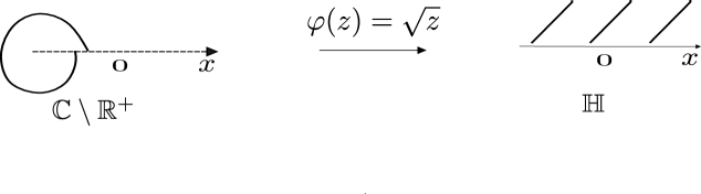
Figure 1: The map $\varphi$

We know that $f^{k}(q)$ will always be on the negative real axis for any integer $k\geq 0$. We choose $\theta_{0}>0$ and two rays $l_{1}:=\{z=re^{i\theta_{0}},r>0\},l_{2}:=\{z=re^{-i\theta_{0}},r>0\}$. Then we denote by $T:=\{z=re^{i\theta},r>0,\theta_{0}\leq\theta\leq 2\pi-\theta_{0}\}$, a sector inside $\mathbb{C}\setminus{\mathbb{R}}^{+}$.

Before continuing with the proof of Theorem A, we have the following well-known Lemma 3.2. For the reader’s convenience and to introduce notation, we include the proof and define a Left/Right Pac-Man for an easy explanation of the proof.

Definition 3.1.

We call a domain $D_{R}:=\{z=re^{i\theta},0<r\leq R,\theta_{0}<\theta<2\pi-\theta_{0}\}$ a Left Pac-Man and $\tilde{D}_{R}:=\{z=re^{i\theta},0<r\leq R,-\pi+\theta_{0}<\theta<\pi-\theta_{0}\}$ a Right Pac-Man.

Lemma 3.2.

There exists a Left Pac-Man $D_{R_{0}}$ such that $D_{R_{0}}\subsetneqq T\cap\mathcal{A}.$

Proof.

We want to know how orbits go precisely near the parabolic fixed point at $0.$ Let $\omega=\varphi(z)=-1/z$ send $0$ to $\infty,$ then the conjugated map has the expansion

$$F(\omega)=\varphi\circ f\circ\varphi^{-1}(\omega)=\omega+1+o(1)~{}~{}\text{as}~{}~{}|\omega|\rightarrow\infty.$$

And we have $l_{1}(l_{2})$ is mapped to two new rays $l^{\omega}_{1}:=\{z=re^{i(\pi-\theta_{0})},r>0\}(l^{\omega}_{2}:=\{z=re^{i(-\pi+\theta_{0})}\})$; $T$ is mapped to $T^{\prime}=\{re^{i\theta},r>0,-\pi+\theta_{0}\leq\theta\leq\pi-\theta_{0}\}$; the Left Pac-Man $D_{R}$ is mapped to $T^{\prime}\setminus\tilde{D}_{\frac{1}{R}}$ for any radius $R$ (see Figure 2).

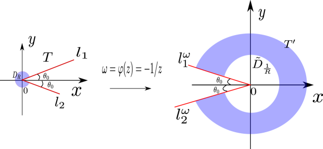
Figure 2: The image of a Left Pac-Man

We choose a Right Pac-Man $\tilde{D}_{\frac{1}{r_{0}}}$ such that for any $\omega\in T^{\prime}\setminus\tilde{D}_{\frac{1}{r_{0}}},$ we have $|o(1)|<\frac{\theta_{0}}{3}$. Note here, actually, $r_{0}=r_{0}(\theta_{0})$ should be sufficiently small. Then we draw the upper tangent line $L_{0}$ of $\tilde{D}_{\frac{1}{r_{0}}}$ such that the angle between $L_{0}$ and the real axis is $\frac{\theta_{0}}{2}$. Then $L_{0}$ will intersect $l_{1}^{\omega}$ and the real axis, we denote these two intersect points $A_{0}$ and $B_{0},$ respectively. Let $\frac{1}{r}=\max\{|OA_{0}|,|OB_{0}|\}>\frac{1}{r_{0}}$, here $O$ is the origin zero, then we choose the Right Pac-Man $\tilde{D}_{\frac{1}{r}}$ (see Figure 3).

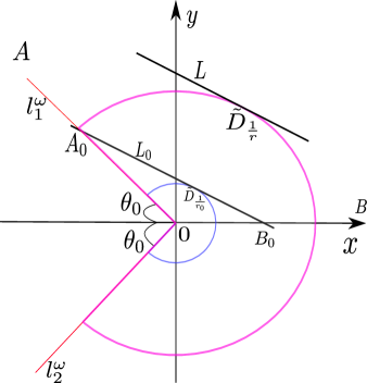
Figure 3: The choice of the Right Pac-Man

If we take any $\omega_{0}\in T^{\prime}\setminus\tilde{D}_{\frac{1}{r}}$, $F^{n}(\omega_{0})=\omega_{0}+n+o(1)$ for all positive integers $n$ such that $|F^{n}(\omega_{0})|\geq|\omega_{0}+n-n\frac{\theta_{0}}{3}|$, then we know that $F^{n}(\omega_{0})$ will never go inside $\tilde{D}_{\frac{1}{r_{0}}}.$

Therefore, let $R_{0}=r,\tilde{R}_{0}=r_{0},$ then we have for any $z_{0}\in D_{R_{0}},f^{n}(z_{0})\rightarrow 0,$ hence $D_{R_{0}}\subsetneqq T\cap\mathcal{A},$ and we also know that $f^{n}(D_{R_{0}})\subseteq D_{\tilde{R}_{0}}.$

∎

Lemma 3.3.

We can choose a Left Pac-Man $D_{R^{\prime}_{0}}\subseteq D_{R_{0}}$ such that $f^{n}(D_{R^{\prime}_{0}})\subseteq D_{R_{0}}$ for all $n=1,2,\dots$

Proof.

On the procedure for proving Lemma 3.2, we can draw another upper tangent line $L$ of $\tilde{D}_{R_{0}}$ such that the angle between $L$ and the real axis is $\frac{\theta_{0}}{2}$. Then $L$ will also intersect $l_{1}^{\omega}$ and the real axis, we denote these two intersect points $A$ and $B$ respectively. Let $\frac{1}{r^{\prime}}=\max\{|OA|,|OB|\}$, then we choose the Right Pac-Man $\tilde{D}_{\frac{1}{r^{\prime}}}.$ If we take any $\omega\in T^{\prime}\setminus\tilde{D}_{\frac{1}{r^{\prime}}}$, we know that $F^{n}(\omega)$ will never go inside of $\tilde{D}_{\frac{1}{r}}.$ Hence, let $R^{\prime}_{0}=\frac{1}{r^{\prime}},$ we have $f^{n}(D_{R^{\prime}_{0}})\subseteq D_{R_{0}}.$

∎

We continue with the proof of Theorem A. The idea of the proof is to find a point $z_{0}\in D_{\varepsilon}\setminus{\mathbb{R}}^{-}$ such that for any $\tilde{q}\in Q,$ we have $d_{\mathcal{A}}(z_{0},\tilde{q})\geq C$.

Now, we will consider the following cases of $\tilde{q}$ inside three subsets of $\mathcal{A}$ (see Figure 4):

Case 1: $\tilde{q}\in\big{(}(T\cap\mathcal{A})\setminus D_{R^{\prime}_{0}}\big{)}\setminus{\mathbb{R}}^{-}.$ Let $d^{1}_{\mathcal{A}}(z_{0},\tilde{z})$ be the Kobayashi distance between $z_{0}$ and any point $\tilde{z}\in\partial D_{R^{\prime}_{0}}\setminus R^{-}$ (see the blue curve in Figure 4). Then we prove that $d^{1}_{\mathcal{A}}(z_{0},\tilde{z})\geq C$.

Case 2: $\tilde{q}\in{\mathbb{R}}^{-}.$ Let $d^{2}_{\mathcal{A}}(z_{0},z^{\prime})$ be the Kobayashi distance between $z_{0}$ and any point $z^{\prime}\in{\mathbb{R}}^{-}\cap\mathcal{A}$ (see the pink curve in Figure 4). Then we prove that $d^{2}_{\mathcal{A}}(z_{0},z^{\prime})\geq C$.

Case 3: $\tilde{q}\in\mathcal{A}\cap\big{\{}S^{\prime}:=\{z=re^{i\theta},r>0,0<\theta\leq\theta_{0}\}\big{\}}.$ Let $d^{3}_{\mathcal{A}}(z_{0},\hat{z})$ be the Kobayashi distance between $z_{0}$ and any point $\hat{z}\in l_{1}$ (see the green curve in Figure 4). Then we prove that $d^{3}_{\mathcal{A}}(z_{0},\hat{z})\geq C$.

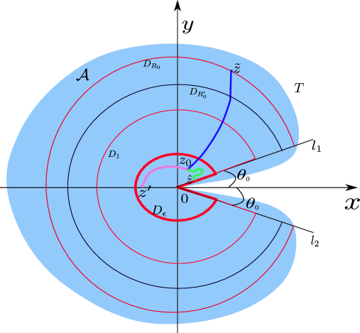
Figure 4: The three Kobayashi distances in $\mathcal{A}$

Remark:

1) In the investigation of these three cases, it will become clear how small $\theta_{0}$ needs to be.

2) $\partial D_{R^{\prime}_{0}}$ means the boundary of the Left Pac-Man $D_{R^{\prime}_{0}}.$ It is the circular curve of $D_{R^{\prime}_{0}},$ not including the mouth of $D_{R^{\prime}_{0}}$ which belongs to $l_{1}$ and $l_{2};$

3) $\tilde{q}$ can never be inside $D_{R^{\prime}_{0}}\setminus{\mathbb{R}}^{-}:$ If $\tilde{q}\in D_{R^{\prime}_{0}}\setminus{\mathbb{R}}^{-},$ more precisely, suppose $f^{-l}(f^{k}(q))\in D_{R^{\prime}_{0}}\setminus{\mathbb{R}}^{-}$ for some integers $l,k\geq 0,$ we iterate $l$ times of $f^{-l}(f^{k}(q))$, we have $f^{k}(q)\in D_{R_{0}}\setminus{\mathbb{R}}^{-}$ since we know $f^{n}(D_{R^{\prime}_{0}})\subseteq D_{R_{0}}$ for any positive integer $n$ by Lemma 3.2 and $f^{k}(q)\notin{\mathbb{R}}^{-}$ since $R^{\prime}_{0}<R_{0}=r<r_{0}$, and $f$ is biholomorphic near $0.$ Hence $\operatorname{Im}(f^{k}(q))\neq 0$. However, this contradicts $\operatorname{Im}(f^{k}(q))=\operatorname{Im}(f^{k}(-\frac{1}{2}))=0.$ Thus $\tilde{q}\notin D_{R^{\prime}_{0}}\setminus{\mathbb{R}}^{-};$

4) if $\tilde{q}\in\mathcal{A}\setminus D_{R^{\prime}_{0}},$ $\tilde{q}$ is far away from $\partial D_{R^{\prime}_{0}}$, then we know that $d_{\mathcal{A}}(z_{0},\tilde{q})\geq d^{1}_{\mathcal{A}}(z_{0},\tilde{z})$. This is because $d^{1}_{\mathcal{A}}(z_{0},\tilde{z})$ is the minimum distance between $z_{0}$ and any $\tilde{q}\in\big{(}(T\cap\mathcal{A})\setminus D_{R^{\prime}_{0}}\big{)}\setminus{\mathbb{R}}^{-}.$

Hence, we need to prove that we can choose $z_{0}$ so that all these three Kobayashi distances $d^{1}_{\mathcal{A}}(z_{0},\tilde{z}),d^{2}_{\mathcal{A}}(z_{0},z^{\prime}),d^{3}_{\mathcal{A}}(z_{0},\hat{z})\geq C$ for the given constant $C$. Next, we will estimate these three Kobayashi distances.

First, we estimate $d^{1}_{\mathcal{A}}(z_{0},\tilde{z}).$ Suppose $z_{0}\in D_{\varepsilon},$

$$d^{1}_{\mathcal{A}}(z_{0},\tilde{z})\geq d_{\mathbb{C}\setminus{\mathbb{R}}^{+}}(z_{0},\tilde{z})$$

$$= \inf\int_{\gamma(t)}F_{\mathbb{C}\setminus{\mathbb{R}}^{+}}(\gamma(t))|\gamma^{\prime}(t)|dt$$

$$= \inf\int_{\gamma(t)}\frac{1}{2|\gamma(t)|\sin\frac{\arg(\gamma(t))}{2}}|\gamma^{\prime}(t)|dt$$

$$\geq \inf\int_{\gamma(t)}\frac{1}{2|\gamma(t)|}|\gamma^{\prime}(t)|dt$$

$$= \frac{1}{2}\inf\int_{\varepsilon}^{R^{\prime}_{0}}\frac{|dr|}{r}$$

$$\geq \frac{1}{2}(\ln R^{\prime}_{0}-\ln\varepsilon),$$

where $\gamma(t)$ is a smooth path joining $z_{0}$ to $\tilde{z}$. The last inequality holds since there might have some derivatives of the path $\gamma(t)$ are negative in some pieces. In addition, we can see that $d^{1}_{\mathcal{A}}(z_{0},\tilde{z})\rightarrow\infty$ as $\varepsilon\rightarrow 0.$

Second, we estimate $d^{2}_{\mathcal{A}}(z_{0},z^{\prime})$. Let $\varepsilon=\varepsilon_{0}$, i.e., fix $\varepsilon,$ and let $D_{1}\subset T$ be a scaling of $D_{\varepsilon_{0}}$ by $S(z)=\frac{z}{|z_{0}|},$ sending $z_{0},z^{\prime}$ to $\tilde{z}_{0}:=\frac{z_{0}}{|z_{0}|},\frac{z^{\prime}}{|z_{0}|}$, respectively. By homogeneity, we know the Kobayashi distance $d_{\mathbb{C}\setminus{\mathbb{R}}^{+}}(z_{0},z^{\prime})=d_{\mathbb{C}\setminus{\mathbb{R}}^{+}}(\tilde{z}_{0},z^{\prime}/|z_{0}|)$. Since we hope to prove $d^{2}_{\mathcal{A}}(z_{0},z^{\prime})\geq C$, we need $z_{0}$ to be far from $\mathbb{R}^{-}$, and so does $\tilde{z}_{0}$. Let $S_{T}:=\{z=e^{i\theta},\theta_{0}<\theta<\frac{\pi}{2}-\theta_{0}\}$, assume $\tilde{z}_{0}\in S_{T}$ and $\operatorname{Re}\tilde{z}_{0}>\frac{1}{2}$, then any curve from $\tilde{z}_{0}$ to $\frac{z^{\prime}}{|z_{0}|}$ must pass through a point $\tilde{z}^{\prime}$ on the positive imaginary axis, i.e., $\operatorname{Re}\tilde{z}^{\prime}=0$. For simplicity, we assume this curve and $\tilde{z}^{\prime}$ lie in the upper half plane. Hence $d^{2}_{\mathcal{A}}(z_{0},z^{\prime})\geq d_{\mathbb{C}\setminus{\mathbb{R}}^{+}}(z_{0},z^{\prime})=d_{\mathbb{C}\setminus{\mathbb{R}}^{+}}(\tilde{z}_{0},z^{\prime}/|z_{0}|)\geq d_{\mathbb{C}\setminus{\mathbb{R}}^{+}}(\tilde{z}_{0},\tilde{z}^{\prime}).$ We have

$$d^{2}_{\mathcal{A}}(z_{0},z^{\prime}) \geq d_{\mathbb{C}\setminus{\mathbb{R}}^{+}}(\tilde{z}_{0},\tilde{z}^{\prime})$$

$$=\inf\int_{\tilde{z}_{0}}^{\tilde{z}^{\prime}}F_{\mathbb{C}\setminus{\mathbb{R}}^{+}}(z)$$

$$=\inf\int_{\tilde{z}_{0}}^{\tilde{z}^{\prime}}\frac{|dz|}{|z|2\sin(\theta/2)}$$

$$\geq\sqrt{2}\inf\int_{\tilde{z}_{0}}^{\tilde{z}^{\prime}}\frac{|dz|}{|z|\sin\theta}$$

$$\geq\sqrt{2}\inf\int_{\tilde{z}_{0}}^{\tilde{z}^{\prime}}\frac{|dz|}{\operatorname{Im}z}$$

$$>\sqrt{2}|\ln(\operatorname{Im}\tilde{z}^{\prime})-\ln(\operatorname{Im}\tilde{z}_{0})|.$$

Then there are three situations for the Kobayashi distance between $\tilde{z}_{0}$ and $\tilde{z}^{\prime}:$

1) If $\operatorname{Im}\tilde{z}^{\prime}\geq e^{C}|\operatorname{Im}\tilde{z}_{0}|$ or $\operatorname{Im}\tilde{z}^{\prime}\leq\frac{|\operatorname{Im}\tilde{z}_{0}|}{e^{C}}$ for the constant $C>0$ (see the blue curves on Figure 5), then $|\ln(\operatorname{Im}\tilde{z}^{\prime})-\ln(\operatorname{Im}\tilde{z}_{0})|\geq C,$ hence $d^{2}_{\mathcal{A}}(z_{0},z^{\prime})\geq C$ is true.

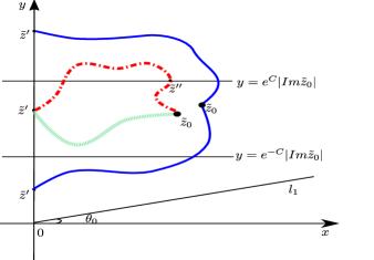
Figure 5: Three situations for the Kobayashi distance between $\tilde{z}_{0}$ and $\tilde{z}^{\prime}$

2) lf $\tilde{z}^{\prime}\in\mathcal{L}:=\{z=x+iy,\frac{|\operatorname{Im}\tilde{z}_{0}|}{e^{C}}<y<e^{C}|\operatorname{Im}\tilde{z}_{0}|\}$ (see the green curve on Figure 5). We prove that $d_{\mathcal{A}}(\tilde{z}_{0},\tilde{z}^{\prime})\geq\sqrt{2}\inf\int_{\tilde{z}_{0}}^{\tilde{z}^{\prime}}\frac{|dz|}{\operatorname{Im}z}\geq C$ for $z\in\mathcal{L}$.

Let $z=x+iy\in\mathcal{L}$, then $\operatorname{Im}z\leq e^{C}|\operatorname{Im}\tilde{z}_{0}|$. Hence we have

$$\int_{\tilde{z}_{0}}^{\tilde{z}^{\prime}}\frac{|dz|}{\operatorname{Im}z}\geq\int_{\tilde{z}_{0}}^{\tilde{z}^{\prime}}\frac{|dx|}{\operatorname{Im}z}\geq\int_{\tilde{z}_{0}}^{\tilde{z}^{\prime}}\frac{|dx|}{e^{C}|\operatorname{Im}\tilde{z}_{0}|}=\frac{\operatorname{Re}\tilde{z}_{0}}{e^{C}}\frac{1}{|\operatorname{Im}\tilde{z}_{0}|}>\frac{1}{2e^{C}|\operatorname{Im}\tilde{z}_{0}|}.$$

Note that the last inequality holds because we choose $\operatorname{Re}\tilde{z}_{0}>1/2.$

As long as $\theta_{0}<\frac{1}{2Ce^{C}}$, we can choose $\tilde{z}_{0}$ so that $\operatorname{Im}\tilde{z}_{0}<\frac{1}{2Ce^{C}}$, hence $\int_{\tilde{z}_{0}}^{\tilde{z}^{\prime}}\frac{|dz|}{\operatorname{Im}z}>C.$

3) If $\tilde{z}^{\prime}\in\mathcal{L},$ but the curve $\gamma$ between $\tilde{z}_{0}$ and $\tilde{z}^{\prime}$ gets outside of $\mathcal{L}$ starting at some point $\tilde{z}^{\prime\prime}\in\gamma\cap\mathcal{L}$ for a while (see the red curve in Figure 5), then enter back to $\mathcal{L}$ again, then we still have $d^{2}_{\mathcal{A}}(z_{0},z^{\prime})\geq C$ is true because $d_{\mathbb{C}\setminus{\mathbb{R}}^{+}}(z_{0},z^{\prime})\geq d_{\mathbb{C}\setminus{\mathbb{R}}^{+}}(\tilde{z}_{0},\tilde{z}^{\prime\prime})\geq C.$ The last inequality holds since 1) is valid.

After these calculations, we fix $z_{0}$ so that $d^{1}_{\mathcal{A}}(z_{0},\tilde{z})$ and $d^{2}_{\mathcal{A}}(z_{0},z^{\prime})$ are both bigger or equal to $C.$ To obtain $d^{3}_{\mathcal{A}}(z_{0},\hat{z})\geq C,$ we will need an even smaller $\theta^{\prime}_{0},$ see the following calculation.

We know $d^{3}_{\mathcal{A}}(z_{0},\hat{z})\geq d_{\mathbb{C}\setminus{\mathbb{R}}^{+}}(z_{0},\hat{z})=d_{\mathbb{C}\setminus{\mathbb{R}}^{+}}(\tilde{z}_{0},\hat{z}/|z_{0}|).$ Hence to have $d^{3}_{\mathcal{A}}(z_{0},\hat{z})\geq C,$ we need to estimate $d_{\mathbb{C}\setminus{\mathbb{R}}^{+}}(\tilde{z}_{0},\hat{z}/|z_{0}|).$

When we estimate $d^{2}_{\mathcal{A}}(z_{0},z^{\prime})$, we send $z_{0}$ to $\tilde{z}_{0}$ and choose $\operatorname{Re}\tilde{z}_{0}>1/2$ and $\tilde{z}$ close to $l_{1}.$ Hence $d_{\mathbb{C}\setminus{\mathbb{R}}^{+}}(\tilde{z}_{0},\hat{z}/|z_{0}|)$ might be very small. To handle this situation, we first choose a disk $\Delta^{K}_{\mathbb{C}\setminus{\mathbb{R}}^{+}}(\tilde{z}_{0},C)$ centered at $\tilde{z}_{0}$ with Kobayashi radius $C$. Since this disk $\Delta^{K}_{\mathbb{C}\setminus{\mathbb{R}}^{+}}(\tilde{z}_{0},C)$ is a compact subset of $\mathbb{C}\setminus{\mathbb{R}}^{+}$, there exists a sector $S^{\prime\prime}:=\{z=re^{i\theta},r>0,0<\theta<\theta^{\prime}_{0}\}$ such that $S^{\prime\prime}\cap\Delta^{K}_{\mathbb{C}\setminus{\mathbb{R}}^{+}}(\tilde{z}_{0},C)=\emptyset$, here we can assume that $\theta^{\prime}_{0}<\theta_{0}.$ Therefore, $d_{\mathbb{C}\setminus{\mathbb{R}}^{+}}(\tilde{z}_{0},\hat{z}/|z_{0}|)\geq C$ for any $\hat{z}/|z_{0}|\in\mathcal{A}\cap S^{\prime\prime}.$ Furthermore, for this new $\theta^{\prime}_{0},$ it does not change the conclusion of the estimation of $d^{1}_{\mathcal{A}}(z_{0},\tilde{z})$ and $d^{2}_{\mathcal{A}}(z_{0},z^{\prime}).$

Therefore, there is a point $z_{0}$ such that all these three distances $d^{1}_{\mathcal{A}}(z_{0},\tilde{z}),d^{2}_{\mathcal{A}}(z_{0},z^{\prime}),d^{3}_{\mathcal{A}}(z_{0},\hat{z})\geq C$ for the given constant $C.$

∎

3.2 Dynamics inside the parabolic basin of $f(z)=z+az^{m+1},m\geq 1,a\neq 0$

In this subsection, we generalize Theorem A to the case of several petals inside the parabolic basin. Let us recall the statement of our main Theorem B:

Theorem B.

Let $f(z)=z+az^{m+1},m\geq 1,a\neq 0$, and $\Omega_{j}$ be the immediate basin of $\mathcal{A}_{j}.$ We choose an arbitrary constant $C>0$ and a point $q\in{\bf v_{j}}\cap\mathcal{P}_{j}$. Then there exists a point $z_{0}\in\Omega_{j}$ so that for any $\tilde{q}\in Q:=(\cup_{l=0}^{\infty}f^{-l}(f^{k}(q)))\cap\Omega_{j}~{}(l,k$ are non-negative integers), the Kobayashi distance $d_{\Omega_{j}}(z_{0},\tilde{q})\geq C$, where $d_{\Omega_{j}}$ is the Kobayashi metric.

Proof.

Let $S:=\{z=re^{i\theta},r>0,0<\theta<\frac{2\pi}{m}\}$ be the sector with angle $2\pi/m$, including the attracting petal $\mathcal{P}_{j}$, then the angle between ${\bf v_{j}}$ and ${\mathbb{R}}^{+}$ is $\frac{\pi}{m}$. We denote the boundary rays of $S$ by $l^{1}_{{\mathbb{R}}^{+}}:=\{z=r>0\}$ and $l^{2}_{{\mathbb{R}}^{+}}:=\{z=re^{i\frac{2\pi}{m}},r>0\}$. We choose $\theta_{0}>0$ and two rays $l_{1}:=\{z=re^{i\theta_{0}},r>0\},l_{2}:=\{z=re^{i(\frac{2\pi}{m}-\theta_{0})},r>0\}$. Then we denote by $T:=\{z=re^{i\theta},r>0,\theta_{0}<\theta<\frac{2\pi}{m}-\theta_{0}\}$ a sector inside $S.$

Let $\varphi(z):S\rightarrow\mathbb{H}$ with $\varphi(z)=z^{m/2}$. Then the Kobayashi metric $F_{S}$ is

$$F_{S}=\frac{|\varphi^{\prime}|}{\operatorname{Im}\varphi}|dz|=\frac{m}{2r\sin(\frac{\theta m}{2})}|dz|.$$

As in the proof of Theorem A, we can choose two analogous ”Pac-Man” $D^{m}_{R^{\prime}_{0}}:=\{z=re^{i\theta},0<r<R^{\prime}_{0},\theta_{0}<\theta<\frac{2\pi}{m}-\theta_{0}\},D^{m}_{R_{0}}:=\{z=re^{i\theta},0<r<R_{0},\theta_{0}<\theta<\frac{2\pi}{m}-\theta_{0}\}$ central at $0$ with radius $R^{\prime}_{0},R_{0}>0(R^{\prime}_{0}<R_{0})$, respectively, such that $D^{m}_{R_{0}}\subsetneqq T\cap\Omega_{j}$ and $f^{n}(D^{m}_{R^{\prime}_{0}})\subset D^{m}_{R_{0}}.$ Then similarly, we need to estimate the three Kobayashi distances from $z_{0}$ to any point $\tilde{z}\in\partial D^{m}_{R_{0}}$ (see the blue curve in Figure 6), $z^{\prime}\in{\bf v_{j}}$ (see the pink curve in Figure 6), and $\hat{z}\in\Omega_{j}\cap\big{\{}S^{\prime}:=\{z=re^{i\theta},r>0,0<\theta<\theta_{0}\}\big{\}}$ (see the green curve in Figure 6), and show that all of them are not less than $C$.

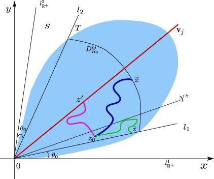
Figure 6: The three Kobayashi distances in $\Omega_{j}$

First, suppose $z_{0}\in D^{m}_{\varepsilon}:=\{z=re^{i\theta},0<r<\varepsilon,\theta_{0}<\theta<\frac{2\pi}{m}-\theta_{0}\},\varepsilon<<R^{\prime}_{0}.$ Let us estimate the Kobayashi distance from $z_{0}$ to any point $\tilde{z}$ on the boundary of $D^{m}_{R_{0}}$, and we denote this distance by $d^{1}_{\Omega_{j}}(z_{0},\tilde{z}).$

$$d^{1}_{\Omega_{j}}(z_{0},\tilde{z}) \geq d_{S}(z_{0},\tilde{z})=\inf\int_{\gamma(t)}F_{S}(\gamma(t))|\gamma^{\prime}(t)|dt$$

$$=\inf\int_{\gamma(t)}\frac{m}{2|\gamma(t)|\sin\frac{m\arg(\gamma(t))}{2}}|\gamma^{\prime}(t)|dt\geq\inf\int_{\gamma(t)}\frac{m}{2|\gamma(t)|}|\gamma^{\prime}(t)|dt$$

$$=\frac{m}{2}\inf\int_{\varepsilon}^{R_{0}}\frac{|dr|}{r}\geq\frac{m}{2}(\ln R_{0}-\ln\varepsilon),$$

where $\gamma(t)$ is a smooth path joining $z_{0}$ to $\tilde{z}$. In addition, we can see that $d^{1}_{\Omega_{j}}(z_{0},\tilde{z})\rightarrow\infty$ as $\varepsilon\rightarrow 0.$

Second, we calculate the Kobayashi distance from $z_{0}$ to any point $z^{\prime}\in{\bf v_{j}}$ denoted by $d^{2}_{\Omega_{j}}(z_{0},z^{\prime})$. Let $\varepsilon=\varepsilon_{0}$, i.e., fix $\varepsilon,$ and $D^{m}_{1}\subset T$ be a scaling of $D^{m}_{\varepsilon_{0}}$ by $S(z)=\frac{z}{|z_{0}|}$, sending $z_{0},z^{\prime}$ to $\tilde{z}_{0}:=\frac{z_{0}}{|z_{0}|},\frac{z^{\prime}}{|z_{0}|}$, respectively. By homogeneity, we know the Kobayashi distance $d_{S}(z_{0},z^{\prime})=d_{S}(\tilde{z}_{0},z^{\prime}/|z_{0}|)$. Since we hope to prove $d^{2}_{\Omega_{j}}(z_{0},z^{\prime})>C$, we need $z_{0}$ to be far from ${\bf v_{j}}$, and so does $\tilde{z}_{0}$. Let $S_{T}:=\{z=e^{i\theta},\theta_{0}<\theta<\frac{\pi}{2m}-\theta_{0}\}$, assume $\tilde{z}_{0}\in S_{T}$ and $\operatorname{Re}\tilde{z}_{0}$ is sufficiently big, then any curve from $\tilde{z}_{0}$ to $\frac{z^{\prime}}{|z_{0}|}$ must pass through a point $\tilde{z}^{\prime}$ on the ray $Y^{+}:=\{re^{i\frac{\pi}{2m}},r>0\}.$ Hence $d^{2}_{\Omega_{j}}(z_{0},z^{\prime})\geq d_{S}(z_{0},z^{\prime})=d_{S}(\tilde{z}_{0},z^{\prime}/|z_{0}|)\geq d_{S}(\tilde{z}_{0},\tilde{z}^{\prime}).$ Then we have

$$d^{2}_{\Omega_{j}}(z_{0},z^{\prime}) \geq d_{S}(\tilde{z}_{0},\tilde{z}^{\prime})=\inf\int_{\tilde{z}_{0}}^{\tilde{z}^{\prime}}F_{S}(z)$$

$$=\inf\int_{\tilde{z}_{0}}^{\tilde{z}^{\prime}}\frac{m|dz|}{2r\sin(m\theta/2)}$$

$$=\inf\int_{\tilde{z}_{0}}^{\tilde{z}^{\prime}}\frac{\frac{m\theta}{2}}{\sin(\frac{m\theta}{2})}\cdot\frac{m|dz|}{2r(m\theta/2)}$$

$$=c_{1}\inf\int_{\tilde{z}_{0}}^{\tilde{z}^{\prime}}\frac{|dz|}{r\theta}$$

$$=c_{1}\inf\int_{\tilde{z}_{0}}^{\tilde{z}^{\prime}}\frac{\sin\theta}{\theta}\cdot\frac{|dz|}{r\sin\theta}$$

$$=c_{1}c_{2}\inf\int_{\tilde{z}_{0}}^{\tilde{z}^{\prime}}\frac{|dz|}{r\sin\theta}$$

$$=c_{1}c_{2}\inf\int_{\tilde{z}_{0}}^{\tilde{z}^{\prime}}\frac{|dz|}{\operatorname{Im}z}$$

$$\geq c_{1}c_{2}|\ln(\operatorname{Im}\tilde{z}^{\prime})-\ln(\operatorname{Im}\tilde{z}_{0})|.$$

where $c_{1}:=\inf\frac{\frac{m\theta}{2}}{\sin\frac{m\theta}{2}},c_{2}:=\inf\frac{\sin\theta}{\theta}.$

Then there are three situations for the Kobayashi distance between $\tilde{z}_{0}$ and $\tilde{z}^{\prime}:$

1) If $\operatorname{Im}\tilde{z}^{\prime}\geq e^{C}|\operatorname{Im}\tilde{z}_{0}|$ or $\operatorname{Im}\tilde{z}^{\prime}\leq\frac{|\operatorname{Im}\tilde{z}_{0}|}{e^{C}}$ for some constant $C>1$, then $|\ln(\operatorname{Im}\tilde{z}^{\prime})-\ln(\operatorname{Im}\tilde{z}_{0})|\geq C,$ hence $d^{2}_{\Omega_{j}}(z_{0},z^{\prime})\geq C$ is true.

2) lf $\tilde{z}^{\prime}\in\mathcal{L}:=\{z=x+iy,\frac{|\operatorname{Im}\tilde{z}_{0}|}{e^{C}}<y<e^{C}|\operatorname{Im}\tilde{z}_{0}|\}$. We need to prove that $d_{\Omega_{j}}(\tilde{z}_{0},\tilde{z}^{\prime})\geq c_{1}c_{2}\inf\int_{\tilde{z}_{0}}^{\tilde{z}^{\prime}}\frac{|dz|}{\operatorname{Im}z}\geq C$ for $z\in\mathcal{L}$.

Let $z=x+iy\in\mathcal{L}$, then $\operatorname{Im}z\leq e^{C}|\operatorname{Im}\tilde{z}_{0}|$. Hence we have

$$\int_{\tilde{z}_{0}}^{\tilde{z}^{\prime}}\frac{|dz|}{\operatorname{Im}z}\geq\int_{\tilde{z}_{0}}^{\tilde{z}^{\prime}}\frac{|dx|}{\operatorname{Im}z}\geq\int_{\tilde{z}_{0}}^{\tilde{z}^{\prime}}\frac{|dx|}{e^{C}|\operatorname{Im}\tilde{z}_{0}|}=\frac{|\operatorname{Re}\tilde{z}^{\prime}-\operatorname{Re}\tilde{z}_{0}|}{e^{C}}\frac{1}{|\operatorname{Im}\tilde{z}_{0}|}>\frac{1}{2e^{C}|\operatorname{Im}\tilde{z}_{0}|},$$

Note that the last inequality holds since we choose $\operatorname{Re}\tilde{z}_{0}$ sufficiently big so that $\tilde{z}_{0}$ is close to $l_{1}$, and $|\operatorname{Re}\tilde{z}^{\prime}-\operatorname{Re}\tilde{z}_{0}|>1/2$ because $\tilde{z}^{\prime}$ will have to be close to $0$ since it lies on $Y^{+}\cap\mathcal{L}$ and its imaginary part is close to $0$, which makes $d^{2}_{\Omega_{j}}(z_{0},z^{\prime})$ as big as we want.

In other words, as long as $\theta_{0}<\frac{1}{2Ce^{C}}$, we have $\operatorname{Im}\tilde{z}_{0}<\frac{1}{2Ce^{C}}$. In addition, $|\operatorname{Re}\tilde{z}^{\prime}-\operatorname{Re}\tilde{z}_{0}|>1/2$, we obtain $\int_{\tilde{z}_{0}}^{\tilde{z}^{\prime}}\frac{|dz|}{\operatorname{Im}z}>C.$

3) If $\tilde{z}^{\prime}\in\mathcal{L},$ but the curve $\gamma$ between $\tilde{z}_{0}$ and $\tilde{z}^{\prime}$ get outside of $\mathcal{L}$ starting at some point $\tilde{z}^{\prime\prime}\in\gamma\cap\mathcal{L}$ for a while, then enter back to $\mathcal{L}$ again, then we still have $d^{2}_{\Omega_{j}}(z_{0},z^{\prime})\geq C$ is true because $d_{S}(z_{0},z^{\prime})\geq d_{S}(\tilde{z}_{0},\tilde{z}^{\prime\prime})\geq C.$ The last inequality holds since 1) is valid. We have a conclusion as same as $d^{2}_{\mathcal{A}}(z_{0},z^{\prime})\geq C$ in the proof of Theorem A.

At last, we estimate the Kobayashi distance from $z_{0}$ to any point $\hat{z}\in\Omega_{j}\cap\big{\{}S^{\prime}:=\{z=re^{i\theta},r>0,0<\theta<\theta_{0}\}\big{\}}$ denoted by $d^{3}_{\Omega_{j}}(z_{0},\hat{z}).$ We know $d^{3}_{\Omega_{j}}(z_{0},\hat{z})\geq d_{S}(z_{0},\hat{z})=d_{S}(\tilde{z}_{0},\hat{z}/|z_{0}|).$

We use the method for computing $d^{3}_{\Omega_{j}}(z_{0},\hat{z})$ as same as $d^{3}_{\mathcal{A}}(z_{0},\hat{z})\geq C$ in the proof of Theorem A. We first choose a disk $\Delta^{K}_{S}(\tilde{z}_{0},C)$ centered at $\tilde{z}_{0}$ with Kobayashi radius $C$. Since this disk $\Delta^{K}_{S}(\tilde{z}_{0},C)$ is a compact subset of $S$, there exists a sector $S^{\prime\prime}:=\{z=re^{i\theta},r>0,\pi-\frac{\pi}{m}<\theta<\pi-\frac{\pi}{m}+\theta^{\prime}_{0}\}$ such that $S^{\prime\prime}\cap\Delta^{K}_{S}(\tilde{z}_{0},C)=\emptyset$, here we can assume that $\theta^{\prime}_{0}<\theta_{0}.$ Therefore, $d_{S}(\tilde{z}_{0},\hat{z}/|z_{0}|)\geq C$ for any $\hat{z}/|z_{0}|\in\Omega_{j}\cap S^{\prime\prime}.$ Furthermore, for this new $\theta^{\prime}_{0},$ it does not change the conclusion of the estimation of $d^{1}_{\Omega_{j}}(z_{0},\tilde{z})$ and $d^{2}_{\Omega_{j}}(z_{0},z^{\prime}).$

∎

3.3 Dynamics inside the parabolic basin of $f(z)=z+az^{m+1}+(\text{higher terms}),m\geq 1,a\neq 0$

Finally, in this subsection, we sketch how to handle the behavior of orbits inside parabolic basins of general polynomials. Let us recall the statement of our main Theorem C:

Theorem C.

Let $f(z)=z+az^{m+1}+(\text{higher terms}),m\geq 1,a\neq 0,$ and $\Omega_{j}$ be the immediate basin of $\mathcal{A}_{j}.$ We choose an arbitrary constant $C>0$ and a point $q\in{\bf v_{j}}\cap\mathcal{P}_{j}$. Then there exists a point $z_{0}\in\Omega_{j}$ so that for any $\tilde{q}\in Q:=(\cup_{l=0}^{\infty}f^{-l}(f^{k}(q)))\cap\Omega_{j}~{}(l,k$ are non-negative integers), the Kobayashi distance $d_{\Omega_{j}}(z_{0},\tilde{q})\geq C$, where $d_{\Omega_{j}}$ is the Kobayashi metric.

The proof of Theorem B needs to be adjusted. To simplify the discussion, we consider the case $m=1:$

$$f(z)=z+z^{2}+(\text{higher terms}).$$

When there are no higher order terms, the crucial estimate of the Kobayashi metric comes from the fact that the parabolic basin is contained in $\mathbb{C}\setminus{\mathbb{R}}^{+}.$ Hence we could compare it with the Kobayashi metric on $\mathbb{C}\setminus{\mathbb{R}}^{+}.$

In the case of higher order terms, the parabolic basin might be more complicated. However, we can, instead of $\mathbb{C}\setminus\mathbb{R}^{+}$, use the double sheeted domain

$$V_{R}:=\{z=re^{i\theta},0<r<R,-\theta_{0}<\theta<2\pi+\theta_{0}\}.$$

Next, we investigate the properties of $V_{R}$ to explain why we choose the double sheeted domain $V_{R}$ as above.

Proposition 3.4.

Let $\bar{D}_{R}:=\{z=re^{i\theta},0<r<R,-\theta_{0}<\theta<\theta_{0}\}$, $\mathcal{A}$ be the whole basin of $f,S_{1}$ be the connected component of $\mathcal{A}\cap\bar{D}_{R}$ which contains $\{z=re^{i\theta_{0}},0<r<R\}$, and $S_{2}$ be the connected component of $\mathcal{A}\cap\bar{D}_{R}$ which contains $\{z=re^{-i\theta_{0}},0<r<R\}.$ Then any two pieces $S_{1},S_{2}$ (see the left of Figure 7) are disjoint in $\bar{D}_{R}$.

Proof.

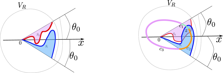
Figure 7: Two pieces $S_{1}$ and $S_{2}$ in $\bar{D}_{R}$

We know that, inside $V_{R}$ and near the origin, $\mathcal{A}$ contains the Left Pac-Man $D_{R}:=\{z=re^{i\theta},0<r<R,\theta_{0}<\theta<2\pi-\theta_{0}\}.$

If $S_{1}$ intersects $S_{2}$, then there is a point $z\in S_{1}\cap S_{2}$. We can draw three curves, $c_{1}$ from $z$ to $l_{1}:=\{z=re^{i\theta_{0}}\}$, $c_{2}$ from $z$ to $l_{2}:=\{z=re^{-i\theta_{0}}\}$, and $c_{3}\in D_{R}$ which connect $c_{1}$ and $c_{2}$. Hence $\mathcal{A}$ contains a closed curve $C:=c_{1}+c_{2}+c_{3}$ with the winding number $1$ around the origin (see the right of Figure 7).

We know that $f^{n}(z)\rightarrow 0$ when $z\in C,$ since $C\in\mathcal{A}.$ In addition, by the maximum principle, we have $f^{n}(z)\rightarrow 0$ when $z$ is inside the domain bounded by $C$. Hence $\mathcal{A}$ contains a neighborhood of $0,$ then $0$ is an attracting fixed point. However, this contradicts that $0$ is a parabolic fixed point of $f$.

∎

By Proposition 3.4, we can use the Kobayashi metric on $V_{R}$ instead of $\mathbb{C}\setminus{\mathbb{R}}^{+}$.

First, we know that $V_{R}$ can be mapped to a sector $S:=\{z=re^{i\theta},r>0,\theta_{1}<\theta<\theta_{2},\theta_{1}<<\theta_{2}<\pi/2\}$ by $\varphi_{1}(z)=z^{c/2}$ when $c$ is sufficiently small. Second, we can change $c$ such that $\theta_{2}=\pi-\theta_{1}$ by some map $\varphi_{2}(z).$ At last, by some rotation map $\varphi_{3}$, we can map $S$ to the upper half plane $\mathbb{H}$ (see the Figure 8).

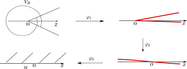
Figure 8: The maps $\varphi_{1},\varphi_{2}$ and $\varphi_{3}$

Therefore, the map $\varphi(z):=\varphi_{3}\circ\varphi_{2}\circ\varphi_{1}$ from $V$ to the upper half plane $\mathbb{H}$ becomes $\varphi(z)=e^{i\psi}z^{\frac{c}{2}}$, instead of $\varphi(z)=z^{1/2}$, where $c$ is very close to $1$. Then, with the above setting, the rest of the estimation goes through as in Theorem B.

If $m>1,$ it is difficult to draw the specific parabolic basins of $f$ or the attracting petals. Hence it is difficult to calculate the Kobayashi metric on the parabolic basin. Here we sketch the idea of how to prove this theorem for $m>1.$ We use Figure 9 to illustrate how we can choose $V_{R}$ (see the domain with pink curves as its argument), and similarly, we have the same properties of $S_{1},S_{2}$ as in Proposition 3.4 (see the red curve and blue curve on Figure 9).

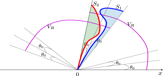
Figure 9: Two pieces $S_{1}$ and $S_{2}$

Then the rest of the estimation goes through as when $m=1$. Thus, we are done.

Corollary D.

Let $\Omega_{i,j}$ be the connected components of $\mathcal{A}_{j}$. Let $X\subset\mathcal{A}_{j}$ be the set of all $z_{0}\in\mathcal{A}_{j}$ so that $d_{\Omega_{i,j}}(z_{0},\tilde{q})\geq C$ for any $\tilde{q}$ in the same connected component $\Omega_{i,j}$ as $z_{0}$. If $z\in X,$ then any point $w\in f^{-1}(z)$ is in $X.$ Hence $X$ is dense in the boundary of $\mathcal{A}_{j}$.

Proof.

By Theorem C, we know that $X\neq\emptyset.$ Suppose $w\notin X,$ then there exists $\tilde{q}\in Q$ so that $d_{\Omega_{i,j}}(w,\tilde{q})<C$. Since $f$ is distance decreasing, see Proposition 2.7, we have $d_{\Omega_{i,j}}(f(w),f(\tilde{q}))=d_{\Omega_{i,j}}(z,f(\tilde{q}))<C.$ This contradicts $z\in X.$

Furthermore, we know that $\{f^{-n}(z)\}$ clusters at every point in Julia set. In particular, this is true if $z\in X.$ More precisely, $\{f^{-n}(z)\}$ equidistributes toward the Green measure. Therefore, $X$ is dense in the boundary of $\mathcal{A}_{j}$. ∎

References

- [1] Abate, M.: The Kobayashi distance in holomorphic dynamics and operator theory, Metrics and dynamical aspects in complex analysis, L. Blanc-Centi ed., Springer (2017)
- [2] Abate, M., Raissy, J.: Backward iteration in strongly convex domains, Adv. in Math., 228, Issue 5, 2837–2854 (2011), corrigendum (2020)
- [3] Beardon, A.F.: Iteration of Rational Functions. Springer-Verlag, New York (1991)
- [4] Bracci, F.: Speeds of convergence of orbits of non-elliptic semigroups of holomorphic self-maps of the unit disc, Ann. Univ. Mariae Curie-Sklodowska Sect. A, 73, 2, 21-43 (2019)
- [5] Bracci, F., Raissy, J., Stensønes, B.: Automorphisms of with an invariant non-recurrent attracting Fatou component biholomorphic to , JEMS, Volume 23, Issue 2, 639-666 (2021)
- [6] Brolin, H.: Invariant sets under iteration of rational functions. Ark. Mat. 6, 103-144 (1965)
- [7] Carleson, L., Gamelin, T. W.: Complex dynamics. Springer-Verlag, New York (1993)
- [8] Douady, A., Hubbard J.: tude dynamique des polynmes complexes, (Premire Partie), Publ, Math. d’Orsay 84-02 (1984); (Deuxime Partie), 85-02 (1985)
- [9] Drasin, D., Okuyama, Y.: Equidistribution and Nevanlinna theory, Bulletin of the London Mathematical Society, Volume 39, Issue 4, 603–613 (2007)
- [10] Dinh, TC., Sibony, N.: Equidistribution speed for endomorphisms of projective spaces. Math. Ann. 347, 613–626 (2010)
- [11] Fatou, P.: quations fonctionnelles, Bull. Soc. Math. France, 47, 161-271 (1919); 48, 33-94 (1920)
- [12] Hu, M.: Interior Dynamics of Fatou Sets. Preprint, available online at https://doi.org/10.48550/arXiv.2208.00546 (2022)
- [13] Krantz, S.: The Caratheodory and Kobayashi Metrics and Applications in Complex Analysis, The American Mathematical Monthly, 115, 304-329 (2008)
- [14] Milnor, J.: Dynamics in One Complex Variable. Princeton University Press, Princeton (2006)
- [15] Roesch, P., Yin, Y. Bounded critical Fatou components are Jordan domains for polynomials. Sci. China Math. 65, 331–358 (2022)
- [16] Sullivan, D.: Quasiconformal Homeomorphisms and Dynamics I. Solution of the Fatou-Julia Problem on Wandering Domains, Annals of Mathematics, Second Series, Vol. 122, No. 2, 401-418 (1985)