Sparse semiparametric discriminant analysis for high-dimensional zero-inflated data
Abstract
Sequencing-based technologies provide an abundance of high-dimensional biological datasets with skewed and zero-inflated measurements. Classification of such data with linear discriminant analysis leads to poor performance due to the violation of the Gaussian distribution assumption. To address this limitation, we propose a new semiparametric discriminant analysis framework based on the truncated latent Gaussian copula model that accommodates both skewness and zero inflation. By applying sparsity regularization, we demonstrate that the proposed method leads to the consistent estimation of classification direction in high-dimensional settings. On simulated data, the proposed method shows superior performance compared to the existing method. We apply the method to discriminate healthy controls from patients with Crohn’s disease based on microbiome data and to identify genera with the most influence on the classification rule.
Keyword: Classification; Latent Gaussian copula; Microbiome data; Probit regression; Variable selection
1 Introduction
Linear discriminant analysis (LDA) is a popular classification method due to its simple linear classification rule and Bayes optimality under the assumption that each class population is Gaussian with equal covariance matrix but different means. However, the complexity of modern high-dimensional data raises many challenges in application of classical LDA. For example, microbiome and single-cell RNA sequencing data not only contain a large number of variables relative to sample size, but also are highly skewed and zero-inflated (Silverman et al., 2020). In our motivating example of microbiome data from Vandeputte et al. (2017), we are interested in discriminating patients with Crohn’s disease from healthy controls based on genera, and identifying key genera that affect the classification rule. First, a large number of genera relative to sample size makes standard LDA suffer in terms of interpretation and accuracy, as it performs no variable selection and the sample covariance matrix becomes close to singular (Bickel and Levina, 2004). Second, the advantages of LDA under the Gaussian assumption – simple linear classification rule and Bayes optimality – can clearly not be transferred to skewed and zero-inflated data. Since LDA is very sensitive to outliers (Hastie et al., 2009), large measurement values due to skewness and large proportions of zeros can significantly bias LDA parameter estimates leading to inaccurate classification.
There is a rich body of work extending classical LDA to high-dimensional settings. A common approach is to add regularization to the classification direction vector, e.g., the regularization (Guo et al., 2007) or the regularization (Witten and Tibshirani, 2011; Mai et al., 2012; Gaynanova et al., 2016). An alternative approach is to consider data piling phenomenon in high dimensions, that is that observations from each class can be projected to a single point. Ahn and Marron (2010) estimate classification direction by maximizing the distance between data piling sites, and Lee et al. (2013) regularize the degree of data piling. While these approaches improve accuracy of LDA in the presence of larger number of variables, they still rely on assumption of Gaussian distribution, leading to poor performance in the presence of skewness and zero-inflation. Several works consider relaxations of the Gaussian assumption. Ahn et al. (2021) consider an alternative trace ratio formulation of Fisher’s LDA, which is more robust to violations of Gaussianity than standard LDA. Clemmensen et al. (2011) model each class as a mixture of Gaussian distributions with subclass-specific means and common covariance matrices. Witten (2011) and Dong et al. (2016) consider extensions of LDA model for RNA-seq data based on Poisson distribution and negative binomial distribution, respectively. Hernández and Velilla (2005) consider fully nonparametric approach with kernel LDA. Lapanowski and Gaynanova (2019) consider optimal scoring formalation of kernel LDA with sparsity regularization. These methods, although useful for high-dimensional data, are still not fully tailored for skewness and zero-inflation.
In this work, we aim to simultaneously address the issues of high-dimensionality, skewness and zero-inflation in the LDA context. We propose to achieve this by formulating a new semiparametric LDA model via the truncated latent Gaussian copula designed for zero-inflated data (Yoon et al., 2020). Latent Gaussian copula models provide an elegant framework for the analysis of non-Gaussian data of (possibly) mixed types, such as skewed continuous (Liu et al., 2009), binary (Fan et al., 2017), ordinal (Quan et al., 2018; Feng and Ning, 2019), and zero-inflated (Yoon et al., 2020). These models capture dependencies among variables via the latent correlation matrix, which can be consistently estimated by inverting a bridge function that connects latent correlations to a rank-based measure of association (Kendall’s ). Subsequently, these models have been used for graphical model estimation (Fan et al., 2017; Feng and Ning, 2019; Yoon et al., 2019) and canonical correlation analysis (Yoon et al., 2020) with non-Gaussian data. However, the use of latent Gaussian copulas in classification context has been limited. The existing approaches (Lin and Jeon, 2003; Han and Liu, 2014) are restricted to continuous data type, treating zeros as absolute. Furthermore, since standard LDA model assumes class-specific means, but the means are not identifiable under the Gaussian copula, Han et al. (2013) and Lin and Jeon (2003) enforce identifiability by enforcing marginal transformations to preserve means and variances between the observed and the latent Gaussian variables. Consequently, these approaches still rely on observation-level moment estimates, which are sensitive to zero inflation and outliers.
There are two major difficulties in adopting the truncated Gaussican copula model of Yoon et al. (2020) for LDA setting. The first difficulty is the identifiability of mean and variance parameters as described above, since the copula model is invariant under shifting and scaling of the bijective marginal transformations. Secondly, the aforementioned unsupervised problems – graphical model estimation and canonical correlation analysis – only require a consistent estimator of latent correlation matrix. In contrast, LDA encompasses both estimations of classification direction (based on latent Gaussian level) and prediction of class labels on new data (observed at non-Gaussian level), thus requiring mapping of observed data to the latent level. This is a particularly challenging task for zero-inflated data, as the mapping from observed zeros to underlying latent Gaussian variables is not one to one.
To address the identifiability difficulty, we consider a joint mixed binary-truncated copula model, where the class label is treated as dichotomized latent Gaussian variable, and zero-inflated measurements follow the truncated Gaussian copula. The joint framework encapsulates all relationships between the class label and covariates via joint latent correlation matrix. Unlike Lin and Jeon (2003); Han and Liu (2014), our approach does not require marginal transformations to be mean and variance preserving, and consequently we do not rely on observation-level moment estimates. The optimal classification direction depends only on the joint latent correlation matrix. Furthermore, by adapting -regularization, we prove that this classification direction can be estimated consistently in high-dimensional settings with the same rate as in sparse linear regression (Bickel et al., 2009). This is a non-trivial result as direct application of element-wise consistency of rank-based estimator of joint latent correlation matrix (Yoon et al., 2020) leads to suboptimal rate. To our knowledge, the closest result is obtained by Barber and Kolar (2018) for continuous Gaussian copula. However, their proof takes advantage of the closed form of the inverse bridge function. Due to significant complexity of bridge function in truncated case (Yoon et al., 2020), its inverse is not available in closed form, presenting significant new challenges for theoretical analyses.
To address the difficulty of predicting classes based on observed non-Gaussian data, we derive the posterior class probabilities conditional on observed measurements (zeros and non-zeros). We demonstrate that these probabilities can be computed using the truncated Gaussian distribution. Furthermore, we derive a Taylor approximation of the posterior probabilities that leads to a simple classification rule where the latent measurements corresponding to zeros are substituted with their conditional expectations.
In summary, our main contributions are: (a) a new LDA framework for skewed and zero-inflated data based on semiparametric mixed binary-truncated latent Gaussian copula model; (b) theoretical guarantees that the proposed framework leads to consistent estimation of classification direction in high-dimensional settings; (c) a principled approach for assigning class labels to observed zero-inflated data with non-unique mapping to latent space; (d) superior classification accuracy compared to existing methods on simulated data and microbiome data of Vandeputte et al. (2017).
The rest of the paper is organized as follows. In Section 2, we introduce the proposed classification model and describe the estimation procedures. In Section 3, we show the consistency of the estimated classification direction. In Section 4, we evaluate the classification accuracy of the proposed method with simulated datasets. In Section 5, we apply the proposed method to the quantitative microbiome dataset (Vandeputte et al., 2017) to discriminate healthy controls from patients with Crohn’s disease. In Section 6, we conclude the paper with a brief discussion.
2 Methodology
In Section 2.1, we define notations that are used throughout the paper. In Section 2.2, we propose a semiparametric linear classification model based on latent Gaussian copula after reviewing the probit regression model and its latent variable formulation. In Section 2.3, we derive the posterior probability under the proposed model and provide the Bayes classification rule.
2.1 Notation
For a vector , we denote the -norm, , by and the -norm by . For two vectors with the same size, , we write to denote element-wise inequalities such that , . For a matrix , denotes its -norm, and for a square matrix , denotes its determiant. For two matrices with the same size, , denotes the Hadamard product defined as . For two functions and , we denote their composite function by . We let denote the indicator function taking the value 1 when its argument is true and 0 otherwise. For a sequence of random variables, , we write if, for any , there exists such that for all . We let and respectively denote the -dimensional standard Gaussian distribution function with the correlation matrix evaluated at and the univariate standard Gaussian distribution function, respectively. We use to denote generic constants that do not depend on the sample size , dimension , and model parameters.
2.2 Model
Let be a random variable corresponding to class label and be a random vector of covariates. To accommodate possibly skewed and zero-inflated , we propose to model using truncated latent Gaussian copula of Yoon et al. (2020). We first review standard Gaussian copula model, which is also referred to as nonparanormal (NPN) model (Liu et al., 2009).
Definition 1 (Gaussian copula model).
A random vector satisfies the Gaussian copula model if there exist strictly increasing transformations such that , where is a correlation matrix. We write .
While Gaussian copula model can accommodate skewness through transformation functions , it does not allow zero-inflatied variables. The model of Yoon et al. (2020) allows for both zero-inflation and skewness through the following extra truncation step.
Definition 2 (Truncated Gaussian copula model).
A random vector satisfies the truncated latent Gaussian copula model if there exist a random vector and constants , , such that .
Combining the truncated Gaussian copula model for with the latent Gaussian copula model for binary variable (Fan et al., 2017) leads to the joint model for the class assignment and covariates .
Definition 3 (Latent Gaussian copula model for mixed binary-truncated data).
A random vector satisfies the latent Gaussian copula model for mixed binary-truncated data if there exist a random vector and constants , , such that
| (1) |
A special case is , , in which follows standard Gaussian copula (without truncation). Thus model (1) can also be used in binary classification settings with skewed (not necessarily zero-inflated) .
The Bayes classification rule assigns a new observation to class 1 if , and to class 0, otherwise. In the model (1), the class label depends on the covariates through underlying joint latent correlation matrix . Due to the latent Gaussian layer, the conditional probability under the model (1) is closely connected to probit regression model as we demonstrate below.
2.3 Classification rule
The probit regression model is given by , where and are the intercept and regression coefficient, respectively. Under this model, the Bayes classifier is We show that the Bayes classifier under the model (1) takes a similar form with appropriate choices of and .
First, consider the special case, where , ; that is, follows standard Gaussian copula (without truncation). By the definition, there exists latent Gaussian vector such that , , and . Let . Since ’s are strictly increasing, it follows that
Divide the correlation matrix into blocks corresponding to the latent and covariates so that and . By properties of the multivariate Gaussian distribution, , where and . Hence,
Accordingly, since , we have the same linear Bayes classifier as the probit model, with and .
Now, consider the general truncated case of model (1). Then with , . For a new vector of covariates , let and be the subvectors with truncated and observed realizations, respectively, where . Likewise, let and be the corresponding latent Gaussian vectors, and and be the corresponding threshold vectors. Then it follows that
Since as before, the posterior probability can be written as
| (2) |
where the expectation is over the multivariate Gaussian distribution of given truncated to the region . If the expectation (2) is larger than 0.5, the Bayes classification rule assigns a new observation to class 1, otherwise it assigns it to class 0.
Unfortunately, the expectation above has no closed form. We propose two approaches to address this difficulty as follows. First, we can sample from the multivariate truncated Gaussian distribution and approximate the posterior probability using the Monte-Carlo method as
| (3) |
where , is an independent sample from the -variate truncated Gaussian. This approach, however, is computationally demanding, and makes the classification rule dependent on the scaling factor (recall that the classification rules of probit and standard Gaussian copula model do not depend on ). As an alternative, we consider the first-order Taylor approximation of the expectation around the mean , which leads to (see Appendix A.1 for derivation),
| (4) |
In general, the mean of multivariate truncated Gaussian distribution has no closed form expression, and thus, it also needs to be estimated by Monte Carlo (MC) sampling. However, the classification rule based on (4) is linear, , so its main advantage over (3) is that it does not depend on the scaling factor .
For both (3) and (4), the truncated variables enter the classification rule only through the inner-product with . In Section 2.4, we estimate using sparsity regularization, and thus, in practice, we only need to generate a subvector of corresponding to non-zero elements in , which makes MC sampling faster.
2.4 Estimation of the classification direction
The Bayes classification rule under model (1) depends crucially on , which we refer to as classification direction. Recall that the best linear unbiased predictor of , the latent Gaussian variable of the class label, is , and thus we can view as the minimizer of the mean squared error criterion:
| (5) |
In practice, and are unknown, and need to be estimated from the data. However, as and are unobservable latent variables, and cannot be directly estimated using the sample correlation matrices. Instead, we propose to utilize rank-based estimators for and that take advantage of the bridge function connecting latent correlations to Kendall’s values (Fan et al., 2017; Yoon et al., 2020). The advantage of this connection is that it enables consistent estimation of latent correlations based on ranks without requiring estimation of underlying monotone transformations .
Concretely, a strictly increasing bridge function is defined such that , where is an element of the full correlation matrix corresponding to variables and , is the corresponding population Kendall’s , and is the sample Kendall’s
with being the -th observation of and being the sample size. The specific form of the bridge function depends on the type of observed variables. In our case, we are interested in binary/truncated pairs (correlations between binary class label and zero-inflated variables), and truncated/truncated pairs (correlations between zero-inflated variables). The corresponding bridge functions and have the following closed forms (Yoon et al., 2020):
| (6) |
with
The moment equation and the strict monotonicity of enable estimation of the latent correlation matrix using the method of moments. To account for unknown , we replace it with the moment estimator as in Fan et al. (2017), where is the proportion of zeros in with , leading to . As the resulting is not guaranteed to be positive-semidefinite (Fan et al., 2017; Yoon et al., 2020), it is projected onto the cone of positive-semidefinite matrices to obtain (Fan et al., 2017), and Yoon et al. (2020) further consider with a small positive constant to make positive definite. When , these modifications do not affect the consistency rates of resulting , see Corollary 2 in Fan et al. (2017) and Theorem 7 in Yoon et al. (2020). In our implementation, we define from the R-package mixedCCA (Yoon and Gaynanova, 2021) which uses the default value of , and we refer to as rank-based estimator.
In summary, to estimate , we propose to replace and in (5) with the corresponding rank-based estimators and , respectively. In addition, we consider a -regularization to account for high-dimensionality and to enhance the interpretability of the resulting classification rule. Specifically, we consider the following minimization problem:
| (7) |
where is the tuning parameter that controls the sparsity level of . This optimization problem is convex and can be efficiently solved via the coordinate descent algorithm. To obtain the solution for fixed , we utilize the solver written in C in the R–package MGSDA (Gaynanova, 2021).
2.5 Estimation of the classification rule
Here we describe how to obtain sample Bayes classification rule based on the optimal rule in Section 2.3 and estimated classification direction . The key difficulty is that both approximations of posterior probability (3) and (4) rely on the latent , which is unobservable. We first show how to estimate subvector of corresponding to non-zero observed values in , . We then use this estimator to generate posterior samples for , subvector of corresponding to zero values in , to use directly in (3), and in computing conditional mean of for (4).
Let , , be a sample from the latent Gaussian copula model for binary/truncated mixed data as in Definition 3. For each , we write and to denote the truncated and observed subvectors of , respectively. Similarly, we denote the truncated and observed subvectors of a new observation by and . We let be the threshold vector estimate, where and .
To estimate corresponding to observed , we recall that from Definition 3 it holds that , where is the marginal distribution function of the th latent variable (Liu et al., 2009). We propose to estimate using empirical cumulative distribution function, where we apply the winsorization similar to Han et al. (2013) to avoid being infinite. Specifically, based on observations , we consider
where
In our numerical studies, we use as recommended by Han et al. (2013). Based on ’s, we set and obtain as .
Using , we generate posterior samples , , as follows. Let , , and . By properties of multivariate Gaussian distribution, and . By plugging estimators , , , , and using estimated truncation levels (the subvector of corresponding to ), we obtain multivariate truncated Gaussian distribution with the probability density
| (8) |
where , Combing posterior samples with the estimate from Section 2.4 and , gives estimate of the posterior probability (3)
| (9) |
Similarly, using , we obtain estimate of posterior probability (4):
| (10) |
The corresponding sample Bayes rule assigns a new observation to class 1 if the sample posterior probability is greater than 0.5 and to class 0, otherwise. Note that while expression (10) for posterior probability depends on , the corresponding classification rule does not, similarly to standard LDA rule.
3 Theoretical Results
In this section we demonstrate that the estimated classification direction from (7) is a consistent estimator for . We make the following assumptions.
Assumption 1 (Latent correlations).
All the elements of satisfy for some .
Assumption 2 (Thresholds).
All the thresholds satisfy for some constant .
Assumption 3 (Condition number).
for some constant .
Assumption 4 (Sparsity).
is sparse with the support with .
Assumption 5 (Sample size).
.
Assumptions 1-2 are needed to guarantee consistency of estimated latent correlations in , (Yoon et al., 2020). Assumptions 3–5 are used to account for high-dimensional setting when is large, potentially much greater than . We also take advantage of restricted eigenvalue condition.
Definition 4 (Restricted eigenvalue condition).
A matrix satisfies restricted eigenvalue condition with parameter if for all sets with , and for all , it holds that
First, we provide deterministic bound on estimation error, which is a standard bound for high-dimensional sparse regression (Bickel et al., 2009; Hastie et al., ; Negahban et al., 2012). For completeness, the proof is presented in the Appendix.
Theorem 1.
Under Assumption 4, if and satisfies RE(s,3) with parameter , then
To derive probabilistic bound, we need to control the size of the tuning parameter, that is , and also ensure that restricted eigenvalue condition on implies the condition holds for . Both proofs are non-trivial under the model (1). To illustrate the difficulty, the existing results on consistency of (Yoon et al., 2020) provide the following high probability bounds: and . A direct application of these results to control gives
The above bound is clearly suboptimal as scales approximately like , implying that the knowledge of true sparsity level is required to choose the tuning parameter . In contrast, the results from sparse high-dimensional regression (Bickel et al., 2009; Hastie et al., ; Negahban et al., 2012) suggest that the optimal rate should be of the order without the extra dependence on .
Our main theoretical result is obtaining such a bound for term under model (1).
The full proof is presented in Appendix, and here we summarize argument at a high level. To our knowledge, the only similar result is obtained by Barber and Kolar (2018) in the case of continuous Gaussian copula of Definition 1. Their proof, however, takes advantage of the closed form of the inverse bridge function in the continuous case (it is a scaled cosine function). Due to significantly higher complexity of bridge function (6) in the truncated Gaussian copula case, its inverse is not available in closed-form, leading to a more challenging proof. Additional complication arises from substitution of true thresholds with their estimators , these thresholds being unique to truncated case. To overcome these challenges, we consider a 2nd-order Taylor expansion of with respect to . To control the first-order terms, we combine the bound on first derivatives of inverse bridge functions (Yoon et al., 2020) with a concentration bound for deviations of quadratic forms involving the Kendall’s correlation matrix (Barber and Kolar, 2018)[Lemma E.2] and sign sub-Gaussian property of the Gaussian vectors (Barber and Kolar, 2018)[Lemma 4.5]. To control the second-order terms, we establish that the second derivatives of inverse bridge functions are bounded, and use these bounds in conjunction with element-wise convergence of and . Due to inverse bridge function not being available in closed form, establishing bounds on second derivative is highly non-trivial, and is a major technical part of the proof. A similar technique is used to prove that the restricted eigenvalue condition on implies the condition holds for , leading to our final estimation bound.
The obtained rate in estimation error coincides with the optimal rate in sparse linear regression (Bickel et al., 2009; Hastie et al., ; Negahban et al., 2012).
4 Simulation
In this section, we empirically evaluate the performance of the proposed method, which we refer to as Copula Linear Discriminant Analysis (CLDA). We consider two approaches for estimating class-conditional probabilities as described in Section 2.5: formula (9) based on Monte Carlo approximation (CLDA_MC) and formula (10) based on Taylor approximation (CLDA_linear), where we use MC samples of size from (8). For comparison, we consider high-dimensional COpula Discriminant Analysis (CODA) of Han et al. (2013), and Oracle classifier, where Oracle classifier uses the population classification rule at the latent Gaussian level.
To generate synthetic data, we fix the number of covariates , and consider three correlation structures for the latent Gaussian vector associated with the covariates:
-
•
Auto-regressive (AR): .
-
•
Compound symmetry (CS): , where is an identity matrix and is the matrix of ones.
-
•
Geometric decaying eigenvalues (GD): where is generated from the uniform distribution on -dimensional orthogonal group following Theorem 2.2.1 of Chikuse (2003) and is a diagonal matrix with geometrically decaying eigenvalues .
In the AR setting, each variable is highly correlated with only a few variables. In the CS setting, all variables are moderately correlated. In the GD setting, the correlation structure mimics the one frequently observed in real high-dimensional data (Lee et al., 2013).
For fair comparison with CODA, we consider two types of models for data generation: joint model as in Definition 3 (favoring the proposed CLDA), and mixture model as defined in Han et al. (2013) (favoring CODA). For both joint and mixture settings, we choose monotone transformations and zero-inflation thresholds to mimic the quantitative microbiome profiling (QMP) data of Vandeputte et al. (2017), where data generation details are given in Sections 4.1 and 4.2. We generate the true classification direction vector so that only the first variables are non-zero, . Throughout, we fix the sample sizes of training and test data at and , respectively.
4.1 Joint model
We generate data from the latent Gaussian copula model for binary/truncated mixed data as in Definition 3. Recall that given full correlation matrix , the population direction is given by . To generate with a given support for each of the three correlation structures from above, we define as follows.
Let be the indicator vector for the signal variables such that if and , otherwise. Let be the prespecified conditional variance of . Then setting ensures positive-definiteness of the full correlation matrix with corresponding .
Given , we follow the synthetic microbiome data generation mechanism proposed in Yoon et al. (2019). Specifically, we select monotone transformations and truncation levels so that the resulting synthetic follow the empirical marginal cumulative distributions of the real QMP variables in Vandeputte et al. (2017). To investigate the effect of truncation, we divide all 101 QMP variables according to three truncation levels: no truncation (0%), low truncation (10%-50%), and high truncation (40%-80%). For each level, we use empirical cdfs of corresponding QMP variables to generate covariates (as the number of QMP variables is less than 300, we use the same empirical cdf to generate multiple synthetic variables).
Let be the empirical cdf chosen to represent variable . For , we generate and obtain and as , , , where . As we threshold at , the resulting class sizes are approximately equal. Marginally, this data generation scheme for is the uniform sampling with replacement of the observations of the th QMP variable but the joint association structure is induced by the prespecified latent correlation matrix . Under the joint model, we define the Oracle classification rule as
| (11) |
4.2 Mixture model
Han et al. (2013) consider the following model:
| (12) |
where is the mean of class and is a common covariance matrix. Thus, unlike Definition 1, CODA allows latent Gaussian vector to have non-zero mean and covariance matrix by restricting monotone transformations to be mean and variance preserving, i.e., each satisfies
| (13) | ||||
| (14) |
Note that this model does not account for zero inflation; that is, it assumes continuous .
To generate realistic simulation data, we set , where contains the sample standard deviations from QMP data and is one of the three correlation structures described above. We set the means based on discriminant direction as follows.
Let and be the overall mean and mean difference, respectively. Under model (12), the Bayes classification direction is given by . When , the Bayes error rate is given by . Given the support , let be the corresponding indicator vector such that if and , otherwise. Fixing the Bayes error rate , we generate as , and obtain . Finally, we set and , where the constant is chosen sufficiently large to mimic the means of QMP data, leading to generated synthetic data with non-negative values.
Given and from above, we generate Gaussian with equal class sizes, i.e., , such that . To obtain continuous that follow model (12), we use the following mean and variance preserving strictly monotone transformation (Han et al., 2013; Liu et al., 2009):
where .
To generate zero-inflated data, we further obtain by applying truncation , where , , are independently drawn from (low truncation level) or (high truncation level). We set for the setting of no truncation (no zero-inflation). Under the mixture model, the Oracle classification rule is given by
| (15) |
4.3 Training and evaluation
The sparsity tuning parameters for both CLDA and CODA are chosen from the grid of length 100 using 5-fold cross-validation with the misclassification error rate as the tuning criterion. The optimization problems of CLDA and CODA involve the regularization, which shrinks the solution towards zero vector. Thus, the intercept terms and for the proposed model and CODA no longer produce optimal predictions. For the proposed model, we compensate the shrinkage effect by tuning with the 100 equally spaced grid ranging from -1.5 to 1.5. For CODA, we use the optimal intercept for a sparse LDA (Mai et al., 2012); the details are in Appendix A.2.
We assess the prediction performances using the out-of-sample misclassification rate on test data of size . We consider 100 replications for each model type, correlation structure and truncation level. Figure 1 displays the results for the joint model in Section 4.1. The proposed CLDA uniformly outperforms CODA, and the difference becomes more significant as truncation level increases. These results are expected, as the joint model favors the proposed CLDA, and CODA is not designed for zero-inflated data, leading to poor performance at high truncation levels. Both approximations (9) and (10) of the conditional class probability lead to similar misclassification rates across all settings.
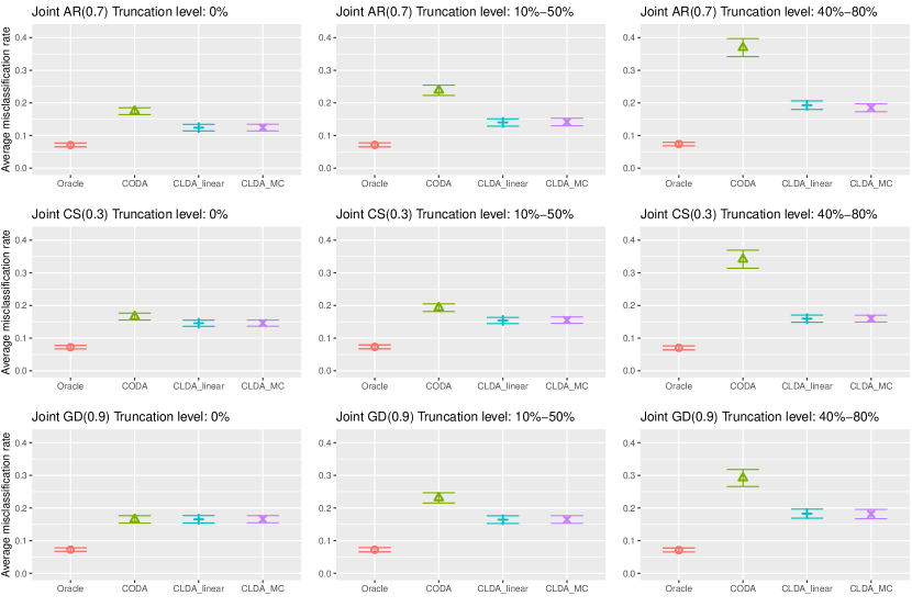
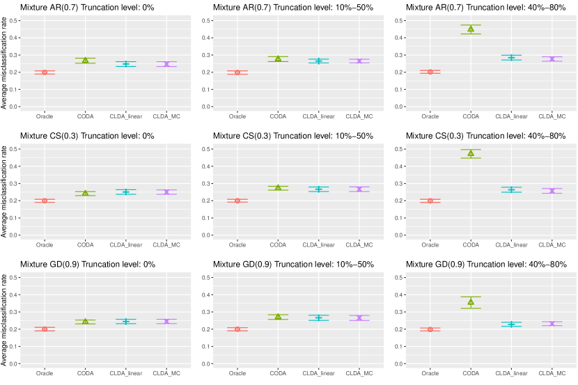
Figure 2 displays the results for the mixture model in Section 4.2. While the mixture model favors CODA, the proposed CLDA performs as well as CODA when truncation levels are less than 50%: no truncation and low truncation settings. However, CODA shows a significant deterioration under the high truncation level, having average misclassification rates close to random guessing (0.5) under AR and CS covariance settings. This is not the case for proposed CLDA, which maintains excellent performance even when truncation levels are high. As in the joint model, the two approximations (9) and (10) of the conditional class probability, lead to similar misclassification rates across all truncation levels and covariance settings.
5 Application to Quantitative Microbiome Data
We consider the QMP data of Vandeputte et al. (2017), processed as in Yoon et al. (2019). The data contain genera from patients with Crohn’s disease , a type of inflammatory bowel disease, and healthy controls . Out of 101 genera, 39 have unknown names, and we label them as Unknown 1 – Unknown 39. The proportions of zeros across all 101 genera range from 1% to 96%, with 14 genera having no zeros. Our goal is to construct a classification rule that can separate patients with Crohn’s disease from the healthy controls, and identify genera that have the most influence on classification.
We compare the performance of CLDA_linear, CLDA_MC and CODA as in Section 4. We randomly split the data into 4/5 and 1/5 and use the former to train the classifiers via 5-fold cross-validation and the latter to evaluate their misclassification error rate. We choose the tuning parameters as described in Section 4.3 and use MC samples of size from (8) to compute the posterior probabilities (9) and (10). Table 1 displays the average misclassification rates and model sizes over 30 random splits. Overall, the proposed CLDA significantly outperforms CODA with lower misclassification rate and smaller model size. Specifically, CLDA has the average misclassification rate of less than 3%, whereas CODA’s rate is around 9%. Futhermore, CLDA uses fewer genera for classification, selecting 14 variables on average, which is about 1/3 of the average model size of CODA, 37. The associated standard error of CLDA is also significantly smaller, indicating a more stable variable selection. The two approximations of the posterior probability used by CLDA, (9) and (10), lead to nearly identical misclassification rates, model sizes, and standard errors.
| Misclassification rate | Average model size | |
|---|---|---|
| CLDA_linear | 0.028 (0.005) | 13.4 (0.8) |
| CLDA_MC | 0.027 (0.006) | 13.7 (1.0) |
| CODA | 0.092 (0.011) | 36.8 (2.8) |
We further investigate and compare the selected genera by CLDA and CODA by considering their selection probabilities across 30 random splits. Table 2 lists the genera that are selected more than 90% of the times, i.e., at least 27 times out of 30. As before, there is agreement between the results of CLDA_linear and CLDA_MC. Both CLDA and CODA consistently select Fusobacterium. We find that the CLDA-estimated coefficients of Fusobacterium in are negative across all random splits indicating that an increase in Fusobacterium is positively associated with Crohn’s disease development (labelled as ). This result is consistent with existing findings (Han, 2015; Strauss et al., 2011) of positive correlation between Fusobacterium and inflammatory bowel disease. When looking beyond Fusobacterium, CLDA and CODA select non-overlapping genera. Observe that the remaining 12 genera with highest frequency for CODA all have no zeros or just a few zeros (less than 12%). In constrast, the remaining 2 genera for CLDA have a high proportion of zeros, with Succinivibrio (58.2% of zeros) selected 28 out of 30 times, and the unknown genera in the Comamonadaceae family (79.3% of zeros) selected 30 out of 30 times. We consider the CLDA-estimated coefficients of Succinivibrio, which are positive across all splits. This indicates that a subject with a high level of Succinivibrio is likely to be healthy. This finding is consistent with existing results from animal studies. Werner et al. (2011) argue that depletion of luminal iron can prevent Crohn’s disease, and subsequently find that mice feeding on an iron sulfate free diet show a significant increase of Succinivibrio. Given this biological evidence and the fact that CLDA has better misclassification error rate, we suspect that high zero inflation in Succinivibrio makes CODA miss this important variable, and that CODA has selection bias towards variables with smaller proportion of zeros as is seen in Table 2.
| Genera selected more than 27 times | ||
|---|---|---|
| CLDA_linear | CLDA_MC | CODA |
| Fusobacterium | Fusobacterium (48.9%) | Fusobacterium (48.9%) |
| Succinivibrio | Succinivibrio (58.2%) | Bacteroides (0%) |
| Unknown 8 | Unknown 8 (79.3%) | Bifidobacterium (2.2%) |
| Blautia (0%) | ||
| Coprococcus (0%) | ||
| Faecalibacterium (0%) | ||
| Prevotella (11.9%) | ||
| Roseburia (0%) | ||
| Ruminococcus (0%) | ||
| Unknown 11 (0%) | ||
| Unknown 25 (0%) | ||
| Unknown 35 (0%) | ||
| Unknown 5 (0%) | ||
6 Discussion
In this work we develop a binary classification model for zero-inflated data, and show the consistency of estimated classification direction in high-dimensional settings. On simulated data, our method achieves similar classification accuracy as existing competitor on continuous data, and significantly better accuracy on zero-inflated data. In an application to quantitative microbiome data, our method achieves significantly smaller misclassification error rate while also leading to a more parsimonious model. The selected genera align with existing results in microbiome literature.
There are several further research directions that could be pursued. First, our estimation consistency result is non-trivial leading us to develop a new technique to facilitate underlying theoretical analyses by combining sub-Gaussian properties of sign vector with newly established bounds on second derivatives of inverse bridge function for truncated/truncated cases. While this theoretical analysis has been restricted to mixed binary-truncated model in Definition 3, the developed technique can be applied more generally. In particular, it can be used to establish estimation consistency in high-dimensional settings within general semiparametric Gaussian copula regression modeling framework (Dey and Zipunnikov, 2022), which encompasses all continuous, binary, ordinal and truncated variable types. This generalization requires establishing bounds on first and second derivatives of corresponding inverse bridge functions, which while technical, can be accomplished in the similar ways as Section B.4 in Appendix. Secondly, our focus here is on binary classification problem, and multi-class extensions are of interest. In case the classes have a natural ordering, e.g., a disease classification as “Mild”, “Moderate” or “Severe”, the extension is straightforward by considering mixed ordinal-truncated model, with corresponding bridge function for ordinal/truncated case as derived in Huang et al. (2021). However, it is unclear how to incorporate unordered class labels due to ambiguity in the underlying latent Gaussian representation, making it a compelling question for future study.
Acknowledgements
The authors thank Grace Yoon for constructive discussions on QMP data analysis. This work has been partially supported by the Texas A&M Institute of Data Science (TAMIDS) and the Texas A&M Strategic Transformative Research Program. Gaynanova’s research was partially supported by the National Science Foundation (NSF CAREER DMS-2044823). Ni’s research was partially supported by the National Science Foundation (NSF DMS-1918851, NSF DMS-2112943). Portions of this research were conducted with the advanced computing resources provided by Texas A&M High Performance Research Computing.
Appendix A Appendix
A.1 First-order Taylor approximation of the posterior probability
Let and
Then, by Taylor,
A.2 Implementation details of CODA
CODA (Han et al., 2013) assumes that data satisfy the linear discriminant analysis assumption at the latent Gaussian level; that is,
| (16) |
where is the mean of class and is a common covariance matrix. To address the identifiability issue, CODA assumes that ’s preserves the population mean and variance, i.e.,
| (17) |
Under this model, the Bayes rule assigns a new observation to class 1 if
and class 0, otherwise, where and . The Bayes classification direction is estimated by solving
| (18) |
where , and are sample Kendall’s covariance matrices and . Given , the optimal intercept for a sparse LDA (Mai et al., 2012) is given by
Let , , be the sample class means and . The sample classification rule assigns a new observation to class 1 if
Appendix B Proofs of theoretical results
Throughout, we use to denote the bridge function such that for TT case with and . Here and are matrices of population and sample Kendall’s values, respectively, , with with , and with being the observed proportion of zeros in the th variable.
B.1 Proofs of theorems from the main manuscript
Definition 5 (Restricted eigenvalue condition).
A matrix satisfies restricted eigenvalue condition with parameter if for all sets with , and for all , it holds that
Theorem 4.
Under Assumption 4, if and satisfies RE(s,3) with parameter , then
Proof of Theorem 4.
This proof follows the proof of Theorem 2 in Gaynanova (2020). We repeat it here for completeness.
By the optimality condition of equation (9) in the main paper, we have
where is a subgradient of at . This gives
and thus
| (19) |
Since is a subgradient of at ,
| (20) |
By combining (19), (20), and Hölder’s and triangle inequalities, we have
Using condition on and Assumption 4,
Using the triangle inequality,
| (21) | ||||
| (22) | ||||
| (23) |
As is non-negative and , (22) implies that , and thus, is in the cone . Since satisfies RE() with paramter , we have
| (24) |
Using , (23) and (24) imply that
| (25) |
The bound for can be obtained as follows. Since ,
| (26) | ||||
| (27) | ||||
| (28) | ||||
| (29) | ||||
| (30) |
Let for notational simplicity. For , let be the index set of th largest (in absolute) components of . Then, as
Furthermore, it follows that for with last . Also, for , . Thus, by the triangle inequality,
| (31) | ||||
| (32) |
Using that satisfies RE and ,
∎
Proof.
Using and triangle inequality, we have
For , it follows from Theorem 7 of Yoon et al. (2020) that, for some ,
| (33) |
with probability at least .
Consider . Recall that , and , and let be the partial derivative of the inverse bridge function with respect to . By adding and subtracting from and applying the mean value theorem to with respect to ,
where and . Therefore
By letting
we further have, by the triangle inequality, that
We separately bound , , and in Lemmas 1, 2, and 3, respectively. Combining these bounds with (33) completes the proof. ∎
Proof.
B.2 Main supporting lemmas
Proof.
Let be the vector with 1 in the th component and 0 otherwise. Then, we have
where and is a deterministic unit vector. Since for some constant by Theorem 6 of Yoon et al. (2020), we have by Lemma 4. Therefore,
Consider . By Lemma 8, for any and ,
Letting and , we have
Thus, for some constant , with probability at least . ∎
Proof.
By the mean value theorem, for some , where , we have
where is the 2nd partial derivative of inverse bridge function with respect to . By Lemma 11, for some constant . Since , by Hölder’s inequality,
By Lemma 9, with probability at least , and by Lemma 4, . Thus, under Assumption 5, for sufficiently large and some constant ,
with probability at least . ∎
Proof.
We reparameterize and write , where . We also write and . For each element of , the multivariate mean value theorem gives
for some and , respectively.
Consider . By adding and subtracting to , we have that
By applying the multivariate mean value theorem to , we further have that
for some , , and . Thus, by the triangle inequality,
| (34) | ||||
| (35) | ||||
| (36) | ||||
| (37) |
where and . We consider (34)–(36) and (37) separately as follows.
For (34)–(36), we know that , , and are bounded above by some positive constants by Lemmas 14, 12, 13, respectively. Also, for some constant , and with probability at least by Lemmas 5 and 9. Since , and
Hence, we can show that, for some constant , (34)–(36) are bounded above by with probability at least by following the steps of Lemma 1.
For (37), we know that is bounded above by some positive constant by Lemma 10. Thus, by following the steps of Lemma 2, we can show that, for some constant , (37) is bounded above by with probability at least . By combining these results, we have that, for some constant ,
| (38) |
with probability at least .
By symmetrically applying above steps to , we also have that, for some constant ,
| (39) |
with probability at least . Combining (38) and (39) completes the proof.
∎
Proof.
Lemma 5.
For , let and , where . Also, let and . Then for any deterministic and ,
for some constant .
Proof.
For , let such that . By definition of the truncated latent Gaussian copula model, we have
Since , where and , is -subgaussian by Lemma 7, and thus is sum of iid -subgaussians. Thus,
∎
Lemma 6.
Proof.
Let . Let be the index set of the largest elements of in absolute value. Then it holds that , and
| (40) |
Furthermore, following (32), it holds that
| (41) |
Consider
| (42) |
Following the proof of Theorem 5 and reparameterization of in terms of , we have the following decomposition
| (43) |
where , , , and . We will use one technique to bound all first order terms in (43), and another technique to bound all second-order terms.
Consider second-order terms in (43). Each term is bounded in the same way using Hölder’s inequality and bounds on second derivatives. Concretely, consider the term corresponding to , that is
By Lemma 11, the 2nd derivative is bounded , thus, since is between and ,
Using the bound (40) on , the condition that satisfies RE, and Lemma 9, it follows that with high probability
All the remaining 2nd order terms have the same bound as all the second derivatives are bounded, that is by Lemma 12, by Lemma 14, by Lemma 13. Also with high probability by Hoeffding’s inequality combined with union bound, and with high probability by Lemma 9.
Consider first-order terms in (43). Each term is bounded in the same way using sub-gaussian properties in Lemma 5 (for ) and Lemma 8 (for ) combined with the fact that the first derivatives are both bounded and fixed. Concretely, consider the term corresponding to , that is
where and the last inequality follow from (40). From Theorem 6 of Yoon et al. (2020), for some constant , hence using (41)
Combining this bound with Lemma 9, and following the proof of Lemma 1 gives, with high probability,
and using that satisfies RE gives
All the remaining first order terms have the same bound as the first derivatives are fixed and bounded by Lemma 10, and satisfy Lemma 5.
Combining the bounds on the first and second-order terms coupled with Assumption 5 gives with high probability
Combining this bound with (42) gives
Under the scaling of Assumption 5, , thus it follows that for some constant .
∎
B.3 Supporting lemmas based on existing results
Lemma 7 (Barber and Kolar (2018) Lemma 4.5).
Let . Then is -subgaussian.
Lemma 8 (Barber and Kolar (2018) Lemma E.2).
For fixed and with , for any ,
Lemma 9 (De la Pena and Giné (2012) Theorem 4.1.8).
For any ,
with probability at least . With , with probability at least .
B.4 Bounds on partial derivatives of the inverse bridge function
Lemma 10.
Proof.
Lemma 11.
Proof.
Lemma 12.
Proof.
Lemma 13.
Proof.
Lemma 14.
B.5 Bounds on the partial derivatives of the bridge function
Here we bound partial derivatives of the bridge function for TT case, where
As the bridge function consists of two 4-dimensional Gaussian distribution functions, we will show that, whether or , the absolute values of partial derivatives of are bounded from above.
Proof.
By the Leibniz rule,
Thus, regardless of or ,
where is the conditional pdf given . Therefore, the three-dimensional integral above corresponds to a probability (and is bounded by one), leading to
The proof for is analogous. ∎
Proof.
We start from the partial derivative with respect to given in Lemma 15 as
Let and consider the following multivariate chain rule:
In the above, we only consider partial derivatives with respect to , , , and because , do not involve whether or , i.e., .
Consider the case . By Plackett (1954),
where is the conditional pdf given , , and . Therefore, above integral corresponds to a probability (and is bounded by one), leading to
where above inequalities hold because and . As Lemma 20 provides that for some constant , we have the desired result. The case is similar with the same bound.
For , again by Plackett (1954), we have
For notational convenience, let and write
| (45) |
where is the th row of . Then, by extending the range of integrations, the absolute value of (45) is bounded above as
By the triangle inequality,
where the last inequality holds as . Under Assumption 2, ,. By Lemma 20, whether or , is bounded above and all elements of are all bounded above. Thus, we have
By Lemma 23, for some constant ,
This concludes the proof and the proof for is analogous.
∎
Proof.
Proof.
By the Leibniz rule,
where is the conditional pdf given and . Thus, the two-dimensional integral above corresponds to a probability (and is bounded by one), leading to
where . As Lemma 20 provides that for some constant , this concludes the proof. ∎
Proof.
We start from the partial derivative with respect to given in Theorem 6 of Yoon et al. (2020) as
where is defined as
and the rest of ’s are analogously defined.
As is a sum of ’s, we show that is bounded above for all and whether and . Using the multivariate chain rule and triangle inequality,
By Lemma 26, for all and , for some constant . Also, as ’s are linear in , ’s are bounded above some positive constant. This concludes the proof. ∎
B.6 Auxillary lemmas
From Theorem 4 in Yoon et al. (2020), the bridge function for TT case takes the following form
with , ,
| (49) |
Lemma 20.
Let or from above, and let its inverse be . Under Assumption 1, , , for some constant . Also, for some constant regardless of or .
Proof.
Lemma 21.
Proof.
Since and is a decreasing function,
Furthermore, as the second derivative is given by
we have
∎
Lemma 22.
Let . Then, it follows that regardless of or , the conditional distribution of given is , where
Proof.
The results follow from the properties of conditional normal distribution using the form of and . ∎
Proof.
We first calculate the conditional means and covariance matrices using the properties of multivariate Gaussian distribution to obtain:
and
Consider . From the above, it is clear that all conditional variances are bounded below by some positive constant. It can be also seen that all conditional variances are bounded above as long as for some constant . Under Assumptions 1, and thus .
Consider . If or , then and the result is immediate under Assumption 2. For , let and , where detailed expressions are given above. Then, by Lemma 27, we have that
We can see from the above conditional means that, under Assumptions 1 and 2, is bounded above by some positive constant. As we already showed that is bounded above, the proof is complete. ∎
Lemma 24.
Proof.
It follows by the conditional mean and variance formulas of the multivariate Gaussian distribution that, regardless of or ,
and
Under Assumptions 1 and 2, the absolute values of the conditional means and conditional variances are bounded above by and , respectively. Then the result follows by Lemma 27. ∎
Lemma 25.
Let , where or . Then, for any and ,
for some constant .
Proof.
Let and write . We prove this lemma by considering the following three cases: , namely cases 1, 2, and 3, respectively.
Case 1.
Case 2.
Case 3.
Lemma 26.
Let , where . Then, for any and ,
for some constant .
Proof.
Let , . We write and , where.
We consider three cases where .
Consider the case , i.e., . For notational convenience, we write and . Then,
where the last equality is due to Plackett (1954). Let be the th row of , , and . By differentiating the multivariate Gaussian density, we have
We also have that for any , and by Lemma 20, for some constant . Thus,
The absolute value of the integral of the last term is bounded as
where the second inequality is due to expanding the range of integration, and the third inequality is due to the triangle inequality. By Lemma 20, we know that, whether or , , for all . Also, by the triangle inequality,
Hence, for some constant ,
where the last inequality holds by Lemma 25.
Consider the case . We assume, without loss of generality, that and , i.e., . Then, by Plackett (1954),
For notational convenience, let and write
Then, we have that
where the last inequality holds by the triangle inequality. By Lemma 20, for all , and by Assumption 2, for all for . This gives
Again, by Lemma 20, , and by Lemma 24, above integral is bounded above by some positive constant. Thus,
for some constant . ∎
Lemma 27.
Let . Then
Proof.
For , follows the followed Gaussian distribution with mean
Since and , , we have that
∎
References
- Ahn et al. (2021) Ahn, J., H. C. Chung, and Y. Jeon (2021). Trace ratio optimization for high-dimensional multi-class discrimination. Journal of Computational and Graphical Statistics 30(1), 192–203.
- Ahn and Marron (2010) Ahn, J. and J. Marron (2010). The maximal data piling direction for discrimination. Biometrika 97(1), 254–259.
- Barber and Kolar (2018) Barber, R. F. and M. Kolar (2018). Rocket: Robust confidence intervals via kendall’s tau for transelliptical graphical models. The Annals of Statistics 46(6B), 3422–3450.
- Bickel and Levina (2004) Bickel, P. J. and E. Levina (2004). Some theory for fisher’s linear discriminant function,naive bayes’, and some alternatives when there are many more variables than observations. Bernoulli 10(6), 989–1010.
- Bickel et al. (2009) Bickel, P. J., Y. Ritov, and A. B. Tsybakov (2009). Simultaneous analysis of lasso and dantzig selector. The Annals of statistics 37(4), 1705–1732.
- Chikuse (2003) Chikuse, Y. (2003). Statistics on Special Manifolds, Volume 174. Springer New York, NY.
- Clemmensen et al. (2011) Clemmensen, L., T. Hastie, D. Witten, and B. Ersbøll (2011). Sparse discriminant analysis. Technometrics 53(4), 406–413.
- De la Pena and Giné (2012) De la Pena, V. and E. Giné (2012). Decoupling: from dependence to independence. Springer Science & Business Media.
- Dey and Zipunnikov (2022) Dey, D. and V. Zipunnikov (2022). Semiparametric gaussian copula regression modeling for mixed data types (sgcrm). arXiv preprint arXiv:2205.06868.
- Dong et al. (2016) Dong, K., H. Zhao, T. Tong, and X. Wan (2016). Nblda: negative binomial linear discriminant analysis for rna-seq data. BMC bioinformatics 17(1), 1–10.
- Fan et al. (2017) Fan, J., H. Liu, Y. Ning, and H. Zou (2017). High dimensional semiparametric latent graphical model for mixed data. Journal of the Royal Statistical Society: Series B (Statistical Methodology) 79(2), 405–421.
- Feng and Ning (2019) Feng, H. and Y. Ning (2019). High-dimensional Mixed Graphical Model with Ordinal Data - Parameter Estimation and Statistical Inference. AISTATS.
- Gaynanova (2020) Gaynanova, I. (2020). Prediction and estimation consistency of sparse multi-class penalized optimal scoring. Bernoulli 26(1), 286–322.
- Gaynanova (2021) Gaynanova, I. (2021). MGSDA: Multi-Group Sparse Discriminant Analysis. R package version 1.6.
- Gaynanova et al. (2016) Gaynanova, I., J. G. Booth, and M. T. Wells (2016). Simultaneous sparse estimation of canonical vectors in the p N setting. Journal of the American Statistical Association 111(514), 696–706.
- Guo et al. (2007) Guo, Y., T. Hastie, and R. Tibshirani (2007). Regularized linear discriminant analysis and its application in microarrays. Biostatistics 8(1), 86–100.
- Han and Liu (2014) Han, F. and H. Liu (2014). Scale-invariant sparse PCA on high-dimensional meta-elliptical data. Journal of the American Statistical Association 109(505), 275–287.
- Han et al. (2013) Han, F., T. Zhao, and H. Liu (2013). CODA: High dimensional copula discriminant analysis. Journal of Machine Learning Research 14, 629–671.
- Han (2015) Han, Y. W. (2015). Fusobacterium nucleatum: a commensal-turned pathogen. Current Opinion in Microbiology 23, 141–147.
- Hastie et al. (2009) Hastie, T., R. Tibshirani, J. H. Friedman, and J. H. Friedman (2009). The elements of statistical learning: data mining, inference, and prediction, Volume 2. Springer New York, NY.
- (21) Hastie, T., R. Tibshirani, and M. Wainwright. Statistical Learning with Sparsity. The Lasso and Generalizations. CRC Press.
- Hernández and Velilla (2005) Hernández, A. and S. Velilla (2005). Dimension reduction in nonparametric kernel discriminant analysis. Journal of Computational and Graphical Statistics 14(4), 847–866.
- Huang et al. (2021) Huang, M., C. L. Müller, and I. Gaynanova (2021). latentcor: An r package for estimating latent correlations from mixed data types. Journal of Open Source Software 6(65), 3634.
- Lapanowski and Gaynanova (2019) Lapanowski, A. F. and I. Gaynanova (2019). Sparse feature selection in kernel discriminant analysis via optimal scoring. In The 22nd International Conference on Artificial Intelligence and Statistics, pp. 1704–1713. PMLR.
- Lee et al. (2013) Lee, M. H., J. Ahn, and Y. Jeon (2013). Hdlss discrimination with adaptive data piling. Journal of Computational and Graphical Statistics 22(2), 433–451.
- Lin and Jeon (2003) Lin, Y. and Y. Jeon (2003). Discriminant analysis through a semiparametric model. Biometrika 90(2), 379–392.
- Liu et al. (2009) Liu, H., J. D. Lafferty, and L. Wasserman (2009). The Nonparanormal: Semiparametric Estimation of High Dimensional Undirected Graphs. Journal of Machine Learning Research 10, 2295–2328.
- Mai et al. (2012) Mai, Q., H. Zou, and M. Yuan (2012). A direct approach to sparse discriminant analysis in ultra-high dimensions. Biometrika 99(1), 29–42.
- Negahban et al. (2012) Negahban, S. N., P. Ravikumar, M. J. Wainwright, and B. Yu (2012). A unified framework for high-dimensional analysis of -estimators with decomposable regularizers. Statistical science 27(4), 538–557.
- Plackett (1954) Plackett, R. L. (1954). A reduction formula for normal multivariate integrals. Biometrika 41(3-4), 351–360.
- Quan et al. (2018) Quan, X., J. G. Booth, and M. T. Wells (2018). Rank-based approach for estimating correlations in mixed ordinal data. arXiv.org.
- Silverman et al. (2020) Silverman, J. D., K. Roche, S. Mukherjee, and L. A. David (2020). Naught all zeros in sequence count data are the same. Computational and structural biotechnology journal 18, 2789–2798.
- Strauss et al. (2011) Strauss, J., G. G. Kaplan, P. L. Beck, K. Rioux, R. Panaccione, R. DeVinney, T. Lynch, and E. Allen-Vercoe (2011). Invasive potential of gut mucosa-derived fusobacterium nucleatum positively correlates with IBD status of the host. Inflammatory Bowel Diseases 17(9), 1971–1978.
- Vandeputte et al. (2017) Vandeputte, D., G. Kathagen, K. D’hoe, S. Vieira-Silva, M. Valles-Colomer, J. Sabino, J. Wang, R. Y. Tito, L. De Commer, Y. Darzi, et al. (2017). Quantitative microbiome profiling links gut community variation to microbial load. Nature 551(7681), 507–511.
- Werner et al. (2011) Werner, T., S. J. Wagner, I. Martinez, J. Walter, J.-S. Chang, T. Clavel, S. Kisling, K. Schuemann, and D. Haller (2011). Depletion of luminal iron alters the gut microbiota and prevents crohn’s disease-like ileitis. Gut 60(3), 325–333.
- Witten (2011) Witten, D. M. (2011). Classification and clustering of sequencing data using a Poisson model. The Annals of Applied Statistics 5(4), 2493–2518.
- Witten and Tibshirani (2011) Witten, D. M. and R. Tibshirani (2011). Penalized classification using Fisher’s linear discriminant. Journal of the Royal Statistical Society: Series B (Statistical Methodology) 73(5), 753–772.
- Yoon et al. (2020) Yoon, G., R. J. Carroll, and I. Gaynanova (2020). Sparse semiparametric canonical correlation analysis for data of mixed types. Biometrika 107(3), 609–625.
- Yoon and Gaynanova (2021) Yoon, G. and I. Gaynanova (2021). Sparse Canonical Correlation Analysis for High-Dimensional Mixed Data. R package version 1.4.6.
- Yoon et al. (2019) Yoon, G., I. Gaynanova, and C. L. Müller (2019). Microbial networks in spring-semi-parametric rank-based correlation and partial correlation estimation for quantitative microbiome data. Frontiers in Genetics 10, 516.