1 Introduction

The $\mathcal{Z}_{2}\times\mathcal{Z}_{N}$ flavour symmetry[1] provides a new framework for the celebrated Froggatt-Nielsen (FN) mechanism that eventually furnishes an elegant solution to the flavour problem of the standard model (SM)[2]. The flavour problem of the SM comprises a set of fundamental questions, including the origin of the mass pattern of fermions of the SM, an explanation for the observed quark-mixing, and the source of neutrino masses and oscillations. There are various approaches to address this problem in literature. For instance, it can have a solution through the hierarchy of vacuum-expectation-values (VEVs) in a technicolour-framework where VEVs are sequential chiral condensates of an extended dark-technicolour sector[3, 4, 5]. A possible explanation can be obtained using Abelian flavor symmetries [2, 6, 7, 8, 9, 10], creating loop-suppressed couplings to the Higgs [11], through wave-function localization [12] or via compositeness [13].

The central idea of the FN mechanism mechanism is based on an Abelian flavour symmetry $U(1)_{F}$, which can distinguish different flavours of fermions among and within the fermionic generations in the SM. This is achieved by introducing a flavon field $\chi$ in such a way that only top quark gets mass from a renormalized SM interaction, and masses for other fermions are obtained from appropriate non-renormalized higher dimensional operators, which are constructed using the flavon field $\chi$. For instance, if under the $U(1)_{F}$ symmetry the fermions $\psi_{i}^{c}$ and $\psi_{j}$ have charges $\theta_{i}$ and $\theta_{j}$ respectively and the charge of the the SM Higgs field is zero then the Yukawa Lagrangian of the SM is forbidden by the $U(1)_{F}$ symmetry. In this scenario, the masses of the SM fermions can be recovered by the non-renormalizable operators of the form,

$$\mathcal{O} = y(\dfrac{\chi}{\Lambda})^{(\theta_{i}+\theta_{j})}\bar{\psi}\varphi\psi,$$

$$= y\epsilon^{(\theta_{i}+\theta_{j})}\bar{\psi}\varphi\psi=Y\bar{\psi}\varphi\psi$$

where $y$ is the dimensionless coupling constant, $\Lambda$ is the scale at which these operators are renormalized, $\epsilon=\dfrac{\langle\chi\rangle}{\Lambda}$, $Y=y\epsilon^{(\theta_{i}+\theta_{j})}$ is the effective Yukawa coupling, and the gauge singlet flavon scalar field $\chi$ transforms under the $SU(3)_{c}\times SU(2)_{L}\times U(1)_{Y}$ symmetry of the SM as,

$$\chi:(1,1,0).$$ (2)

The $U(1)_{F}$ flavour symmetry is broken spontaneously when the flavon field $\chi$ acquires a VEV. The scale $\Lambda$ is not provided by the theory, and it can be anywhere between the weak and the Planck scale. We only require that the flavour symmetry should be broken weakly which means the ratio $\dfrac{\langle\chi\rangle}{\Lambda}$ should be less than unity. The flavon exchange effects in the SM phenomenology will be highly suppressed if the scale of new physics $\Lambda$ is much larger than the weak scale. However, if the flavour symmetry is broken close to the weak scale, we can hope to see observable effects on the direct or indirect experimentally measured SM observables such as mixing and $CP$-violation in mesons. Therefore, we need to ask how low the flavour scale could be such that it respects the bounds on flavour-changing and CP-violating processes. Moreover, the nature of the flavour symmetry also plays an important role in the investigation of the flavour scale. For example, if the flavour symmetry is a continuous $U(1)_{F}$, then we should ask whether it is a gauged or a global symmetry. In a gauged $U(1)_{F}$ scenario, the phenomenology of the flavon field will be affected by the exchange of the corresponding gauge boson. If the continuous $U(1)_{F}$ is global, then a massless Goldstone boson must exist.

The $\mathcal{Z}_{2}\times\mathcal{Z}_{N}$ flavour symmetry, unlike the conventional continuous $U(1)$ flavour symmetry that is employed to achieve the FN mechanism, is a product of two discrete symmetries which can implement the FN mechanism in a unique way such that the flavour structure of the SM including neutrino masses and mixing parameters can be parametrized in terms of a small parameter which is the ratio of the VEV of the flavon field and the flavour scale $\Lambda$[1]. We notice that the origin of the $\mathcal{Z}_{2}\times\mathcal{Z}_{N}$ flavour symmetry may be traced to an underlying Abelian or non-Abelian continuous symmetry or their products. For instance, the $\mathcal{Z}_{2}\times\mathcal{Z}_{N}$ symmetry may be a by-product of a spontaneous breaking of $U(1)\times U(1)$ continuous product symmetry.

We note that the discrete $\mathcal{Z}_{2}$ symmetry is extensively used in studying the different versions of the two-Higgs-doublet model (2HDM) and the minimal supersymmetric SM (MSSM). In particular, in the $\mathcal{Z}_{2}\times\mathcal{Z}_{N}$ flavour symmetry, the discrete $\mathcal{Z}_{2}$ symmetry exactly behaves like the one used in the type-ii@ 2HDM[14]. Therefore, the $\mathcal{Z}_{2}\times\mathcal{Z}_{N}$ flavour symmetry may also be used to implement the FN mechanism in the type-ii@ 2HDM and the MSSM. Moreover, the discrete $\mathcal{Z}_{2}$ symmetry is also found to be useful in model building, for instance, see references [3, 5, 15, 16, 17, 18].

In this work, we investigate flavour bounds on the dynamics of the flavon field of a minimal and a non-minimal form of the $\mathcal{Z}_{2}\times\mathcal{Z}_{N}$ flavour symmetry that provides a simple set-up for the FN mechanism. We do not consider any ultraviolet completion of the $\mathcal{Z}_{2}\times\mathcal{Z}_{N}$ based FN mechanism, and present our results in a model-independent manner. The phenomenological investigations of the flavon field of the FN mechanism in the framework of a continuous $U(1)$ symmetry and its extensions are dedicatedly performed in literature, for instance, flavour bounds are investigated in reference[19], the LHC phenomenology is explored in references[20, 21, 22, 23, 24, 25, 26, 27], a low flavour breaking scale is studied in reference [28], a study for a future high energy collider is presented in reference[29], flavon exchange effects in the dark matter interactions are studied in reference [30], the texture based investigation of the FN mechanism can be found in reference [31].

We shall present our phenomenological analysis along the following line: In section 2, we investigate a minimal form of the $\mathcal{Z}_{2}\times\mathcal{Z}_{N}$ flavour symmetry that can implement the FN mechanism. An explanation to neutrino masses and mixing parameters is discussed in section 2.4.1. A non-minimal form of the $\mathcal{Z}_{2}\times\mathcal{Z}_{N}$ flavour symmetry that implements the FN mechanism is discussed in section 3. The scalar potential of our model is discussed in section 4. Phenomenological bounds based on the quark flavour physics on the parameter space of a minimal and a non-minimal form of the $\mathcal{Z}_{2}\times\mathcal{Z}_{N}$ flavour symmetry are derived in section 5. Leptonic flavour constraints are investigated in section 6. A summary of the work is presented in section 7.

2 A minimal $\mathcal{Z}_{2}\times\mathcal{Z}_{N}$ flavour symmetry

We now discuss the question of a minimal form of the $\mathcal{Z}_{2}\times\mathcal{Z}_{N}$ flavour symmetry that can provide a simple set-up of the FN mechanism. Our guiding principle for this purpose is the observation that a minimal suppression of the effective Yukawa couplings will require a minimal form of the $\mathcal{Z}_{2}\times\mathcal{Z}_{N}$ flavour symmetry. For instance, we assume that the mass of the top quark originates from the tree level SM Yukawa operator, then, following the principle of minimum suppression (PMS), the mass of the bottom quark is obtained from the operator having the suppression of the order $y\epsilon$, the mass of the charm quark from the operator having the suppression of the order $y\epsilon^{2}$, the mass of the strange quark from the operator having the suppression of the order $y\epsilon^{3}$, and the mass of the up and down quarks from the operators having at least the suppression of the order $y\epsilon^{4}$.

Additionally, we need to count the number of hierarchical energy scales needed to account for the fermionic mass hierarchy in the SM. For instance, for the quark sector, we need three energy scales to explain the mass hierarchy among the three fermionic families. We note that only the second and the third quark families have intra-generational mass hierarchies, which require only two hierarchical energy scales to achieve an explanation for the mass hierarchy within the second and third quark families. These hierarchical energy scales are created by the different non-renormalizable operators of the flavon fields as given in equation 1. Since the mass of the top quark is generated by the renormalized SM Yuakwa operators, at least four energy scales are required to be created through the operators of the form given in equation 1 for providing an explanation for the hierarchical quark mass pattern.

The symmetry $\mathcal{Z}_{N}$ in the $\mathcal{Z}_{2}\times\mathcal{Z}_{N}$ flavour symmetry is responsible for providing such operators. The symmetry $\mathcal{Z}_{2}$ distinguishes between the up-type and the down-type quarks, which makes sure that identical non-renormalizable operators of the flavon fields, as given in equation 1, do not appear in the up and down-type quark mass matrices. For creating four energy scales, the required $\mathcal{Z}_{N}$ symmetry, therefore, should have at least four non-trivial charges. Therefore, the size of a minimal symmetry will be determined by this requirement and through the application of the PMS.

Finally, we must note that a minimal form of the $\mathcal{Z}_{2}\times\mathcal{Z}_{N}$ flavour symmetry should not only produce correct pattern of the charged fermion masses, it should be capable of explaining the quark mixing pattern, neutrino masses, and more importantly, it should predict correct pattern of the neutrino mixing angles.

After taking into account above considerations, $\mathcal{Z}_{2}\times\mathcal{Z}_{N}$ flavour symmetry allows us to write the following generic Lagrangian which provides masses to the charged fermions of the SM,

$$-{\mathcal{L}}_{\rm Yukawa} = \left[\dfrac{\chi(\chi^{\dagger})}{\Lambda}\right]^{n_{ij}^{u}}y_{ij}^{u}\bar{\psi}_{L_{i}}^{q}\tilde{\varphi}\psi_{R_{j}}^{u}+\left[\dfrac{\chi(\chi^{\dagger})}{\Lambda}\right]^{n_{ij}^{d}}y_{ij}^{d}\bar{\psi}_{L_{i}}^{q}\varphi\psi_{R_{j}}^{d}$$

$$+ \left[\dfrac{\chi(\chi^{\dagger})}{\Lambda}\right]^{n_{ij}^{\ell}}y_{ij}^{\ell}\bar{\psi}_{L_{i}}^{\ell}\varphi\psi_{R_{j}}^{\ell}+{\rm H.c.},$$

$$= Y^{u}_{ij}\bar{\psi}_{L_{i}}^{q}\tilde{\varphi}\psi_{R_{j}}^{u}+Y^{d}_{ij}\bar{\psi}_{L_{i}}^{q}\varphi\psi_{R_{j}}^{d}+Y^{\ell}_{ij}\bar{\psi}_{L_{i}}^{\ell}\varphi\psi_{R_{j}}^{\ell}+\text{H.c.},$$

where $\chi$ or $\chi^{\dagger}$ may appear in the numerator of the term inside the square brackets. We note that in the above Lagrangian $i$ and $j$ are family indices, $\psi_{L}^{q},\psi_{L}^{\ell}$ are quark and leptonic doublets, $\psi_{R}^{u},\psi_{R}^{d},\psi_{R}^{\ell}$ are right-handed up, down type singlet quarks and leptons, $\varphi$ and $\tilde{\varphi}=-i\sigma_{2}\varphi^{*}$ are the SM Higgs field and its conjugate and $\sigma_{2}$ is the second Pauli matrix. The effective Yukawa couplings $Y_{ij}$ are defined in terms of the expansion parameter $\dfrac{\langle\chi\rangle}{\Lambda}=\dfrac{f}{\sqrt{2}\Lambda}=\epsilon<<1$ such that $Y_{ij}=y_{ij}\epsilon^{n_{ij}}$.

2.1 $\mathcal{Z}_{2}\times\mathcal{Z}_{2}$ flavour symmetry

The simplest choice is the $\mathcal{Z}_{2}\times\mathcal{Z}_{2}$ flavour symmetry, which turns out to be a trivial selection since the only charges of the $\mathcal{Z}_{2}$ symmetry are $\pm 1$, which are too trivial to provide four energy scales or equivalently non-trivial operators of the form given in equation 1. Hence, we conclude that this symmetry cannot be used to create a simple FN mechanism.

2.2 $\mathcal{Z}_{2}\times\mathcal{Z}_{3}$ flavour symmetry

The first non-trivial form of the $\mathcal{Z}_{2}\times\mathcal{Z}_{N}$ flavour symmetry, which may provide an implementation of the FN mechanism, is $\mathcal{Z}_{2}\times\mathcal{Z}_{3}$. The symmetry $\mathcal{Z}_{3}$ has two non-trivial charges characterized by $\omega$ and $\omega^{2}$, where $\omega$ is the cube root of unity. In the first scenario, following the PMS, we assign the charges to the SM and flavon fields as given in table 1.

Fields	$\mathcal{Z}_{2}$	$\mathcal{Z}_{3}$
$u_{R},c_{R},t_{R}$	+	$\omega$
$d_{R},s_{R},b_{R},e_{R},\mu_{R},\tau_{R}$	-	$1$
$\psi_{L_{1}}^{q}$	+	$\omega^{2}$
$\psi_{L_{2}}^{q}$	+	$1$
$\psi_{L_{3}}^{q}$	+	$\omega$
$\psi_{L_{1}}^{\ell}$	+	$\omega^{2}$
$\psi_{L_{2}}^{\ell}$	+	$1$
$\psi_{L_{3}}^{\ell}$	+	$\omega$
$\chi$	-	$\omega$
$\varphi$	+	1

Table 1: The charges of left and right-handed fermions of three families of the SM, Higgs and the flavon field under the $\mathcal{Z}_{2}$ and $\mathcal{Z}_{3}$ product symmetry, where $\omega$ is the cube root of unity.

We observe that the masses of $s$ and $b$ quarks can be recovered from this charge assignment, for instance, mass of the $s$ quark is of the order $\epsilon^{3}$, and that of the $b$ quark is of the order $\epsilon$. However, the mass of the $u$ and $d$ quarks are produced by the operators $y(\dfrac{\chi^{\dagger}}{\Lambda})^{2}\bar{\psi}\varphi u_{R}$ and $y(\dfrac{\chi^{\dagger}}{\Lambda})\bar{\psi}\varphi d_{R}$ instead of the operators $y(\dfrac{\chi}{\Lambda})^{4}\bar{\psi}\varphi u_{R}$ and $y(\dfrac{\chi}{\Lambda})^{5}\bar{\psi}\varphi d_{R}$. Any other charge assignment also does not reproduce masses of every quark.

As an additional check, we may assume that exactly identical diagonal operators for the $u$ and $d$ quarks in their mass matrices as given in table 2. This charge assignment is against the original sprite of the $\mathcal{Z}_{2}\times\mathcal{Z}_{N}$ flavour symmetry, where the $\mathcal{Z}_{2}$ is exactly like the symmetry used in the type ii@ 2HDM. It turns out that even in this case, the mass of the $u$ quark is of the order $\epsilon$. This conclusion does not change even if we provide different non-trivial charge assignments to the fermions and flavon fields under the $\mathcal{Z}_{2}\times\mathcal{Z}_{3}$ flavour symmetry.

Fields	$\mathcal{Z}_{2}$	$\mathcal{Z}_{3}$
$c_{R},t_{R}$	+	$\omega$
$u_{R},d_{R},s_{R},b_{R},e_{R},\mu_{R},\tau_{R}$	-	$1$
$\psi_{L_{1}}^{q}$	+	$\omega^{2}$
$\psi_{L_{2}}^{q}$	+	$1$
$\psi_{L_{3}}^{q}$	+	$\omega$
$\psi_{L_{1}}^{\ell}$	+	$\omega^{2}$
$\psi_{L_{2}}^{\ell}$	+	$1$
$\psi_{L_{3}}^{\ell}$	+	$\omega$
$\chi$	-	$\omega$
$\varphi$	+	1

Table 2: The charges of left and right-handed fermions of three families of the SM, Higgs and the flavon fields under the $\mathcal{Z}_{2}$ and $\mathcal{Z}_{3}$ product symmetry, where $\omega$ is the cube root of unity.

2.3 $\mathcal{Z}_{2}\times\mathcal{Z}_{4}$ flavour symmetry

The charges of the symmetry $\mathcal{Z}_{2}\times\mathcal{Z}_{4}$ are characterized by the fourth roots of unity, which are $1,\omega,\omega^{2}$ and $\omega^{3}$ where $\omega=i$, $\omega^{3}=\omega^{*}$ and $\omega^{2}=-1$. We particularly note that minimally suppressed diagonal operator of the form $y(\dfrac{\chi}{\Lambda})^{4}\bar{\psi}_{L}\varphi u_{R}$ is not the dominant operator no matter what charge we assign to the flavon and fermionic fields. This is because the tree-level SM Yukawa operator $y\bar{\psi}_{L}\varphi u_{R}$ is allowed for any charge assignment for the $y(\dfrac{\chi}{\Lambda})^{4}\bar{\psi}_{L}\varphi u_{R}$ operator under the $\mathcal{Z}_{2}\times\mathcal{Z}_{4}$ flavour symmetry.

Fields	$\mathcal{Z}_{2}$	$\mathcal{Z}_{4}$
$c_{R},t_{R}$	+	$\omega^{2}$
$u_{R},d_{R},s_{R},b_{R},e_{R},\mu_{R},\tau_{R}$	-	$\omega$
$\psi_{L_{1}}^{q}$	+	$\omega^{2}$
$\psi_{L_{2}}^{q}$	+	$1$
$\psi_{L_{3}}^{q}$	+	$\omega^{2}$
$\psi_{L_{1}}^{\ell}$	+	$\omega^{2}$
$\psi_{L_{2}}^{\ell}$	+	$1$
$\psi_{L_{3}}^{\ell}$	+	$\omega^{2}$
$\chi$	-	$\omega$
$\varphi$	+	1

Table 3: The charges of left and right-handed fermions of three families of the SM, Higgs and the flavon fields under the $\mathcal{Z}_{2}$ and $\mathcal{Z}_{4}$ product symmetry, where $\omega$ is the fourth root of unity.

Therefore, to produce the mass of the $u$-quark, we either choose a non-trivial transformation of the $u_{R}$-quark or the first family of the quarks under the $\mathcal{Z}_{2}$ symmetry, in addition to the next to the minimal suppressed operator of the order $\epsilon^{5}$. One such charge assignment is given in table 3. In this case, the masses of the down-type quarks are produced correctly through the operators with minimal suppression. However, in the case of up-type quarks, still non-diagonal tree-level SM operators dominate the mass of the $u$-quark. Other alternative charge assignments also do not work for creating an FN mechanism through the $\mathcal{Z}_{2}\times\mathcal{Z}_{4}$ symmetry.

2.4 $\mathcal{Z}_{2}\times\mathcal{Z}_{5}$ flavour symmetry

We now impose the next flavour symmetry, that is, the $\mathcal{Z}_{2}\times\mathcal{Z}_{5}$ symmetry on the SM in a way that the various fields of the SM transform under this symmetry as given in table 4[1]. As discussed earlier, we need to create at least four hierarchical energy scales as an origin of the quark mass spectrum. This means, for creating these energy scales, a non-trivial and a minimal $\mathcal{Z}_{N}$ symmetry should have at least four non-trivial charges. Thus, the symmetry $\mathcal{Z}_{5}$ could be such a symmetry. Moreover, we note that the transformation of fields under the $\mathcal{Z}_{2}\times\mathcal{Z}_{5}$ symmetry is chosen such that the symmetry $\mathcal{Z}_{2}$ exactly acts like the way used in the type-ii@ 2HDM .

Fields	$\mathcal{Z}_{2}$	$\mathcal{Z}_{5}$
$u_{R},c_{R},t_{R}$	+	$\omega^{2}$
$d_{R},s_{R},b_{R},e_{R},\mu_{R},\tau_{R}$	-	$\omega$
$\nu_{e_{R}},\nu_{\mu_{R}},\nu_{\tau_{R}}$	-	$\omega^{3}$
$\psi_{L_{1}}^{q}$	+	$\omega$
$\psi_{L_{2}}^{q}$	+	$\omega^{4}$
$\psi_{L_{3}}^{q}$	+	$\omega^{2}$
$\psi_{L_{1}}^{\ell}$	+	$\omega$
$\psi_{L_{2}}^{\ell}$	+	$\omega^{4}$
$\psi_{L_{3}}^{\ell}$	+	$\omega^{2}$
$\chi$	-	$\omega$
$\varphi$	+	1

Table 4: The charges of left and right-handed fermions of three families of the SM, right-handed neutrinos, Higgs, and singlet scalar fields under $\mathcal{Z}_{2}$ and $\mathcal{Z}_{5}$ symmetries, where $\omega$ is the fifth root of unity.

The $\mathcal{Z}_{2}\times\mathcal{Z}_{5}$ flavour symmetry allows us to write the following Lagrangian which provides masses to the charged fermions of the SM,

$$-{\mathcal{L}}_{\rm Yukawa} = \left(\dfrac{\chi}{\Lambda}\right)^{4}y_{11}^{u}\bar{\psi}_{L_{1}}^{q}\tilde{\varphi}u_{R}+\left(\dfrac{\chi}{\Lambda}\right)^{4}y_{12}^{u}\bar{\psi}_{L_{1}}^{q}\tilde{\varphi}c_{R}+\left(\dfrac{\chi}{\Lambda}\right)^{4}y_{13}^{u}\bar{\psi}_{L_{1}}^{q}\tilde{\varphi}t_{R}+\left(\dfrac{\chi}{\Lambda}\right)^{2}y_{21}^{u}\bar{\psi}_{L_{2}}^{q}\tilde{\varphi}u_{R}$$

$$+ \left(\dfrac{\chi}{\Lambda}\right)^{2}y_{22}^{u}\bar{\psi}_{L_{2}}^{q}\tilde{\varphi}c_{R}+\left(\dfrac{\chi}{\Lambda}\right)^{2}y_{23}^{u}\bar{\psi}_{L_{2}}^{q}\tilde{\varphi}t_{R}+y_{31}^{u}\bar{\psi}_{L_{3}}^{q}\tilde{\varphi}u_{R}+y_{32}^{u}\bar{\psi}_{L_{3}}^{q}\tilde{\varphi}c_{R}+y_{33}^{u}\bar{\psi}_{L_{3}}^{q}\tilde{\varphi}t_{R}$$

$$+ \left(\dfrac{\chi}{\Lambda}\right)^{5}y_{11}^{d}\bar{\psi}_{L_{1}}^{q}\varphi d_{R}+\left(\dfrac{\chi}{\Lambda}\right)^{5}y_{12}^{d}\bar{\psi}_{L_{1}}^{q}\varphi s_{R}+\left(\dfrac{\chi}{\Lambda}\right)^{5}y_{13}^{d}\bar{\psi}_{L_{1}}^{q}\varphi b_{R}+\left(\dfrac{\chi}{\Lambda}\right)^{3}y_{21}^{d}\bar{\psi}_{L_{2}}^{q}\varphi d_{R}$$

$$+ \left(\dfrac{\chi}{\Lambda}\right)^{3}y_{22}^{d}\bar{\psi}_{L_{2}}^{q}\varphi s_{R}+\left(\dfrac{\chi}{\Lambda}\right)^{3}y_{23}^{d}\bar{\psi}_{L_{2}}^{q}\varphi b_{R}+\left(\dfrac{\chi}{\Lambda}\right)y_{31}^{d}\bar{\psi}_{L_{3}}^{q}\varphi d_{R}+\left(\dfrac{\chi}{\Lambda}\right)y_{32}^{d}\bar{\psi}_{L_{3}}^{q}\varphi s_{R}$$

$$+ \left(\dfrac{\chi}{\Lambda}\right)y_{33}^{d}\bar{\psi}_{L_{3}}^{q}\varphi b_{R}+\left(\dfrac{\chi}{\Lambda}\right)^{5}y_{11}^{\ell}\bar{\psi}_{L_{1}}^{\ell}\varphi e_{R}+\left(\dfrac{\chi}{\Lambda}\right)^{5}y_{12}^{\ell}\bar{\psi}_{L_{1}}^{\ell}\varphi\mu_{R}+\left(\dfrac{\chi}{\Lambda}\right)^{5}y_{13}^{\ell}\bar{\psi}_{L_{1}}^{\ell}\varphi\tau_{R}$$

$$+ \left(\dfrac{\chi}{\Lambda}\right)^{3}y_{21}^{\ell}\bar{\psi}_{L_{2}}^{\ell}\varphi e_{R}+\left(\dfrac{\chi}{\Lambda}\right)^{3}y_{22}^{\ell}\bar{\psi}_{L_{2}}^{\ell}\varphi\mu_{R}+\left(\dfrac{\chi}{\Lambda}\right)^{3}y_{23}^{\ell}\bar{\psi}_{L_{2}}^{\ell}\varphi\tau_{R}+\left(\dfrac{\chi}{\Lambda}\right)y_{31}^{\ell}\bar{\psi}_{L_{3}}^{\ell}\varphi e_{R}$$

$$+ \left(\dfrac{\chi}{\Lambda}\right)y_{32}^{\ell}\bar{\psi}_{L_{3}}^{\ell}\varphi\mu_{R}+\left(\dfrac{\chi}{\Lambda}\right)y_{33}^{\ell}\bar{\psi}_{L_{3}}^{\ell}\varphi\tau_{R}+\text{H.c.}$$

The mass matrices for up- and down-type quarks and charged leptons can be written now in terms of the expansion parameter $\epsilon$,

$${\cal M}_{u}=\dfrac{v}{\sqrt{2}}\begin{pmatrix}y_{11}^{u}\epsilon^{4}&y_{12}^{u}\epsilon^{4}&y_{13}^{u}\epsilon^{4}\\ y_{21}^{u}\epsilon^{2}&y_{22}^{u}\epsilon^{2}&y_{23}^{u}\epsilon^{2}\\ y_{31}^{u}&y_{32}^{u}&y_{33}^{u}\end{pmatrix},{\cal M}_{d}=\dfrac{v}{\sqrt{2}}\begin{pmatrix}y_{11}^{d}\epsilon^{5}&y_{12}^{d}\epsilon^{5}&y_{13}^{d}\epsilon^{5}\\ y_{21}^{d}\epsilon^{3}&y_{22}^{d}\epsilon^{3}&y_{23}^{d}\epsilon^{3}\\ y_{31}^{d}\epsilon&y_{32}^{d}\epsilon&y_{33}^{d}\epsilon\end{pmatrix},{\cal M}_{\ell}=\dfrac{v}{\sqrt{2}}\begin{pmatrix}y_{11}^{\ell}\epsilon^{5}&y_{12}^{\ell}\epsilon^{5}&y_{13}^{\ell}\epsilon^{5}\\ y_{21}^{\ell}\epsilon^{3}&y_{22}^{\ell}\epsilon^{3}&y_{23}^{\ell}\epsilon^{3}\\ y_{31}^{\ell}\epsilon&y_{32}^{\ell}\epsilon&y_{33}^{\ell}\epsilon\end{pmatrix}.$$ (4)

The masses of quarks and charged leptons approximately are[32],

$$\{m_{t},m_{c},m_{u}\} \simeq\{|y_{33}^{u}|,~{}\left|y_{22}^{u}-\frac{y_{23}^{u}y_{32}^{u}}{|y_{33}^{u}|}\right|\epsilon^{2},$$ (5)

$$~{}\left|y_{11}^{u}-\frac{y_{12}^{u}y_{21}^{u}}{|y_{22}^{u}-y_{23}^{u}y_{32}^{u}/y_{33}^{u}|}-\frac{y_{13}^{u}|y_{31}^{u}y_{22}^{u}-y_{21}^{u}y_{32}^{u}|-y_{31}^{u}y_{12}^{u}y_{23}^{u}}{|y_{22}^{u}-y_{23}^{u}y_{32}^{u}/y_{33}^{u}||y_{33}^{u}|}\right|\epsilon^{4}\}v/\sqrt{2},$$

$$\{m_{b},m_{s},m_{d}\} \simeq\{|y_{33}^{d}|\epsilon,~{}\left|y_{22}^{d}-\frac{y_{23}^{d}y_{32}^{d}}{|y_{33}^{d}|}\right|\epsilon^{3},$$ (6)

$$~{}\left|y_{11}^{d}-\frac{y_{12}^{d}y_{21}^{d}}{|y_{22}^{d}-y_{23}^{d}y_{32}^{d}/y_{33}^{d}|}-\frac{y_{13}^{d}|y_{31}^{d}y_{22}^{d}-y_{21}^{d}y_{32}^{d}|-y_{31}^{d}y_{12}^{d}y_{23}^{d}}{|y_{22}^{d}-y_{23}^{d}y_{32}^{d}/y_{33}^{d}||y_{33}^{d}|}\right|\epsilon^{5}\}v/\sqrt{2},$$

$$\{m_{\tau},m_{\mu},m_{e}\} \simeq\{|y_{33}^{l}|\epsilon,~{}\left|y_{22}^{l}-\frac{y_{23}^{l}y_{32}^{l}}{|y_{33}^{l}|}\right|\epsilon^{3},$$ (7)

$$~{}\left|y_{11}^{l}-\frac{y_{12}^{l}y_{21}^{l}}{|y_{22}^{l}-y_{23}^{l}y_{32}^{l}/y_{33}^{l}|}-\frac{y_{13}^{l}|y_{31}^{l}y_{22}^{l}-y_{21}^{l}y_{32}^{l}|-y_{31}^{l}y_{12}^{l}y_{23}^{l}}{|y_{22}^{l}-y_{23}^{l}y_{32}^{l}/y_{33}^{l}||y_{33}^{l}|}\right|\epsilon^{5}\}v/\sqrt{2},$$

The mixing angles of quarks are found to be[32],

$$\sin\theta_{12}\simeq|V_{us}| \simeq \left|{y_{12}^{d}\over y_{22}^{d}}-{y_{12}^{u}\over y_{22}^{u}}\right|\epsilon^{2},\sin\theta_{23}\simeq|V_{cb}|\simeq\left|{y_{23}^{d}\over y_{33}^{d}}-{y_{23}^{u}\over y_{33}^{u}}\right|\epsilon^{2},$$

$$\sin\theta_{13}\simeq|V_{ub}| \simeq \left|{y_{13}^{d}\over y_{33}^{d}}-{y_{12}^{u}y_{23}^{d}\over y_{22}^{u}y_{33}^{d}}-{y_{13}^{u}\over y_{33}^{u}}\right|\epsilon^{4}.$$ (9)

We notice that the $\sin\theta_{12}$ and $\sin\theta_{23}$ have the same order. The similar result is also reported in reference [7].

We present a fit of the experimental data to the masses of fermions in appendix. It turns out that some of the couplings are not order one. We discuss a theoretical scenario for such couplings in the appendix. This kind of not order one couplings are also reported in references [7, 19].

2.4.1 Neutrino masses and mixing

The neutrino masses are obtained by adding three right-handed neutrinos as shown in table 4. The Lagrangian for the tree-level Majorana mass is,

$$\mathcal{L}_{\rm M_{R}} = c_{ij}\left[\frac{\chi^{\dagger}}{\Lambda}\right]^{5}\chi^{\dagger}\bar{\nu^{c}}_{i,R}\nu_{j,R},$$ (10)

where $i,j$ are flavour indices.

The Majorana mass matrices ${\cal M}_{R}$ is,

$${\cal M}_{R}=M\begin{pmatrix}c_{11}&c_{12}&c_{13}\\ c_{12}&c_{22}&c_{23}\\ c_{13}&c_{23}&c_{33}\end{pmatrix},$$ (11)

where $M=\langle\chi\rangle\left[\frac{\langle\chi\rangle}{\Lambda}\right]^{5}=\frac{f}{\sqrt{2}}\epsilon^{5}$.

The Dirac mass Lagranginan for neutrinos can be written as,

$$-{\mathcal{L}}_{\rm Yukawa}^{\nu} = y_{11}^{\nu}\bar{\psi}_{L_{1}}^{\ell}H\nu_{e_{R}}\left[\dfrac{\chi}{\Lambda}\right]^{3}+y_{12}^{\nu}\bar{\psi}_{L_{1}}^{\ell}H\nu_{\mu_{R}}\left[\dfrac{\chi}{\Lambda}\right]^{3}+y_{13}^{\nu}\bar{\psi}_{L_{1}}^{\ell}H\nu_{\tau_{R}}\left[\dfrac{\chi}{\Lambda}\right]^{3}+y_{21}^{\nu}\bar{\psi}_{L_{2}}^{\ell}H\nu_{e_{R}}\left[\dfrac{\chi}{\Lambda}\right]$$

$$+ y_{22}^{\nu}\bar{\psi}_{L_{2}}^{\ell}H\nu_{\mu_{R}}\left[\dfrac{\chi}{\Lambda}\right]+y_{23}^{\nu}\bar{\psi}_{L_{2}}^{\ell}H\nu_{\tau_{R}}\left[\dfrac{\chi}{\Lambda}\right]+y_{31}^{\nu}\bar{\psi}_{L_{3}}^{\ell}H\nu_{e_{R}}\left[\dfrac{\chi^{\dagger}}{\Lambda}\right]+y_{32}^{\nu}\bar{\psi}_{L_{3}}^{\ell}H\nu_{\mu_{R}}\left[\dfrac{\chi^{\dagger}}{\Lambda}\right]$$

$$+ y_{33}^{\nu}\bar{\psi}_{L_{3}}^{\ell}H\nu_{\tau_{R}}\left[\dfrac{\chi^{\dagger}}{\Lambda}\right]+{\rm H.c.}.$$

The Dirac mass matrix is given by,

$${\cal M}_{{\cal D}}=\dfrac{v}{\sqrt{2}}\begin{pmatrix}y_{11}^{\nu}\epsilon^{3}&y_{12}^{\nu}\epsilon^{3}&y_{13}^{\nu}\epsilon^{3}\\ y_{21}^{\nu}\epsilon&y_{22}^{\nu}\epsilon&y_{23}^{\nu}\epsilon\\ y_{31}^{\nu}\epsilon&y_{32}^{\nu}\epsilon&y_{33}^{\nu}\epsilon\end{pmatrix}.$$ (13)

The mass matrix of neutrinos after including the Majorana mass terms can be written as,

$${\cal M}=\begin{pmatrix}{\cal M}_{L}&{\cal M}_{{\cal D}}\\ {\cal M}_{{\cal D}}^{T}&{\cal M}_{R}\\ \end{pmatrix}.$$ (14)

Since $v<<f$, we ignore the contribution of the mass matrix ${\cal M}_{L}$ to the neutrino masses. Now, we can use the type-i@ seesaw mechanism to determine the neutrino masses by assuming ${\cal M}_{{\cal D}}<<{\cal M}_{R}$[33]. Thus the light neutrino mass matrix is,

$${{\cal M}}~{} \approx ~{}-{\cal M}_{{\cal D}}{\cal M}_{R}^{-1}{\cal M}_{{\cal D}}^{T},$$ (15)

$$\approx \frac{v}{\sqrt{2}}\epsilon^{\prime}\left(\begin{array}[]{ccc}-\frac{\epsilon^{4}\left(c_{22}c_{33}y_{11}^{\nu 2}-2c_{22}y_{11}^{\nu}+c_{22}-2c_{33}y_{11}^{\nu}+c_{33}-y_{11}^{\nu 2}+4y_{11}^{\nu}-2\right)}{(c_{22}-1)(c_{33}-1)}&-\epsilon^{2}y_{11}^{\nu}&-\frac{\epsilon^{2}(c_{33}y_{11}^{\nu}-y_{11}^{\nu}y_{33}^{\nu}+y_{33}^{\nu}-1)}{c_{33}-1}\\ -\epsilon^{2}y_{11}^{\nu}&-1&-1\\ -\frac{\epsilon^{2}(c_{33}y_{11}^{\nu}-y_{11}^{\nu}y_{33}^{\nu}+y_{33}^{\nu}-1)}{c_{33}-1}&-1&-\frac{(c_{33}+(y_{33}^{\nu}-2)y_{33}^{\nu})}{c_{33}-1}\\ \end{array}\right),$$ (19)

where $\epsilon^{\prime}=\frac{v}{f\epsilon^{3}}$, and we have assumed each and every coupling exactly one except those appearing in above equation.

We obtain two degenerate neutrino masses. The masses approximately are given by,

$$m_{1} \approx \frac{\left(-y_{11}^{\nu 2}+2y_{11}^{\nu}-1\right)}{c_{22}-1}\epsilon^{4}\epsilon^{\prime}v/\sqrt{2},$$ (20)

$$m_{2} \approx \frac{\left(-\sqrt{4c_{33}^{2}-8c_{33}+y_{33}^{\nu 4}-4y_{33}^{\nu 3}+6y_{33}^{\nu 2}-4y_{33}^{\nu}+5}-2y_{33}^{\nu}-y_{33}^{\nu 2}+2y_{33}^{\nu}+1\right)}{2(c_{33}-1)}~{}\epsilon^{\prime}v/\sqrt{2},$$

$$m_{3} \approx \frac{\left(\sqrt{4c_{33}^{2}-8c_{33}+y_{33}^{\nu 4}-4y_{33}^{\nu 3}+6y_{33}^{\nu 2}-4y_{33}^{\nu}+5}-2c_{33}-y_{33}^{\nu 2}+2y_{33}^{\nu}+1\right)}{2(c_{33}-1)}~{}\epsilon^{\prime}v/\sqrt{2}.$$

This kind of approximate degenerate neutrino masses are well studied in literature, for instance, see references [34, 35, 36, 37].

The leptonic mixing angles can be written as,

$$\sin\theta_{12} \simeq \left|{y_{12}^{\ell}\over y_{22}^{\ell}}-y_{11}^{\nu}\right|\epsilon^{2},$$ (21)

$$\sin\theta_{23} \simeq \left|{1-c_{33}\over c_{33}+(y_{33}^{\nu}-2)y_{33}^{\nu}}\right|,$$

$$\sin\theta_{13} \simeq \left|\frac{(c_{33}y_{11}^{\nu}-y_{11}^{\nu}y_{33}^{\nu}+y_{33}^{\nu}-1)}{c_{33}+(y_{33}^{\nu}-2)y_{33}^{\nu}}\right|\epsilon^{2}.$$

The remarkable observation is the pattern of the neutrino mixing angles. The mixing angle $\theta_{12}$ and $\theta_{13}$ are of the same order of magnitude, where $\theta_{13}$ is closer to the Cabibbo angle, and the mixing angle $\theta_{23}$ is completely unsuppressed.

3 A non-minimal $\mathcal{Z}_{2}\times\mathcal{Z}_{9}$ flavour symmetry

We note from the previous section that some of the Yukawa couplings for the minimal model based on the $\mathcal{Z}_{2}\times\mathcal{Z}_{5}$ flavour symmetry are not order one, which is a preferred choice in literature. However, so far purpose has been to introduce the $\mathcal{Z}_{2}\times\mathcal{Z}_{N}$ flavour paradigm. In this section, we show a non-minimal model based on the $\mathcal{Z}_{2}\times\mathcal{Z}_{N}$ flavour paradigm where the Yukawa couplings turn out to be order one, and are given in the appendix. We adopt a non-minimal $\mathcal{Z}_{2}\times\mathcal{Z}_{9}$ flavour symmetry, and assign the charges to different fields as shown in table 5.

Fields	$\mathcal{Z}_{2}$	$\mathcal{Z}_{9}$
$u_{R},t_{R}$	+	$1$
$c_{R}$	+	$\omega^{4}$
$d_{R},s_{R},b_{R},e_{R},\mu_{R},\tau_{R}$	-	$\omega^{3}$
$\nu_{e_{R}},\nu_{\mu_{R}},\nu_{\tau_{R}}$	-	$\omega^{7}$
$\psi_{L_{1}}^{q}$	+	$\omega$
$\psi_{L_{2}}^{q}$	+	$\omega^{8}$
$\psi_{L_{3}}^{q}$	+	$1$
$\psi_{L_{1}}^{\ell}$	+	$\omega$
$\psi_{L_{2}}^{\ell}$	+	$\omega^{8}$
$\psi_{L_{3}}^{\ell}$	+	$\omega^{6}$
$\chi$	-	$\omega$
$\varphi$	+	1

Table 5: The charges of left and right-handed fermions of three families of the SM, right-handed neutrinos, Higgs, and singlet scalar field under $\mathcal{Z}_{2}$ and $\mathcal{Z}_{9}$ symmetries, where $\omega$ is the ninth root of unity.

The $\mathcal{Z}_{2}\times\mathcal{Z}_{9}$ flavour symmetry allows us to write the following Lagrangian which provides masses to the charged fermions of the SM,

$$-{\mathcal{L}}_{\rm Yukawa} = \left(\dfrac{\chi^{\dagger}}{\Lambda}\right)^{8}y_{11}^{u}\bar{\psi}_{L_{1}}^{q}\tilde{\varphi}u_{R}+\left(\dfrac{\chi}{\Lambda}\right)^{6}y_{12}^{u}\bar{\psi}_{L_{1}}^{q}\tilde{\varphi}c_{R}+\left(\dfrac{\chi^{\dagger}}{\Lambda}\right)^{8}y_{13}^{u}\bar{\psi}_{L_{1}}^{q}\tilde{\varphi}t_{R}+\left(\dfrac{\chi}{\Lambda}\right)^{8}y_{21}^{u}\bar{\psi}_{L_{2}}^{q}\tilde{\varphi}u_{R}$$

$$+ \left(\dfrac{\chi}{\Lambda}\right)^{4}y_{22}^{u}\bar{\psi}_{L_{2}}^{q}\tilde{\varphi}c_{R}+\left(\dfrac{\chi}{\Lambda}\right)^{8}y_{23}^{u}\bar{\psi}_{L_{2}}^{q}\tilde{\varphi}t_{R}+y_{31}^{u}\bar{\psi}_{L_{3}}^{q}\tilde{\varphi}u_{R}+\left(\dfrac{\chi^{\dagger}}{\Lambda}\right)^{4}y_{32}^{u}\bar{\psi}_{L_{3}}^{q}\tilde{\varphi}c_{R}+y_{33}^{u}\bar{\psi}_{L_{3}}^{q}\tilde{\varphi}t_{R}$$

$$+ \left(\dfrac{\chi}{\Lambda}\right)^{7}y_{11}^{d}\bar{\psi}_{L_{1}}^{q}\varphi d_{R}+\left(\dfrac{\chi}{\Lambda}\right)^{7}y_{12}^{d}\bar{\psi}_{L_{1}}^{q}\varphi s_{R}+\left(\dfrac{\chi}{\Lambda}\right)^{7}y_{13}^{d}\bar{\psi}_{L_{1}}^{q}\varphi b_{R}+\left(\dfrac{\chi}{\Lambda}\right)^{5}y_{21}^{d}\bar{\psi}_{L_{2}}^{q}\varphi d_{R}$$

$$+ \left(\dfrac{\chi}{\Lambda}\right)^{5}y_{22}^{d}\bar{\psi}_{L_{2}}^{q}\varphi s_{R}+\left(\dfrac{\chi}{\Lambda}\right)^{5}y_{23}^{d}\bar{\psi}_{L_{2}}^{q}\varphi b_{R}+\left(\dfrac{\chi^{\dagger}}{\Lambda}\right)^{3}y_{31}^{d}\bar{\psi}_{L_{3}}^{q}\varphi d_{R}+\left(\dfrac{\chi^{\dagger}}{\Lambda}\right)^{3}y_{32}^{d}\bar{\psi}_{L_{3}}^{q}\varphi s_{R}$$

$$+ \left(\dfrac{\chi^{\dagger}}{\Lambda}\right)^{3}y_{33}^{d}\bar{\psi}_{L_{3}}^{q}\varphi b_{R}+\left(\dfrac{\chi}{\Lambda}\right)^{7}y_{11}^{\ell}\bar{\psi}_{L_{1}}^{\ell}\varphi e_{R}+\left(\dfrac{\chi}{\Lambda}\right)^{7}y_{12}^{\ell}\bar{\psi}_{L_{1}}^{\ell}\varphi\mu_{R}+\left(\dfrac{\chi}{\Lambda}\right)^{7}y_{13}^{\ell}\bar{\psi}_{L_{1}}^{\ell}\varphi\tau_{R}$$

$$+ \left(\dfrac{\chi}{\Lambda}\right)^{5}y_{21}^{\ell}\bar{\psi}_{L_{2}}^{\ell}\varphi e_{R}+\left(\dfrac{\chi}{\Lambda}\right)^{5}y_{22}^{\ell}\bar{\psi}_{L_{2}}^{\ell}\varphi\mu_{R}+\left(\dfrac{\chi}{\Lambda}\right)^{5}y_{23}^{\ell}\bar{\psi}_{L_{2}}^{\ell}\varphi\tau_{R}+\left(\dfrac{\chi}{\Lambda}\right)^{3}y_{31}^{\ell}\bar{\psi}_{L_{3}}^{\ell}\varphi e_{R}$$

$$+ \left(\dfrac{\chi}{\Lambda}\right)^{3}y_{32}^{\ell}\bar{\psi}_{L_{3}}^{\ell}\varphi\mu_{R}+\left(\dfrac{\chi}{\Lambda}\right)^{3}y_{33}^{\ell}\bar{\psi}_{L_{3}}^{\ell}\varphi\tau_{R}+\text{H.c.}$$

The mass matrices for up and down-type quarks and charged leptons turn out to be,

$${\cal M}_{u}=\dfrac{v}{\sqrt{2}}\begin{pmatrix}y_{11}^{u}\epsilon^{8}&y_{12}^{u}\epsilon^{6}&y_{13}^{u}\epsilon^{8}\\ y_{21}^{u}\epsilon^{8}&y_{22}^{u}\epsilon^{4}&y_{23}^{u}\epsilon^{8}\\ y_{31}^{u}&y_{32}^{u}\epsilon^{4}&y_{33}^{u}\end{pmatrix},{\cal M}_{d}=\dfrac{v}{\sqrt{2}}\begin{pmatrix}y_{11}^{d}\epsilon^{7}&y_{12}^{d}\epsilon^{7}&y_{13}^{d}\epsilon^{7}\\ y_{21}^{d}\epsilon^{5}&y_{22}^{d}\epsilon^{5}&y_{23}^{d}\epsilon^{5}\\ y_{31}^{d}\epsilon^{3}&y_{32}^{d}\epsilon^{3}&y_{33}^{d}\epsilon^{3}\end{pmatrix},{\cal M}_{\ell}=\dfrac{v}{\sqrt{2}}\begin{pmatrix}y_{11}^{\ell}\epsilon^{7}&y_{12}^{\ell}\epsilon^{7}&y_{13}^{\ell}\epsilon^{7}\\ y_{21}^{\ell}\epsilon^{5}&y_{22}^{\ell}\epsilon^{5}&y_{23}^{\ell}\epsilon^{5}\\ y_{31}^{\ell}\epsilon^{3}&y_{32}^{\ell}\epsilon^{3}&y_{33}^{\ell}\epsilon^{3}\end{pmatrix}.$$ (22)

The masses of charged fermions are approximately given by[32],

$$\{m_{t},m_{c},m_{u}\} \simeq\{|y_{33}^{u}|,~{}\left|y_{22}^{u}\epsilon^{4}-\frac{y_{23}^{u}y_{32}^{u}}{|y_{33}^{u}|}\epsilon^{12}\right|,$$ (23)

$$~{}\left|y_{11}^{u}\epsilon^{8}-\frac{y_{12}^{u}y_{21}^{u}}{|y_{22}^{u}|}\epsilon^{10}-\frac{y_{13}^{u}|y_{31}^{u}y_{22}^{u}-y_{21}^{u}y_{32}^{u}|}{|y_{22}^{u}||y_{33}^{u}|}\epsilon^{8}\right|\}v/\sqrt{2},$$

$$\{m_{b},m_{s},m_{d}\} \simeq\{|y_{33}^{d}|\epsilon^{3},~{}\left|y_{22}^{d}-\frac{y_{23}^{d}y_{32}^{d}}{|y_{33}^{d}|}\right|\epsilon^{5},$$ (24)

$$~{}\left|y_{11}^{d}-\frac{y_{12}^{d}y_{21}^{d}}{|y_{22}^{d}-y_{23}^{d}y_{32}^{d}/y_{33}^{d}|}-\frac{y_{13}^{d}|y_{31}^{d}y_{22}^{d}-y_{21}^{d}y_{32}^{d}|-y_{31}^{d}y_{12}^{d}y_{23}^{d}}{|y_{22}^{d}-y_{23}^{d}y_{32}^{d}/y_{33}^{d}||y_{33}^{d}|}\right|\epsilon^{7}\}v/\sqrt{2},$$

$$\{m_{\tau},m_{\mu},m_{e}\} \simeq\{|y_{33}^{l}|\epsilon^{3},~{}\left|y_{22}^{l}-\frac{y_{23}^{l}y_{32}^{l}}{|y_{33}^{l}|}\right|\epsilon^{5},$$ (25)

$$~{}\left|y_{11}^{l}-\frac{y_{12}^{l}y_{21}^{l}}{|y_{22}^{l}-y_{23}^{l}y_{32}^{l}/y_{33}^{l}|}-\frac{y_{13}^{l}|y_{31}^{l}y_{22}^{l}-y_{21}^{l}y_{32}^{l}|-y_{31}^{l}y_{12}^{l}y_{23}^{l}}{|y_{22}^{l}-y_{23}^{l}y_{32}^{l}/y_{33}^{l}||y_{33}^{l}|}\right|\epsilon^{7}\}v/\sqrt{2},$$

Similarly, the mixing angles of quarks read[32],

$$\sin\theta_{12}\simeq|V_{us}| \simeq \left|{y_{12}^{d}\over y_{22}^{d}}-{y_{12}^{u}\over y_{22}^{u}}\right|\epsilon^{2},\sin\theta_{23}\simeq|V_{cb}|\simeq\left|{y_{23}^{d}\over y_{33}^{d}}\epsilon^{2}-{y_{23}^{u}\over y_{33}^{u}}\epsilon^{8}\right|,$$

$$\sin\theta_{13}\simeq|V_{ub}| \simeq \left|{y_{13}^{d}\over y_{33}^{d}}\epsilon^{4}-{y_{12}^{u}y_{23}^{d}\over y_{22}^{u}y_{33}^{d}}\epsilon^{4}-{y_{13}^{u}\over y_{33}^{u}}\epsilon^{8}\right|.$$ (27)

3.1 Neutrino masses and mixing

The masses and mixing of neutrinos in the non-minimal model is identical to that of the minimal model. Thus, we write the Majorana Lagrangian for right-handed neutrinos as,

$$\mathcal{L}_{\rm M_{R}} = c_{ij}\left[\frac{\chi}{\Lambda}\right]^{3}\chi\bar{\nu^{c}}_{i,R}\nu_{j,R},$$ (28)

where $i,j$ are flavour indices.

The Majorana mass matrices ${\cal M}_{R}$ can be written as,

$${\cal M}_{R}=M\begin{pmatrix}c_{11}&c_{12}&c_{13}\\ c_{12}&c_{22}&c_{23}\\ c_{13}&c_{23}&c_{33}\end{pmatrix},$$ (29)

where $M=\langle\chi\rangle\left[\frac{\langle\chi\rangle}{\Lambda}\right]^{3}=\frac{f}{\sqrt{2}}\epsilon^{3}$.

The Dirac mass Lagranginan for neutrinos is,

$$-{\mathcal{L}}_{\rm Yukawa}^{\nu} = y_{11}^{\nu}\bar{\psi}_{L_{1}}^{\ell}H\nu_{e_{R}}\left[\dfrac{\chi}{\Lambda}\right]^{3}+y_{12}^{\nu}\bar{\psi}_{L_{1}}^{\ell}H\nu_{\mu_{R}}\left[\dfrac{\chi}{\Lambda}\right]^{3}+y_{13}^{\nu}\bar{\psi}_{L_{1}}^{\ell}H\nu_{\tau_{R}}\left[\dfrac{\chi}{\Lambda}\right]^{3}+y_{21}^{\nu}\bar{\psi}_{L_{2}}^{\ell}H\nu_{e_{R}}\left[\dfrac{\chi}{\Lambda}\right]$$

$$+ y_{22}^{\nu}\bar{\psi}_{L_{2}}^{\ell}H\nu_{\mu_{R}}\left[\dfrac{\chi}{\Lambda}\right]+y_{23}^{\nu}\bar{\psi}_{L_{2}}^{\ell}H\nu_{\tau_{R}}\left[\dfrac{\chi}{\Lambda}\right]+y_{31}^{\nu}\bar{\psi}_{L_{3}}^{\ell}H\nu_{e_{R}}\left[\dfrac{\chi^{\dagger}}{\Lambda}\right]+y_{32}^{\nu}\bar{\psi}_{L_{3}}^{\ell}H\nu_{\mu_{R}}\left[\dfrac{\chi^{\dagger}}{\Lambda}\right]$$

$$+ y_{33}^{\nu}\bar{\psi}_{L_{3}}^{\ell}H\nu_{\tau_{R}}\left[\dfrac{\chi^{\dagger}}{\Lambda}\right]+{\rm H.c.}.$$

The Dirac mass matrix for neutrinos now reads,

$${\cal M}_{{\cal D}}=\dfrac{v}{\sqrt{2}}\begin{pmatrix}y_{11}^{\nu}\epsilon^{3}&y_{12}^{\nu}\epsilon^{3}&y_{13}^{\nu}\epsilon^{3}\\ y_{21}^{\nu}\epsilon&y_{22}^{\nu}\epsilon&y_{23}^{\nu}\epsilon\\ y_{31}^{\nu}\epsilon&y_{32}^{\nu}\epsilon&y_{33}^{\nu}\epsilon\end{pmatrix}.$$ (31)

The mass matrix of neutrinos after including the Majorana mass term is,

$${\cal M}=\begin{pmatrix}{\cal M}_{L}&{\cal M}_{{\cal D}}\\ {\cal M}_{{\cal D}}^{T}&{\cal M}_{R}\\ \end{pmatrix}.$$ (32)

The light neutrino mass matrix is,

$${{\cal M}}~{} \approx ~{}-{\cal M}_{{\cal D}}{\cal M}_{R}^{-1}{\cal M}_{{\cal D}}^{T},$$ (33)

$$\approx \frac{v}{\sqrt{2}}\epsilon^{\prime}\left(\begin{array}[]{ccc}-\frac{\epsilon^{4}\left(c_{22}c_{33}y_{11}^{\nu 2}-2c_{22}y_{11}^{\nu}+c_{22}-2c_{33}y_{11}^{\nu}+c_{33}-y_{11}^{\nu 2}+4y_{11}^{\nu}-2\right)}{(c_{22}-1)(c_{33}-1)}&-\epsilon^{2}y_{11}^{\nu}&-\frac{\epsilon^{2}(c_{33}y_{11}^{\nu}-y_{11}^{\nu}y_{33}^{\nu}+y_{33}^{\nu}-1)}{c_{33}-1}\\ -\epsilon^{2}y_{11}^{\nu}&-1&-1\\ -\frac{\epsilon^{2}(c_{33}y_{11}^{\nu}-y_{11}^{\nu}y_{33}^{\nu}+y_{33}^{\nu}-1)}{c_{33}-1}&-1&-\frac{(c_{33}+(y_{33}^{\nu}-2)y_{33}^{\nu})}{c_{33}-1}\\ \end{array}\right),$$ (37)

where $\epsilon^{\prime}=\frac{v}{f\epsilon}$, and we have again assumed each and every coupling exactly one except those appearing in above equation.

The neutrino masses approximately are,

$$m_{1} \approx \frac{\left(-y_{11}^{\nu 2}+2y_{11}^{\nu}-1\right)}{c_{22}-1}\epsilon^{4}\epsilon^{\prime}v/\sqrt{2},$$ (38)

$$m_{2} \approx \frac{\left(-\sqrt{4c_{33}^{2}-8c_{33}+y_{33}^{\nu 4}-4y_{33}^{\nu 3}+6y_{33}^{\nu 2}-4y_{33}^{\nu}+5}-2y_{33}^{\nu}-y_{33}^{\nu 2}+2y_{33}^{\nu}+1\right)}{2(c_{33}-1)}~{}\epsilon^{\prime}v/\sqrt{2},$$

$$m_{3} \approx \frac{\left(\sqrt{4c_{33}^{2}-8c_{33}+y_{33}^{\nu 4}-4y_{33}^{\nu 3}+6y_{33}^{\nu 2}-4y_{33}^{\nu}+5}-2c_{33}-y_{33}^{\nu 2}+2y_{33}^{\nu}+1\right)}{2(c_{33}-1)}~{}\epsilon^{\prime}v/\sqrt{2}.$$

The neutrino mixing angles are,

$$\sin\theta_{12} \simeq \left|{y_{12}^{\ell}\over y_{22}^{\ell}}-y_{11}^{\nu}\right|\epsilon^{2},$$ (39)

$$\sin\theta_{23} \simeq \left|{1-c_{33}\over c_{33}+(y_{33}^{\nu}-2)y_{33}^{\nu}}\right|,$$

$$\sin\theta_{13} \simeq \left|\frac{(c_{33}y_{11}^{\nu}-y_{11}^{\nu}y_{33}^{\nu}+y_{33}^{\nu}-1)}{c_{33}+(y_{33}^{\nu}-2)y_{33}^{\nu}}\right|\epsilon^{2}.$$

4 The scalar potential

The scalar potential of the model can be written in the following form,

$$-\mathcal{L}_{\text{potential}}=-\mu^{2}\varphi^{\dagger}\varphi+\lambda(\varphi^{\dagger}\varphi)^{2}-\mu_{\chi}^{2}\,\chi^{*}\chi+\lambda_{\chi}\,(\chi^{*}\chi)^{2}+\,(\rho\ \chi^{2}+\rm H.c.)+\lambda_{\varphi\chi}(\chi^{*}\chi)(\varphi^{\dagger}\varphi),$$ (40)

where we have introduced a soft breaking of the $\mathcal{Z}_{5}$ symmetry in the fifth term. We are assuming $\lambda_{\varphi\chi}=0$, i.e., no Higgs-flavon mixing[29]. If this term is non-zero, the phenomenology of the flavon field will be different, for instance, see reference[21]. The only parameter which can have a phase in the scalar potential is $\rho$. However, this phase can be removed by a phase rotation of the flavon field $\chi$ leading to a real value of the VEV of the field $\chi$.

We can parametrize the flavon field by excitations around its VEV,

$$\chi(x)=\frac{f+s(x)+i\,a(x)}{\sqrt{2}}.$$ (41)

In a similar manner, the Higgs field can be written as,

$$\varphi(x)=\frac{v+h(x)}{\sqrt{2}}.$$ (42)

The minimization conditions can be written in terms of the scalar and pseudo-scalar components having the following masses:

$$m_{s}=\sqrt{\mu_{\chi}-2\rho}=\sqrt{\lambda_{\chi}}f\qquad\qquad\text{and}\qquad\qquad m_{a}=\sqrt{-2\rho}.$$ (43)

We observe that the mass of the pseudoscalar component of the flavon field depends on the soft-breaking parameter $\rho$. Therefore, it is a free parameter of the model. Now using equation 41, we can write

$$\frac{\chi}{\Lambda}=\epsilon[1+\frac{s+ia}{f}].$$ (44)

The couplings of the scalar and pseudoscalar components of the flavon field are obtained from equation 3.1 by writing the effective Yukawa couplings in the following form:

$$Y_{ij}^{f}\varphi=y_{ij}^{f}\left(\frac{\chi}{\Lambda}\right)^{n^{f}_{ij}}\left(\frac{v+h}{\sqrt{2}}.\right)\cong y_{ij}^{f}\epsilon^{n^{f}_{ij}}\frac{v}{\sqrt{2}}\left[1+\frac{n^{f}_{ij}(s+ia)}{f}+\frac{h}{v}\right]={\cal M}_{f}\left[1+\frac{n^{f}_{ij}(s+ia)}{f}+\frac{h}{v}\right],$$ (45)

where $f=u,d,\ell$, and $n^{f}_{ij}$ is the power of the parameter $\epsilon$ appearing in the mass matrices ${\cal M}_{f}$.

We note that for our phenomenological investigation, we have only retained the terms linear in the flavon field components $s$ and $a$ in equation 45. The terms which are higher than the linear terms are not interesting in the present work. The couplings of the Higgs boson field $h$ to the charged fermions are real and diagonal since the mass matrices ${\cal M}_{f}$ can be diagonalized resulting in real and positive masses of the charged fermions. However, the couplings of the scalar and pseudoscalar components $s$ and $a$ of the flavon field are given by $n^{f}_{ij}{\cal M}_{f}$. This product cannot be diagonalized exactly and as a consequence, the couplings of $s$ and $a$ cannot be made real and diagonal. This in turn gives rise to the flavour-changing and $CP$-violating interactions of the flavon field.

The couplings of $a$ field with fermions for minimal $\mathcal{Z}_{2}\times\mathcal{Z}_{5}$ symmetry are now given by,

$$y_{af_{iL}f_{jR}}^{u} \equiv y_{aij}^{u}=\frac{v}{\sqrt{2}f}\begin{pmatrix}4y_{11}^{u}\epsilon^{4}&4y_{12}^{u}\epsilon^{4}&4y_{13}^{u}\epsilon^{4}\\ 2y_{21}^{u}\epsilon^{2}&2y_{22}^{u}\epsilon^{2}&2y_{23}^{u}\epsilon^{2}\\ 0&0&0\end{pmatrix},y_{aij}^{d}=\frac{v}{\sqrt{2}f}\begin{pmatrix}5y_{11}^{d}\epsilon^{5}&5y_{12}^{d}\epsilon^{5}&5y_{13}^{d}\epsilon^{5}\\ 3y_{21}^{d}\epsilon^{3}&3y_{22}^{d}\epsilon^{3}&3y_{23}^{d}\epsilon^{3}\\ y_{31}^{d}\epsilon&y_{32}^{d}\epsilon&y_{33}^{d}\epsilon\end{pmatrix},$$ (46)

$$y_{aij}^{\ell} = \frac{v}{\sqrt{2}f}\begin{pmatrix}5y_{11}^{\ell}\epsilon^{5}&5y_{12}^{\ell}\epsilon^{5}&5y_{13}^{\ell}\epsilon^{5}\\ 3y_{21}^{\ell}\epsilon^{3}&3y_{22}^{\ell}\epsilon^{3}&3y_{23}^{\ell}\epsilon^{3}\\ y_{31}^{\ell}\epsilon&y_{32}^{\ell}\epsilon&y_{33}^{\ell}\epsilon\end{pmatrix}.$$

In the similar way, the couplings of $a$ field with fermions for non-minimal $\mathcal{Z}_{2}\times\mathcal{Z}_{9}$ symmetry are given by

$$y_{af_{iL}f_{jR}}^{u} \equiv y_{aij}^{u}=\frac{v}{\sqrt{2}f}\begin{pmatrix}8y_{11}^{u}\epsilon^{8}&6y_{12}^{u}\epsilon^{6}&8y_{13}^{u}\epsilon^{8}\\ 8y_{21}^{u}\epsilon^{8}&4y_{22}^{u}\epsilon^{4}&8y_{23}^{u}\epsilon^{8}\\ 0&4y_{32}^{u}\epsilon^{4}&0\end{pmatrix},y_{aij}^{d}=\frac{v}{\sqrt{2}f}\begin{pmatrix}7y_{11}^{d}\epsilon^{7}&7y_{12}^{d}\epsilon^{7}&7y_{13}^{d}\epsilon^{7}\\ 5y_{21}^{d}\epsilon^{5}&5y_{22}^{d}\epsilon^{5}&5y_{23}^{d}\epsilon^{5}\\ 3y_{31}^{d}\epsilon^{3}&3y_{32}^{d}\epsilon^{3}&3y_{33}^{d}\epsilon^{3}\end{pmatrix},$$ (47)

$$y_{aij}^{\ell} = \frac{v}{\sqrt{2}f}\begin{pmatrix}7y_{11}^{\ell}\epsilon^{7}&7y_{12}^{\ell}\epsilon^{7}&7y_{13}^{\ell}\epsilon^{7}\\ 5y_{21}^{\ell}\epsilon^{5}&5y_{22}^{\ell}\epsilon^{5}&5y_{23}^{\ell}\epsilon^{5}\\ 3y_{31}^{\ell}\epsilon^{3}&3y_{32}^{\ell}\epsilon^{3}&3y_{33}^{\ell}\epsilon^{3}\end{pmatrix}.$$

For the pseudoscalar component of flavon field, the following notation is used:

$$y_{ij}=y_{sf_{iL}f_{iR}}=-iy_{af_{iL}f_{iR}}.$$ (48)

The couplings of $a$ to fermions are identical to that of $s$ except with a relative phase factor $i$. This factor becomes trivial in the squared amplitude of a Feynman diagram mediated by $a$. Thus, it does not give rise to $CP$-violating interactions to the order investigated in this work.

5 Quark flavour physics in the minimal and non-minimal $\mathcal{Z}_{2}\times\mathcal{Z}_{N}$ flavour symmetry

The quark flavour physics places stronger bounds on the parameter space of our model, which is parametrized by the VEV of the flavon field $f$, the mass of the pseudoscalar flavon $m_{a}$, and the quartic coupling $\lambda_{\chi}$. In particular, measurement of the loop-induced processes in the SM such as neutral meson mixing and rare mesonic decays constrain the parameter space of the model. The numerical inputs used in this work are given in table 6.

5.1 Neutral meson mixing

The non-diagonal couplings of the flavon to fermions introduce the FCNC interactions at tree-level. Therefore, they are expected to be highly suppressed from neutral meson-antimeson mixing. These interactions of the flavon can be parametrized by writing the $\Delta F=2$ effective Hamiltonian as follows,

$${\cal H}_{\text{NP}}^{\Delta F=2} =C_{1}^{ij}\,(\bar{q}^{i}_{L}\,\gamma_{\mu}\,q^{j}_{L})^{2}+\widetilde{C}_{1}^{ij}\,(\bar{q}^{i}_{R}\,\gamma_{\mu}\,q^{j}_{R})^{2}+C_{2}^{ij}\,(\bar{q}^{i}_{R}\,q^{j}_{L})^{2}+\widetilde{C}_{2}^{ij}\,(\bar{q}^{i}_{L}\,q^{j}_{R})^{2}$$

$$+C_{4}^{ij}\,(\bar{q}^{i}_{R}\,q^{j}_{L})\,(\bar{q}^{i}_{L}\,q^{j}_{R})\,+C_{5}^{ij}\,(\bar{q}^{i}_{L}\,\gamma_{\mu}\,q^{j}_{L})\,(\bar{q}^{i}_{R}\,\gamma^{\mu}q^{j}_{R})\,+\text{H.c.},$$ (49)

where $q_{R,L}=\frac{1\pm\gamma_{5}}{2}q$ and the colour indices are omitted for simplicity.

$G_{F}$	$1.166\times 10^{-5}$  $~{}{\rm GeV}$ [38]	$v$	246.22  GeV [38]
$\alpha_{s}[M_{Z}]$	$0.1184$ [39]	$m_{u}$	$(2.16^{+0.49}_{-0.26})\times 10^{-3}$ GeV [38]
$M_{W}$	$80.387\pm 0.016$  GeV [38]	$m_{d}$	$(4.67^{+0.48}_{-0.17})\times 10^{-3}$ GeV [38]
$f_{K}$	$159.8$  MeV [40]	$m_{c}$	$1.27\pm 0.02$ GeV [38]
$m_{K}$	$497.611\pm 0.013$  MeV [38]	$m_{s}$	$93.4^{+8.6}_{-3.4}$ GeV [38]
$\hat{B_{K}}$	$0.7625$ [39]	$m_{t}$	$172.69\pm 0.30$ GeV [38]
$B_{1}^{K}$	$0.60(6)$ [40]	$m_{b}$	$4.18^{+0.03}_{-0.02}$ GeV [38]
$B_{2}^{K}$	$0.66(4)$ [40]	$m_{c}(m_{c})$	$1.275$ GeV
$B_{3}^{K}$	$1.05(12)$ [40]	$m_{b}(m_{b})$	$4.18$ GeV
$B_{4}^{K}$	$1.03(6)$ [40]	$m_{t}(m_{t})$	$162.883$ GeV
$B_{5}^{K}$	$0.73(10)$ [40]	$\alpha$	$1/137.035$ [38]
$\eta_{1}$	$1.87\pm 0.76$ [41]	$e$	$0.302862$ GeV
$\eta_{2}$	$0.574$ [42]	$m_{e}$	$0.51099$ MeV [38]
$\eta_{3}$	$0.496\pm 0.047$ [43]	$m_{\mu}$	$105.65837$ MeV [38]
$f_{B_{s}}$	$230.3$  MeV [39]	$m_{\tau}$	$1776.86\pm 0.12$ MeV [38]
$m_{B_{s}}$	$5366.88$  MeV [38]	$\tau_{\mu}$	$2.196811\times 10^{-6}$ sec [38]
$\hat{B_{B_{s}}}$	$1.232$[39]	$\tau_{\tau}$	$(290.3\pm 0.5)\times 10^{-15}$ sec [38]
$B_{1}^{B_{s}}$	$0.86(2)(^{+5}_{-4})$ [44]	$m_{p}$	$938.272$ MeV [38]
$B_{2}^{B_{s}}$	$0.83(2)(4)$ [44]	$m_{n}$	$939.565$ MeV [38]
$B_{3}^{B_{s}}$	$1.03(4)(9)$ [44]	$m_{D}$	$1864.83$ MeV [38]
$B_{4}^{B_{s}}$	$1.17(2)(^{+5}_{-7})$ [44]	$f_{D}$	$212$ MeV[39]
$B_{5}^{B_{s}}$	$1.94(3)(^{+23}_{-7})$ [44]	$B_{1}^{D}$	$0.861$ [45]
$\eta_{2B}$	$0.551$ [42]	$B_{2}^{D}$	$0.82$ [45]
$f_{B_{d}}$	$190.0$  MeV [39]	$B_{3}^{D}$	$1.07$ [45]
$m_{B_{d}}$	$5279.65$  MeV [38]	$B_{4}^{D}$	$1.08$ [45]
$\hat{B_{B_{d}}}$	$1.222$[39]	$B_{5}^{D}$	$1.455$ [45]
$B_{1}^{B_{d}}$	$0.87(4)(^{+5}_{-4})$ [44]	$\tau_{B_{d}}$	$(1.520\pm 0.004)\times 10^{-12}$  sec [46]
$B_{2}^{B_{d}}$	$0.82(3)(4)$ [44]	$\tau_{B_{s}}$	$(1.505\pm 0.005)\times 10^{-12}$  sec [46]
$B_{3}^{B_{d}}$	$1.02(6)(9)$ [44]	$\tau_{K_{L}}$	$(5.116\pm 0.021)\times 10^{-8}$ sec [38]
$B_{4}^{B_{d}}$	$1.16(3)(^{+5}_{-7})$ [44]	$\tau_{D}$	$(410.1\pm 1.5)\times 10^{-15}$ sec [38]
$B_{5}^{B_{d}}$	$1.91(4)(^{+22}_{-7})$ [44]

Table 6: Values of the experimental and theoretical quantities used as input parameters.

The tree-level contribution to neutral meson mixing due to the flavon exchange gives rise to the following Wilson coefficients [47, 48],

$$C_{2}^{ij} =-(y_{ji}^{*})^{2}\left(\frac{1}{m_{s}^{2}}-\frac{1}{m_{a}^{2}}\right)$$

$$\tilde{C}_{2}^{ij} =-y_{ij}^{2}\left(\frac{1}{m_{s}^{2}}-\frac{1}{m_{a}^{2}}\right)$$

$$C_{4}^{ij} =-\frac{y_{ij}y_{ji}}{2}\left(\frac{1}{m_{s}^{2}}+\frac{1}{m_{a}^{2}}\right),$$ (50)

where $m_{s}$ and $m_{a}$ are the masses of scalar and pseudoscalar component of flavon field, respectively.

The Wilson coefficients $C_{i}$ are computed at a scale $\Lambda$, where heavier new degrees of freedom are integrated out. They need to be evolved down to the hadronic scales $4.6$ GeV for bottom mesons, $2.8$ GeV for charmed mesons, and $2$ GeV for kaons. These particular scales are used in the lattice computations of the corresponding matrix elements [40, 44, 45]. In this work, renormalization group running of the matrix elements is implemented as discussed in reference [45] and matrix elements are taken from reference [40, 44]. Thus, the new physics contribution to the $B_{q}-\bar{B}_{q}$ mixing amplitudes due to the Wilson coefficients $C_{i}$ at a scale $\Lambda$ can be written as [45],

$$\langle\bar{B}_{q}|{\cal H}_{\rm eff}^{\Delta B=2}|B_{q}\rangle_{i}=\sum_{j=1}^{5}\sum_{r=1}^{5}\left(b^{(r,i)}_{j}+\eta\,c^{(r,i)}_{j}\right)\eta^{a_{j}}\,C_{i}(\Lambda)\,\langle\bar{B}_{q}|Q_{r}^{bq}|B_{q}\rangle\,,$$ (51)

where $q=d,s$, $\alpha_{s}$ is the strong coupling constant, $\eta=\alpha_{s}(\Lambda)/\alpha_{s}(m_{t})$, and $a_{j}$, $b^{(r,i)}_{j}$, $c^{(r,i)}_{j}$ are the so-called the magic numbers which are taken from reference [49]. We can write a similar formula for $D^{0}-\bar{D}^{0}$ mixing with magic numbers given in reference [45]. For $K^{0}-\bar{K}^{0}$ mixing, the formula becomes [45],

$$\langle\bar{K}^{0}|{\cal H}_{\rm eff}^{\Delta S=2}|K^{0}\rangle_{i}=\sum_{j=1}^{5}\sum_{r=1}^{5}\left(b^{(r,i)}_{j}+\eta\,c^{(r,i)}_{j}\right)\eta^{a_{j}}\,C_{i}(\Lambda)\,R_{r}\,\langle\bar{K}^{0}|Q_{1}^{sd}|K^{0}\rangle,$$ (52)

where $R_{r}$ are the ratio of the matrix elements of NP operators over that of SM [50] and their numerical values are directly taken from reference [45] for our analysis. The magic numbers for $K^{0}-\bar{K}^{0}$ mixing are taken from reference [40].

The mixing observables of the $K^{0}-\bar{K}^{0}$ mixing can be used now to constrain the flavon mass and VEV by employing their experimental measurements. These are [45],

$$C_{\epsilon_{K}} =\frac{\text{Im}\langle K^{0}|\mathcal{H}_{\text{eff}}^{\Delta F=2}|\bar{K}^{0}\rangle}{\text{Im}\langle K^{0}|\mathcal{H}_{\text{SM}}^{\Delta F=2}|\bar{K}^{0}\rangle}=1.12_{-0.25}^{+0.27},C_{\Delta m_{K}}=\frac{\text{Re}\langle K^{0}|\mathcal{H}_{\text{eff}}^{\Delta F=2}|\bar{K}^{0}\rangle}{\text{Re}\langle K^{0}|\mathcal{H}_{\text{SM}}^{\Delta F=2}|\bar{K}^{0}\rangle}=0.93_{-0.42}^{+1.14},$$ (53)

where numbers are given at $95\%$ C.L., $\mathcal{H}_{\text{eff}}^{\Delta F=2}$ contains the SM and flavon contributions, and $\mathcal{H}_{\text{SM}}^{\Delta F=2}$ represents only the SM contribution.

The mixing observables for the $B_{q}-\bar{B}_{q}$ mixing are,

$$C_{B_{q}}e^{2i\phi_{B_{q}}} =\frac{\text{Im}\langle B_{q}^{0}|\mathcal{H}^{\Delta F=2}|\bar{B}_{q}^{0}\rangle}{\text{Im}\langle B_{q}^{0}|\mathcal{H}_{\text{SM}}^{\Delta F=2}|\bar{B}_{q}^{0}\rangle}$$

where $q=s,d$ for $B_{s}$ and $B_{d}$ mixing respectively. The following measurements at 95 % CL limits are used in this work [45],

$$C_{B_{s}}=1.110\pm 0.090\hskip 2.84544pt[0.942,1.288],\hskip 14.22636pt\phi_{B_{s}}^{o}=0.42\pm 0.89\hskip 2.84544pt[-1.35,2.21]$$

$$C_{B_{d}}=1.05\pm 0.11\hskip 2.84544pt[0.83,1.29],\hskip 22.76228pt\phi_{B_{d}}^{o}=-2.0\pm 1.8\hskip 2.84544pt[-6.0,1.5]$$

The new physics contributions to neutral meson mixing can be written as,

$$M_{12}^{d,s,K}=(M_{12}^{d,s,K})_{\rm SM}\left(1+h_{d,s,K}e^{2i\sigma_{d,s,K}}\right).$$ (54)

We assume the minimum flavour violation scenario that corresponds to $\sigma_{d,s,K}=0$. We adopt the following future sensitivity phases in this work[51]:

1. Phase i@ which is $50fb^{-1}$ LHCb and $50ab^{-1}$ Belle ii@ (late 2020s);

2. Phase ii@ which is $300fb^{-1}$ LHCb and $250ab^{-1}$ Belle ii@ (late 2030s).

The expected sensitivities to $C_{\Delta m_{K}}$ and $C_{B_{q}}$ in future phase i@ and ii@ of LHCb and Belle ii@ can be obtained from table 7.

Observables	Phase i@	Phase ii@	Ref.
$h_{d}$	$0-0.04$	$0-0.028$	[51]
$h_{s}$	$0-0.036$	$0-0.025$	[51]
$h_{K}$	$0-0.3$	$-$	[52]

Table 7: Future projected sensitivity of the neutral meson mixing.

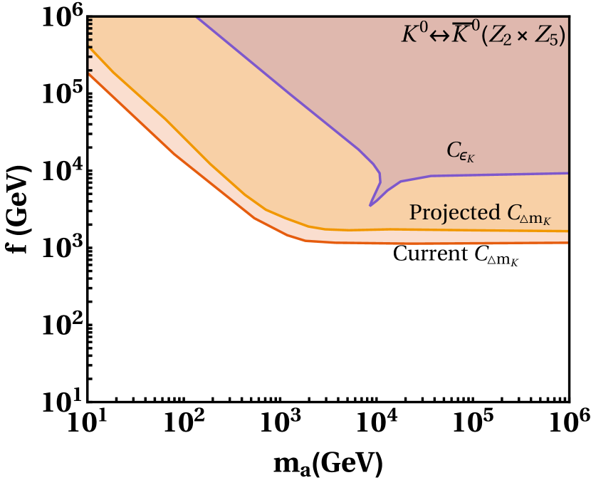
(a)

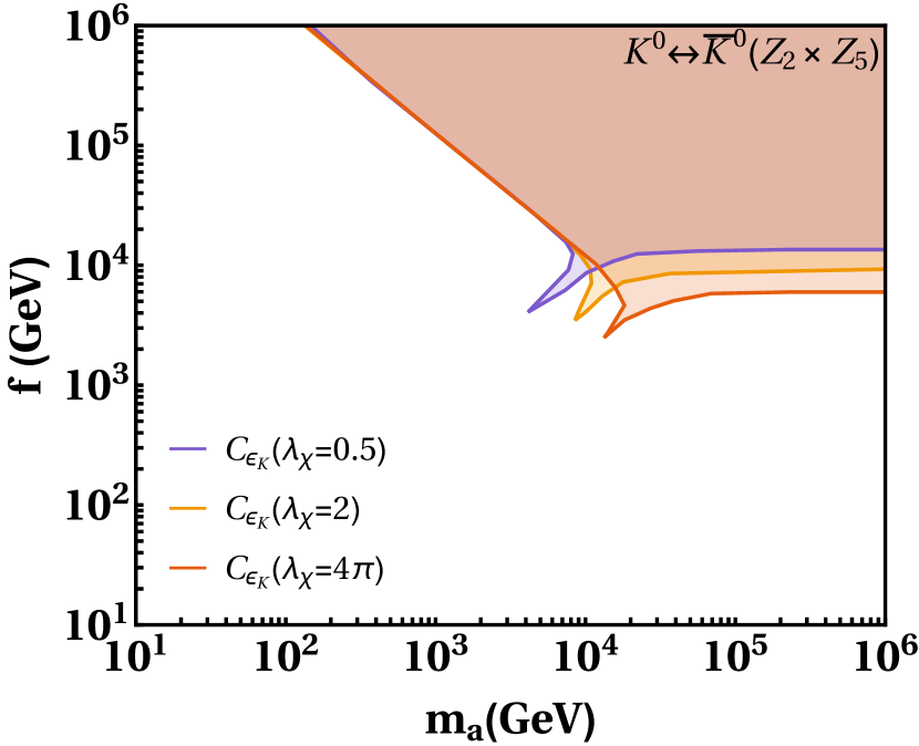
(b)

Figure 1: The allowed parameter space by flavour observables $C_{\epsilon_{K}}$ and $C_{\Delta m_{K}}$ in the $m_{a}-f$ plane for the minimal ($\mathcal{Z}_{2}\times\mathcal{Z}_{5}$) flavour symmetry. On the left panel in figure 1(a), the allowed bounds for $\lambda_{\chi}=2$ with current limits for $C_{\Delta m_{K}}$ and $C_{\epsilon_{K}}$ are shown by red and violet boundaries, respectively. Also, the allowed bound with projected limits of $C_{\Delta m_{K}}$ is shown with yellow boundary. The effect of the variation of the quartic coupling $\lambda_{\chi}$ on the observable $C_{\epsilon_{K}}$ is shown on the right panel in figure 1(b).

In figure 1, we show the bounds on the VEV of the flavon and the mass of the pseudo-scalar flavon arising due to the neutral kaon mixing observables $C_{\epsilon_{K}}$ and $C_{\Delta m_{K}}$ for the minimal model based on the $\mathcal{Z}_{2}\times\mathcal{Z}_{5}$ flavour symmetry. On the left, the allowed region by the observables $C_{\epsilon_{K}}$ and $C_{\Delta m_{K}}$ is shown for the quartic coupling $\lambda_{\chi}=2$. There is a sudden dip in the allowed parameter space given by $C_{\epsilon_{K}}$ which appears due to a cancellation in the Wilson coefficients $C_{2}^{ij}$ and $\tilde{C}_{2}^{ij}$ when masses of scalar and pseudoscalar flavon become identical. For $C_{\Delta m_{K}}$, this dip is not visible in this plot, and is excluded for the quartic coupling for $\lambda_{\chi}=2$. The region bounded by the yellow curve is the allowed parameter space by the future projected sensitivity as shown in table 7. On the right panel, we show the allowed regions of the parameter space by the observable $C_{\epsilon_{K}}$ for $\lambda_{\chi}=0.5,~{}2,~{}4\pi$. It is observed that the allowed region shrinks as $\lambda_{\chi}$ approaches smaller values.

Similar results for non-minimal model based on the $\mathcal{Z}_{2}\times\mathcal{Z}_{9}$ flavour symmetry are shown in figure 2. The constraints on the allowed parameter space by the neutral kaon mixing observables $C_{\epsilon_{K}}$ and $C_{\Delta m_{K}}$, in this case, are more stringent in comparison to that of the minimal ($\mathcal{Z}_{2}\times\mathcal{Z}_{5}$) flavour symmetry. In particular, we observe that the region with the sudden dip is excluded for the non-minimal model. Moreover, there is no allowed parameter space for the future projected sensitivity of the observable $C_{\Delta m_{K}}$ for the bench-mark values of the couplings given in the appendix. Therefore, we show these bounds for different values ( $|y_{12}^{d}|=1$ and $|y_{21}^{d}|=\pi$) of the couplings which are allowed by a more relaxed fit.

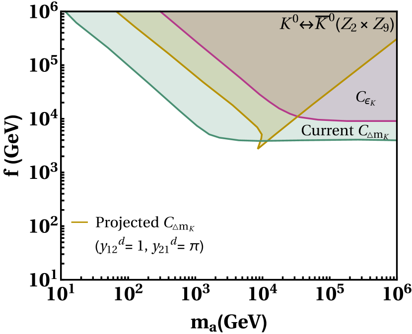
(a)

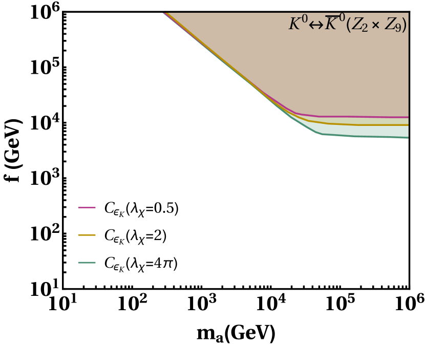
(b)

Figure 2: The allowed parameter space by flavour observables $C_{\epsilon_{K}}$ and $C_{\Delta m_{K}}$ in the $m_{a}-f$ plane for the non-minimal $\mathcal{Z}_{2}\times\mathcal{Z}_{9}$ flavour symmetry. On the left panel in figure 2(a), the allowed bounds for $\lambda_{\chi}=2$ with current limits for $C_{\Delta m_{K}}$ and $C_{\epsilon_{K}}$ are shown by green and magenta boundaries, respectively. Also, the allowed bound with projected limits of $C_{\Delta m_{K}}$ is shown with olive coloured boundary. The effect of the variation of the quartic coupling $\lambda_{\chi}$ on the observable $C_{\epsilon_{K}}$ is shown in the right panel in figure 2(b).

We show the allowed regions of parameter space by the $B_{s}-\bar{B}_{s}$ mixing observables $C_{B_{s}}$ and $\phi_{B_{s}}$ for $\lambda_{\chi}=2$ in the $m_{a}-f$ plane for the minimal model based on the $\mathcal{Z}_{2}\times\mathcal{Z}_{5}$ flavour symmetry and the non-minimal model based on the $\mathcal{Z}_{2}\times\mathcal{Z}_{9}$ flavour symmetry in figure 3. In the left panel in figure 3(a), the red and yellow coloured boundaries are representing allowed flavon contribution for current values of $C_{B_{s}}$ and $\phi_{B_{s}}$, respectively in the minimal model, while that for the non-minimal model are shown in the right panel in figure 3(b), by magenta and green coloured boundaries, respectively. We note that the region in the left panel, bounded by the blue curve, represents the allowed bounds for the observable $C_{B_{s}}$ with projected limits of LHCb Phase-ii@ for the minimal model, while the same for the non-minimal model is shown by the region surrounded by the olive coloured curve in the right panel. For the LHCb phase-i@, the bounds are shown by the pink coloured curves for the minimal as well as for the non-minimal models, which are not appreciably different than that of the LHCb phase-ii@. We also notice an isolated allowed strip of the parameter space for the non-minimal model below the green boundary in the right panel. The effects of the observables $C_{B_{s}}$ and $\phi_{B_{s}}$ are relatively strong in the non-minimal model based on the $\mathcal{Z}_{2}\times\mathcal{Z}_{9}$ flavour symmetry, which is obvious from the figure itself.

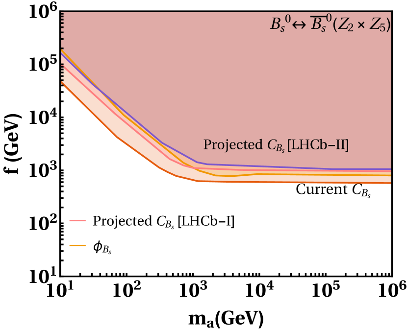
(a)

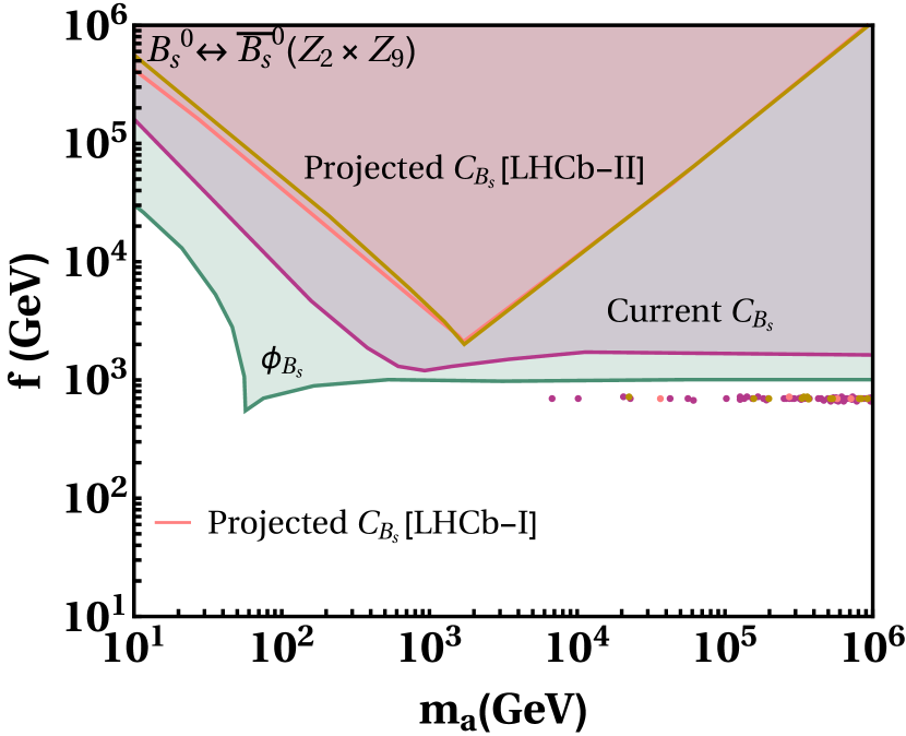
(b)

Figure 3: The parameter space allowed by flavour observables $C_{B_{s}}$ and $\phi_{B_{s}}$ for $\lambda_{\chi}=2$ in the $m_{a}-f$ plane for the minimal ($\mathcal{Z}_{2}\times\mathcal{Z}_{5}$) model in the left panel and for the non-minimal ($\mathcal{Z}_{2}\times\mathcal{Z}_{9}$) model in the right panel.

Figure 4 shows the allowed parameter space by flavour observables $C_{B_{d}}$ and $\phi_{B_{d}}$ of the $B_{d}-\bar{B}_{d}$ mixing for $\lambda_{\chi}=2$ in the $m_{a}-f$ plane. This is shown for the minimal model on the left in figure 4(a) and for the non-minimal model on the right in figure 4(b). In the left panel in figure 4(a) , the red and yellow coloured boundaries are representing allowed flavon contribution for current values of $C_{B_{d}}$ and $\phi_{B_{d}}$, respectively for the minimal model based on the $\mathcal{Z}_{2}\times\mathcal{Z}_{5}$ symmetry while that for non-minimal model is shown in the right panel in figure 4(b) by green and purple coloured boundaries, respectively. Moreover, the region surrounded by the blue curve in the left panel shows the allowed parameter space for the observable $C_{B_{d}}$ with projected limits of LHCb Phase-ii@ for the minimal model while the same for the non-minimal model is shown by olive coloured boundary in the right panel. The bounds for the LHCb phase-i@ are shown by the pink coloured boundaries for the minimal as well as for the non-minimal model, and are very similar to that of the LHCb phase-ii@.

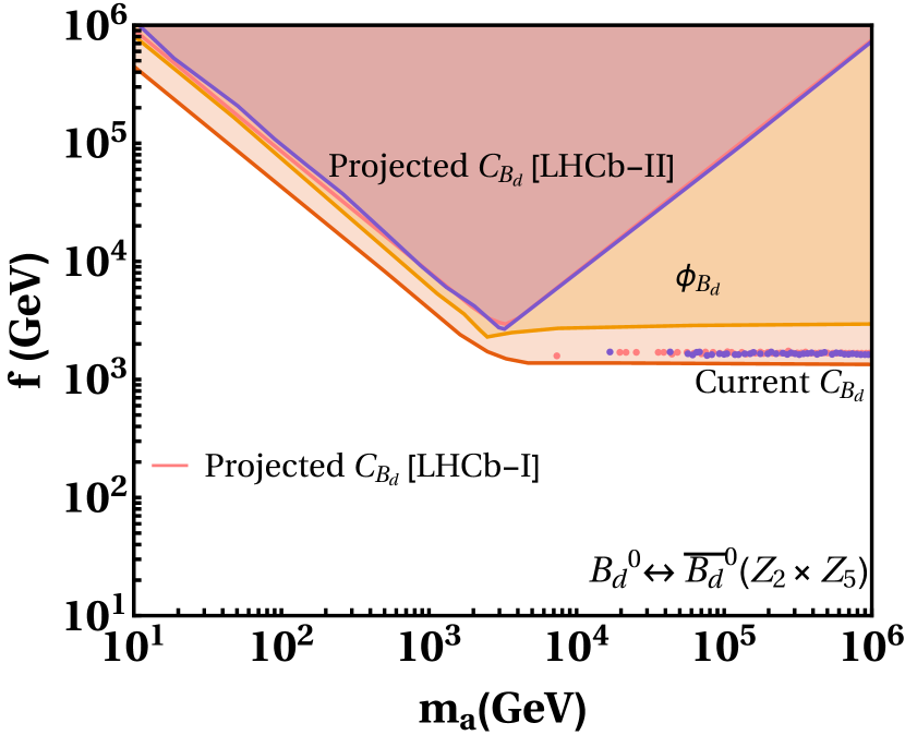
(a)

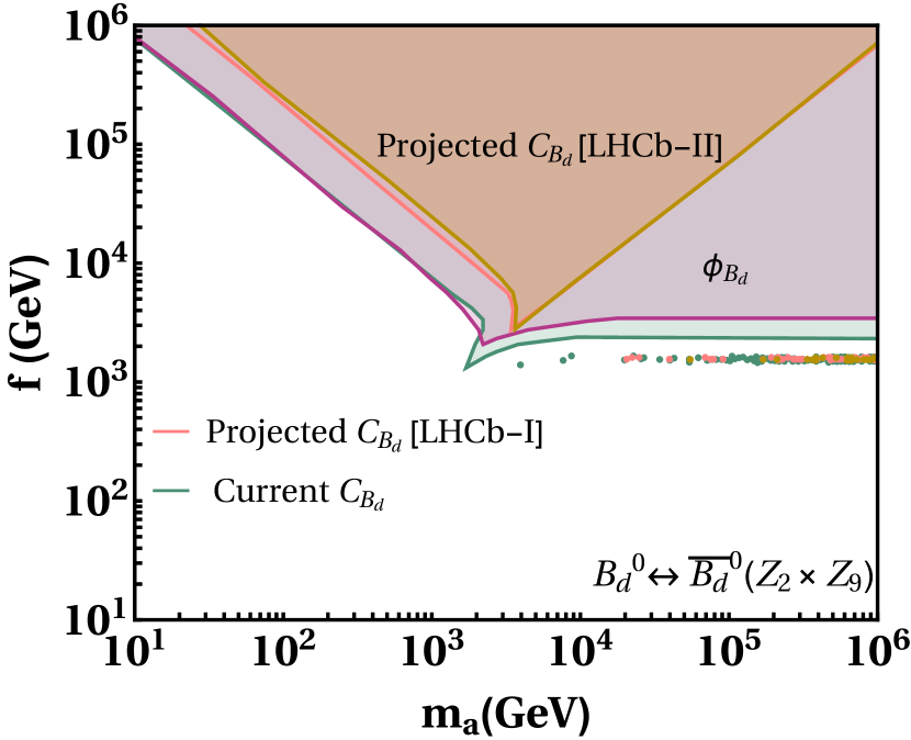
(b)

Figure 4: The allowed parameter space by flavour observables $C_{B_{d}}$ and $\phi_{B_{d}}$ for $\lambda_{\chi}=2$ in the $m_{a}-f$ plane for the minimal ($\mathcal{Z}_{2}\times\mathcal{Z}_{5}$) model in the left panel and for the non-minimal ($\mathcal{Z}_{2}\times\mathcal{Z}_{9}$) model in the right panel.

The SM contribution to $D^{0}-\bar{D}^{0}$ mixing is marred by large hadronic uncertainties. Therefore, for constraining the parameter space of our model, we keep only the flavon contribution to $D^{0}-\bar{D}^{0}$ mixing such that it always lies within the $2\sigma$ experimental bound [53].

$$|M_{12}^{D}|=|\langle D^{0}|\mathcal{H}^{\Delta F=2}|\bar{D}^{0}\rangle|<7.5\times 10^{-3}ps^{-1}$$ (55)

The bound in the $m_{a}-f$ panel arising from the $D^{0}-\bar{D}^{0}$ mixing is shown in figure 5 for the minimal model based on the $\mathcal{Z}_{2}\times\mathcal{Z}_{5}$ flavour symmetry and the non-minimal model based on the $\mathcal{Z}_{2}\times\mathcal{Z}_{9}$ flavour symmetry. The first remarkable observation is the allowed parameter space for the minimal model is much smaller than that of the non-minimal model. This is because the $D^{0}-\bar{D}^{0}$ mixing has an enhancement of the order $\epsilon^{2}$ (see the coupling $2y_{21}^{u}\epsilon^{2}$ in equation 46) in the minimal model based on the $\mathcal{Z}_{2}\times\mathcal{Z}_{5}$ flavour symmetry, which is not present in the case of the non-minimal model. Therefore, the bound derived by the $D^{0}-\bar{D}^{0}$ mixing is the most stringent bound among the bounds given by the mixing observables in the minimal model. However, this is not the case for the non-minimal model.

The one-loop contribution to this mixing from the box diagram depends on the relatively large $y_{ct}$ and $y_{tc}$ couplings of the flavon to fermions. In the minimal model, $y_{tc}$ is zero. Thus, this contribution is proportional to $\epsilon^{4}/(4\pi^{2}f^{2})$ in the minimal model and proportional to $\epsilon^{16}/(4\pi^{2}f^{2})$ in the non-minimal model. Therefore, this contribution is highly suppressed with respect to the tree-level contribution used in deriving the bounds in figure 5.

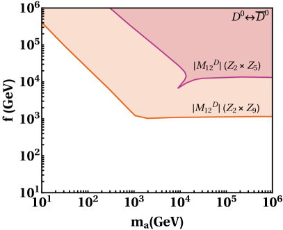
Figure 5: The allowed parameter space by $|M_{12}^{D}|$ for $\lambda_{\chi}=2$ in the $m_{a}-f$ plane for the minimal ($\mathcal{Z}_{2}\times\mathcal{Z}_{5}$) model is shown by the magenta coloured boundary while that for the non-minimal ($\mathcal{Z}_{2}\times\mathcal{Z}_{9}$) model is shown by the red coloured boundary.

5.2 Leptonic decays of mesons

The effective Hamiltonian for flavon mediated decays of neutral mesons into two charged leptons can be written as,

$$\mathcal{H}_{\text{eff}}=-\frac{G_{F}^{2}m_{W}^{2}}{\pi^{2}}\,\left(C_{S}^{ij}\,(\bar{q}_{i}P_{L}q_{j})\bar{\ell}\ell+\tilde{C}_{S}^{ij}\,(\bar{q}_{i}P_{R}q_{j})\bar{\ell}\ell+C_{P}^{ij}(\bar{q}_{i}P_{L}q_{j})\bar{\ell}\gamma_{5}\ell+\tilde{C}_{P}^{ij}(\bar{q}_{i}P_{R}q_{j})\bar{\ell}\gamma_{5}\ell\right)+\text{H.c.}.$$ (56)

The branching ratio of a meson decaying to two charged leptons reads,

$$\text{BR}(M\rightarrow\ell^{+}\ell^{-})= \frac{G_{F}^{4}m_{W}^{4}}{8\pi^{5}}\beta\,m_{M}f_{M}^{2}m_{\ell}^{2}\tau_{M}$$

$$\left(\left|\frac{m_{M}^{2}\big{(}C_{P}^{ij}-\tilde{C}^{ij}_{P}\big{)}}{2m_{\ell}(m_{i}+m_{j})}-C_{A}^{\text{SM}}\right|^{2}+\left|\frac{m_{M}^{2}\big{(}C_{S}^{ij}-\tilde{C}^{ij}_{S}\big{)}}{2m_{\ell}(m_{i}+m_{j})}\right|^{2}\beta^{2}\right)\;,$$ (57)

where $\beta(x)=\sqrt{1-4x^{2}}$ with $x=m_{\ell}/m_{M}$.

The Wilson coefficients having tree-level contribution of the flavon are given as [47, 48],

$$C_{S}^{ij} =\frac{\pi^{2}}{2G_{F}^{2}m_{W}^{2}}\frac{2y_{\ell\ell}y_{ji}}{m_{s}^{2}}$$

$$\tilde{C}_{S}^{ij} =\frac{\pi^{2}}{2G_{F}^{2}m_{W}^{2}}\frac{2y_{\ell\ell}y_{ij}}{m_{s}^{2}}$$

$$C_{P}^{ij} =\frac{\pi^{2}}{2G_{F}^{2}m_{W}^{2}}\frac{2y_{\ell\ell}y_{ji}}{m_{a}^{2}}$$

$$\tilde{C}_{P}^{ij} =\frac{\pi^{2}}{2G_{F}^{2}m_{W}^{2}}\frac{2y_{\ell\ell}y_{ij}}{m_{a}^{2}}\;.$$ (58)

In the SM, processes of mesons decaying to two charged leptons are induced by one-loop contribution, and for the $B_{s}$ meson it is given by[48],

$$C_{A}^{\text{SM}}=-V_{tb}^{*}V_{ts}\,Y\left(\frac{m_{t}^{2}}{m_{W}^{2}}\right)-V_{cb}^{*}V_{cs}\,Y\left(\frac{m_{c}^{2}}{m_{W}^{2}}\right)\;,$$ (59)

where Inami-Lim function $Y(x)$ is given by[54],

$$Y(x)=\eta_{\text{QCD}}\frac{x}{8}\left[\frac{4-x}{1-x}+\frac{3x}{(1-x)^{2}}\log x\right],$$ (60)

where $\eta_{\text{QCD}}=1.0113$ includes NLO QCD effects [55]. For $B_{d}$ meson, the SM predictions are obtained by a simple replacement of indices in equation 59.

The average of the branching fraction of $B_{s}\rightarrow\mu^{+}\mu^{-}$ from HFLAV group is [56],

$$\text{BR}(B_{s}\rightarrow\mu^{+}\mu^{-}) =(3.45\pm 0.29)\times 10^{-9}.$$ (61)

The latest measurement of the branching fraction of $B_{d}\rightarrow\mu^{+}\mu^{-}$ is[57, 58],

$$\text{BR}(B_{d}\rightarrow\mu^{+}\mu^{-}) <2.6\times 10^{-10}\,.$$ (62)

As observed in reference [59], due to sizeable width difference, of the $B_{s}$ meson, theoretical branching ratio can be converted to experimental branching ratio by multiplying $(1-y_{s})^{-1}$, where $y_{s}=0.088\pm 0.014$ [60]. This correction is negligible in the case of the $B_{d}$ meson.

Observables	Current	LHCb-i@	LHCb-ii@	CMS	ATLAS
$\text{BR}(B_{s}\rightarrow\mu^{+}\mu^{-})(\times 10^{9})$	$\pm 0.38$	$\pm 0.30$	$\pm 0.16$	$-$	$\pm 0.50$
$\mathcal{R}_{\mu\mu}$	$\sim 70\%$	$\sim 34\%$	$\sim 10\%$	$\sim 21\%$	$-$
$\tau_{\mu\mu}$	$\sim 12\%$	$\pm 0.16$ ps	$\pm 0.04$ ps	$-$	$-$

Table 8: The current and expected experimental precision for rare $B$ decays observables where LHCb-i@ corresponds to $23fb^{-1}$, LHCb-ii@ corresponds to $300fb^{-1}$, CMS and ATLAS correspond to $3ab^{-1}$[61, 62].

In addition to $\text{BR}(B_{s}\rightarrow\mu^{+}\mu^{-})$ branching ratio, the LHCb collaboration has also measured the ratio of the $\text{BR}(B_{d}\rightarrow\mu^{+}\mu^{-})$ and $\text{BR}(B_{s}\rightarrow\mu^{+}\mu^{-})$ branching fractions, $\mathcal{R}_{\mu\mu}$[57, 58]. The CMS has measured the effective lifetime, $\tau_{\mu\mu}$, of the $B_{s}\rightarrow\mu^{+}\mu^{-}$ decay [61]. We note that the ratio $\mathcal{R}_{\mu\mu}$ is an excellent observable to probe the minimal flavour violation[62]. On the other side, the effective lifetime, $\tau_{\mu\mu}$, can be used to discriminate between the contributions due to any possible new scalar and pseudoscalar mediators [62]. The measured value of the ratio of branching fractions, $\mathcal{R}_{\mu\mu}$, is [57, 58],

$$\mathcal{R}_{\mu\mu} = \frac{\text{BR}(B_{d}\rightarrow\mu^{+}\mu^{-})}{\text{BR}(B_{s}\rightarrow\mu^{+}\mu^{-})}=0.039^{+0.030+0.006}_{-0.024-0.004}.$$ (63)

The effective lifetime $\tau_{\mu\mu}$ and the branching fraction of $B_{s}\rightarrow\mu^{+}\mu^{-}$ are also measured by CMS, and are [61],

$$\tau_{\mu\mu} = 1.83^{+0.23+0.04}_{-0.20-0.04}~{}\rm{ps},$$ (64)

$$\text{BR}(B_{s}\rightarrow\mu^{+}\mu^{-}) =3.83^{+0.38+0.19+0.14}_{-0.36-0.16-0.13}\times 10^{-9}.$$ (65)

We have also taken HFLAV measurement average into account for effective lifetime $\tau_{\mu\mu}$, which is [56],

$$\tau_{\mu\mu} = 2.00^{+0.27}_{-0.26}~{}\rm{ps},$$ (66)

with $\text{BR}(B_{s}\rightarrow\mu^{+}\mu^{-})$ given in equation 61.
The current and future sensitivities of these observables are summarized in table 8. The effective lifetime can be written in the following form [63],

$$\tau_{\mu\mu}=\tau_{B_{s}}\frac{(B_{s}\rightarrow\mu^{+}\mu^{-})^{\rm experiment}}{(B_{s}\rightarrow\mu^{+}\mu^{-})^{\rm theory}},$$ (67)

where we have assumed the SM value of the final state dependent observable $\mathcal{A}^{f}_{\Delta\Gamma}=1$ [60].

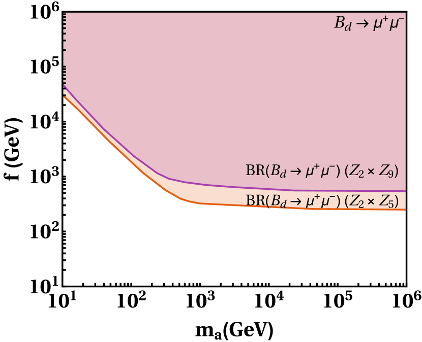
(a)

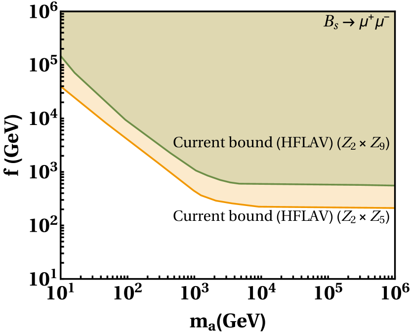
(b)

Figure 6: The allowed parameter space by $\text{BR}(B_{d}\rightarrow\mu^{+}\mu^{-})$ in the left panel and that for the $\text{BR}(B_{s}\rightarrow\mu^{+}\mu^{-})$ in the right panel for $\lambda_{\chi}=2$ with current experimental bounds for the minimal and the non-minimal models.

In figure 6, the bounds coming from the branching ratios $\text{BR}(B_{d}\rightarrow\mu^{+}\mu^{-})$ and the $\text{BR}(B_{s}\rightarrow\mu^{+}\mu^{-})$ for $\lambda_{\chi}=2$ in the $m_{a}-f$ plane are shown. The branching ratios $\text{BR}(B_{d}\rightarrow\mu^{+}\mu^{-})$ and $\text{BR}(B_{s}\rightarrow\mu^{+}\mu^{-})$ place weaker constraints on the parameter space of the minimal model. However, for the non-minimal model, the bounds, particularly from the branching ratios $\text{BR}(B_{s}\rightarrow\mu^{+}\mu^{-})$, are quite stronger. For the projected sensitivities of the LHCb Phase-i@ and ii@ and of the ATLAS for the $\text{BR}(B_{s}\rightarrow\mu^{+}\mu^{-})$, we do not obtain any appreciable improvements in our bounds. Therefore, we do not show them in figure 6.

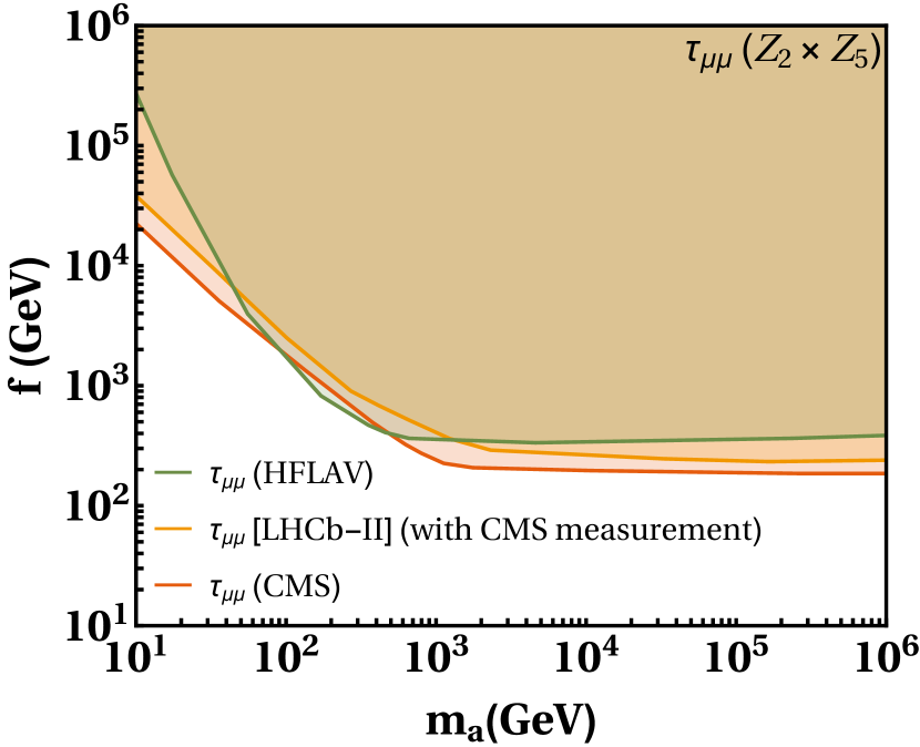
(a)

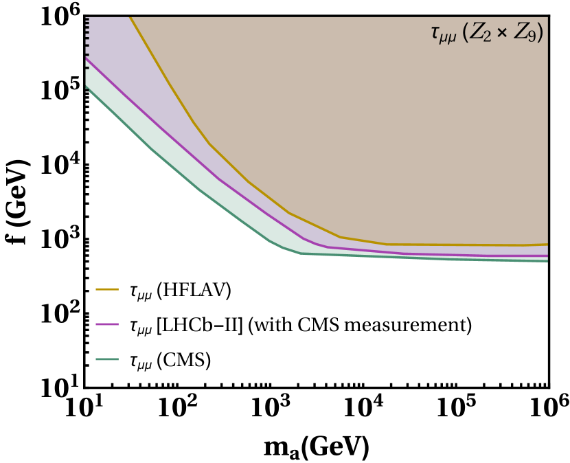
(b)

Figure 7: The allowed parameter space by $\tau_{\mu\mu}$ for $\lambda_{\chi}=2$ in the $m_{a}-f$ plane for the recent measurement and the future projected sensitivity of the LHCb for the minimal ($\mathcal{Z}_{2}\times\mathcal{Z}_{5}$) model on the left, and for the non-minimal ($\mathcal{Z}_{2}\times\mathcal{Z}_{9}$) model on the right.

Figure 7 shows the allowed bounds derived from the HFLAV average of the effective lifetime $\tau_{\mu\mu}$ and the branching-ratio $\text{BR}(B_{s}\rightarrow\mu^{+}\mu^{-})$ by the green coloured curve for the minimal model in figure 7(a) and through the olive coloured boundary for the non-minimal model in figure 7(b). The bounds from the current measurement by CMS, and from the future projected sensitivity of the LHCb phase-ii@ for the minimal model based on $\mathcal{Z}_{2}\times\mathcal{Z}_{5}$, are shown by red and yellow coloured boundaries respectively, in figure 7(a). The same bounds for the non-minimal model based on the $\mathcal{Z}_{2}\times\mathcal{Z}_{9}$ flavour symmetry are shown in figure 7(b) by green and magenta coloured curves respectively. We observe that the bounds are stronger for the non-minimal model in comparison to that of the minimal model. For the projected sensitivity of the LHCb Phase-i@, we do not find any appreciable improvement in the allowed bounds over that from the current measurement. Therefore, we do not show it in figure 7.

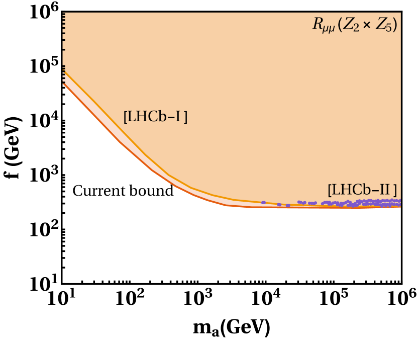
(a)

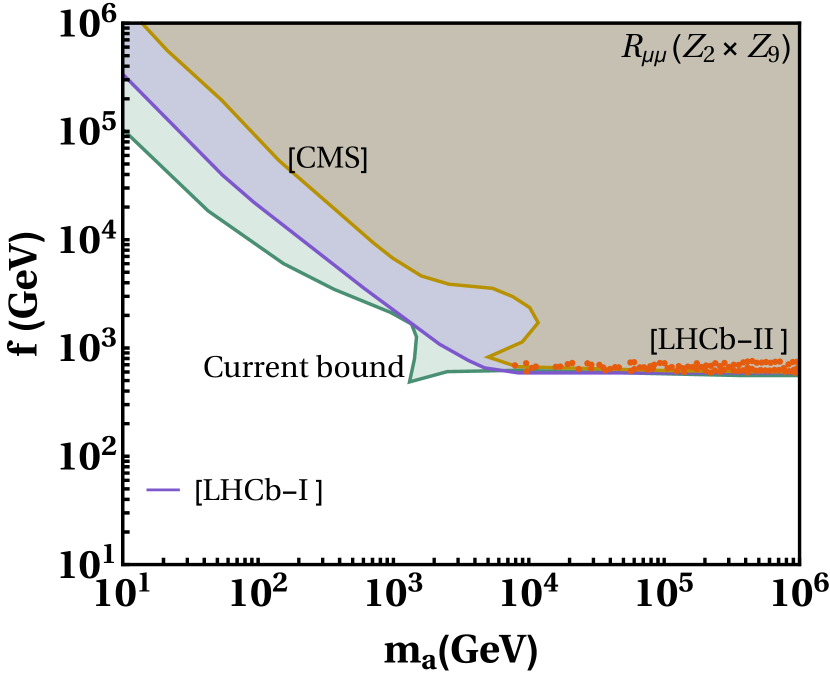
(b)

Figure 8: The left panel represents the allowed parameter space by $\mathcal{R}_{\mu\mu}$ for the minimal ($\mathcal{Z}_{2}\times\mathcal{Z}_{5}$) model with $\lambda_{\chi}=2$ with the current measurement and for the future projected sensitivity of the LHCb Phase-i@ and LHCb Phase-ii@. The same allowed parameter space for the non-minimal ($\mathcal{Z}_{2}\times\mathcal{Z}_{9}$) model is shown in the right panel.

One of the most important observables for our models is the ratio $\mathcal{R}_{\mu\mu}$ whose future projected sensitivity will be crucial to constrain our models. On the left panel in figure 8(a), we show the bounds arising from the ratio $\mathcal{R}_{\mu\mu}$ for the minimal model. These bounds are weaker for the current measurement as well as for the future projected sensitivity of the LHCb Phase-i@ shown by the red and yellow boundaries, respectively. However, the future projected sensitivity of the LHCb Phase-ii@ dramatically changes this scenario and provide extremely stringent constraints on the parameter space of the minimal model shown by the purple coloured strip. Therefore, the LHCb Phase-ii@ will be decisive for the minimal model based on the $\mathcal{Z}_{2}\times\mathcal{Z}_{5}$ flavour symmetry. We also do not find any improvement over the bounds given by the LHCb Phase-i@ using the future projected sensitivity of the CMS experiment. Therefore, we do not show it in figure 8(a).

On the other hand, for the non-minimal model based on the $\mathcal{Z}_{2}\times\mathcal{Z}_{9}$ symmetry, the bounds from the ratio $\mathcal{R}_{\mu\mu}$ are shown in figure 8(b) in the right panel. The bounds from the current measurement are shown by the green boundary while the bounds from the LHCb Phase-i@ are surrounded by the purple coloured curve. Moreover, we also have bounds from the future projected sensitivity of the CMS experiment surrounded by olive coloured boundary. These are more stringent than that of the projected sensitivity of the LHCb Phase-i@ . We note that similar to the minimal model, the bounds for the projected sensitivity of the LHCb Phase-ii@ are highly stringent depicted by the orange coloured strip. This result does not change even if we deviate from the bench-mark values of the Yukawa couplings used for these bounds. Therefore, these bounds are robust, and crucial to test the parameter space of the non-minimal model based on the $\mathcal{Z}_{2}\times\mathcal{Z}_{9}$ symmetry in the future projected sensitivity of the LHCb Phase-ii@.

For the $K_{L}\rightarrow\mu^{+}\mu^{-}$ decay, we have only reliable estimate of the so-called short distance (SD) part of $K_{L}\rightarrow\mu^{+}\mu^{-}$ decay [47]. We use the SM prediction obtained in reference [47] and given by

$$C_{A}^{\text{SM}}=-V_{ts}^{*}V_{td}\,Y\left(\frac{m_{t}^{2}}{m_{W}^{2}}\right)-V_{cs}^{*}V_{cd}Y_{\rm NNL},$$ (68)

where at NNLO $Y_{\rm NNL}=\lambda^{4}P_{c}(Y)$, $\lambda=|V_{us}|$ and $P_{c}(Y)=0.113\pm 0.017$[64]. The short distance contribution can be extracted from the experimental measurement and has an upper limit[48],

$$\text{BR}(K_{L}\rightarrow\mu^{+}\mu^{-})_{\rm SD} <2.5\times 10^{-9}.$$ (69)

For the case of $D\rightarrow\mu^{+}\mu^{-}$ decay, the SM contribution is plagued by large non-perturbative effects. Therefore, we only require that the flavon contribution does not generate more than the experimental upper bound on the branching ratio that is given at $90\%$ C.L.[65],

$$\text{BR}(D\rightarrow\mu^{+}\mu^{-}) <6.2\times 10^{-9}.$$ (70)

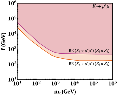
Figure 9: The parameter space allowed by $\text{BR}(K_{L}\rightarrow\mu^{+}\mu^{-})_{\rm SD}$ with $\lambda_{\chi}=2$ in the $m_{a}-f$ plane for the minimal ($\mathcal{Z}_{2}\times\mathcal{Z}_{5}$) and non-minimal ($\mathcal{Z}_{2}\times\mathcal{Z}_{9}$) model are shown with red and magenta coloured boundaries, respectively.

We show bounds arising from the $\text{BR}(K_{L}\rightarrow\mu^{+}\mu^{-})_{\rm SD}$ for $\lambda_{\chi}=2$ for the minimal and the non-minimal models in the $m_{a}-f$ plane in figure 9. It turns out that the constraints on the parameter space of the minimal model are weaker. However, the bounds on the parameter space of the non-minimal model are more stringent. The constraints from the $D\rightarrow\mu^{+}\mu^{-}$ decay are much weaker than that from the $\text{BR}(K_{L}\rightarrow\mu^{+}\mu^{-})_{\rm SD}$. Therefore, we do not show them in this work.

6 Leptonic flavour physics in the minimal and non-minimal $\mathcal{Z}_{2}\times\mathcal{Z}_{N}$ flavour symmetry

Charged lepton flavour violation (CLFV) has a substantial potential to provide bounds on flavon physics in future upcoming experiments. The quark flavour constraints currently dominate our flavon model. However, it is expected that the future projected sensitivities of CLFV, which are shown in table 9, may significantly improve the bounds from quark flavour physics.

Observables	Current sensitivity	Ref.	Future projection	Ref.
BR($\mu\to e\gamma$ )	$<4.2\times 10^{-13}$	MEG [66]	$6\times 10^{-14}$	MEGii@ [67]
BR($\tau\to e\gamma$)	$<3.3\times 10^{-8}$	Babar [68]	$\sim 10^{-9}$	Belle ii@ [69]
BR( $\tau\to\mu\gamma$)	$<4.4\times 10^{-8}$	Babar [68]	$\sim 10^{-9}$	Belle ii@ [69]
BR $\text{(}\mu\to e\text{)}^{\rm Au}$	$<7\times 10^{-13}$	SINDRUM ii@ [70]	$-$	$-$
BR $\text{(}\mu\to e\text{)}^{\rm Al}$	$-$	$-$	$3\times 10^{-15}$	COMET Phase-i@ [71, 72]
BR $\text{(}\mu\to e\text{)}^{\rm Al}$	$-$	$-$	$6\times 10^{-17}$	COMET Phase-ii@ [71]
BR $\text{(}\mu\to e\text{)}^{\rm Al}$	$-$	$-$	$6\times 10^{-17}$	Mu2e [73]
BR $\text{(}\mu\to e\text{)}^{\rm Al}$	$-$	$-$	$3\times 10^{-18}$	Mu2e ii@ [72]
BR $\text{(}\mu\to e\text{)}^{\rm Si}$	$-$	$-$	$2\times 10^{-14}$	DeeMe [74]
BR $\text{(}\mu\to e\text{)}^{\rm Ti}$			$\sim 10^{-20}-10^{-18}$	PRISM/PRIME [75, 76]
BR( $\mu\to e\bar{e}e$)	$<1.0\times 10^{-12}$	SINDRUM [77]	$\sim 10^{-16}$	Mu3e [78]
BR($\tau\to 3\mu$ )	$<$ $2.1\times 10^{-8}$	Belle [79]	$\sim 10^{-9}$	Belle ii@ [69]
BR($\tau\to 3e$ )	$<$ $2.7\times 10^{-8}$	Belle [79]	$\sim 10^{-9}$	Belle ii@ [69]

Table 9: Experimental upper limits on various Leptonic flavour violation (LFV) processes.

6.1 Radiative leptonic decays

The effective Lagrangian for the radiative leptonic decays can be written as,

$$\mathcal{L}_{\text{eff}} =m_{\ell^{\prime}}\,C_{T}^{L}\,\bar{\ell}\sigma^{\rho\lambda}P_{L}\,\ell^{\prime}\,F_{\rho\lambda}+m_{\ell^{\prime}}\,C_{T}^{R}\,\bar{\ell}\sigma^{\rho\lambda}P_{R}\,\ell^{\prime}\,F_{\rho\lambda}.$$ (71)

The radiative leptonic decays are mediated by dipole operators and their branching ratio reads,

$$\text{BR}(\ell^{\prime}\rightarrow\ell\gamma)=\frac{m_{\ell^{\prime}}^{5}}{4\pi\Gamma_{\ell^{\prime}}}\left(|C_{T}^{L}|^{2}+|C_{T}^{R}|^{2}\right)\;.$$ (72)

The one-loop contribution to the radiative leptonic decays is shown in figure 10. The corresponding Wilson coefficients are [28],

$$C_{T}^{L}=(C_{T}^{R})^{*}=\frac{e}{32\pi^{2}}\sum_{k=e,\mu,\tau} \bigg{\{}\frac{1}{6}\left(\,y^{*}_{\ell k}y_{\ell^{\prime}k}+\frac{m_{\ell}}{m_{k}}y^{*}_{k\ell}y_{k\ell^{\prime}}\right)\left(\frac{1}{m_{s}^{2}}-\frac{1}{m_{a}^{2}}\right)$$

$$-y_{\ell k}y_{k\ell^{\prime}}\frac{m_{k}}{m_{\ell^{\prime}}}\left[\frac{1}{m_{s}^{2}}\left(\frac{3}{2}+\log\frac{m_{\ell^{\prime}}^{2}}{m_{s}^{2}}\right)-\frac{1}{m_{a}^{2}}\left(\frac{3}{2}+\log\frac{m_{\ell^{\prime}}^{2}}{m_{a}^{2}}\right)\right]\bigg{\}}\;.$$ (73)

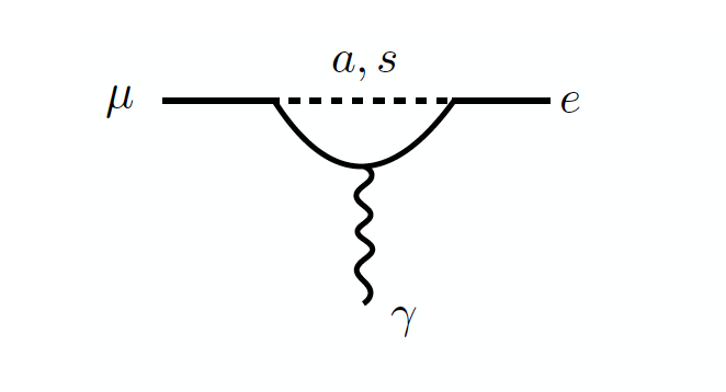
Figure 10: Feynman diagram representing $\mu\rightarrow e\gamma$ decay.

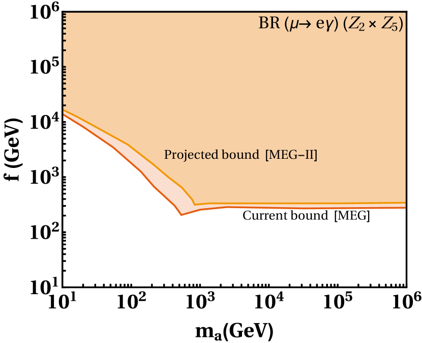
(a)

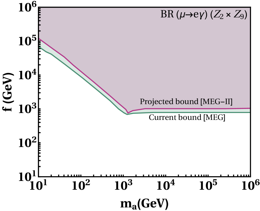
(b)

Figure 11: In the left panel, the red and yellow coloured boundaries represent the allowed parameter space by the current and projected sensitivities of the MEG experiment on the $\text{BR}(\mu\rightarrow e\gamma)$ for the minimal ($\mathcal{Z}_{2}\times\mathcal{Z}_{5}$) model with $\lambda_{\chi}=2$ in the $m_{a}-f$ plane. The same bounds for the non-minimal ($\mathcal{Z}_{2}\times\mathcal{Z}_{9}$) model are shown in the right panel with green and magenta coloured curves, respectively .

The radiative leptonic decays $\mu\rightarrow e\gamma$ places weak constraints on the parameter space of the minimal model as shown in figure 11(a). This does not change much even for the future projected sensitivities of the MEG-ii@ experiment. For the non-minimal model, the bounds from the current measurement of the MEG experiment, shown in figure 11(b) by the green boundary, are quite stringent relative to that of the minimal model. Moreover, for the future projected sensitivities of the MEGii@ experiment, the constraints are further stronger depicted by the magenta coloured boundary. The constraints coming from the decays $\tau\rightarrow e\gamma$ and $\tau\rightarrow\mu\gamma$ are weaker than that of the decay $\mu\rightarrow e\gamma$. Therefore, they are not shown in this work.

6.2 $A~{}\mu\rightarrow A~{}e$ conversion

The effective Lagrangian describing $A~{}\mu\rightarrow A~{}e$ conversion can be written as,

$$\mathcal{L}_{\text{eff}}=C_{qq}^{VL}\,\bar{e}\gamma^{\nu}P_{L}\mu\,\bar{q}\gamma_{\nu}q+m_{\mu}m_{q}\,C_{qq}^{SL}\bar{e}P_{R}\mu\,\bar{q}q+m_{\mu}\alpha_{s}C_{gg}^{L}\,\bar{e}P_{R}\mu\,G_{\rho\nu}G^{\rho\nu}\,+(R\leftrightarrow L)\;,$$ (74)

Moreover, there is additional contribution to $A~{}\mu\rightarrow A~{}e$ conversion from the dipole operators given in equation (71).

The Feynman diagram for $A~{}\mu\rightarrow A~{}e$ conversion is shown in figure 12. The corresponding Wilson coefficients arise due to the diagram on the left in figure 12 [28],

$$C^{SL}_{qq} =\left(\frac{1}{m_{s}^{2}}+\frac{1}{m_{a}^{2}}\right)y_{\mu e}^{*}\text{Re}(y_{qq})\,,$$

$$C^{SR}_{qq} =\left(\frac{1}{m_{s}^{2}}-\frac{1}{m_{a}^{2}}\right)y_{e\mu}\text{Re}(y_{qq})\,.$$ (75)

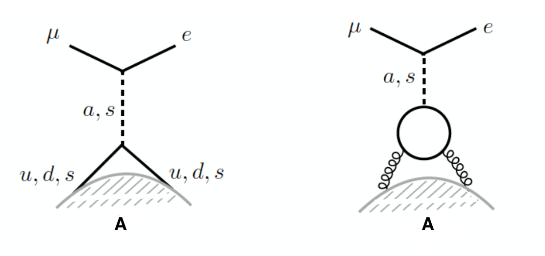
Figure 12: Feynman diagram showing $A~{}\mu\rightarrow A~{}e$ conversion.

The nuclear effects which include effects of quarks inside the nucleons as well as the contribution of the Feynman diagram on the right side of figure 12 are absorbed in the nucleon-level Wilson coefficients defined by,

$$\tilde{C}_{p}^{VL} =\sum_{q=u,d}C^{VL}_{qq}\,f_{V_{q}}^{p},$$ (76)

$$\tilde{C}_{p}^{SL} =\sum_{q=u,d,s}C^{SL}_{qq}\,f_{q}^{p}-\sum_{Q=c,b,t}C^{SL}_{QQ}\,f_{\text{heavy}}^{p}\,,$$

where the quark content of the proton is accounted by vector and scalar couplings $f_{V_{q}}^{p},f_{q}^{p}$, and $f_{\text{heavy}}^{p}=2/27\big{(}1-f_{u}^{p}-f_{d}^{p}-f_{s}^{p}\big{)}$ [80]. For right-handed operators, analogous expressions are obtained by replacing $L$ with $R$, and for the neutron $p$ is replaced by $n$. The vector operators contribute extremely less than the scalar operators and can be neglected [28]. The numerical values of vector and scalar couplings are taken from references [81, 82], which are based on the lattice average given in reference [83],

$$f_{u}^{p} =0.0191\qquad\qquad f_{u}^{n}=0.0171\,,$$

$$f_{d}^{p} =0.0363\qquad\qquad f_{d}^{n}=0.0404\,,$$

$$f_{s}^{p} =f_{s}^{n}=0.043\,.$$ (77)

The $A~{}\mu\rightarrow A~{}e$ conversion rate including nuclear effects can be written as[28],

$$\Gamma_{A~{}\mu\rightarrow A~{}e}=\frac{m_{\mu}^{5}}{4}\left|C_{T}^{L}D+4\left[m_{\mu}m_{p}\tilde{C}_{p}^{SL}+\tilde{C}_{p}^{VL}V^{p}+(p\rightarrow n)\right]\right|^{2}\,+L\rightarrow R,$$ (78)

where the dimensionless coefficients $D,S^{p,n}$ and $V^{p,n}$ depend on the overlap integrals of the initial state muon and the final-state electron wave-functions with the target nucleus, and their numerical values are given in table 10 [84],

Target	$D$	$S^{p}$	$S^{n}$	$V^{p}$	$V^{n}$	$\Gamma_{\text{capt}}[10^{6}\text{s}^{-1}]$
Au	0.189	0.0614	0.0918	0.0974	0.146	13.06
Al	0.0362	0.0155	0.0167	0.0161	0.0173	0.705
Si	0.0419	0.0179	0.0179	0.0187	0.0187	0.871
Ti	0.0864	0.0368	0.0435	0.0396	0.0468	2.59

Table 10: Numerical values of the dimensionless coefficients $D,S^{p,n}$, $V^{p,n}$ and the muon capture rate for different nuclei.

where $\Gamma_{\text{capt}}$ stands for the muon capture rate.

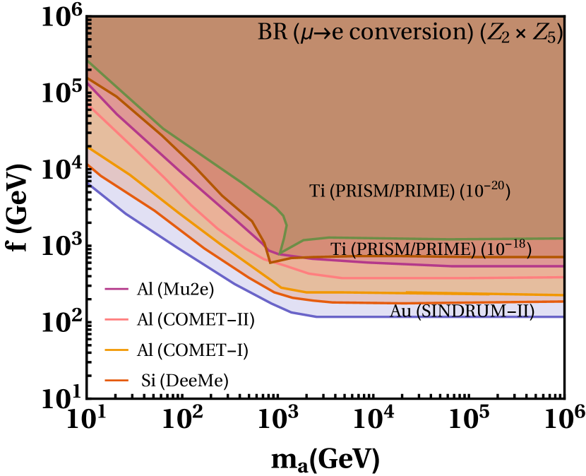
(a)

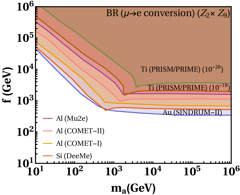
(b)

Figure 13: The left panel represents the allowed parameter space by $\text{BR}(\mu\rightarrow e)$ conversion in the $m_{a}-f$ plane with different experimental limits of various target nuclei in table 9 with $\lambda_{\chi}=2$, for the minimal ($\mathcal{Z}_{2}\times\mathcal{Z}_{5}$) model. Similar allowed parameter space for the non-minimal ($\mathcal{Z}_{2}\times\mathcal{Z}_{9}$) model is shown in the right panel.

The bounds from $\text{BR}(\mu\rightarrow e)$ conversion for different target nucleus with $\lambda_{\chi}=2$ in the $m_{a}-f$ plane are shown in figure 13. The bounds for the minimal model are shown in figure 13(a) for the current measurement and for the different future projected sensitivities, and the same for the non-minimal model are shown in figure 13(b). The strongest bounds among them arise from the projected future sensitivities of the PRISM/PRIME experiment for the minimal as well as non-minimal models.

6.3 $\mu\rightarrow 3e$ and $\tau\rightarrow 3\mu$ decays

The three body flavour violating leptonic decays $\mu\to 3e$ and $\tau\to 3\ell$ where $\ell=e,\mu$ provide additional tests of the dipole operators given in equation (71). Their decay width can be written as[28],

$$\Gamma(\ell^{\prime}\rightarrow 3\ell)=\frac{\alpha m_{\ell}^{\prime 5}}{12\pi^{2}}\left|log\frac{{m_{\ell}^{\prime}}^{2}}{{m_{\ell}}^{2}}-\frac{11}{4}\right|\left(|C_{T}^{L}|^{2}+|C_{T}^{R}|^{2}\right).$$ (79)

where the tree-level contribution is ignored due to the strong chiral-suppression which is dominated by the logarithmic enhancement of the dipole operators[28]. Other contributions, such as $Z$-mediated penguin are strongly suppressed and ignored[85].

(a)

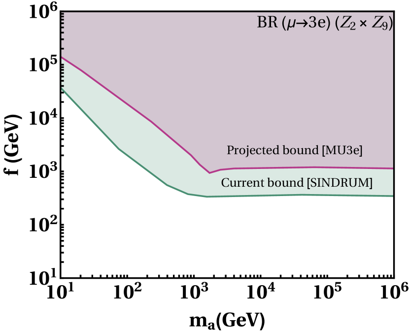
(b)

Figure 14: The allowed parameter space by $\text{BR}(\mu\rightarrow 3e)$ for the minimal ($\mathcal{Z}_{2}\times\mathcal{Z}_{5}$) model on the left and for the non-minimal ($\mathcal{Z}_{2}\times\mathcal{Z}_{9}$) model on the right with $\lambda_{\chi}=2$.

In figure 14, we show the allowed parameter space by $\text{BR}(\mu\rightarrow 3e)$ for $\lambda_{\chi}=2$ in the $m_{a}-f$ plane. For the minimal model, the bounds are shown in figure 14(a). They are weaker for the current measurement and for the future projected sensitivity as well. In figure 14(b), the same bounds on the allowed parameter space are shown for the non-minimal model. For the current measurement, the bound is given by the green boundary, and for the future projected sensitivity, it is depicted by the magenta coloured curve. As obvious from figure 14(b), the bounds for the non-minimal model are quite stringent relative to the minimal model. The bounds from the decay $\tau\to 3\ell$ are much weaker and are not shown in this work.

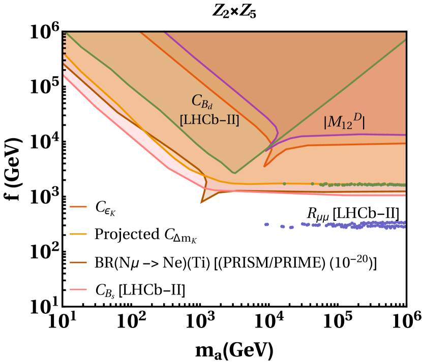
(a)

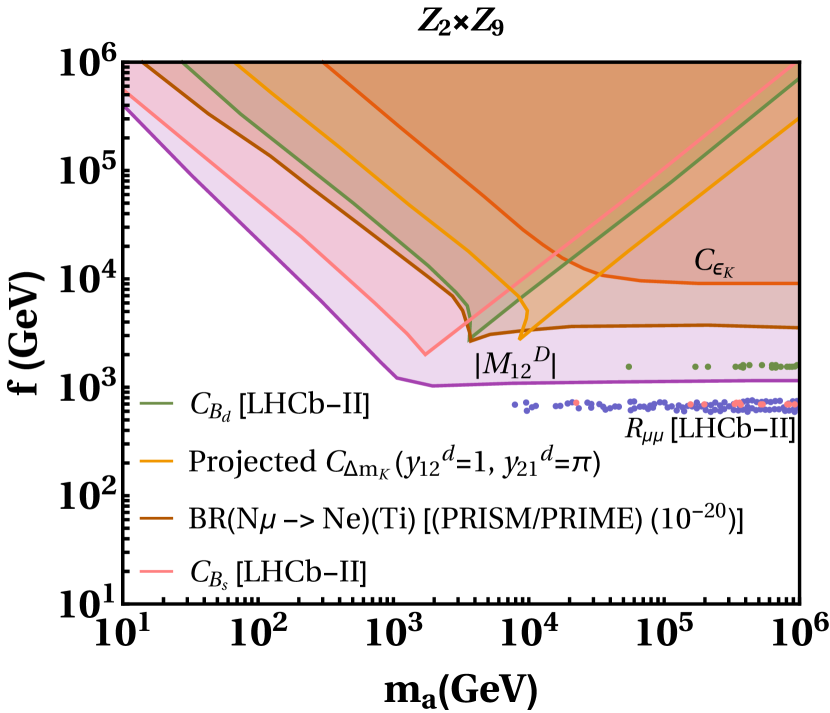
(b)

Figure 15: Summarized significant bounds on the minimal $\mathcal{Z}_{2}\times\mathcal{Z}_{5}$ and the non-minimal $\mathcal{Z}_{2}\times\mathcal{Z}_{9}$ model in the left and the right panel respectively.

Finally, we show a summary of the most relevant and stringent bounds on the prameter space of the minimal and the non-minimal models in figure 15.

7 Summary

We have discussed a simple FN mechanism in the framework of a new $\mathcal{Z}_{2}\times\mathcal{Z}_{N}$ flavour symmetry. This symmetry is inspired by the extensively explored 2HDM and the MSSM, where the $\mathcal{Z}_{2}$ symmetry is an essential ingredient of the theoretical framework. We show that a minimal form of this symmetry, the $\mathcal{Z}_{2}\times\mathcal{Z}_{5}$, is capable of providing an explanation to the charged fermion mass pattern and quark mixing along with a mechanism to predict neutrino masses and mixing angles. However, for the minimal model based on the $\mathcal{Z}_{2}\times\mathcal{Z}_{5}$ flavour symmetry, all the Yukawa couplings are not order one, which is a preferred choice in literature. This observation leads to a non-minimal model based on the $\mathcal{Z}_{2}\times\mathcal{Z}_{9}$ flavour symmetry, where all the couplings are order one. The FN mechanism created through the $\mathcal{Z}_{2}\times\mathcal{Z}_{N}$ flavour symmetry is different from the conventional FN mechanism, where a continuous $U(1)$ symmetry is employed to achieve a solution of the flavour problem of the SM.

The leading question is the scale where the flavour symmetry $\mathcal{Z}_{2}\times\mathcal{Z}_{N}$ is broken. This is addressed by deriving the bounds on the parameter space of the model using flavour physics data. Moreover, future sensitivities of the CMS and the phase-i@ and ii@ of the LHCb for the flavour physics observables turn out to be an interesting and fertile ground to investigate the breaking scale of the $\mathcal{Z}_{2}\times\mathcal{Z}_{N}$ flavour symmetry. Particularly the reach of the experiments such as MEG ii@ and PRISM/PRIME, which are going to test lepton flavour violating effects, could play a crucial role in improving the present limits by orders of magnitude.

For the minimal model based on the flavour symmetry $\mathcal{Z}_{2}\times\mathcal{Z}_{5}$, the quark flavour physics plays a crucial role. For instance, the most stringent constraints on the parameter space of the minimal model comes from the $K^{0}-\bar{K}^{0}$ and $D^{0}-\bar{D}^{0}$ mixing using the present data. In particular, the $D^{0}-\bar{D}^{0}$ provides the very tight bounds since it is highly unsuppressed due to the PMS in the minimal model. The $B_{d}-\bar{B}_{d}$ mixing provides tighter bounds than the $B_{s}-\bar{B}_{s}$ mixing. The future projected sensitivity of the $B_{d}-\bar{B}_{d}$ mixing will further constrain the parameter space of the minimal model in future. The rare decays $\text{BR}(B_{d,s}\rightarrow\mu^{+}\mu^{-})$ branching ratios place relatively weaker bounds on the parameter space of the minimal model for the present measurements as well as for the future projected sensitivities of phase-i@ and ii@ of the LHCb. However, the future projected sensitivity of the rare $B$ decays observable $\mathcal{R}_{\mu\mu}$ provides robust and the most stringent bound on the parameter space of the minimal model. Among the leptonic observables, the future projected sensitivity of the PRISM/PRIME for the BR $\text{(}\mu\to e\text{)}^{\rm Ti}$ will substantially be able to constrain the parameter space of the minimal model.

In the case of the non-minimal model based on the flavour symmetry $\mathcal{Z}_{2}\times\mathcal{Z}_{9}$, both the quark as well as leptonic flavour physics play decisive role in constraining the parameter space of the non-minimal model. On the quark flavour side, the most stringent bounds are coming from the $K^{0}-\bar{K}^{0}$ mixing while from the leptonic flavour side, it comes from the radiative leptonic decay $\mu\rightarrow e\gamma$. We observe that every flavour observable including the branching ratio of the $K_{L}\rightarrow\mu^{+}\mu^{-}$ decay, is able to provide important bounds on the parameter space of the non-minimal model. In particular, the future projected sensitivity of the rare $B$ decays observable $\mathcal{R}_{\mu\mu}$ for the LHCb and CMS experiments, will test the non-minimal model rigorously. Moreover, the future projected sensitivity of the PRISM/PRIME for the BR $\text{(}\mu\to e\text{)}^{\rm Ti}$ will eliminate a large part of the allowed parameter space.

In short, quark flavour physics will determine the allowed parameter space of the minimal model, and leptonic flavour violating observables independently can further probe the parameter space upto a very high scale. For the non-minimal model based on the $\mathcal{Z}_{2}\times\mathcal{Z}_{9}$ flavour symmetry, quark and lepton flavour physics play a crucial role in constraining the allowed parameter space of the model. The future sensitivities of the experiments such as MEG ii@, Mu3e, DeeMe, COMET, Mu2e and PRISM/PRIME will be able to constrain the parameter space of the non-minimal model based on the $\mathcal{Z}_{2}\times\mathcal{Z}_{9}$ flavour symmetry. On the quark side, the $B_{d}-\bar{B}_{d}$ mixing in the future phase-i@ and ii@ of the LHCb will be able to eliminate a sufficient region of the parameter space. In future phase-ii@ of the LHCb, the ratio $\mathcal{R}_{\mu\mu}$ will be crucial in ruling out the major part of the flavon parameter space. Thus, future projected sensitivities of the LHCb phase-i@ and ii@ will play a defining role in determining the fate of the flavon models discussed in this work.

Appendix

Benchmark points for the Yukawa couplings

We reproduce the fermion masses using the following values of the fermion masses at $1$TeV[86],

$$\{m_{t},m_{c},m_{u}\} \simeq \{150.7\pm 3.4,~{}0.532^{+0.074}_{-0.073},~{}(1.10^{+0.43}_{-0.37})\times 10^{-3}\}~{}{\rm GeV},$$

$$\{m_{b},m_{s},m_{d}\} \simeq \{2.43\pm 0.08,~{}4.7^{+1.4}_{-1.3}\times 10^{-2},~{}2.50^{+1.08}_{-1.03}\times 10^{-3}\}~{}{\rm GeV},$$

$$\{m_{\tau},m_{\mu},m_{e}\} \simeq \{1.78\pm 0.2,~{}0.105^{+9.4\times 10^{-9}}_{-9.3\times 10^{-9}},~{}4.96\pm 0.00000043\times 10^{-4}\}~{}{\rm GeV}.$$ (80)

The magnitudes and phases of the CKM mixing elements are [38],

$$|V_{ud}| = 0.97370\pm 0.00014,|V_{cb}|=0.0410\pm 0.0014,|V_{ub}|=0.00382\pm 0.00024,$$ (81)

$$\sin 2\beta = 0.699\pm 0.017,~{}\alpha=(84.9^{+5.1}_{-4.5})^{\circ},~{}\gamma=(72.1^{+4.1}_{-4.5})^{\circ},\delta=1.196^{+0.045}_{-0.043}$$

The present scenario of the neutrino physics for the normal hierarchy can be described by the following global fit results[87],

$$\Delta m_{21}^{2} = (7.55^{+0.59}_{-0.5})\times 10^{-5}{\rm eV}^{2},|\Delta m_{31}^{2}|=(2.50\pm 0.09)\times 10^{-3}\rm{eV}^{2},$$ (82)

$$\sin^{2}\theta_{12} = (3.20^{+0.59}_{-0.47})\times 10^{-1},\sin^{2}\theta_{23}=(5.47^{+0.52}_{-1.02})\times 10^{-1},\sin^{2}\theta_{13}=(2.160^{+0.25}_{-0.20})\times 10^{-2},$$

where range of errors is $3\sigma$.

We fit quark and charged-lepton masses along with the neutrino oscillation data by defining

$$\chi^{2}=\dfrac{(m_{q}-m_{q}^{\rm{model}})^{2}}{\sigma_{m_{q}}^{2}}+\dfrac{(m_{\ell}-m_{\ell}^{\rm{model}})^{2}}{\sigma_{m_{\ell}}^{2}}+\dfrac{(\sin\theta_{ij}-\sin\theta_{ij}^{\rm{model}})^{2}}{\sigma_{\sin\theta_{ij}}^{2}}+\dfrac{(\sin 2\beta-\sin 2\beta^{\rm{model}})^{2}}{\sigma_{\sin 2\beta}^{2}}+\dfrac{(\alpha-\alpha^{\rm{model}})^{2}}{(\sigma_{\alpha})^{2}}\\ +\dfrac{(\gamma-\gamma^{\rm{model}})^{2}}{(\sigma_{\gamma})^{2}}+\dfrac{(\Delta m_{21}^{2}-\Delta m_{21}^{2~{}\rm{model}})}{\sigma_{\Delta m_{21}^{2}}^{2}}+\dfrac{(\Delta m_{31}^{2}-\Delta m_{31}^{2~{}\rm{model}})}{\sigma_{\Delta m_{31}^{2}}^{2}}+\dfrac{(\sin\theta_{ij}^{\nu}-\sin\theta_{ij}^{\nu~{}\rm{model}})^{2}}{\sigma_{\sin\theta_{ij}^{\nu}}}$$

where $q=\{u,d,c,s,t,b\}$, $\ell=\{e,\mu,\tau\}$, $\nu=\{\nu_{e},\nu_{\mu},\nu_{\tau}\}$ and $i,j=1,2,3$. The phases of the CKM matrix in the standard choice are defined as follows:

$$\beta^{\text{model}}=\text{arg}\left(-\dfrac{V_{cd}V_{cb}^{*}}{V_{td}V_{tb}^{*}}\right),~{}\alpha^{\text{model}}=\text{arg}\left(-\dfrac{V_{td}V_{tb}^{*}}{V_{ud}V_{ub}^{*}}\right),~{}\gamma^{\text{model}}=\text{arg}\left(-\dfrac{V_{ud}V_{ub}^{*}}{V_{cd}V_{cb}^{*}}\right).$$ (83)

The minimal model

The dimensionless coefficients $y_{ij}^{u,d,\ell,\nu}=|y_{ij}^{u,d,\ell,\nu}|e^{i\phi_{ij}^{q,\ell,\nu}}$ are scanned with $|y_{ij}^{u,d,\ell,\nu}|\in[0.1,4\pi]$ and $\phi_{ij}^{q,\ell,\nu}\in[0,2\pi]$. The fit results are,

$$Y_{u}=\begin{pmatrix}-1.68-3.37i&-0.09+0.03i&-0.1-0.02i\\ 1.53+4.95i&-0.57+0.55i&0.48+0.002i\\ 0.76+0.18i&-1.04+0.46i&0.58-0.65i\end{pmatrix},$$

$$Y_{d}=\begin{pmatrix}-4.15+3.58i&2.20-0.89i&2.62-4.20i\\ -0.33-0.36i&0.07-0.075i&0.17+0.47i\\ -0.24-0.07i&-0.06-0.084i&-0.07-0.12i\end{pmatrix},$$

$$Y_{l}=\begin{pmatrix}-0.07-0.06i&0.099-0.004i&0.45-0.32i\\ -0.14-0.09i&0.08-0.06i&-0.63+0.24i\\ -0.04+0.09i&-0.09+0.06i&0.10-0.0003i\end{pmatrix},$$

with $\epsilon=0.1$ $\epsilon^{\prime}=1.259\times 10^{-13}$ , $\chi^{2}\approx 14$, and the following results for neutrino oscillation data,

$$\{|y_{11}^{\nu}|,|y_{22}^{\nu}|,|y_{33}^{\nu}|,|c_{11}|,|c_{22}|,|c_{33}|\} \simeq \{3.14,3.14,1.48,3.14,0.90,2.76\},$$

$$\{\phi_{11}^{\nu},\phi_{22}^{\nu},\phi_{33}^{\nu},\phi_{11}^{c},\phi_{22}^{c},\phi_{33}^{c}\} \simeq \{3.67,7.73\times 10^{-7},1.24,1.18,2.10,5.18\}.$$

The non-minimal model

The dimensionless coefficients $y_{ij}^{u,d,\ell,\nu}=|y_{ij}^{u,d,\ell,\nu}|e^{i\phi_{ij}^{q,\ell,\nu}}$ are scanned with $|y_{ij}^{u,d,\ell,\nu}|\in[0.9,2\pi]$ and $\phi_{ij}^{q,\ell,\nu}\in[0,2\pi]$. The fit results are,

$$Y_{u}=\begin{pmatrix}1&0.87-0.49i&-0.23+0.97i\\ -0.9+1.05i&-0.7-0.72i&1\\ 0.94-0.33i&0.55+0.84i&0.9\end{pmatrix},$$

$$Y_{d}=\begin{pmatrix}0.99-0.09i&3.24-1.05i&1\\ 0.99-0.10i&0.92+0.39i&0.9\\ 1&1&-1.04+0.54i\end{pmatrix},$$

$$Y_{l}=\begin{pmatrix}0.9&0.9&1.5\\ 0.9&1.5&1.5\\ 1.5&1.5&0.9\end{pmatrix},$$

with $\epsilon=0.23$, $\epsilon^{\prime}=1.259\times 10^{-13}$ , $\chi^{2}\approx 9$, and the following results for neutrino oscillation data,

$$\{|y_{11}^{\nu}|,|y_{22}^{\nu}|,|y_{33}^{\nu}|,|c_{11}|,|c_{22}|,|c_{33}|\} \simeq \{3.14,3.04,0.9,2.08,3.14,0.9\},$$

$$\{\phi_{11}^{\nu},\phi_{22}^{\nu},\phi_{33}^{\nu},\phi_{11}^{c},\phi_{22}^{c},\phi_{33}^{c}\} \simeq \{2.68,0.51,4.92,0.86,3.14,1.99\}.$$

Outline of a possible ultraviolet completion of the $\mathcal{Z}_{2}\times\mathcal{Z}_{N}$ model

We present an outline of the underlying renormalizable theory, which could be suitable to the models discussed in this work using the idea discussed in reference [5]. Let us suppose that the underlying theory is a technicolour (TC) theory containing two technicolour symmetries. The SM Higgs field comes from the conventional TC group and the flavon field $\chi$ is derived from a different dark technicolour symmetry (DTC).

The TC chiral condensate which play the role of the SM Higgs VEV can be parametrized as,

$$\langle\bar{\psi}_{L}^{\rm TC}\psi_{R}^{TC}\rangle=\left(\Lambda_{\rm TC}\exp(k_{\rm TC}\Delta\chi^{\rm TC})\right)^{3},$$ (84)

where $\Delta\chi^{\rm TC}$ is the chirality of the operator on the left of above equation, $\Lambda_{\rm TC}$ is the scale of the underlying gauge TC theory, and $k_{\rm TC}$ is a constant.

In a similar manner, we can write DTC chiral condensate which represents the flavon VEV,

$$\langle\bar{\psi}_{L}^{\rm DTC}\psi_{R}^{DTC}\rangle=\left(\Lambda_{\rm DTC}\exp(k_{\rm DTC}\Delta\chi^{\rm DTC})\right)^{3}.$$ (85)

Now the couplings $y_{ij}$ are given by the following equation:

$$y_{ij}=f(\Lambda_{\rm TC},\Lambda_{\rm DTC},\Lambda_{\rm ETC}),$$ (86)

where the scale $\Lambda_{\rm ETC}$ corresponds to the extended TC theory in which the SM, TC and DTC fermions are embedded.

The masses of the fermions can be written as,

$$m_{f}\propto f(\Lambda_{\rm TC},\Lambda_{\rm DTC},\Lambda_{\rm ETC}).$$ (87)

We observe that if the function $f(\Lambda_{\rm TC},\Lambda_{\rm DTC},\Lambda_{\rm ETC})$ is always generated by a tree-level exchange of the underlying theory, all the couplings $y_{ij}$ will have the same order of magnitude (which could be order one). However, depending of the structure of the underlying theory, some of the $y_{ij}$ could be loop-induced and some could come from tree-level contributions. Therefore, this will result in some couplings being suppressed compared to the tree-level contributions. This scenario will lead to the numerical couplings for the minimal model based on the $\mathcal{Z}_{2}\times\mathcal{Z}_{5}$ flavour symmetry.

References

- [1] G. Abbas, Int. J. Mod. Phys. A 36, 2150090 (2021) doi:10.1142/S0217751X21500901 [arXiv:1807.05683 [hep-ph]].
- [2] C. D. Froggatt and H. B. Nielsen, Nucl. Phys. B 147, 277 (1979). doi:10.1016/0550-3213(79)90316-X
- [3] G. Abbas, Int. J. Mod. Phys. A 34 (2019) no.20, 1950104 doi:10.1142/S0217751X19501045 [arXiv:1712.08052 [hep-ph]].
- [4] G. Abbas, Springer Proc. Phys. 234, 449-454 (2019) doi:10.1007/978-3-030-29622-3_61
- [5] G. Abbas, Int. J. Mod. Phys. A 37, no.11n12, 2250056 (2022) doi:10.1142/S0217751X22500567 [arXiv:2012.11283 [hep-ph]].
- [6] M. Leurer, Y. Nir and N. Seiberg, Nucl. Phys. B 398, 319 (1993); M. Leurer, Y. Nir and N. Seiberg, Nucl. Phys. B 420, 468 (1994).
- [7] K. S. Babu and S. Nandi, Phys. Rev. D 62, 033002 (2000) doi:10.1103/PhysRevD.62.033002 [hep-ph/9907213].
- [8] G. G. Ross and L. Velasco-Sevilla, Nucl. Phys. B 653, 3-26 (2003) doi:10.1016/S0550-3213(03)00041-5 [arXiv:hep-ph/0208218 [hep-ph]]. S. F. King, JHEP 01, 119 (2014) doi:10.1007/JHEP01(2014)119 [arXiv:1311.3295 [hep-ph]]. G. F. Giudice and O. Lebedev, Phys. Lett. B 665, 79-85 (2008) doi:10.1016/j.physletb.2008.05.062 [arXiv:0804.1753 [hep-ph]].
- [9] A. Davidson, V. P. Nair and K. C. Wali, Phys. Rev. D 29, 1504 (1984) doi:10.1103/PhysRevD.29.1504
- [10] A. Davidson and K. C. Wali, Phys. Rev. Lett. 60, 1813 (1988) doi:10.1103/PhysRevLett.60.1813
- [11] H. Georgi and S. L. Glashow, Phys. Rev. D 7, 2457 (1973).
- [12] T. Gherghetta and A. Pomarol, Nucl. Phys. B 586, 141 (2000); Y. Grossman and M. Neubert, Phys. Lett. B 474, 361 (2000); M. Blanke, A. J. Buras, B. Duling, S. Gori and A. Weiler, JHEP 0903, 001 (2009); S. Casagrande, F. Goertz, U. Haisch, M. Neubert and T. Pfoh, JHEP 0810, 094 (2008); M. Bauer, S. Casagrande, U. Haisch and M. Neubert, JHEP 1009, 017 (2010).
- [13] D. B. Kaplan, Nucl. Phys. B 365, 259 (1991).
- [14] G. C. Branco, P. M. Ferreira, L. Lavoura, M. N. Rebelo, M. Sher and J. P. Silva, Phys. Rept. 516, 1-102 (2012) doi:10.1016/j.physrep.2012.02.002 [arXiv:1106.0034 [hep-ph]].
- [15] G. Abbas, Phys. Lett. B 773, 252-257 (2017) doi:10.1016/j.physletb.2017.08.028 [arXiv:1706.02564 [hep-ph]].
- [16] G. Abbas, Mod. Phys. Lett. A 34, no.15, 1950119 (2019) doi:10.1142/S0217732319501190 [arXiv:1706.01052 [hep-ph]].
- [17] G. Abbas, Phys. Rev. D 95, no.1, 015029 (2017) doi:10.1103/PhysRevD.95.015029 [arXiv:1609.02899 [hep-ph]].
- [18] G. Abbas, Mod. Phys. Lett. A 31, no.19, 1650117 (2016) doi:10.1142/S0217732316501170 [arXiv:1605.02497 [hep-ph]].
- [19] I. Dorsner and S. M. Barr, Phys. Rev. D 65, 095004 (2002) doi:10.1103/PhysRevD.65.095004 [arXiv:hep-ph/0201207 [hep-ph]].
- [20] K. Tsumura and L. Velasco-Sevilla, Phys. Rev. D 81, 036012 (2010) doi:10.1103/PhysRevD.81.036012 [arXiv:0911.2149 [hep-ph]].
- [21] E. L. Berger, S. B. Giddings, H. Wang and H. Zhang, Phys. Rev. D 90, no. 7, 076004 (2014) doi:10.1103/PhysRevD.90.076004 [arXiv:1406.6054 [hep-ph]].
- [22] K. Huitu, V. Keus, N. Koivunen and O. Lebedev, JHEP 05, 026 (2016) doi:10.1007/JHEP05(2016)026 [arXiv:1603.06614 [hep-ph]].
- [23] J. L. Diaz-Cruz and U. J. Saldaña-Salazar, Nucl. Phys. B 913, 942-963 (2016) doi:10.1016/j.nuclphysb.2016.10.018 [arXiv:1405.0990 [hep-ph]].
- [24] M. A. Arroyo-Ureña, J. L. Díaz-Cruz, G. Tavares-Velasco, A. Bolaños and G. Hernández-Tomé, Phys. Rev. D 98, no.1, 015008 (2018) doi:10.1103/PhysRevD.98.015008 [arXiv:1801.00839 [hep-ph]].
- [25] M. A. Arroyo-Ureña, A. Fernández-Téllez and G. Tavares-Velasco, [arXiv:1906.07821 [hep-ph]].
- [26] T. Higaki and J. Kawamura, JHEP 03, 129 (2020) doi:10.1007/JHEP03(2020)129 [arXiv:1911.09127 [hep-ph]].
- [27] M. A. Arroyo-Ureña, A. Chakraborty, J. L. Díaz-Cruz, D. K. Ghosh, N. Khan and S. Moretti, [arXiv:2205.12641 [hep-ph]].
- [28] M. Bauer, M. Carena and K. Gemmler, Phys. Rev. D 94, no.11, 115030 (2016) doi:10.1103/PhysRevD.94.115030 [arXiv:1512.03458 [hep-ph]].
- [29] M. Bauer, T. Schell and T. Plehn, Phys. Rev. D 94, no.5, 056003 (2016) doi:10.1103/PhysRevD.94.056003 [arXiv:1603.06950 [hep-ph]].
- [30] L. Calibbi, A. Crivellin and B. Zaldívar, Phys. Rev. D 92, no.1, 016004 (2015) doi:10.1103/PhysRevD.92.016004 [arXiv:1501.07268 [hep-ph]].
- [31] M. Fedele, A. Mastroddi and M. Valli, JHEP 03, 135 (2021) doi:10.1007/JHEP03(2021)135 [arXiv:2009.05587 [hep-ph]].
- [32] A. Rasin, Phys. Rev. D 58, 096012 (1998) doi:10.1103/PhysRevD.58.096012 [arXiv:hep-ph/9802356 [hep-ph]].
- [33] P. Minkowski, Phys. Lett. B 67 (1977), 421-428 doi:10.1016/0370-2693(77)90435-X, M. Gell-Mann, P. Ramond, and R. Slansky, Supergravity (P. van Nieuwenhuizen et al. eds.), North Holland, Amsterdam, 1980, p. 315; T. Yanagida, in Proceedings of the Workshop on the Unified Theory and the Baryon Number in the Universe (O. Sawada and A. Sugamoto, eds.), KEK, Tsukuba, Japan, 1979, p. 95; S. L. Glashow, The future of elementary particle physics, in Proceedings of the 1979 Cargèse Summer Institute on Quarks and Leptons (M. Lévy et al. eds.), Plenum Press, New York, 1980, pp. 687–713; R. N. Mohapatra and G. Senjanović, Phys. Rev. Lett. 44, 912 (1980); P. Ramond, hep-ph/9809459.
- [34] G. Abbas, M. Z. Abyaneh and R. Srivastava, Phys. Rev. D 95, no.7, 075005 (2017) doi:10.1103/PhysRevD.95.075005 [arXiv:1609.03886 [hep-ph]].
- [35] G. Abbas, M. Z. Abyaneh, A. Biswas, S. Gupta, M. Patra, G. Rajasekaran and R. Srivastava, Int. J. Mod. Phys. A 31, no.17, 1650095 (2016) doi:10.1142/S0217751X16500950 [arXiv:1506.02603 [hep-ph]].
- [36] G. Abbas, S. Gupta, G. Rajasekaran and R. Srivastava, Phys. Rev. D 89, no.9, 093009 (2014) doi:10.1103/PhysRevD.89.093009 [arXiv:1401.3399 [hep-ph]].
- [37] G. Abbas, S. Gupta, G. Rajasekaran and R. Srivastava, Phys. Rev. D 91, no.11, 111301 (2015) doi:10.1103/PhysRevD.91.111301 [arXiv:1312.7384 [hep-ph]].
- [38] P.A. Zyla et al. (Particle Data Group), Prog. Theor. Exp. Phys. 2020, 083C01 (2020) and 2021 update
- [39] Y. Aoki et al., [ arXiv:2111.09849v1 [hep-lat]].
- [40] M. Ciuchini et al., JHEP 9810 (1998) 008 doi:10.1088/1126-6708/1998/10/008 [hep-ph/9808328].
- [41] J. Brod and M. Gorbahn, Next-to-next-to-leading-order charm-quark contribution to the CP violation parameter and , Phys.Rev.Lett. 108 (2012) 121801, [1108.2036]
- [42] Buchalla, Gerhard and Buras, Andrzej J. and Lautenbacher, Markus E., doi:10.1103/RevModPhys.68.1125, https://link.aps.org/doi/10.1103/RevModPhys.68.1125
- [43] J. Brod and M. Gorbahn, at next-to-next-to-leading order: the charm-top-quark contribution, Phys. Rev. D82 (2010) 094026, [1007.0684].
- [44] D. Becirevic, V. Gimenez, G. Martinelli, M. Papinutto and J. Reyes, JHEP 04 (2002), 025 doi:10.1088/1126-6708/2002/04/025 [arXiv:hep-lat/0110091 [hep-lat]].
- [45] M. Bona et al. [UTfit Collaboration], JHEP 0803, 049 (2008), http://www.utfit.org/UTfit/
- [46] Y. Amhis et al. [HFLAV], Eur. Phys. J. C 77, no.12, 895 (2017) doi:10.1140/epjc/s10052-017-5058-4 [arXiv:1612.07233 [hep-ex]].
- [47] A. J. Buras, F. De Fazio, J. Girrbach, R. Knegjens and M. Nagai, JHEP 1306, 111 (2013).
- [48] A. Crivellin, A. Kokulu and C. Greub, Phys. Rev. D 87, no. 9, 094031 (2013).
- [49] D. Becirevic, M. Ciuchini, E. Franco, V. Gimenez, G. Martinelli, A. Masiero, M. Papinutto, J. Reyes and L. Silvestrini, Nucl. Phys. B 634 (2002), 105-119 doi:10.1016/S0550-3213(02)00291-2 [arXiv:hep-ph/0112303 [hep-ph]].
- [50] A. Donini, V. Gimenez, L. Giusti and G. Martinelli, Phys. Lett. B 470, 233-242 (1999) doi:10.1016/S0370-2693(99)01300-3 [arXiv:hep-lat/9910017 [hep-lat]].
- [51] J. Charles, S. Descotes-Genon, Z. Ligeti, S. Monteil, M. Papucci, K. Trabelsi and L. Vale Silva, Phys. Rev. D 102, no.5, 056023 (2020) doi:10.1103/PhysRevD.102.056023 [arXiv:2006.04824 [hep-ph]].
- [52] J. Charles, S. Descotes-Genon, Z. Ligeti, S. Monteil, M. Papucci and K. Trabelsi, Phys. Rev. D 89, no.3, 033016 (2014) doi:10.1103/PhysRevD.89.033016 [arXiv:1309.2293 [hep-ph]].
- [53] M. Bona [UTfit], PoS CKM2016, 143 (2017) doi:10.22323/1.291.0143
- [54] T. Inami and C. S. Lim, Prog. Theor. Phys. 65, 297 (1981) [erratum: Prog. Theor. Phys. 65, 1772 (1981)] doi:10.1143/PTP.65.297
- [55] A. J. Buras, J. Girrbach, D. Guadagnoli and G. Isidori, Eur. Phys. J. C 72, 2172 (2012) doi:10.1140/epjc/s10052-012-2172-1 [arXiv:1208.0934 [hep-ph]].
- [56] Y. S. Amhis et al. [HFLAV], [arXiv:2206.07501 [hep-ex]], https://hflav.web.cern.ch/
- [57] R. Aaij et al. [LHCb], Phys. Rev. Lett. 128, no.4, 041801 (2022) doi:10.1103/PhysRevLett.128.041801 [arXiv:2108.09284 [hep-ex]].
- [58] R. Aaij et al. [LHCb], Phys. Rev. D 105, no.1, 012010 (2022) doi:10.1103/PhysRevD.105.012010 [arXiv:2108.09283 [hep-ex]].
- [59] K. De Bruyn, R. Fleischer, R. Knegjens, P. Koppenburg, M. Merk, A. Pellegrino and N. Tuning, Phys. Rev. Lett. 109, 041801 (2012) doi:10.1103/PhysRevLett.109.041801 [arXiv:1204.1737 [hep-ph]].
- [60] R. Fleischer, [arXiv:1212.4967 [hep-ph]].
- [61] [CMS], CMS-PAS-BPH-21-006.
- [62] W. Altmannshofer and F. Archilli, [arXiv:2206.11331 [hep-ph]].
- [63] K. De Bruyn, R. Fleischer, R. Knegjens, P. Koppenburg, M. Merk and N. Tuning, Phys. Rev. D 86 (2012), 014027 doi:10.1103/PhysRevD.86.014027 [arXiv:1204.1735 [hep-ph]].
- [64] M. Gorbahn and U. Haisch, Phys. Rev. Lett. 97, 122002 (2006) doi:10.1103/PhysRevLett.97.122002 [arXiv:hep-ph/0605203 [hep-ph]].
- [65] R. Aaij et al. [LHCb], Phys. Lett. B 725, 15-24 (2013) doi:10.1016/j.physletb.2013.06.037 [arXiv:1305.5059 [hep-ex]].
- [66] A. M. Baldini et al. [MEG], Eur. Phys. J. C 76, no.8, 434 (2016) doi:10.1140/epjc/s10052-016-4271-x [arXiv:1605.05081 [hep-ex]].
- [67] A. M. Baldini et al. [MEG II], Eur. Phys. J. C 78, no.5, 380 (2018) doi:10.1140/epjc/s10052-018-5845-6 [arXiv:1801.04688 [physics.ins-det]].
- [68] B. Aubert et al. [BaBar], Phys. Rev. Lett. 104, 021802 (2010) doi:10.1103/PhysRevLett.104.021802 [arXiv:0908.2381 [hep-ex]].
- [69] E. Kou et al. [Belle-II], PTEP 2019, no.12, 123C01 (2019) [erratum: PTEP 2020, no.2, 029201 (2020)] doi:10.1093/ptep/ptz106 [arXiv:1808.10567 [hep-ex]].
- [70] W. H. Bertl et al. [SINDRUM II], Eur. Phys. J. C 47, 337-346 (2006) doi:10.1140/epjc/s2006-02582-x
- [71] M. L. Wong [COMET], PoS FPCP2015, 059 (2015) doi:10.22323/1.248.0059
- [72] Akiro SATO https://indico.fnal.gov/event/46669/contributions/203149/attachments/138299/173056/201210_PRISM_sato.pdf
- [73] R. M. Carey et al. [Mu2e], doi:10.2172/952028
- [74] N. Teshima [DeeMe], SciPost Phys. Proc. 1, 051 (2019) doi:10.21468/SciPostPhysProc.1.051 [arXiv:1811.04235 [physics.ins-det]].
- [75] S. Davidson and B. Echenard, Eur. Phys. J. C 82, no.9, 836 (2022) doi:10.1140/epjc/s10052-022-10773-4 [arXiv:2204.00564 [hep-ph]].
- [76] Y. Kuno, Nucl. Phys. B Proc. Suppl. 225-227, 228-231 (2012) doi:10.1016/j.nuclphysbps.2012.02.047
- [77] U. Bellgardt et al. [SINDRUM], Nucl. Phys. B 299, 1-6 (1988) doi:10.1016/0550-3213(88)90462-2
- [78] A. Blondel, A. Bravar, M. Pohl, S. Bachmann, N. Berger, M. Kiehn, A. Schoning, D. Wiedner, B. Windelband and P. Eckert, et al. [arXiv:1301.6113 [physics.ins-det]].
- [79] K. Hayasaka, K. Inami, Y. Miyazaki, K. Arinstein, V. Aulchenko, T. Aushev, A. M. Bakich, A. Bay, K. Belous and V. Bhardwaj, et al. Phys. Lett. B 687, 139-143 (2010) doi:10.1016/j.physletb.2010.03.037 [arXiv:1001.3221 [hep-ex]].
- [80] M. A. Shifman, A. I. Vainshtein and V. I. Zakharov, Phys. Lett. B 78, 443-446 (1978) doi:10.1016/0370-2693(78)90481-1
- [81] A. Crivellin, M. Hoferichter and M. Procura, Phys. Rev. D 89, 054021 (2014) doi:10.1103/PhysRevD.89.054021 [arXiv:1312.4951 [hep-ph]].
- [82] A. Crivellin, M. Hoferichter and M. Procura, Phys. Rev. D 89, 093024 (2014) doi:10.1103/PhysRevD.89.093024 [arXiv:1404.7134 [hep-ph]].
- [83] P. Junnarkar and A. Walker-Loud, Phys. Rev. D 87, 114510 (2013) doi:10.1103/PhysRevD.87.114510 [arXiv:1301.1114 [hep-lat]].
- [84] R. Kitano, M. Koike and Y. Okada, Phys. Rev. D 66, 096002 (2002) [erratum: Phys. Rev. D 76, 059902 (2007)] doi:10.1103/PhysRevD.76.059902 [arXiv:hep-ph/0203110 [hep-ph]].
- [85] T. Goto, R. Kitano and S. Mori, Phys. Rev. D 92, 075021 (2015) doi:10.1103/PhysRevD.92.075021 [arXiv:1507.03234 [hep-ph]].
- [86] Z. z. Xing, H. Zhang and S. Zhou, Phys. Rev. D 77, 113016 (2008) doi:10.1103/PhysRevD.77.113016 [arXiv:0712.1419 [hep-ph]].
- [87] P. F. de Salas, D. V. Forero, C. A. Ternes, M. Tortola and J. W. F. Valle, Phys. Lett. B 782Becirevic:2001xt, 633 (2018) doi:10.1016/j.physletb.2018.06.019 [arXiv:1708.01186 [hep-ph]].